on the potentiality of sequential and parallel codes...

ELSEVIER Applied Numerical Mathematics 25 (1997) 169-184 MATHEMATICS

On the potentiality of sequential and parallel codes based on extended trapezoidal rules (ETRs)"

Luigi Brugnano a,*, Donato Trigianteb

a Dipartimento di Matematica "U. Dini", Viale Morgagni 67/A, 50134 Firenze, Italy b Dipartimento di Energetica "S. Stecco", Via Lombroso 6/17, 50134 Firenze, Italy

Abstract

The Boundary Value Methods (BVMs) is a class of numerical methods for solving ODEs proposed and analyzed in the last few years. They are based on Linear Multistep Formulae (LMF) and do not suffer from the theoretical order limitations due to the Dahlquist barriers. In previous papers some families of BVMs have been proposed and studied. In this paper we exploit the possibility of using the family of Extended Trapezoidal Rules (ETRs) to construct both a sequential and a parallel code. Such methods are used in a block form which improves their flexibility, even though in this form some stability problems arise. The potentiality of the resulting codes are shown through comparison on some test problems taken from the literature. © 1997 Elsevier Science B.V.

Keywords: Boundary Value Methods; Numerical solution of ODEs; Parallel methods for ODEs

1. Introduction

In the last four years, the class of numerical methods for ODEs called B o u n d a r y Value M e t h o d s

(BVMs) has been studied by the research group of the authors. Such methods are based on LMF, although used in an unusual way, which permits, for example, to overcome the two well-known Dahlquist barriers.

The class is a very wide one and contains methods suitable for all known specific problems arising in the applications (e.g., dissipative, Hamiltonian, method of lines, etc.). In previous papers some families of BVMs have been proposed such as GBDF [8], GAMs [13], ETRs [4], ETRzs [6], un- symmetric ETRzs [7] and TOMs [1]. In particular, the family of TOMs contains stable methods of highest possible order, i.e., 2k for k-step methods. A more global analysis which takes into account the implementation difficulties suggests, however, the use of ETRs as the most promising for the

Work supported by CNR, Contract No. 96.00243.CT01. * Corresponding author.

0168-9274/97/$17.00 © 1997 Elsevier Science B.V. All rights reserved. PII S0168-9274(97)00057-3

170 L Brugnano, D. Trigiante / Applied Numerical Mathematics 25 (1997) 169-184

construction of a general purpose code. We also mention that ETRs can be also used to approximate the solution of continuous BVPs [9].

In order to improve the flexibility of the methods chosen, a block version of them seems to be more appropriate. Such block form, previously introduced for Hamiltonian problems [10], is here discussed in detail. In particular, we briefly review the main facts concerning this implementation of the methods and we study some stability problems, due to the specific block form, not yet analyzed so far.

At the present, a sequential version of the code for IVPs [18] based on ETRs is almost com- pleted. Such code compares with the most efficient existing codes, such as RADAU5. For BVPs there exists a Matlab prototype, working on linear problems, which implements a new mesh selection strategy [11,12,14]. This prototype has been extensively tested [20] on several test problems taken from the literature, most of them in the class of singular perturbation problems. Finally, a parallel prototype using ETRs is also ready.

In order to briefly describe BVMs, let us consider the continuous IVP

y' = f( t ,y) , t E [to, T], y(to) = r], (1)

to be approximated by means of a linear k-step formula,

k k

E otiYn+i = h E 3ifn+i, i=0 i=0

h = ( T - t o ) / N . (2)

Eq. (2) needs k independent conditions to be imposed, in order to get the discrete solution. The BVM approach essentially consists in relaxing the usual practice of assigning the first k values of the discrete solution, thus replacing the continuous IVP (1) by a discrete IVP. Let then kl, k2 be two natural numbers, kl ~> 1, kl + k2 -- k. The discrete problem is defined by fixing the first kl values of the discrete solution, Y0,... ,Yk~-l, and the last k2 ones, YN-k2+l,"" ,YN" That is, the continuous IVP is approximated by means of a discrete BVP. This defines a BVM with (kl, k2)-boundary conditions. We observe that the usual way of using LMF corresponds to kl -- k and k2 = 0.

The idea has been considered sometimes in the past years (see, for example, [5,16]). Nevertheless, it has been deeply studied only recently, by generalizing the usual stability notions [8,14]. Con- sidering, in fact, the linear stability, one has that stability requirements for a discrete BVP differ from those for an IVP. As an example, the former requires the characteristic polynomial to have part of the roots inside the unit circle and part outside it. In particular, the number of initial conditions, kl, needs to be equal to the number of roots inside the unit circle and the number of final conditions k2 must be equal to the number of roots of modulus greater than one. Of course, when k2 = 0, one returns to the classical situation where the characteristic polynomial is required to be a Schur polynomial. The stability notions have been then changed accordingly. In particular, A-stability corresponds to the situation where the stability polynomial has exactly kl roots inside the unit circle and k2 roots outside, for all hA ¢ C- . For convenience, in order to distin- guish between the stability for BVPs and that for IVPs, the notion of Ak~k2-stability has been introduced [8,14].

L. Brugnano, D. Trigiante / A p p l i e d Numer i ca l Mathemat i c s 25 (1997) 1 6 9 - 1 8 4

2. Extended Trapezoidal Rules (ETRs)

171

Let us consider the k-step methods having the form

u - 1

Yn - Y~-I = h ) _ £ ~ , + i ~ + i , i = ~ , . . . , N - u + 1, (3)

where k = 2u - 1, and the coefficients are uniquely determined by imposing the formula to have the maximum possible order k + 1. When u = 1, we get the trapezoidal rule, from which the name of the methods derives [4]. For each value of u, the methods turn out to be A,,~,_ l-stable. In particular, the boundary of the stability region coincides with the imaginary axis (perfect A-stability). That is, the stability properties are similar to those of the basic trapezoidal rule. The methods must be used with (u, u - 1)-boundary conditions, namely the values

YO, Y l , . . . , Y v - I , Y N - u + 2 , " " " , Y N

should in principle be provided. Obviously, of such values only Y0 = ~/is inherited from the continuous problem (1), while the remaining ones need to be found. In order to avoid the latter undesirable request, such values are treated as unknowns• This is done by introducing an appropriate set of equations independent of those provided by the main method (3). These equations are conveniently derived by the following set of initial additional methods,

k

Y j - - Y j - - 1 = h Z / ~ } J ) f i '

i=0

and final additional ones,

k

V" /3 (j) f , Y j - - Y j - I = h A . ~ k - i N - i

i=0

j = l , . . . , u - 1 , (4)

j = N - u + 2 , . . . , N . (5)

The coefficients {/3} j) } in each of the above formulae are uniquely determined by imposing the same order k + 1 of the main method (3).

Consequently, the discrete problem only needs one condition to be imposed, which is the one provided by the continuous problem. For initial value problems, this condition is the initial condition, although it can be replaced by more general ones, such as boundary or multipoint conditions, in case of continuous boundary value problems [9,14].

The properties of the composite method (3)-(5) are better described by introducing the matrices

[aN lAw] =

- 1 1 - 1 1 ...)

- 1 1 Nx(N+I)

(6)

172 L. Brugnano, D. Trigiante / Applied Numerical Mathematics 25 (1997) 169-184

and

[bN I BN ] =

/3(o 1)

/3 (o ~- l )

• o

97-1

" . . " . . " .

' - "

f~(N-u+2) fq(N-u+2) . ~ (N-u+2) ~'0 . ~ ' 1 . " " ~ ' k .

9 V ) . . .

The discrete problem is then given by

(AN ~ Im)y -- h(BN Q I m ) f = - ( a N @ ~ / - hb N ® fQ/)) ,

where

Y = ( Y l , . . ' , YN) T, f ---- ( f l , . . . , f N ) T, f j = f ( t j , yj).

N×(N+I )

(7)

( 8 )

In this form, the notions of linear stability (e.g., A-stability) can be derived directly by posing as usual f ( t , y) = Ay. This will be discussed in Section 3. By the way, we note that, although the notion of Akj kz-stability will not be used anymore, nevertheless it has had a central role in the derivation of the main methods.

Among the properties of the composite method (3)-(5), we quote the following result, which will be used later. Let consider the application of the method to the linear Hamiltonian problem

y' = Ly, t E [to, T], y(to) = Yo,

where L E ~2m×2rn is a Hamiltonian matrix, namely

L = Im

It is known that for any matrix C satisfying

LTc + CL = O, (9)

the function

V(t, C) = yTCy

is invariant, i.e., W(t, C) = O. A similar result can be proved for the discrete problem.

Theorem 2.1. Let C satisfy (9). Then

yT Cy ° T = YNCYN ,

independently of the stepsize h.

L. Brugnano, D. Trigiante /Applied Numerical Mathematics 25 (1997) 169-184 173

Proof. See [10,14]. []

That is, the continuous invariants are exactly preserved at the initial point and at the last point of the discrete solution. In the remaining points it differs for O(h k+l) (the order of the method) [6].

3. Block version

The result of the previous Theorem 2.1 suggests a different implementation of ETRs (and, in general, of BVMs), which increases the flexibility of the methods. The idea is to discretize the integration interval by using two meshes:

• a coarse mesh, containing the points

"l-j -~- Tj--1 2¢_ hj , j = 1 , . . . ,p, T0 = to, rp = T; (10)

• a fine mesh, obtained by applying on each subinterval [Tj_l,'rj] the composite method, e.g.,

(3)-(5), with stepsize hj = h j / 8 , where N = s is kept fixed. Therefore we can decrease the stepsize by increasing the number p of subintervals in the coarse mesh, while s is kept fixed. The above approach defines a block BVM (B2VM).

This block implementation of BVMs has relevant consequences in practice. For example, it al- lows a simple stepsize variation, by changing only the stepsizes in the coarse mesh. Moreover, for ETRs applied to linear Hamiltonian problems, by considering that Yj.s is the approximation to y(~-j), j = 0 , . . . ,p, from Theorem 2.1 we obtain that

y T C y ° T C = Yj.s Yj.s, j = 1 , . . . ,p,

for all matrices C satisfying (9). That is, the continuous invariants are exactly preserved at the points of the coarse mesh. Finally, B2VMs can be efficiently implemented on parallel computers, as described in Section 4.

We now briefly discuss the stability of the block version of ETRs. The application of the B2VM derived from (3)-(5) over the j th subinterval of the coarse mesh, j = 1 , . , . , p , can then be written as (see (8) with N -- s)

(As ® Im)u j - h j ( B s ® I m ) f j = - ( a s ® Y(j-1) .s -- hjbs ® f(j-1).s), (11)

where

Y j = ( Y ( j - l ) . s + l , ' ' ' , Yj.s) T, f j = ( f ( j - 1 ) . s + l , . . . , f j . s ) T (12)

are the vectors containing the approximations over the considered subinterval and the vectors Y(j-1).s, f(j-1).s are inherited from the previous subinterval. It is obvious that, since both the main method and the additional methods have k-steps, one must assume s ~> k. Suppose now to apply the method to the test equation,

y ~ = A y , Re(A) ~<0,

with stepsize h. Then, by setting as usual q = hA, the discrete problem (11) over the first subinterval becomes

(As - qB s ) y l = - ( a s - qbs)yo.

174 L. Brugnano, D. Trigiante /Applied Numerical Mathematics 25 (1997) 169-184

-11

- 2 -

s = 1 0 s = 4 0

+

+

+

+

.4-

+

-I-

+

0 1 2

0

-1

- 2

-I- -P + / 0 1 2

s= 10 s = 4 0

2

0

- - 1 ,

- 3

4. +

-F

+

-t-

+

-I-

-1- 4-

0 1 2

2

1

0

-1

- 2

- 3

-t-

) +

0 1 2

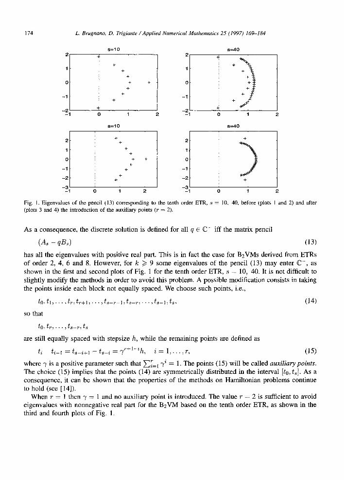
Fig. 1. Eigenvalues of the pencil (13) corresponding to the tenth order ETR, s = 10, 40, before (plots 1 and 2) and after (plots 3 and 4) the introduction of the auxiliary points (r = 2).

As a consequence, the discrete solution is defined for all q E C - iff the matrix pencil

(As - qBs) (13)

has all the eigenvalues with positive real part. This is in fact the case for B2VMs derived from ETRs of order 2, 4, 6 and 8. However, for k ~> 9 some eigenvalues of the pencil (13) may enter C - , as shown in the first and second plots of Fig. 1 for the tenth order ETR, s = 10, 40. It is not difficult to slightly modify the methods in order to avoid this problem. A possible modification consists in taking the points inside each block not equally spaced. We choose such points, i.e.,

to , t l , . . . , t r , t r + l , . • • , t s - - r - -1 , t s - - r , . • • , t s - - l , t s , (14)

SO that

to , t r , • • • , t s - r , t s

are still equally spaced with stepsize h, while the remaining points are defined as

t i - t i - l = t s - i + l - t s - i = T r + l - i h , i = l , . . . , r , (15)

where 7 is a positive parameter such that }--~i~l 7 ~ = 1. The points (15) will be called a u x i l i a r y p o i n t s .

The choice (15) implies that the points (14) are symmetrically distributed in the interval [to, ts]. As a consequence, it can be shown that the properties of the methods on Hamiltonian problems continue to hold (see [14]).

When r = 1 then 7 = 1 and no auxiliary point is introduced. The value r = 2 is sufficient to avoid eigenvalues with nonnegative real part for the B2VM based on the tenth order ETR, as shown in the third and fourth plots of Fig. 1.

L. Brugnano, D. Trigiante / Applied Numerical Mathematics 25 (1997) 169-184 175

The above choice of the points (14) is able to guarantee A-stability for B2VMs derived from ETRs, as stated by the next result.

Theorem 3.1. Let the method (11) be derived from ETRs and suppose that the corresponding pencil (13) has all the eigenvalues with positive real part. The method is then A-stable.

Proof. Suppose, in fact, to apply the method to the test equation

z' = oAz, Z(to) = 1, (16)

where o~ • R and i is the imaginary unit. Since the pencil (13) has all the eigenvalues with positive real part, from the maximum-modulus theorem, it follows that the thesis holds true iff Izj.sl <. 1, j = 1 , . . . , p , independently of c~ and of the stepsize h used. Let us prove the thesis for j = 1, since the result can be readily generalized by induction. For this purpose, let us denote

z = ~ + i ~ , ~,~ • R.

Consequently, Eq. (16) can be recast in the equivalent real form

(0 l) y ' = c~ 0 Y' y(to) = , y : . (17)

It is easily verified that problem (17) is Hamiltonian, with Hamiltonian function

yTy = ~2 + ~2 = izl 2.

For B2VMs based on ETRs, Theorem 2.1 applies, thus giving (N --= s)

Izsl2 T = = y oyo = Iz012 = l ,

for all values of a and for any stepsize h. []

Remark 3.1. The previous result can be generalized to B2VMs based on symmetric schemes, as defined in [10,14]. In particular, ETRs belong to this wider family of methods.

4. Parallel implementation

The purpose of this section is to present the approaches followed for deriving an efficient parallel implementation of ETRs in both cases of IVPs and BVPs. A detailed presentation would be too long to be contained in this paper, so we confine ourselves to sketch the main ideas (see [2,3,14,15]). In order to simplify the presentation, we consider a linear autonomous problem of size m,

y' = Ly + g(t), t • It0, T], V(to) = ~7, (18)

to describe the parallel algorithm. Supposing that the coarse mesh (10) is fixed, the use of a B2VM over the entire interval [to, T]

leads to the following lower block bidiagonal linear system:

M ( P ) y (p) : g(P), (19)


where

M(p) =

Vl

½ M2 , y(p) = " . ",. / J

Y2 , g(P) = h292 ,

yp \ hpgp /

the block vector yj (see (12)) contains the discrete approximation to the solution over the j th subinterval of the coarse mesh, and 9j is a block vector containing suitable combinations of the inhomogeneity in (18) at the points in the same subinterval. The block matrices Mj are defined as (see (6)-(7))

Mj = As ® Im - hjBs ® L, j = 1,.. . ,p.

Finally,

V j = [ O l v j ] , j = 2 , . . . , p ,

where O is the sm x (s - 1)m zero matrix and

vj = as @ Im - hjbs ® L, j = 1,.. .,p.

The parallel algorithm, working on p parallel processors, then consists in assigning the subproblem over the j th subinterval to the j th processor, j = 1 , . . . , p . This is done by considering the following factorization of the coefficient matrix:

(20) M(p) r)(p) r~(p)

where

D}p) M1 and D~ p) wl = . = L

Hereafter, for any integer r we set/~r = / ~ ® Ira, and for all allowed j, Wj = [O t wj], where wj is the solution of the linear system

M j w j = v j , j = l , . . . , p .

Of course, each block Mj, which represents the application of the method over the subinterval [~-j_ t, ~-j] of the coarse mesh, must be nonsingular. When L has no eigenvalues with positive real part, the previous Theorem 3.1 implies that each block Mj is nonsingular, whatever is the stepsize hj used.

The solution of Eq. (19) is then obtained by first solving the block diagonal system

D}P)x (p) = g(P), (21)

and then the block lower bidiagonal one

D~P) y (p) = x (p). (22)

For convenience, we partition the auxiliary vector x (p) as done for y(P),

x(p) T : . , W p ) , XO C ]l~ rn, X j E I~ srn.

L. Brugnano, D. Trigiante /Appl ied Numerical Mathematics 25 (1997) 169-184 177

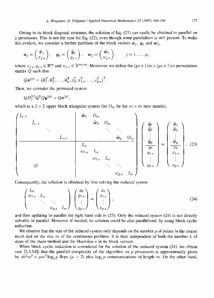
Owing to its block diagonal structure, the solution of Eq. (21) can easily be obtained in parallel on p processors• This is not the case for Eq. (22), even though some parallelism is still present• To make this evident, we consider a further partition of the block vectors x j, y j and wj ,

( ~ y ) ( ~ t j ) , w j = ( ~ j ) j = l , . . . , p , X j : Xj . s ' YJ : Yj .s Wj . s '

where Xy.s, Yj.s E ]R "~ and wj.~ E R "~×m. Moreover, we define the (ps + 1)m × (p8 + 1)m permutation matrix Q such that

z . ~ p ~ X O ~ 1.s~.. •~xp . s ) .

Then, we consider the permuted system

QD~p) QT Qy (p) = Qx (p),

which is a 2 × 2 upper block triangular system (let Om be the m × m zero matrix),

0

'm 1 Om

"~2

Wl .s

W2.s

~p O~

wps

Yp =

Yl .s

A

X2

A Xp

T (23)

Xl.s

\ Xp.s /

Consequently, the solution is obtained by first solving the reduced system

wls Im y l s (24)

" • • " • • "

Wp.s [rn Yp.s / Xp.s

and then updating in parallel the right hand side in (23)• Only the reduced system (24) is not directly solvable in parallel• However, if needed, its solution could be also parallelized, by using block cyclic reduction•

We observe that the size of the reduced system only depends on the number p of points in the coarse mesh and on the size m of the continuous problem. It is then independent of both the number k of steps of the main method and the blocksize s in its block version•

When block cyclic reduction is considered for the solution of the reduced system (24), we obtain (see [2,3,14]) that the parallel complexity of the algorithm on p processors is approximately given by skZm 3 + Itm 3 log 2 p flops (# = 2) plus log 2 p communications of length m. On the other hand,

178 L Brugnano, D. Trigiante / Applied Numerical Mathematics 25 (1997) 169-184

the sequential complexity for solving (19) amounts to approximately psk2m 3 flops. Consequently, the expected speed-up on p processors is given by

P Sp ~ 1 + (#logzp)/(sk2)" (25)

It is worth nothing that Sp rapidly approaches p, as k and s grow. Concerning the case of two-point boundary value problems, let us consider the following linear

problem,

y'(t) = Ly(t) + 9(t), Boy(to) + Bly (T) = ~7,

where/3o and B1 are m × m matrices and ~ c ~m. The discrete problem is still given by Eq. (19), which now assumes the following form, (io) ( /

Vl M1 Yl h~gl V2 M2 Y2 = h292 ,

"o. ". .

Vp mp p hpgp

where 0 is the m × ( s - 1)m zero vector. In this case, however, the factorization (20) cannot be considered for obtaining a parallel algorithm, because of stability reasons (the diagonal blocks My, in fact, are in general ill conditioned or even singular). Nevertheless, a different factorization can still be defined, originating a parallel algorithm whose speed-up is given by (25) with p = 20/3. We refer to the above quoted references for details.

5. Numerical tests

In this section we report some numerical tests carried out on both sequential and parallel computers. The comparison among different codes is a difficult task, which requires to fix significant evaluation parameters. For example, it is reasonable to compare methods having similar stability properties. Nevertheless, due to the complexity of the implementation strategies, the most significant evaluation parameter seems to be the execution time on the same computer. For this reason, we refrain from generic considerations on the advantages of ETRs. Instead, we prefer to report some comparisons with the code RADAU5 [17], whose reliability is well known.

The sequential tests concerning IVPs are obtained by using a code currently being developed by Iavernaro and Mazzia [18]. It performs quite well, even though it still requires to be fully optimized. We also report results on a couple of BVPs, obtained by using a Matlab prototype implementing a new mesh selection strategy, recently defined in [12]. For the tests on parallel computer, we have used a prototype of code which works for linear problems, both IVPs and BVPs. All the codes are based on BzVMs derived from ETRs.

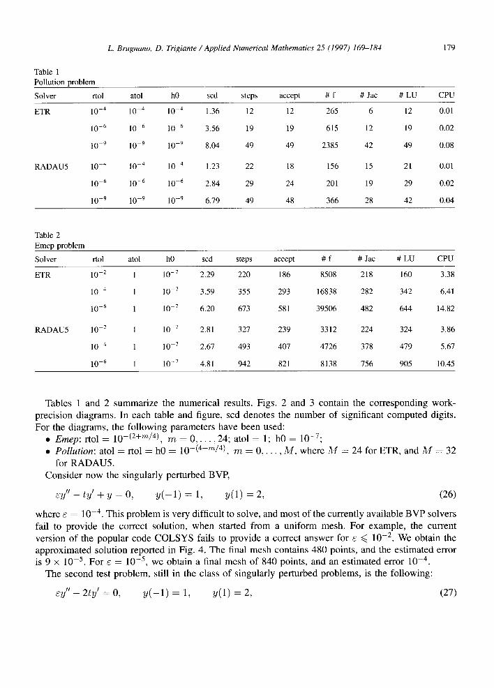
The test problems for the sequential code, which works on IVPs, are taken from the test set [19]. In particular, the Pollution problem (ODE of dimension 20) and the Emep problem (ODE of dimension 66) have been considered. The runs were performed on an Alpha workstation 200 4/233 using the Fortran 77 compiler with optimization f7 7 -0 4 -0 5. The code has been compared with RADAU5.

L. Brugnano, D. Trigiante /Applied Numerical Mathematics 25 (1997) 169-184 179

Table 1 Pollution problem

Solver rtol atol h0 scd steps accept # f # Jac # L U CPU

ETR

RADAU5

10 -4 10 4 10-4 1.36 12 12 265 6 12 0.01

10 -6 l0 -6 l0 6 3.56 19 19 615 12 19 0.02

10 - 9 10 9 10 - 9 8.04 49 49 2385 42 49 0.08

10 -4 10 -4 10 -4 1.23 22 18 156 15 21 0.01

10 -6 10 -6 10 -6 2.84 29 24 201 19 29 0.02

10 - 9 10 - 9 10 - 9 6.79 49 48 366 28 42 0.04

Table 2 Emep problem

Solver rtol atol h0 scd steps accept # f # Jac # LU CPU

ETR

RADAU5

10 2 1 10 -7 2.29 220 186 8508 218 160 3.38

10 4 1 10 -7 3.59 355 293 16838 282 342 6.41

10 - 6 1 10 -7 6.20 673 581 39506 482 644 14.82

10 -e 1 10 7 2.81 327 239 3312 224 324 3.86

10 4 1 10 7 2.67 493 407 4726 378 479 5.67

10 6 1 10 - 7 4.81 942 821 8138 756 905 10.45

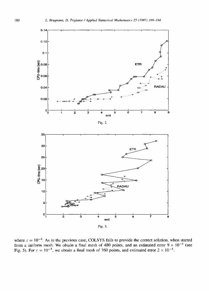
Tables 1 and 2 summarize the numerical results. Figs. 2 and 3 contain the corresponding work- precision diagrams. In each table and figure, scd denotes the number of significant computed digits. For the diagrams, the following parameters have been used:

• E m e p : rtol = 10 -(2+m/4), rrt z 0 , . . . ,24; atol = 1; h0 = 1 0 - 7 ;

• Pol lu t ion: atol = rtol = h0 = 10 -(4+m/4), zr~ z 0 , . . . , M , where M = 24 for ETR, and M = 32 for RADAU5.

Consider now the singularly perturbed BVP,

c y " - t y ' + y = 0, y ( - 1 ) = 1, y(1) = 2, (26)

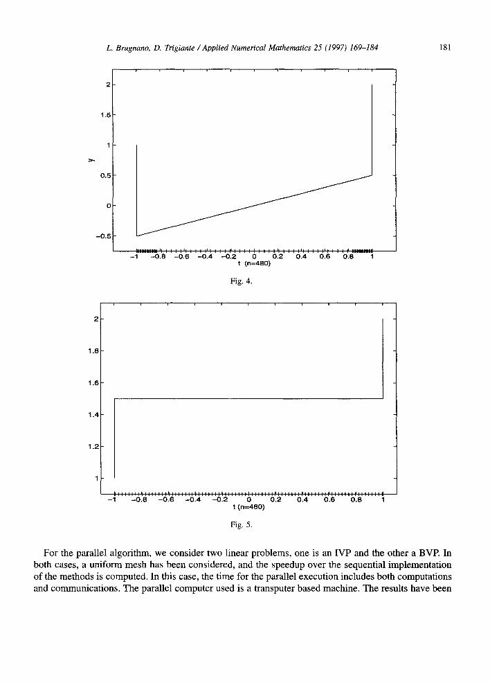
where e = 10 - 4 . This problem is very difficult to solve, and most of the currently available BVP solvers fail to provide the correct solution, when started from a uniform mesh. For example, the current version of the popular code COLSYS fails to provide a correct answer for e <~ 10 -2. We obtain the approximated solution reported in Fig. 4. The final mesh contains 480 points, and the estimated error is 9 x 10 -5. For c = 10 -5, we obtain a final mesh of 840 points, and an estimated error 10 -4.

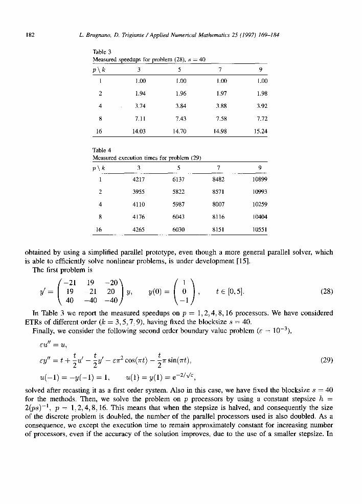
The second test problem, still in the class of singularly perturbed problems, is the following:

ey" - 2 t J = 0, y ( - 1 ) = 1, y(1) = 2, (27)

180 L. Brugnano, D. Trigiante /Applied Numerical Mathematics 25 (1997) 169-184

0.14 . . . . . . . .

0.12

0.1

A 0

,~ 0.08

E

0.06 0

0.04

0.02

O O

ETR 4 -

- F , ' " ÷

4 - . . . . . . - ~

~_~.."+ RADAU

+..._H_+.~.:.-+ +. . ~ + ...... + ........ ÷ ~. -""~

I f I I I I I

1 2 3 4 5 6 7 8 9 scd

Fig. 2.

35

30

25

"G" ~ 2 0

¢D

E

0 .

10 4-'.'. " . . ~

.~ . . . . . . "'.'.'.4-

+""4- ~ + Y

I I I I I

2 3 4 5 6 scd

Fig. 3.

I

7 8

where e = 10 -4. As in the previous case, COLSYS fails to provide the correct solution, when started from a uniform mesh. We obtain a final mesh of 480 points, and an estimated error 9 × 10 -5 (see Fig. 5). For e = 10 -5, we obtain a final mesh of 760 points, and estimated error 2 × 10 -5.

L. Brugnano, D. Tri giante /Applied Numerical Mathematics 25 (1997) 169-184 181

1.5

0.5

- 0 . 5

J J

I J

J J

J J

J J

J J

J

-1 -0 .8 - 0 . 6 -0 .4 -0 .2 0 0.2 0.4 0.6 0.8 1 t (n=480)

Fig. 4.

1.8

1.6

1.4

1.2

h . . . . . . . b . . . . . . . h . . . . . . . b . . . . . . . I . . . . . . . I . . . . . . . I . . . . . . . I . . . . . . . d . . . . . . . d . . . . . . . d

-1 - 0 . 8 - 0 . 6 - 0 . 4 - 0 . 2 0 0.2 0.4 0.6 0.8 1 t (n=480)

Fig. 5.

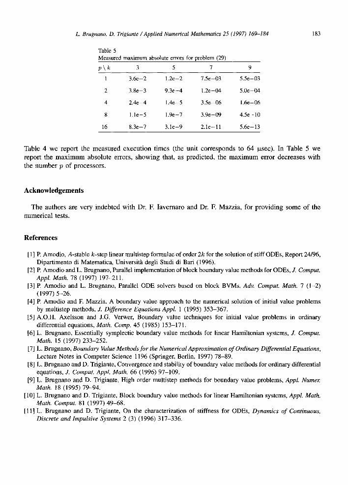
For the parallel algorithm, we consider two linear problems, one is an IVP and the other a BVE In both cases, a uniform mesh has been considered, and the speedup over the sequential implementation of the methods is computed. In this case, the time for the parallel execution includes both computations and communications. The parallel computer used is a transputer based machine. The results have been


Table 3 Measured speedups for problem (28), s = 40

p \ k 3 5 7 9

1 1.00 1.00 1.00 1.00

2 1.94 1.96 1.97 1.98

4 3.74 3.84 3.88 3.92

8 7.11 7.43 7.58 7.72

16 14.03 14.70 14.98 15.24

Table 4 Measured execution times for problem (29)

p\ I¢ 3 5 7 9

1 4217 6137 8482 10899

2 3955 5822 8571 10993

4 4110 5987 8007 10259

8 4176 6043 8116 10404

16 4265 6030 8151 10551

obtained by using a simplified parallel prototype, even though a more general parallel solver, which is able to efficiently solve nonlinear problems, is under development [15].

The first problem is

- 2 1 19 yt = 19 - 2 1

40 - 4 0

2o) (o) 20 y, y(0) = , t E [0, 5]. (28)

- 4 0 1

In Table 3 we report the measured speedups on p = 1 ,2 ,4 , 8, 16 processors. We have considered ETRs of different order (k = 3, 5, 7, 9), having fixed the blocksize s = 40.

Finally, we consider the following second order boundary value problem (e = 10-3),

~ U It = U,

t e y " = t + 2 u ' - 2 # ' - eTr 2 c o s ( T r t ) - 5zr sinQrt), (29)

u ( - 1 ) = - V ( - 1 ) = 1, u(1) = V(1) = e -2/v~,

solved after recasting it as a first order system. Also in this case, we have fixed the blocksize s = 40 for the methods. Then, we solve the problem on p processors by using a constant stepsize h = 2(ps) -1, p = 1, 2 ,4 , 8, 16. This means that when the stepsize is halved, and consequently the size of the discrete problem is doubled, the number of the parallel processors used is also doubled. As a consequence, we except the execution time to remain approximately constant for increasing number of processors, even if the accuracy of the solution improves, due to the use of a smaller stepsize. In

L. Brugnano, D. Trigiante / Applied Numerical Mathematics 25 (1997) 169-184

Table 5 Measured maximum absolute errors for problem (29)

p \ k 3 5 7 9

1 3.6e-2 1.2e-2 7.5e-03 5.5e-03

2 3.8e-3 9.3e-4 1.2e-04 5.0e-04

4 2.4e-4 1.4e-5 3.5e-06 1.6e-06

8 1. le-5 1.9e-7 3.9e-09 4.5e- 10

16 8.3e-7 3.1e-9 2.1e-11 5.6e-13

183

Table 4 we report the measured execution times (the unit corresponds to 64 p.sec). In Table 5 we report the maximum absolute errors, showing that, as predicted, the maximum error decreases with the number p of processors.

Acknowledgements

The authors are very indebted with Dr. E Iavernaro and Dr. F. Mazzia, for providing some of the numerical tests.

References

[1] R Amodio, A-stable k-step linear multistep formulae of order 2k for the solution of stiff ODEs, Report 24/96, Dipartimento di Matematica, Universit,5 degli Studi di Bari (1996).

[2] P. Amodio and L. Brugnano, Parallel implementation of block boundary value methods for ODEs, J. Comput. Appl. Math. 78 (1997) 197-211.

[3] P. Amodio and L. Brugnano, Parallel ODE solvers based on block BVMs, Adv. Comput. Math. 7 (1-2) (1997) 5-26.

[4] P. Amodio and E Mazzia, A boundary value approach to the numerical solution of initial value problems by multistep methods, J. Difference Equations Appl. 1 (1995) 353-367.

[5] A.O.H. Axelsson and J.G. Verwer, Boundary value techniques for initial value problems in ordinary differential equations, Math. Comp. 45 (1985) 153-171.

[6] L. Brugnano, Essentially symplectic boundary value methods for linear Hamiltonian systems, J. Comput. Math. 15 (1997) 233-252.

[7] L. Brugnano, Boundary Value Methods for the Numerical Approximation of Ordinary Differential Equations, Lecture Notes in Computer Science 1196 (Springer, Berlin, 1997) 78-89.

[8] L. Brugnano and D. Trigiante, Convergence and stability of boundary value methods for ordinary differential equations, J. Comput. Appl. Math. 66 (1996) 97-109.

[9] L. Brugnano and D. Trigiante, High order multistep methods for boundary value problems, Appl. Numer. Math. 18 (1995) 79-94.

[10] L. Brugnano and D. Trigiante, Block boundary value methods for linear Hamiltonian systems, Appl. Math. Math. Comput. 81 (1997)49-68.

[ 11 ] L. Brugnano and D. Trigiante, On the characterization of stiffness for ODEs, Dynamics of Continuous, Discrete and Impulsive Systems 2 (3) (1996) 317-336.


[12] L. Brugnano and D. Trigiante, A new mesh selection strategy for ODEs, Appl. Numer. Math. 24 (1997) 1-21.

[13] L. Brugnano and D. Trigiante, Boundary value methods: The third way between linear multistep and Runge-Kutta methods, Comput. Math. Appl. (to appear).

[14] L. Brugnano and D. Trigiante, Solving Differential Problems by Multistep Initial and Boundary Value Methods (Gordon & Breach, to appear).

[15] L. Brugnano and D. Trigiante, Parallel implementation of block boundary value methods on nonlinear problems: theoretical results, in preparation.

[16] J.R. Cash, Stable Recursions (Academic Press, London, 1979). [17] E. Hairer and G. Wanner, Solving Ordinary Differential Equations II, Springer Series in Computational

Mathematics 14 (Springer, Berlin, 1991). [18] E Iavernaro and F. Mazzia, The ETR code for stiff initial value problems, in preparation. [19] W.M. Lioen, J.J.B. de Swart and W.A. van der Veen, Test set for IVP solvers, CWI Report NM-R9615,

Amsterdam (1996). [20] I. Sgura, Approssimazione numerica di ODE con metodi BVM: propriet~i, applicazioni e confronti, Tesi di

Dottorato di Ricerca, Pisa (1996).

on the potentiality of sequential and parallel codes...

Documents