on the resilience of ant algorithms. experiment with
TRANSCRIPT

mathematics
Article
On the Resilience of Ant Algorithms. Experimentwith Adapted MMAS on TSP
Elena Nechita 1,*, Gloria Cerasela Crisan 1, Laszlo Barna Iantovics 2 and Yitong Huang 3
1 Department of Mathematics and Informatics, Vasile Alecsandri University of Bacău, 600115 Bacău, Romania;[email protected]
2 Department of Electrical Engineering and Information Technology, George Emil Palade University ofMedicine, Pharmacy, Science and Technology of Târgu Mures, 540139 Târgu Mures, Romania;[email protected]
3 Computer Science Department, Illinois Institute of Technology, Chicago, IL 60616, USA;[email protected]
* Correspondence: [email protected]
Received: 30 March 2020; Accepted: 27 April 2020; Published: 9 May 2020�����������������
Abstract: This paper focuses on the resilience of a nature-inspired class of algorithms. The issuesrelated to resilience fall under a very wide umbrella. The uncertainties that we face in the world requirethe need of resilient systems in all domains. Software resilience is certainly of critical importance,due to the presence of software applications which are embedded in numerous operational andstrategic systems. For Ant Colony Optimization (ACO), one of the most successful heuristic methodsinspired by the communication processes in entomology, performance and convergence issues havebeen intensively studied by the scientific community. Our approach addresses the resilience ofMAX–MIN Ant System (MMAS), one of the most efficient ACO algorithms, when studied in relationwith Traveling Salesman Problem (TSP). We introduce a set of parameters that allow the managementof real-life situations, such as imprecise or missing data and disturbances in the regular computingprocess. Several metrics are involved, and a statistical analysis is performed. The resilience of theadapted MMAS is analyzed and discussed. A broad outline on future research directions is given inconnection with new trends concerning the design of resilient systems.
Keywords: resilience; nature-inspired algorithm; Ant Colony Optimization; MAX–MIN Ant System;Traveling Salesman Problem
1. Introduction
In recent decades, the community of researchers from various domains has shown a growinginterest towards systems resilience. Of course, systems of any kind are expected to meet requirementsand maintain their operational characteristics as long as possible, while facing changing (sometimesunpredictable) conditions, environments and challenges. The concept of resilience has emergedfor complex, dynamic systems and can be generally defined as “the capacity of a system totolerate disturbances while retaining its structure and functions” [1]. The list of domains wheresystems resilience is important is long, and specific definitions have been provided: engineering [1],economics [2,3], environment [4,5], ecology [6,7], psychology and neurobiology [8–10], sociology [11].In computer science, resilience has been defined mainly for networks [12–15] and large-scale distributedsystems [16,17], security [18] and soft infrastructure systems [19]. The term resilience is derived fromthe Latin “resilire”, with the meaning “springing back” or “jumping back up”, which sends us to theviews of resilience considering the recovery of a system after facing adverse situations.
Given the wide interest and importance of the concept, not only for researchers but for policymakerstoo, numerous and sometimes diverging interpretations and perceptions have been proposed for
Mathematics 2020, 8, 752; doi:10.3390/math8050752 www.mdpi.com/journal/mathematics

Mathematics 2020, 8, 752 2 of 20
resilience. Several studies proposed conceptual and theoretical models for resilience, such as Cutter etal. [20], Jordan and Javernick-Will [21] for societal resilience, Scott [22], MacAskill and Guthrie [23] fordisaster risk management or Chien et al. [24] for high-performance computing systems. A methodologyto draw together resilience concepts from multiple disciplines can be found in Wright et al. [25].
Considerations on resilience, as it was defined and approached by researchers in various domainsof human activity, are given in Section 2, which also bridges this concept with that of algorithmicperformance. Section 3 overviews some basic ideas and characteristics of the ant algorithms anddescribes the tools: Traveling Salesman Problem (TSP) as test problem and MMAS to be adapted tothe research goals. Section 4 points to the experimental settings. Section 5 presents the experimentaloutputs and their statistical analysis, while Section 6 concludes on the research results and gives somelines for further investigations.
2. The Concept of Resilience and Some of Its Instances
This section presents the concept of resilience as it evolved over the ages and across areas ofhuman activity and research, with the intent to underline its main characteristics and emphasize bothits essence and its multiple facets.
For physical and social systems, resilience is defined in Bruneau and Reinhorn [26] as consistingof the following properties: robustness (the ability of elements to withstand a given level of stress ordemand without suffering degradation or loss function), redundancy (the extent to which the system’selements are substitutable), resourcefulness (the capacity to identify problems, establish priorities andmobilize resources when disruption conditions manifest), and rapidity (the capacity to meet prioritiesand achieve goals in a timely manner in order to recover functionality and avoid future disruption).Defining the concepts of vulnerability and resilience, Proag [27] differentiates between two broadforms of the last one: hard resilience—the direct strength of a structure when placed under pressure,and soft resilience—the ability of systems to absorb and recover from the impact of disruptive eventswithout fundamental changes in function or structure.
The need for designing systems that allow for their evolvability has been recognized [28], sincethe majority of changes that a system is going to cope with are not foreseeable at the moment of itsdesign. Technology refreshment programs have been proposed [29] to enhance systems capability forfacing external sources of change.
Computer scientists have used the term “resilient” since 1976 and use it more and more often,sometimes as a synonym of fault-tolerant [30]. Avizienis et al. [31] define resilience as “the persistenceof service delivery that can justifiably be trusted, when facing changes” or “the persistence of avoidanceof failures that are unacceptably frequent or severe, when facing changes”. Resilient software systemsare needed in applications executed on distributed platforms (very often, with a dynamically changingtopology), satisfying real-time requirements, interacting with real-world and managed externally by anauthority. Approaching software resilience implies to model the functionality that the system provides,the way the system can provide that functionality and the deployment of constraints. Axelrod [32] notesthe definition given in Marcus and Stern [33] for a resilient system: “one that can take a hit to a criticalcomponent and recover and come back for more in a known, bounded, and generally acceptable periodof time” and presents the factors that may diminish software resiliency: complexity, interdependencyand interconnectivity, globalization, hybridization, rapid change and reuse in different contexts.
In Chandra [34], an extensive study regarding the synergy between biology and systems resilienceis given. The thesis focuses on extracting principles and heuristics useful for designing resilientengineering systems, based on the resilience seen in nature. Resilience attributes (adaptability,redundancy, scalability, self-organization, interoperability, dynamic learning) are identified in immunesystems, colonies of social insects and ecosystems, and a domain-independent qualitative model ofresilience is developed.
When talking about resilience, it is important to measure it. Enhancing the resilience of a systeminvolves the understanding of the relationships that exist between the various components of that

Mathematics 2020, 8, 752 3 of 20
system. Although models for systems resilience can be useful, these should be interpreted on specificcontext and purpose [35] and it is important to be able to quantify the resilience of systems.
Measuring resilience naturally depends on the system being studied. While qualitative assessmentreveals how bad a system can be disturbed, quantitative measures give estimates of performance [36].Some general considerations on metrics for resilience are given in Ford et al. [18].
For the purposes of our work, which approaches TSP with a nature-inspired type of algorithm,we have used several metrics, further described in Section 4.3.
3. Adaptation of an Ant Algorithm to Allow Disturbances Simulation
During the last century, TSP was one of the most studied NP-hard problems in CombinatorialOptimization and Operations Research, mostly due to its applications in industry, transportation andlogistics. The ant colony metaphor was easily adapted to TSP. Sections 3.1–3.4 present the foundationsof the ant algorithmic approach, TSP as test problem and the particular Ant algorithm adapted fortackling real-world issues of TSP.
3.1. An Efficient Nature-Inspired Class of Algorithms
An ant colony is an example of a highly distributed natural, cooperative multiagent system. It iscomprised of hundreds (or thousands) of completely autonomous simple agents (the ants) and is robustwith respect to loss of individual agents and to changes in the environment [37]. The performanceof the activities of the colony can be seen as highly effective [38] and are, in some cases, optimalor near-optimal.
In a colony, the scouts are the ants exploring the territory around the nest in search for food. At thebeginning, a scout wanders and finds a food source only by chance. As a result, the route the scoutant follows from the nest to the food source displays a random pattern. Conversely, the route backis straight-lined and impregnated with pheromones, which are a very elaborated form of chemicalcommunication [39]. The scout alerts its worker mates, who follow the pheromone trail to the foodsource. The number of ants using the trail is proportional to the available amount of food and, as longas the food source is not exhausted, the ants will reinforce the path while carrying their load back to thenest. This behavior determines higher and higher concentrations of pheromone on the shorter paths, asmore and more ants are using them. On longer paths, the pheromone concentration decays over time.
Based on this ant foraging model, Dorigo et al. [40,41] have founded a new paradigm ofevolutionary computation that has come to be known as Ant Colony Optimization (ACO) [42]. ACO isperhaps the most successful application inspired by ants—and perhaps by any insect society. Thereare three ideas from natural ant behavior that have been transferred to the artificial ant colony: thepreference for paths with high pheromone level, the higher rate of growth of pheromone on shorterpaths and the trail mediated communication among ants.
Since its development, researchers have applied ACO to a significant number of combinatorialoptimization problems including the Traveling Salesman Problem (TSP), the Vehicle Routing Problem,graph coloring, allocation problems, swarm robotics, routing in telecommunication networks, constraintsatisfaction and many other related issues.
3.2. TSP as Test Problem
TSP [43–45] was the first combinatorial optimization problem successfully solved with ACO [41].We chose the Euclidean TSP as a support problem for the experiments on the resilience of ant algorithmsimplementations mostly due to its numerous real-life applications, most of which involve uncertainty.This characteristic is highly adequate for the aim of our study, namely, to analyze the ant algorithmscapacity to “turn back” towards good solutions, even after significant interventions in the normal ACOexecution process.
Given a map with n sites and their pairwise distances, TSP requires finding one shortest cyclic tourthrough all the sites or, more formally, the least cost Hamiltonian cycle in a weighted graph. Formally,

Mathematics 2020, 8, 752 4 of 20
let G = (N, A), with N the set of nodes (locations) and A the set of arcs fully connecting the nodes.Each arc (i, j) is assigned the positive value d(i, j) which is the distance between locations i and j. TSP isthe problem of finding the shortest closed tour visiting the n = |N| nodes of G exactly once.
TSP is a NP-hard problem [46]. However, polynomial time exact algorithms are available inparticular cases [47]. Relaxation methods [48,49] have been used to develop Concorde [50], the best TSPexact solver at present. However, there are practical situations that could efficiently use results providedwith approximate methods for TSP models [44,51–54]. Heuristic and metaheuristic approaches forTSP have also been intensively studied: local search [55–57], Lin–Kernigan [58], chained Lin–Kerniganmethods [59], simulated annealing [60,61], genetic algorithms [62], and ant colony optimization(ACO) [42,63].
3.3. Implementations of Ant Algorithms for TSP
The software package ACOTSP [64], freely available for both researchers and practitioners,includes implementations of ACO Algorithms for the symmetric TSP: Ant System, Elitist Ant System,MAX–MIN Ant System, Rank-based Ant System, Best–worst Ant System, and Ant Colony System.The performance of these implementations depends on instance dimension, parameter variationstrategies, and particular improvements that may be operated upon (such as ants’ specialization [65],human intervention in the ant loop [66], pheromone correction methods [67]) but is generally perceivedby the scientific community as reasonably high. What makes these implementations very “usable” istheir capacity to return as high-quality solutions as possible, independently of the allowed computationtime [68,69].
Ant System (AS) was the first ACO algorithm, proposed by Dorigo et al. in 1991 [70–72].The algorithm of TSP solving with AS assumes a colony of m artificial ants that operate on the graph Gand a pheromone matrix τ =
{τi j
}for the construction of the solutions. At the beginning, τi j are set
to the same initial, positive value. The m ants are randomly deployed in the nodes of G. Within tmax
iterations, the following repeat.Each ant constructs a complete tour using Equation (1) below. If t is the index of the current
iteration, an ant k currently at node i chooses the node j to move to (from the set Jk(i) of the nodes notvisited yet) by applying the following probabilistic transition rule:
pki j(t) =
[τi j(t)]
α×[ηi j]
β∑lεJk(i)
[τil(t)]α×[ηil]
β , i f jεJk(i)
0, otherwise(1)
where ηi j = 1/d(i, j) stands for the heuristic information called “visibility” of arc (i, j), while τi j(t)represents the “desirability” that the arc (i, j) belongs to the tour of the ant k. This desirability reflects theexperience acquired by ants during the problem-solving and models a learning process. Parameters αand β set the balance between the influence of the pheromone level and that of the heuristic information.Pheromone update is applied according to Equation (2) for all ants k and all arcs(i, j):
τki j(t + 1) = (1− ρ)·τk
i j(t) + ∆τki j(t) (2)
where ρ ∈ (0, 1] represents the proportion of the old pheromone quantity that is carried over to the nextiteration of the algorithm and the added quantity of pheromone as defined in Equation (3), with Tk(t)the tour built by ant k and Lk(t) its length:
∆τki j(t) =
{1/Lk(t), i f (i, j) ∈ Tk(t)
0, otherwise(3)
For our experimental study concerning the resilience of the ant algorithms, we have chosen theMAX–MIN Ant System (MMAS) proposed by Stützle and Hoos [73] to be modified according to the

Mathematics 2020, 8, 752 5 of 20
purpose of our research. Although the focus is on resilience and not on performance, it is important tonote that MMAS was designed as an algorithmic variant to achieve better performance than the antsystem, from which MMAS originates.
MMAS is the same as AS except that the pheromone trails are updated offline: only the arcs whichwere used by the best ant in the current iteration receive additional quantities of pheromones. Also,the pheromone trail values are placed in an interval [τmin, τmax] and the trails are initialized to theirmaximum value τmax.
Moreover, MMAS calls the 3-opt local search procedure [58] at the end of the tour completion forevery ant, thus being a hybrid method, which integrates both constructive and heuristic local-search.
3.4. New Parameters for MMAS
Let MMAS(epoch, p_nod_ch, p_inten, ampl) be the MAX–MIN Ant System enriched with a set ofparameters, which are described below. The role of the parameters resides in introducing variousdisturbances in the algorithmic loop which determines the solution construction.
The idea is to alter the pheromone matrix periodically. This process allow us to simulatefeatures such as uncertainty and dynamicity in the TSP instances to be approached with MMAS(epoch,p_nod_ch, p_inten, ampl). These features reside in numerous real-world problems that are modelledwith TSP, which justifies our approach. It assumes that the number of iterations when the systemworks without intervention defines the parameter epoch. At the beginning of MMAS(epoch, p_nod_ch,p_inten, ampl), the algorithm works as presented in Section 3.3. At the end of the first perioddefined by epoch (after a number of iterations equal to epoch), the values in the pheromone matrix arechanged non-deterministically: the degree of perturbation is introduced by means of the parametersp_nod_ch—the percentage of the nodes to suffer modifications, and p_inten—the percentage of arcsincident to the chosen nodes, arcs whose pheromone load are modified. The parameter ampl givesthe amplitude of the modification, setting an interval of length 2∗ampl∗old_value, centred in the oldpheromone value. The new pheromone value is randomly generated within this interval. The processrepeats all along the algorithmic loop of MMAS. The above parameters’ identifiers head the datacolumns in the files available at [74].
This design of MMAS was also used by Crisan et al. in [75] in order to perform an ant-basedsystem analysis on TSP under real-world settings, when comparing it with other hybrid optimizationtechniques. The feature introduced by these new parameters is the uncertainty that manifests in the realworld. This alteration of the pheromones may simulate missing or imprecise data, which frequentlyhappens in real-world systems that include TSP solvers.
4. Experimental Settings
Our experiment concerning the ant algorithms resilience was performed with the modifiedMMAS(epoch, p_nod_ch, p_inten, ampl) and three TSP instances. Specific details regarding instances,software, values for its parameters and organization of the output data are given below.
4.1. TSP Test InstancesThe instances chosen for tests in our experiment are from TSPLIB [76,77], the well-known library
of sample instances for combinatorial optimization problems. The problem names (which also includethe number of nodes of the corresponding graph) are d2103, fl3795 and rl1889. For all three, the2-dimensional Euclidean distances between nodes are rounded up to the next integer. The optimumtour lengths are known to be 80,450, 28,722 and 316,536, respectively.
d2103 is one of the instances proposed by Reinelt [76], coming from the practical problem ofdrilling holes in printed circuit boards. The drilling problem can be approached as a sequence of TSPinstances, one for each hole diameter [78]. fl3795 is another drilling instance, with a high degree ofdifficulty [79] given by the placement of the nodes in very particular clusters. The last instance, rl1889,is one of the examples drawn by Reinelt [76] from geographic problems featuring locations of citieson maps.

Mathematics 2020, 8, 752 6 of 20
4.2. Parameters Values and Ant ImplementationThe Ant implementation that we propose is synthetically described by the following algorithmic
scheme. The skeleton is according to [73], and the new parameters epoch, p_nod_ch, p_inten, amplare introduced.
procedure MMAS(epoch, p_nod_ch, p_inten, ampl)set parameters m, α, β, ρset the maximum pheromone trail τmax to an estimate/* the maximum possible pheromone trail is asymptotically bound */initialize pheromone trails to τmax
set epoch, p_nod_ch, p_inten, amplset previous_best and global_best to an initial solution /* e.g., found with Nearest-Neighbor heuristic */no_epochs = 0, better_sol = 0, epoch_previous_best = 0iteration = 0while (termination condition not met) do
iteration = iteration + 1ConstructSolutions/* each of the m ants builds its solution*/ApplyLocalSearch/* 3-opt local search procedure is called */set current_best to the best solution, delivered by best_antif current_best < global_best then
global_best = current_bestset global_time_best to the duration (seconds) required by best_ant to deliver its touriteration_best= iterationendifepoch_current_best = no_epochsUpdatePheromoneTrails/* only the arcs used by best_ant are updated *//* according to (2), (3) and the rules of pheromone update in MMAS */if iteration = epoch then
no_epochs = no_epochs + 1/* a new epoch starts */N1 = the set of
⌊p_nod_ch·|N|
⌋nodes randomly chosen from N
A1 = ∅for every node in N1 do
A1 = A1 ∪ {⌊p_inten·(no of arcs incident to the node)c arcs, randomly chosen}
end for/* alter the pheromone matrix */for every arc in A1 do
alter the pheromone load τ1 on the arc/* the new value is randomly chosen in [τ1 − τ1·ampl, τ1 + τ1·ampl] */
end forif (current_best < previous_best) and (epoch_current_best > epoch_previous_best) then
better_sol = better_sol + 1/* a better approximation was found, although the pheromone matrix was altered */
end ifend if
end whilerecovery_speed = better_sol/no_epochsreturn current_best, better_sol, global_time_best, iteration_best, no_epochs, recovery_speed
end
The original parameters used for MMAS(epoch, p_nod_ch, p_inten, ampl) in our experiments are:number of ants m = 25; α = 1; β = 2; ρ = 0.2.

Mathematics 2020, 8, 752 7 of 20
The values for the new parameters are as follows: epoch ∈ {20, 40, 60}; p_nod_ch ∈ {20, 40, 100};p_inten ∈ {50, 100}, ampl ∈ {0, 10, 20, 30, 40}.
For each of the three instances, all the 3·3·2·5 = 90 variants of MMAS, generated by the possiblecombinations of the parameter values, were executed. For each variant, ten trials have been performedin order to report a line in the result files, following the guidelines proposed by Birattari et al. [80].One core (of a dual-core processor at 2.5GHz frequency and 250 GB RAM) was assigned only for theexecution of MMAS software.
4.3. Recorded Data
For every TSP instance, the following execution outputs and statistics were recorded. These dataare stored in a file with the same identifier as the name of the instance, available for download at [74].
• better_solutions: number of times when the application manages to find a better approximationof the optimum tour, although the information stored on arcs (the pheromone quantities) wasdisturbed (averaged over ten trials).
• number of epochs: how many times during the execution the information on the arcs was disturbed(on average, in ten trials). During an epoch, the pheromones evolve according to Equations (2)and (3).
• average-best: this is the main metric based on which we study the algorithm resilience. It representsthe approximation of the TSP instance solution, as delivered by the modified ant algorithm MMAS(also averaged over ten trials).
• recovery speed: is the ratio between better_solutions and number of epochs. It gives a measure of therecovering capacity, showing how many times (on average, in ten trials) average-best improvesduring an epoch.
• average-iterations: is the average of the ten iteration numbers that found the best solution.• stddev-best: standard deviation for the ten best solutions delivered by the ten trials.• stddev-iterations: standard deviation for the ten iterations when the best solution was found.• best try: the best solution in ten trials.• worst try: the worst solution in ten trials.• avg. time-best: average of the times for finding the best solution in ten trials.• stddev.time best: standard deviation for the time durations needed to find the best solution, for the
ten trials.• distance-to-optimum: is the difference between the (average) solution found by the ant algorithm
(average-best) and the optimum solution.• relative-error: distance-to-optimum/optimum tour length ∗ 100.
Using the instance d2013 and the following values for the new parameters: epoch = 20, p_nod_ch = 20,p_inten = 50, ampl = 10 (which corresponds to line 22 in the data file d2013), the adapted MMAS worksas described below.
In a trial of MMAS(20, 20, 50, 10), after every 20 iterations, for b20/100·2103c = 420 nodes randomlychosen, the pheromone load is modified for half of the arcs (also randomly chosen) of the selectednodes. The number of arcs in this situation is 420·b50/100·2102c= 441,420. For every arc, the newpheromone value is randomly chosen in an interval of length 2·(10/100)·v, centred in v, which is the oldpheromone value. Under these settings, on average in 10 trials, we obtained the following outcome:
• number of epochs = 516. We obtained 516 series of 20 iterations and, starting with the second one,the pheromone alteration takes place as described above.
• better_solutions = 246, that is, although the pheromones are altered at every 20 iterations, thealgorithm improves the solution, getting closer to the optimum, 246 times.
• average-best = 80,555.5. This last approximation delivered by the algorithm is only at105.5 = distance-to-optimum (units) far from the known optimum, which is 80,450. We notice

Mathematics 2020, 8, 752 8 of 20
that 105.5 represents 0.13% (= the value of the relative-error) from the optimum. The algorithmsucceeded to provide a solution that is only 0.13% worse than the optimum, which is a very goodoutcome, given the repeated intervention into the solution construction mechanism. In terms ofresilience, we can assess that this is high for MMAS(20, 20, 50, 10).
• stddev-best = 54.64. The solutions delivered by the algorithm are spread around the average-best =
80,555.5 with a standard deviation of 54.64. The best solution among the ten collected in ten trialsis best try = 80,476 and the worst is worst try = 80,638.
• average-iterations = 633.5, that is, the average of the iteration numbers when the ten best solutionswere delivered. The standard deviation of these ten values is stddev-iterations = 249.93, quite abig value, showing that the best solution can be found early in the iterative process, or after asignificant number of iterations.
• avg. time-best = 36.81 s. This is the average value of the execution durations (measured in seconds)of the 10 trials. Given the computer system configuration that the experiment was processedon, the result is very good. The standard deviation for the execution times of the ten trials isstddev.time best = 13.
Finally, recovery speed = 0.4767 for this example. The value shows that, for instance d2103,MMAS(20, 20, 50, 10) improved the solution, on average, 0.4767 times per epoch.
5. Results and Statistical Analysis
5.1. Metrics for TSP Resilience Assessment with Adapted MMASAccording to Jackson [81], “System resilience is the ability of [...] systems to mitigate the severity
and likelihood of failures and loses, to adapt to changing conditions, and to respond appropriatelyafter the fact”.
Researchers in systems resilience point that resilience is not a 1-dimensional quantity [18].Moreover, a shift from robustness-centered design to principles of more flexible and adaptive designhas been noticed [33]. This approach includes the following ideas: composing the measures of differentaspects in order to reason about resilience; the metrics should be particular for a specific perturbation;the metrics should be dependent on the system boundaries; the customer requirements drive themetrics for resilience; take into consideration other aspects except for the system output. There is nouniversal way to combine the particular metrics into a global one, but the assessment process is specificto the synergy of all considered aspects.
When transferring the above considerations to the transportation field, resilience could be seenas the ability of transportation systems to react to unexpected disturbance. This can be seen at theindividual level, when transportation needs are satisfied for each customer, as well as at the communitylevel—such as in emergency state or special events, when this perspective comes first. Transportationsystems diversity (which includes multiple modes, routes, and system components) and criticalinformation related to collection and distribution are key elements for resilience [82]. Both thesefeatures can be modelled in ant algorithms [83].
In line with these considerations, when assigning the resilience of MMAS(epoch, p_nod_ch, p_inten,ampl) we chose to consider two kind of metrics:
• Time-performance metrics: better_solutions, number of epochs, average-iterations, stddev-iterations,avg. time-best, stdev.time best and recovery speed. All these data give us a feedback on how fast thealtered applications work.
• Path-performance metrics: average-best (which is the objective function) and stddev-best, best tryand worst try, three measures indicating how good the altered applications still perform.
Sections 5.2–5.4 present both a brief descriptive analysis (which can be used for a qualitativeassessment of the MMAS applications resilience) and a statistical one, based on the results of theexperiment, for each of the three TSP instances. The files presenting extensive statistical analysis areavailable at [74].

Mathematics 2020, 8, 752 9 of 20
For the descriptive analysis, only a part of the data from the files d2103, fl3795 and rl1889 wasextracted in Tables 1, 4 and 7, respectively. The tables present the results obtained for the metricsrecovery speed and average-best, reported for the highest value of ampl: 40%. That is, ifω is a pheromonevalue on a selected arc (according to p_nod_ch and p_inten) then the altered pheromone value randomlyfalls within the interval [0.6 ·ω, 1.40 ·ω]. These 18 variants of MMAS (of all 90) are those simulating themost substantial disturbances in the ACO constructive process of the approximate solution. Moreover,each table includes the lines for which the smallest and the highest values for the relative-error havebeen registered in all the 90 MMAS variants. For example, in Table 1, these correspond to executionswith ampl = 0 (which is the original MMAS, with no altered pheromones).
Table 1. Parameters and metrics for d2103, with ampl = 40.
Line p_nod_ch p_inten epoch recovery speed average-best relative-error
1 20 50 20 0.4487 80,595.2 0.182 20 50 40 1.1479 80,554.3 0.133 20 50 60 1.0877 80,546.1 0.124 20 100 20 0.5082 80,521.6 0.091
5 20 100 20 0.7103 80,593.8 0.186 20 100 40 0.8844 80,602.9 0.197 20 100 60 1.0838 80,596.2 0.188 40 50 20 0.4192 80,606.0 0.199 40 50 40 0.9000 80,590.1 0.17
10 40 50 60 1.0904 80,546.4 0.1211 40 100 20 0.6965 80,616.7 0.2112 40 100 40 0.8670 81,092.4 0.802
13 40 100 40 0.9945 80,564.2 0.1414 40 100 60 1.3642 80,529.4 0.1015 100 50 20 0.5019 80,537.9 0.1116 100 50 40 0.8445 80,587.0 0.1717 100 50 60 1.2384 80,557.8 0.1318 100 100 20 0.4173 80,583.8 0.1719 100 100 40 1.1618 80,647.5 0.2520 100 100 60 1.2051 80,561.8 0.14
1,2 Values for ampl=0.
For the statistical analysis, two directions are set. With epoch, p_nod_ch, p_inten and ampl as factors,the following are studied:
• The way the time-performance metrics depend on the factors and how these are inter-correlated.• The way the path-performance metrics depend on the factors and how these are inter-correlated.
The material displaying the results of the two approaches is quite extensive, and thus we presentin Tables 2, 3 (for d2103), 5, 6 (for fl3795), and 8, 9 (for rl1889), the regression models for the metricsaverage-best and recovery speed only. The factors for the non-zero values of the categorical variable ampl(the amplitude of the pheromone alteration) are ampl10%, ampl20%, ampl30%, and ampl40%.
The statistical analysis was performed with the free software environment for statistical computingand graphics R, version 3.4.4.
5.2. Discussion on Behaviour of Adapted MMAS with TSP Instance d2103The length of the optimum solution for the TSP instance d2103 is 80,450. As data in Table 1 display
in all lines except no. 4 and no. 12, the relative error for the 18 variants of MMAS with ampl = 40 isplaced in the interval [0.1, 0.25], corresponding to an absolute error (distance-to-optimum in the filed2013) in the interval [82.1, 197.5]. We note that the minimum but also the maximum relative-errorvalues (in lines 4 and 12) correspond to MMAS with ampl = 0.
For the original MMAS, recovery speed ∈[0.4934, 1.6154] (see file d2013), while for the applicationscorresponding to data in Table 1 (with ampl = 40), recovery speed ∈ [0.4173, 1.3642] and only three valuesare smaller than the minimum recovery speed for MMAS with ampl = 0. These findings show that
Mathematics 2020, 8, 752 10 of 20
MMAS(*,*,*, 40) continue to behave normally, in the sense of building efficient solutions for the instanceunder consideration, successfully recovering after pheromone alterations.
The tableau depicted by the metrics average-best and recovery speed allows us to qualitatively assessthe resilience of the adapted MMAS applications (according to the qualitative model in [34]) as High.
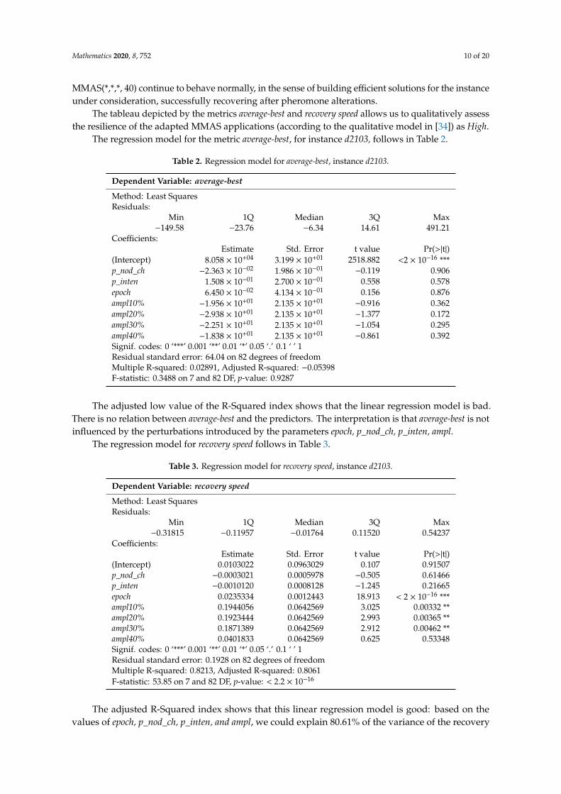
The regression model for the metric average-best, for instance d2103, follows in Table 2.
Table 2. Regression model for average-best, instance d2103.
Dependent Variable: average-best
Method: Least SquaresResiduals:
Min 1Q Median 3Q Max−149.58 −23.76 −6.34 14.61 491.21
Coefficients:Estimate Std. Error t value Pr(>|t|)
(Intercept) 8.058 × 10+04 3.199 × 10+01 2518.882 <2 × 10⁻¹⁶ ***p_nod_ch −2.363 × 10−02 1.986 × 10−01 −0.119 0.906p_inten 1.508 × 10−01 2.700 × 10−01 0.558 0.578epoch 6.450 × 10−02 4.134 × 10−01 0.156 0.876ampl10% −1.956 × 10+01 2.135 × 10+01 −0.916 0.362ampl20% −2.938 × 10+01 2.135 × 10+01 −1.377 0.172ampl30% −2.251 × 10+01 2.135 × 10+01 −1.054 0.295ampl40% −1.838 × 10+01 2.135 × 10+01 −0.861 0.392Signif. codes: 0 ‘***’ 0.001 ‘**’ 0.01 ‘*’ 0.05 ‘.’ 0.1 ‘ ’ 1Residual standard error: 64.04 on 82 degrees of freedomMultiple R-squared: 0.02891, Adjusted R-squared: −0.05398F-statistic: 0.3488 on 7 and 82 DF, p-value: 0.9287
The adjusted low value of the R-Squared index shows that the linear regression model is bad.There is no relation between average-best and the predictors. The interpretation is that average-best is notinfluenced by the perturbations introduced by the parameters epoch, p_nod_ch, p_inten, ampl.
The regression model for recovery speed follows in Table 3.
Table 3. Regression model for recovery speed, instance d2103.
Dependent Variable: recovery speed
Method: Least SquaresResiduals:
Min 1Q Median 3Q Max−0.31815 −0.11957 −0.01764 0.11520 0.54237
Coefficients:Estimate Std. Error t value Pr(>|t|)
(Intercept) 0.0103022 0.0963029 0.107 0.91507p_nod_ch −0.0003021 0.0005978 −0.505 0.61466p_inten −0.0010120 0.0008128 −1.245 0.21665epoch 0.0235334 0.0012443 18.913 < 2 × 10⁻¹⁶ ***ampl10% 0.1944056 0.0642569 3.025 0.00332 **ampl20% 0.1923444 0.0642569 2.993 0.00365 **ampl30% 0.1871389 0.0642569 2.912 0.00462 **ampl40% 0.0401833 0.0642569 0.625 0.53348Signif. codes: 0 ‘***’ 0.001 ‘**’ 0.01 ‘*’ 0.05 ‘.’ 0.1 ‘ ’ 1Residual standard error: 0.1928 on 82 degrees of freedomMultiple R-squared: 0.8213, Adjusted R-squared: 0.8061F-statistic: 53.85 on 7 and 82 DF, p-value: < 2.2 × 10⁻¹⁶
The adjusted R-Squared index shows that this linear regression model is good: based on thevalues of epoch, p_nod_ch, p_inten, and ampl, we could explain 80.61% of the variance of the recovery

Mathematics 2020, 8, 752 11 of 20
speed. The parameters p_nod_ch and p_inten are negatively correlated with recovery speed, whileepoch and ampl are positively correlated to it. The p values show that the factors epoch and ampl arestatistically significant in the model. Therefore, the recovery speed is influenced by the values of epochand ampl.
In Figure 1, the correlogram between the other time-performance metrics is displayed. Positivecorrelations are displayed in blue and negative correlations in red. Colour intensity and the size of thecircles are proportional to the correlation coefficients. In the right side of the correlogram, the legendcolour shows the correlation coefficients and the corresponding colours.
Mathematics 2020, 8, x FOR PEER REVIEW 11 of 21
Coefficients: Estimate Std. Error t value Pr(>|t|) (Intercept) 0.0103022 0.0963029 0.107 0.91507 p_nod_ch −0.0003021 0.0005978 −0.505 0.61466 p_inten −0.0010120 0.0008128 −1.245 0.21665 epoch 0.0235334 0.0012443 18.913 < 2 × 10⁻¹⁶*** ampl10% 0.1944056 0.0642569 3.025 0.00332 ** ampl20% 0.1923444 0.0642569 2.993 0.00365 ** ampl30% 0.1871389 0.0642569 2.912 0.00462 ** ampl40% 0.0401833 0.0642569 0.625 0.53348 Signif. codes: 0 '***' 0.001 '**' 0.01 '*' 0.05 '.' 0.1 ' ' 1 Residual standard error: 0.1928 on 82 degrees of freedom Multiple R-squared: 0.8213, Adjusted R-squared: 0.8061 F-statistic: 53.85 on 7 and 82 DF, p-value: < 2.2 × 10⁻¹⁶
The adjusted R-Squared index shows that this linear regression model is good: based on the values of epoch, p_nod_ch, p_inten, and ampl, we could explain 80.61% of the variance of the recovery speed. The parameters p_nod_ch and p_inten are negatively correlated with recovery speed, while epoch and ampl are positively correlated to it. The p values show that the factors epoch and ampl are statistically significant in the model. Therefore, the recovery speed is influenced by the values of epoch and ampl.
In Figure 1, the correlogram between the other time-performance metrics is displayed. Positive correlations are displayed in blue and negative correlations in red. Colour intensity and the size of the circles are proportional to the correlation coefficients. In the right side of the correlogram, the legend colour shows the correlation coefficients and the corresponding colours.
Figure 1. Correlogram of the time-performance metrics: avg.time-best, stddev-best, stddev.time best, average-iterations, better_solutions and number of epochs for d2103.
5.3. Discussion on Behaviour of Adapted MMAS with TSP Instance fl3795
The optimum for TSP instance fl3795 is 28,722. As data in Table 4 (except line no. 9) display, the relative error for the 18 variants of MMAS with ampl = 40 is placed in the interval [3.84, 4.72], corresponding to an absolute error (distance-to-optimum in the file fl3795) in the interval [1101.5, 1354.3]. For this instance, the relative error is higher than in the case of the instance d2103, but it can
Figure 1. Correlogram of the time-performance metrics: avg.time-best, stddev-best, stddev.time best,average-iterations, better_solutions and number of epochs for d2103.
5.3. Discussion on Behaviour of Adapted MMAS with TSP Instance fl3795
The optimum for TSP instance fl3795 is 28,722. As data in Table 4 (except line no. 9) display,the relative error for the 18 variants of MMAS with ampl = 40 is placed in the interval [3.84, 4.72],corresponding to an absolute error (distance-to-optimum in the file fl3795) in the interval [1101.5, 1354.3].For this instance, the relative error is higher than in the case of the instance d2103, but it can still beappreciated as small. We note that the minimum value for the relative-error is obtained for MMAS withampl=10 (3.42, in line 9).

Mathematics 2020, 8, 752 12 of 20
Table 4. Parameters and metrics for fl3795, with ampl = 40.
Line p_nod_ch p_inten epoch recovery speed average-best relative-error
1 20 50 20 0.4651 29,853.4 3.942 20 50 40 0.5946 29,895.6 4.093 20 50 60 0.5500 29,969.7 4.344 20 100 20 0.4414 29,848.0 3.925 20 100 40 0.6176 29,904.7 4.126 20 100 60 0.6087 29,875.0 4.017 40 50 20 0.4538 29,868.3 3.998 40 50 40 0.7027 29,960.9 4.319 40 50 60 0.6750 29,705.0 3.421
10 40 50 60 0.5667 29,904.5 4.1211 40 100 20 0.5299 29,823.5 3.8412 40 100 40 0.5581 29,897.3 4.0913 40 100 60 0.4167 29,841.5 3.9014 100 50 20 0.4206 29,828.7 3.8515 100 50 40 0.6667 30,076.3 4.7216 100 50 60 0.4333 29,837.4 3.8817 100 100 20 0.4909 29,859.4 3.9618 100 100 40 0.5333 29,888.2 4.0619 100 100 60 0.5500 29,952.2 4.28
1 Value for ampl = 10.
If we compute the average values of the variable avg.time-best for d2103 and for fl3795, we notice thatthe first is 47.09 and the second is 38.34. This translates into larger execution times until the best solution isfound (on average) for d2103 than for fl3795, although the number of nodes is smaller for the first instance.The explanation for this has to be searched into the structure of the instances. If we characterize the twoinstances by their order parameter OP, defined in [84] as the standard deviation of the distance matrixdivided by its average value, we have OP = 0.4866 for d2103 and OP = 0.5393 for fl3795.
For the original MMAS, recovery speed ∈ [0.3721, 0.725] (see file fl3795), while for the applicationscorresponding to data in Table 4 (with ampl = 40), recovery speed ∈ [0.4167, 0.7027]. In this case, no valueis smaller than the minimum recovery speed for MMAS with ampl = 0. For this data set, the metricshows that MMAS(*,*,*, 40) perform even better than the original implementation MMAS.
The results above allow us to qualitatively assess the resilience of the adapted MMAS applicationsas High [34].
Linear regression models for the metrics average-best and recovery speed follow in Tables 5 and 6.
Table 5. Regression model for average-best for fl3795.
Dependent Variable: average-best
Method: Least SquaresResiduals:
Min 1Q Median 3Q Max−105.583 −34.775 −1.943 27.548 185.639
Coefficients:Estimate Std. Error t value Pr(>|t|)
(Intercept) 2.976 × 10+04 2.666 × 10+01 1116.149 <2 × 10⁻¹⁶ ***p_nod_ch 2.951 × 10−02 1.655 × 10−01 0.178 0.859p_inten 1.722 × 10−01 2.250 × 10−01 0.765 0.446epoch 5.094 × 10−01 3.445 × 10−01 1.479 0.143ampl10% −1.551 × 10+01 1.779 × 10+01 −0.872 0.386ampl20% 1.003 × 10+02 1.779 × 10+01 5.640 2.35 × 10−07 ***ampl30% 1.143 × 10+02 1.779 × 10+01 6.426 8.13 × 10−09 ***ampl40% 9.683 × 10+01 1.779 × 10+01 5.442 5.34 × 10−07 ***Signif. codes: 0 ‘***’ 0.001 ‘**’ 0.01 ‘*’ 0.05 ‘.’ 0.1 ‘ ’ 1Residual standard error: 53.38on 82 degrees of freedomMultiple R-squared: 0.5471, Adjusted R-squared: 0.5084F-statistic: 14.15 on 7 and 82 DF, p-value: 6.583 × 10⁻¹²

Mathematics 2020, 8, 752 13 of 20
Table 6. Regression model for recovery speed, instance fl3795.
Dependent Variable: recovery speed
Method: Least SquaresResiduals:
Min 1Q Median 3Q Max−10.991 −3.594 −0.893 1.503 112.522
Coefficients:Estimate Std. Error t value Pr(>|t|)
(Intercept) −2.52477 6.55924 −0.385 0.701p_nod_ch 0.05625 0.04071 1.382 0.171p_inten 0.05549 0.05536 1.002 0.319epoch −0.10271 0.08475 −1.212 0.229ampl10% −0.04463 4.37657 −0.010 0.992ampl20% 0.01811 4.37657 0.004 0.997ampl30% 0.10873 4.37657 0.025 0.980ampl40% 6.98307 4.37657 1.596 0.114Signif. codes: 0 ‘***’ 0.001 ‘**’ 0.01 ‘*’ 0.05 ‘.’ 0.1 ‘ ’ 1Residual standard error: 13.13 on 82 degrees of freedomMultiple R-squared: 0.09325, Adjusted R-squared: 0.01584F-statistic: 1.205 on 7 and 82 DF, p-value: 0.3096
In Table 5, the adjusted R-Squared index shows that the linear regression model is good in thecase of this instance, but knowing epoch, p_nod_ch, p_inten, and ampl, we could only explain 50.84% ofthe variance in average-best. ampl10% is negative correlated to H. Other independents are all positivecorrelated to H.
The p values show that ampl20%, ampl30%, ampl40% are statistically significant in the model.Again, the behavior of the adapted MMAS differs from the case of d2013. On fl3795, the quality of thesolutions provided by our implementation is influenced (mostly) by epoch and ampl.
The adjusted R-Squared index shows that, in this case, there is no linear relation between thefactors epoch, p_nod_ch, p_inten, ampl and recovery speed. Again, the result differs from the correspondentone for d2103.
The plot in Figure 2 presents the intercorrelations between the path-performance metricsaverage-best, stddev-best, best try and worst try and displays the distribution of each of them onthe diagonal. On the bottom of the diagonal, the bivariate scatter plots with a fitted line are displayed.The value of the correlation and the significance level appear as stars on the top of the diagonal. Eachsignificance level is associated to a symbol: p-values (0, 0.001, 0.01, 0.05, 0.1, 1) have the correspondingsymbols (‘***’, ‘**’, ‘*’, ‘.’, ‘ ’).Mathematics 2020, 8, x FOR PEER REVIEW 14 of 21
Figure 2. Intercorrelations between the path-performance metricsaverage-best, stddev-best, best try and worst try for fl3795.
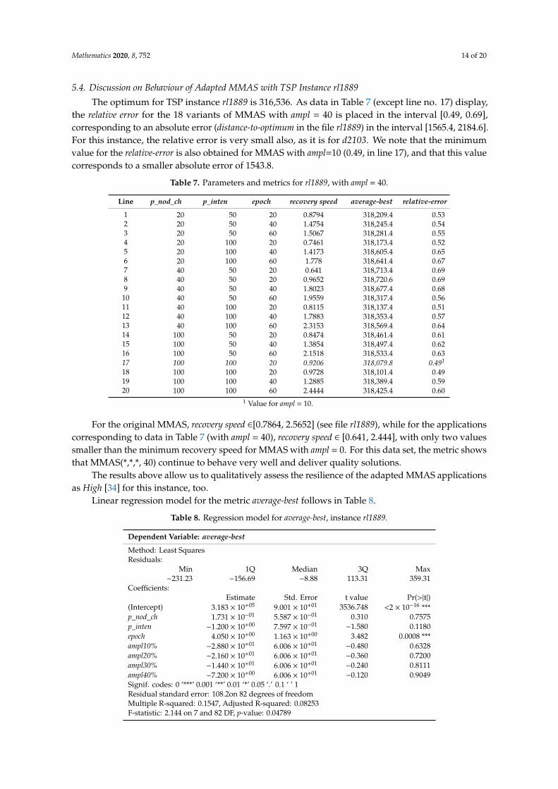
5.4. Discussion on Behaviour of Adapted MMAS with TSP Instance rl1889
The optimum for TSP instance rl1889 is 316,536. As data in Table 7 (except line no. 17) display, the relative error for the 18 variants of MMAS with ampl = 40 is placed in the interval [0.49, 0.69], corresponding to an absolute error (distance-to-optimum in the file rl1889) in the interval [1565.4, 2184.6]. For this instance, the relative error is very small also, as it is for d2103. We note that the minimum value for the relative-error is also obtained for MMAS with ampl=10 (0.49, in line 17), and that this value corresponds to a smaller absolute error of 1543.8.
Table 7. Parameters and metrics for rl1889, with ampl = 40.
Line p_nod_ch p_inten epoch recovery speed average-best relative-error 1 20 50 20 0.8794 318,209.4 0.53 2 20 50 40 1.4754 318,245.4 0.54 3 20 50 60 1.5067 318,281.4 0.55 4 20 100 20 0.7461 318,173.4 0.52 5 20 100 40 1.4173 318,605.4 0.65 6 20 100 60 1.778 318,641.4 0.67 7 40 50 20 0.641 318,713.4 0.69 8 40 50 20 0.9652 318,720.6 0.69 9 40 50 40 1.8023 318,677.4 0.68
10 40 50 60 1.9559 318,317.4 0.56 11 40 100 20 0.8115 318,137.4 0.51 12 40 100 40 1.7883 318,353.4 0.57 13 40 100 60 2.3153 318,569.4 0.64 14 100 50 20 0.8474 318,461.4 0.61 15 100 50 40 1.3854 318,497.4 0.62 16 100 50 60 2.1518 318,533.4 0.63 17 100 100 20 0.9206 318,079.8 0.491
Figure 2. Intercorrelations between the path-performance metricsaverage-best, stddev-best, best try andworst try for fl3795.
Mathematics 2020, 8, 752 14 of 20
5.4. Discussion on Behaviour of Adapted MMAS with TSP Instance rl1889The optimum for TSP instance rl1889 is 316,536. As data in Table 7 (except line no. 17) display,
the relative error for the 18 variants of MMAS with ampl = 40 is placed in the interval [0.49, 0.69],corresponding to an absolute error (distance-to-optimum in the file rl1889) in the interval [1565.4, 2184.6].For this instance, the relative error is very small also, as it is for d2103. We note that the minimumvalue for the relative-error is also obtained for MMAS with ampl=10 (0.49, in line 17), and that this valuecorresponds to a smaller absolute error of 1543.8.
Table 7. Parameters and metrics for rl1889, with ampl = 40.
Line p_nod_ch p_inten epoch recovery speed average-best relative-error
1 20 50 20 0.8794 318,209.4 0.532 20 50 40 1.4754 318,245.4 0.543 20 50 60 1.5067 318,281.4 0.554 20 100 20 0.7461 318,173.4 0.525 20 100 40 1.4173 318,605.4 0.656 20 100 60 1.778 318,641.4 0.677 40 50 20 0.641 318,713.4 0.698 40 50 20 0.9652 318,720.6 0.699 40 50 40 1.8023 318,677.4 0.6810 40 50 60 1.9559 318,317.4 0.5611 40 100 20 0.8115 318,137.4 0.5112 40 100 40 1.7883 318,353.4 0.5713 40 100 60 2.3153 318,569.4 0.6414 100 50 20 0.8474 318,461.4 0.6115 100 50 40 1.3854 318,497.4 0.6216 100 50 60 2.1518 318,533.4 0.6317 100 100 20 0.9206 318,079.8 0.491
18 100 100 20 0.9728 318,101.4 0.4919 100 100 40 1.2885 318,389.4 0.5920 100 100 60 2.4444 318,425.4 0.60
1 Value for ampl = 10.
For the original MMAS, recovery speed ∈[0.7864, 2.5652] (see file rl1889), while for the applicationscorresponding to data in Table 7 (with ampl = 40), recovery speed ∈ [0.641, 2.444], with only two valuessmaller than the minimum recovery speed for MMAS with ampl = 0. For this data set, the metric showsthat MMAS(*,*,*, 40) continue to behave very well and deliver quality solutions.
The results above allow us to qualitatively assess the resilience of the adapted MMAS applicationsas High [34] for this instance, too.
Linear regression model for the metric average-best follows in Table 8.
Table 8. Regression model for average-best, instance rl1889.
Dependent Variable: average-best
Method: Least SquaresResiduals:
Min 1Q Median 3Q Max−231.23 −156.69 −8.88 113.31 359.31
Coefficients:Estimate Std. Error t value Pr(>|t|)
(Intercept) 3.183 × 10+05 9.001 × 10+01 3536.748 <2 × 10⁻¹⁶ ***p_nod_ch 1.731 × 10−01 5.587 × 10−01 0.310 0.7575p_inten −1.200 × 10+00 7.597 × 10−01 −1.580 0.1180epoch 4.050 × 10+00 1.163 × 10+00 3.482 0.0008 ***ampl10% −2.880 × 10+01 6.006 × 10+01 −0.480 0.6328ampl20% −2.160 × 10+01 6.006 × 10+01 −0.360 0.7200ampl30% −1.440 × 10+01 6.006 × 10+01 −0.240 0.8111ampl40% −7.200 × 10+00 6.006 × 10+01 −0.120 0.9049Signif. codes: 0 ‘***’ 0.001 ‘**’ 0.01 ‘*’ 0.05 ‘.’ 0.1 ‘ ’ 1Residual standard error: 108.2on 82 degrees of freedomMultiple R-squared: 0.1547, Adjusted R-squared: 0.08253F-statistic: 2.144 on 7 and 82 DF, p-value: 0.04789

Mathematics 2020, 8, 752 15 of 20
Considering the adjusted R-Squared index we conclude that the linear regression model doesnot explain the average-best dependence of epoch, p_nod_ch, p_inten, ampl. As in the case of d2103, theimplementation performs very well for every combination of parameters.
For the metric recover speed, the linear regression model is presented in Table 9.
Table 9. Regression model for recovery speed, instance rl1889.
Dependent Variable: recovery speed
Method: Least SquaresResiduals:
Min 1Q Median 3Q Max−0.59491 −0.12230 −0.00215 0.12432 0.56298
Coefficients:Estimate Std. Error t value Pr(>|t|)
(Intercept) 0.2704582 0.1120153 2.414 0.018 *p_nod_ch 0.0010162 0.0006953 1.462 0.148p_inten 0.0007799 0.0009454 0.825 0.412epoch 0.0275353 0.0014473 19.025 <2 × 10⁻¹⁶ ***ampl10% −0.0380889 0.0747408 −0.510 0.612ampl20% −0.0471611 0.0747408 −0.631 0.530ampl30% −0.0201778 0.0747408 −0.270 0.788ampl40% −0.0285889 0.0747408 −0.383 0.703Signif. codes: 0 ‘***’ 0.001 ‘**’ 0.01 ‘*’ 0.05 ‘.’ 0.1 ‘ ’ 1Residual standard error: 0.2242 on 82 degrees of freedomMultiple R-squared: 0.8166, Adjusted R-squared: 0.801F-statistic: 52.17 on 7 and 82 DF, p-value: <2.2 × 10⁻¹⁶
This model indicates a negative correlation of the metric recovery speed with ampl and positivecorrelations with p_nod-ch, p_inten and epoch. As for the case of instance d2103, only the factors epochand ampl are significant in the model.
In Figure 3 we chose to display the same type of correlogram as in Figure 1, in order to comparethe intercorrelations of other time-performance metrics for d2103 and rl1889.
Mathematics 2020, 8, x FOR PEER REVIEW 16 of 21
ampl10% −0.0380889 0.0747408 −0.510 0.612 ampl20% −0.0471611 0.0747408 −0.631 0.530 ampl30% −0.0201778 0.0747408 −0.270 0.788 ampl40% −0.0285889 0.0747408 −0.383 0.703 Signif. codes: 0 '***' 0.001 '**' 0.01 '*' 0.05 '.' 0.1 ' ' 1 Residual standard error: 0.2242 on 82 degrees of freedom Multiple R-squared: 0.8166, Adjusted R-squared: 0.801 F-statistic: 52.17 on 7 and 82 DF, p-value: < 2.2 × 10⁻¹⁶
This model indicates a negative correlation of the metric recovery speed with ampl and positive correlations with p_nod-ch, p_inten and epoch. As for the case of instance d2103, only the factors epoch and ampl are significant in the model.
In Figure 3 we chose to display the same type of correlogram as in Figure 1, in order to compare the intercorrelations of other time-performance metrics for d2103 and rl1889.
Figure 3. Correlogram of the time-performance metrics avg.time-best, stddev-best, stddev.time best, average-iterations, better_solutions and number of epochs for rl1889.
We notice the same types of correlations for d2103 as for rl1889, except for average-iterations and stddev.time best, for which the correlation is positive for d2103 and negative for rl1889. For rl1889, the order parameter [84] is OP = 0.5129.
6. Discussion
The statistical analysis of data recorded for two of the studied TSP instances (d2103 and rl1889) reveals that the adapted MMAS implementation is highly resilient: both the delivered solutions and the time-performance metrics show that the ant algorithms perform very well when distortions appear. For these two instances, under the settings presented in Section 4.2, the quality of the solutions returned by MMAS(epoch, p_nod_ch, p_inten, ampl) do not depend on the four factors, while the recovery speed depends on epoch and ampl. These facts, supported by the statistical analysis of the experimental data, allow us to conclude that the applications are highly resilient. For the other TSP instance, fl3795, the adapted MMAS also proves to be resilient, but with a different behavior pattern: the quality of the solutions returned is slightly influenced by epoch and ampl, while the recovery
Figure 3. Correlogram of the time-performance metrics avg.time-best, stddev-best, stddev.time best,average-iterations, better_solutions and number of epochs for rl1889.

Mathematics 2020, 8, 752 16 of 20
We notice the same types of correlations for d2103 as for rl1889, except for average-iterations andstddev.time best, for which the correlation is positive for d2103 and negative for rl1889. For rl1889, theorder parameter [84] is OP = 0.5129.
6. Discussion
The statistical analysis of data recorded for two of the studied TSP instances (d2103 and rl1889)reveals that the adapted MMAS implementation is highly resilient: both the delivered solutions andthe time-performance metrics show that the ant algorithms perform very well when distortions appear.For these two instances, under the settings presented in Section 4.2, the quality of the solutions returnedby MMAS(epoch, p_nod_ch, p_inten, ampl) do not depend on the four factors, while the recovery speeddepends on epoch and ampl. These facts, supported by the statistical analysis of the experimentaldata, allow us to conclude that the applications are highly resilient. For the other TSP instance, fl3795,the adapted MMAS also proves to be resilient, but with a different behavior pattern: the quality ofthe solutions returned is slightly influenced by epoch and ampl, while the recovery speed does notdepend on the four factors. The answer to the question “Why does this happen?” could be searchedamong multiple causes, but two are immediate: the number of nodes and the instances of structures.These will drive our next studies: one focused on larger instances and another based on the structuralfeatures [85] of TSP instances. The nondeterministic nature of MMAS can also suggest that research onanother output data set, for the same instances, is worth being investigated.
Our previous research with ACO [86,87] gave us some insight on the ant algorithms behaviorunder different circumstances. When referring to the resilience attributes synthesized in [34], wenotice that all of them are representative for this class of algorithms. A brief enumeration of resilienceattributes (and their translation to ACO and the artificial ants) include: interconnection among theagents (artificial ants communicate, which leads to system flexibility); redundancy of units (artificialants perform the same simple tasks, but the performance of the system emerges from their interaction);diversity and variety in resilient systems, which means that there are different parts and a variety ofways of functioning (all these features have been implemented in ACO); the diversity of approaches,which is about generating various views on a situation (also possible in ACO). Moreover, parallelismand distributiveness (implicit in ACO, with no central command and no single point of failure) andhandling of increased workloads (easily achievable with ACO), dynamic learning (the pheromoneupdating mechanism) are important attributes. Finally, self-organization lies in the natural model thatinspired ACO and further developments of this heuristic approach.
When optimization problems arise in practice, the users need to have confidence in the quality ofthe solutions provided by their applications. There are many situations when things do not go “bythe book”. Sometimes unexpected events happen and change the graph representation of a problem,or make some data unavailable. Other demanding situations can emerge when communication isinterrupted, data are imprecise or mistaken, or even human errors appear. In such cases, if applicationsare resilient, these manage to provide solutions which are sufficiently close to those provided in normalconditions. Ant algorithms are systems that behave in a manner that is widely accepted by researchersand practitioners as resilient. One goal for our future work would be the design of ant algorithmsthat embed other types of intelligence and are able to learn and adapt. This falls into line with theinnovative proposal of Florio [88]: “ . . . we need to look at the nature and change the paradigm ofresilience from «being at work while staying the same» to «being at work while getting better», namelybecoming a better system or being”.
Author Contributions: Conceptualization, methodology, writing—original draft preparation, writing—reviewand editing, E.N., G.C.C., L.B.I.; software, G.C.C.; formal analysis, visualization, Y.H.; investigation, E.N., G.C.C.,L.B.I.; project administration, funding acquisition, E.N. All authors have read and agreed to the published versionof the manuscript.

Mathematics 2020, 8, 752 17 of 20
Funding: The research performed by E.N., G.C.C., and the APC were funded by the Ministry of Educationand Research, through the National Council for the Financing of Higher Education, Romania, grantnumber CNFIS-FDI-2019-0453.
Conflicts of Interest: The authors declare no conflict of interest. The funders had no role in the design of thestudy; in the collection, analyses, or interpretation of data; in the writing of the manuscript, or in the decision topublish the results.
References
1. Fiskel, J. Designing resilient, sustainable systems. Environ. Sci. Technol. 2003, 37, 5330–5339. [CrossRef]2. Arthur, W. Complexity and the economy. Science 1999, 284, 107–109. [CrossRef] [PubMed]3. Starr, R.; Newfrock, J.; Delurey, M. Enterprise resilience: Managing risk in the network economy. Strategy
Bus. 2004, 30, 1–10. Available online: https://www.strategy-business.com/article/8375?gko=9ee65 (accessedon 19 March 2020).
4. Folke, C.; Carpenter, S.; Elmquist, T.; Gunderson, L.; Holling, C.; Walker, B. Resilience and sustainabledevelopment: Building adaptive capacity in a world of transformations. Ambio 2002, 31, 437–440. [CrossRef]
5. Lal, R. Sustainable land use systems and soil resilience. In Soil Resilience and Sustainable Land Use; Greenland, D.,Szabolcs, I., Eds.; CAB International: Wallingford, UK, 1994; pp. 41–67.
6. Gunderson, L.H. Ecological Resilience—In Theory and Application. Annu. Rev. Ecol. S 2000, 31, 425–439.[CrossRef]
7. Standish, R.J.; Hobbs, R.J.; Mayfield, M.M.; Bestelmeyer, B.T.; Suding, K.N.; Battaglia, L.L.; Eviner, V.;Hawkes, C.V.; Temperton, V.M.; Cramer, V.A.; et al. Resilience in ecology: Abstraction, distraction, or wherethe action is? Biol. Conserv. 2014, 177, 43–51. [CrossRef]
8. Bonnano, G. Loss, trauma, and human resilience: Have we underestimated the human capacity to thriveafter extremely aversive events? Am. Psychol. 2004, 59, 20–28. [CrossRef]
9. Rutter, M. Implications of Resilience Concepts for Scientific Understanding. Ann. N.Y. Acad. Sci. 2006.[CrossRef]
10. Beery, A.K.; Kaufer, D. Stress, social behaviour, and resilience: Insights from rodents. Neurobiol. Stress 2015,1, 116–127. [CrossRef]
11. Adger, W. Social and ecological resilience: Are they related? Progr. Hum. Geogr. 2000, 24, 347–364. [CrossRef]12. Calloway, D.E.; Newman, M.E.J.; Strogatz, S.H.; Watts, D.J. Network Robustness and Fragility: Percolation
on Random Graphs. Phys. Rev. Lett. 2000, 85, 5468–5471. [CrossRef] [PubMed]13. Adler, C.O.; Dagli, C.H. Study of the Use of a Genetic Algorithm to Improve Networked System-of-Systems
Resilience. Procedia Comput. Sci. 2014, 36, 49–56. [CrossRef]14. Sha, Z.; Panchal, J. Towards the design of complex evolving networks with high robustness and resilience.
Procedia Comput. Sci. 2013, 16, 522–531. [CrossRef]15. Trivedi, K.S.; Kim, D.D.; Ghosh, R. Resilience in computer systems and networks. In Proceedings of the 2009
International Conference on Computer-Aided Design (ICCAD’09), San Jose, CA, USA, 2–5 November 2009.[CrossRef]
16. Matni, N.; Leong, Y.P.; Wang, Y.S.; You, S.; Horowitz, M.B.; Doyle, J.C. Resilience in Large Scale DistributedSystems. Procedia Comput. Sci. 2014, 28, 285–293. [CrossRef]
17. Yu, D.J.; Rao, P.S.; Klinkhamer, C.; Krueger, E.H.; Sangwan, N.; Sung, K. Aligning Different Schools ofThought on Resilience of Complex Systems and Networks. IRGC Resource Guide on Resilience v29-07-20162016, Lausanne: EPFL International Risk Governance Center. Available online: https://www.irgc.org/
riskgovernance/resilience/ (accessed on 19 March 2020).18. Ford, R.; Carvalho, M.; Mayron, L.; Bishop, M. Towards Metrics for Cyber Resilience. In Proceedings of the
21st EICAR Annual Conference Proceedings, Lisbon, Portugal, 7–8 May 2012; pp. 151–159.19. Omer, A.; Mostashari, A.; Lindemann, U. Resilience Analysis of Soft Infrastructure Systems. Procedia Comput.
Sci. 2014, 28, 565–574. [CrossRef]20. Cutter, S.L.; Barnes, L.; Berry, M.; Evans, E.; Tate, E.; Webb, J. A place-based model for understanding
community resilience to natural disasters. Glob. Environ. Change 2008, 18, 598–606. [CrossRef]21. Jordan, E.; Javernick-Will, A. Measuring Community Resilience and Recovery: A Content Analysis of
Indicators. Constr. Res. Congr. 2012, 2190–2199. [CrossRef]

Mathematics 2020, 8, 752 18 of 20
22. Scott, J. Architecting Resilient Systems: Accident Avoidance and Survival and Recovery from Disruptions; WileySeries in Systems Engineering and Management; John Wiley and Sons: Hoboken, NJ, USA, 2010.
23. MacAskill, K.; Guthrie, P. Multiple interpretations of resilience in disaster risk management. Procedia Econ.Financ. 2014, 18, 667–674. [CrossRef]
24. Chien, A.; Baaji, P.; Beckman, P.; Dun, N.; Fang, A.; Fujita, H.; Iskra, K.; Rubenstein, Z.; Zheng, Z.; Schreiber, R.;et al. Versioned Distributed Arrays for Resilience in Scientific Applications: Global View Resilience. ProcediaComput. Sci. 2015, 51, 29–38. [CrossRef]
25. Wright, C.; Kiparoglou, V.; Williams, M.; Hilton, J. A Framework for Resilience Thinking. Procedia Comput.Sci. 2012, 8, 45–52. [CrossRef]
26. Bruneau, M.; Reinhorn, A. Overview of the Resilience Concept. In Proceedings of the 8th US NationalConference on Earthquake Engineering, San Francisco, CA, USA, 18–22 April 2006; p. 2040.
27. Proag, V. The concept of vulnerability and resilience. Procedia Econ. Financ. 2014, 18, 369–376. [CrossRef]28. Bahill, T.A.; Botta, R. Fundamental Principles of Good Systems Design. Eng. Manag. J. 2008, 20, 9–17.
[CrossRef]29. Sols, A. Increasing Systems Resilience through the Implementation of a Proactive Technology Refreshment
Program. Procedia Comput. Sci. 2014, 28, 26–33. [CrossRef]30. Alsberg, A.P.; Day, J.D. A principle for resilient sharing of distributed resources. In Proceedings of the ICSE
’76: 2nd International Conference on Software Engineering, San Francisco, CA, USA, 13–15 October 1976;Yeh, R.T., Ramamoorthy, C.V., Eds.; IEEE Computer Society Press: Washington, DC, USA, 1976; pp. 562–570.
31. Avizienis, A.; Laprie, J.C.; Randell, B.; Landwehr, C. Basic Concepts and Taxonomy of Dependable andSecure Computing. IEEE Trans. Dependable Secure Comput. 2004, 1, 11–33. [CrossRef]
32. Axelrod, C.W. Investing in Software Resiliency. J. DefenseSoftw. Eng. 2009, 22, 20–25.33. Marcus, E.; Stern, H. Blueprints for High Availability: Designing Resilient Distributed Systems; John Wiley &
Sons: New York, NY, USA, 2000.34. Chandra, A. Synergy between Biology and Systems Resilience. Master’s Thesis, Missouri University of Science
and Technology, Rolla, MO, USA, 2010. Available online: https://scholarsmine.mst.edu/masters_theses/6728(accessed on 19 March 2020).
35. Duijnhoven, H.; Neef, M. Framing Resilience. From a model-based approach to management process.Procedia Econ. Financ. 2014, 18, 425–430. [CrossRef]
36. Proag, V. Assessing and measuring resilience. Procedia Econ. Financ. 2014, 18, 222–229. [CrossRef]37. Li, L.; Peng, H.; Kurths, J.; Yang, Y.; Schellnhuber, H.J. Chaos-order transition in foraging behavior of ants.
Proc. Natl. Acad. Sci. USA 2014, 111, 8392–8397. [CrossRef]38. Chittka, L.; Muller, H. Learning, specialization, efficiency and task allocation in social insects. Commun.
Integr. Biol. 2009, 2, 151–154. [CrossRef]39. Morgan, E.D. Trail pheromones of ants. Physiol. Entomol. 2009, 34, 1–17. [CrossRef]40. Dorigo, M.; Maniezzo, V.; Colorni, A. The Ant System: Optimization by a colony of cooperating agents. IEEE
Trans. Syst. Man Cybern. Part B 1996, 26, 1–13. [CrossRef] [PubMed]41. Dorigo, M.; Gambardella, L.M. Ant Colonies for the Traveling Salesman Problem; Technical Report
TR/IRIDIA/1996-3; Université Libre de Bruxelles: Brussels, Belgium, 1996.42. Dorigo, M.; Di Caro, G. The Ant Colony Optimization Meta-Heuristic. New Ideas in Optimization; McGraw-Hill:
New York, NY, USA, 1999.43. Applegate, D.L.; Bixby, R.E.; Chvátal, V.; Cook, W.J. The Traveling Salesman Problem: A Computational
Study. In Princeton Series in Applied Mathematics; Princeton University Press: Princeton, NJ, USA, 2011.44. Cook, W.J. Pursuit of the Traveling Salesman: Mathematics at the Limits of Computation; Princeton University
Press: Princeton, NJ, USA, 2012.45. Dantzig, G.B.; Fulkerson, R.; Johnson, S.M. Solution of a Large-Scale Traveling Salesman Problem. Oper. Res.
1954, 2, 393–410. [CrossRef]46. Karp, R.M. Reducibility among Combinatorial Problems. In Complexity of Computer Computations; The IBM
Research, Symposia; Miller, R.E., Thatcher, J.W., Eds.; Plenum Press: New York, NY, USA, 1972; pp. 85–103.47. Woeginger, G.J. Exact Algorithms for NP-Hard Problems: A Survey. In Combinatorial Optimization—Eureka,
You Shrink! Lecture Notes in Computer, Science; Jünger, M., Reinelt, G., Rinaldi, G., Eds.; Springer:Berlin/Heidelberg, Germany, 2003; Volume 2570, pp. 185–207. [CrossRef]

Mathematics 2020, 8, 752 19 of 20
48. Held, M.; Karp, R.M. The Traveling-Salesman Problem and Minimum Spanning Trees. Oper. Res. 1970, 18,1138–1162. [CrossRef]
49. Held, M.; Karp, R.M. The Traveling-Salesman Problem and Minimum Spanning Trees: Part II. Math. Program.1971, 1, 6–25. [CrossRef]
50. Concorde TSP Solver. Available online: http://www.math.uwaterloo.ca/tsp/concorde/ (accessed on 19March 2020).
51. Rojanasoonthon, S.; Bard, S.F.; Reddy, S.D. Algorithms for parallel machine scheduling: A case study of thetracking and data relay satellite system. J. Oper. Res. Soc. 2003, 54, 806–821. [CrossRef]
52. Ratliff, H.D.; Rosenthal, A.S. Order-Picking in a Rectangular Warehouse: A Solvable Case for the TravellingSalesman Problem. Oper. Res. 1983, 31, 507–521. [CrossRef]
53. Grötschel, M.; Jünger, M.; Reinelt, G. Optimal Control of Plotting and Drilling Machines: A Case Study.Math. Method Oper. Res. 1991, 35, 61–84. [CrossRef]
54. Lee, J.Y.; Shin, S.Y.; Park, T.H.; Zhang, B.T. Solving traveling salesman problems with DNA moleculesencoding numerical values. Biosystems 2004, 78, 39–47. [CrossRef]
55. Grover, L. Local search and the local structure of NP-complete problems. Oper. Res. Lett. 1992, 12, 235–243.[CrossRef]
56. Codenotti, B.; Margara, L. Traveling Salesman Problem and Local Search. Appl. Math. Lett. 1992, 5, 69–71.[CrossRef]
57. Gamboa, D.; Rego, C.; Glover, F. Data Structures and Ejection Chains for Solving Large Scale TravelingSalesman Problems. Eur. J. Oper. Res. 2005, 160, 154–171. [CrossRef]
58. Lin, S.; Kernighan, B.W. An Effective Heuristic Algorithm for the Traveling-Salesman Problem. Oper. Res.1973, 21, 498–516. [CrossRef]
59. Applegate, D.; Cook, W.J.; Rohe, A. Chained Lin-Kernighan for large traveling salesman problems. INFORMSJ. Comput. 2003, 15, 82–92. [CrossRef]
60. Kirkpatrick, S.; Gelatt, C.D., Jr.; Vecchi, M.P. Optimization by Simulated Annealing. Science 1983, 220, 671–680.[CrossRef] [PubMed]
61. Zhou, A.H.; Zhu, L.P.; Hu, B.; Deng, S.; Song, Y.; Qiu, H.; Pan, S. Traveling-Salesman-Problem AlgorithmBased on Simulated Annealing and Gene-Expression Programming. Information 2019, 10, 7. [CrossRef]
62. Scholz, J. Genetic Algorithms and the Traveling Salesman Problem. A Historical Review. In Proceedingsof the MInf Seminar at the Dept. of Computer Science of the Hamburg University of Applied Sciences,Winter 2017/2018, Hamburg, Germany. Available online: https://arxiv.org/pdf/1901.05737.pdf (accessed on 19March 2020).
63. Dorigo, M.; Birattari, M.; Stutzle, T. Ant Colony Optimization. IEEE Comput. Intell. Mag. 2006, 1, 28–39.[CrossRef]
64. Stützle, T. ACOTSP Software. 2004. Available online: https://www.swmath.org/software/11237 (accessed on19 March 2020).
65. Costa, Y.J.; Castaño, N.; Betancur, J.F. Optimization based on Multi-type Ants for the Traveling SalesmanProblem. In Proceedings of the 9th Computing Colombian Conference (9CCC), Pereira, Colombia, 3–5September 2014; IEEE Press: New York, NY, USA, 2014; pp. 144–149.
66. Holzinger, A.; Plass, M.; Kickmeier-Rust, M.; Holzinger, K.; Crisan, G.C.; Pintea, C.M.; Palade, V. Interactivemachine learning: Experimental evidence for the human in the algorithmic loop. Appl. Intell. 2019, 49,2401–2414. [CrossRef]
67. Jovanovic, R.; Tuba, M. Ant Colony Optimization Algorithm with Pheromone Correction Strategy for theMinimum Connected Dominating Set Problem. Comput. Sci. Inf. Syst. 2013, 10, 133–149. [CrossRef]
68. Lopez-Ibáñez, M.; Stützle, T. An Analysis of Algorithmic Components for Multiobjective Ant ColonyOptimization: A Case Study on the Biobjective TSP. In Lecture Notes in Computer Science; Artifical Evolution.EA; Collet, P., Monmarché, N., Legrand, P., Schoenauer, M., Lutton, E., Eds.; Springer: Berlin/Heidelberg,Germany, 2009; Volume 5975. [CrossRef]
69. López-Ibáñez, M.; Stützle, T. Automatically improving the anytime behaviour of optimisation algorithms.Eur. J. Oper. Res. 2014, 235, 569–582. [CrossRef]

Mathematics 2020, 8, 752 20 of 20
70. Dorigo, M. Optimization, Learning and Natural Algorithms. Ph.D. Thesis, Dipartimento di Elettronica,Politecnico di Milano, Milan, Italy, 1991. (In Italian)
71. Dorigo, M.; Maniezzo, V.; Colorni, A. Positive Feedback as a Search Strategy; Technical Report 91-016;Dipartimento di Elettronica, Politecnico di Milano: Milan, Italy, 1991.
72. Dorigo, M.; Stützle, T. The Ant Colony Optimization Metaheuristic: Algorithms, Applications, and Advances.In Handbook of Metaheuristics. International Series in Operations Research & Management Science; Glover, F.,Kochenberger, G.A., Eds.; Springer: Boston, MA, USA, 2003; Volume 57. [CrossRef]
73. Stützle, T.; Hoos, H.H. MAX-MIN Ant System. Future Gener. Comput. Syst. 2000, 16, 889–914. [CrossRef]74. Data Files and Statistical Analysis Files for d2013, fl3795 and rl1889. Available online: http://cadredidactice.
ub.ro/ceraselacrisan/2d-euclidean-tsp-instances/ (accessed on 1 March 2020).75. Crisan, G.C.; Nechita, E.; Palade, V. Ant-Based System Analysis on the Traveling Salesman Problem under
Real-World Settings. In Combinations of Intelligent Methods and Applications. Smart Innovation, Systems andTechnologies; Hatzilygeroudis, I., Palade, V., Prentzas, J., Eds.; Springer: Berlin/Heidelberg, Germany, 2016;Volume 46, pp. 39–59. [CrossRef]
76. TSPLIB. Available online: http://comopt.ifi.uni-heidelberg.de/software/TSPLIB95/ (accessed on 1 March 2020).77. Discrete and Combinatorial Optimization, Universität Heidelberg Institut für Informatik. Available online:
http://comopt.ifi.uni-heidelberg.de/software/TSPLIB95/ (accessed on 19 March 2020).78. Jünger, M.; Reinelt, G.; Rinaldi, G. The Traveling Salesman Problem. The Institute for Systems Analysis and
Computer Science, Rome, Technical Report R375. 1994. Available online: http://www.iasi.cnr.it/reports/R375/
R375.pdf (accessed on 16 April 2020).79. Johnson, D.S.; McGeoch, L.A. The Traveling Salesman Problem: A Case Study. In Local Search in Combinatorial
Optimization; Aarts, E.H.L., Lenstra, J.K., Eds.; Princeton University Press: Princeton, NJ, USA; Oxford, UK,2003; pp. 215–310. [CrossRef]
80. Birattari, M.; Dorigo, M. How to assess and report the performance of a stochastic algorithm on a benchmarkproblem: Mean or best result on a number of runs? Optim. Lett. 2007, 1, 309–311. [CrossRef]
81. Jackson, S. System Resilience: Capabilities, Culture and Infrastructure. In Proceedings of the INCOSEInternational Symposium, San Diego, CA, USA, 24–28 June 2007; Wiley Online Library, 2014; Volume 17,pp. 885–899. [CrossRef]
82. Tamvakis, P.; Xenidis, Y. Resilience in Transportation Systems. Procedia Soc. Behav. Sc. 2012, 48, 3441–3450.[CrossRef]
83. Crisan, G.C. Ant Algorithms in Artificial Intelligence. Ph.D. Thesis, Al.I. Cuza University of Iasi, Iasi,Romania, 2008.
84. Cheeseman, P.; Kanefsky, B.; Taylor, W.M. Where the really hard problems are. In Proceedings of the IJCAI’91:12th International Joint Conference on Artificial Intelligence, Sydney, Australia, 24–30 August 1991; MorganKaufmann Publishers: Burlington, MA, USA, 1991; Volume 1, pp. 331–337. [CrossRef]
85. Nallaperuma, S.; Wagner, M.; Neumann, F. Analyzing the effects of instance features and algorithm parametersfor Max–Min Ant System and the Traveling Salesperson Problem. Front. Robot AI 2015, 2. [CrossRef]
86. Czibula, G.; Crisan, G.C.; Pintea, C.M.; Czibula, I.G. Soft Computing Approaches on the Bandwidth Problem.Informatica 2013, 24, 169–180. [CrossRef]
87. Pintea, C.M.; Crisan, G.C.; Chira, C. Hybrid ant models with a transition policy for solving a complexproblem. Logic. J. IGPL 2012, 20, 560–569. [CrossRef]
88. De Florio, V. Systems, Resilience, and Organization: Analogies and Points of Contact with Hierarchy Theory.In Proceedings of the 4th International Workshop on Computational Antifragility and Antifragile Engineering(ANTIFRAGILE 2017), Trieste, Italy, 3–6 July 2017; Available online: https://arxiv.org/abs/1411.0092 (accessedon 20 April 2020).
© 2020 by the authors. Licensee MDPI, Basel, Switzerland. This article is an open accessarticle distributed under the terms and conditions of the Creative Commons Attribution(CC BY) license (http://creativecommons.org/licenses/by/4.0/).