ANNALES DE LA FACULTÉ DES SCIENCES DE TOULOUSE

B. BONNARD

E. TRÉLATOn the role of abnormal minimizers in sub-riemannian geometryAnnales de la faculté des sciences de Toulouse 6e série, tome 10, no 3(2001), p. 405-491.<http://www.numdam.org/item?id=AFST_2001_6_10_3_405_0>

© Université Paul Sabatier, 2001, tous droits réservés.

L’accès aux archives de la revue « Annales de la faculté des sciencesde Toulouse » (http://picard.ups-tlse.fr/~annales/), implique l’accord avecles conditions générales d’utilisation (http://www.numdam.org/legal.php).Toute utilisation commerciale ou impression systématique est constitu-tive d’une infraction pénale. Toute copie ou impression de ce fichierdoit contenir la présente mention de copyright.

Article numérisé dans le cadre du programmeNumérisation de documents anciens mathématiques

http://www.numdam.org/

- 405 -

On the role of abnormal minimizers insub-Riemannian geometry (*)

B. BONNARD, E. TRÉLAT (1)

Annales de la Faculte des Sciences de Toulouse Vol. X, n° 3, 2001pp. 405-491

RESUME. - On considere un probleme sous-Riemannien (U, D, g) of Uest un voisinage de 0 dans D une distribution lisse de rang 2 et gune metrique lisse sur D. L’objectif de cet article est d’expliquer le roledes geodesiques anormales minimisantes en geometric SR. Cette analyseest fondee sur le modele SR de Martinet.

ABSTRACT. - Consider a sub-Riemannian geometry (U, D, g) where U isa neighborhood at 0 in D is a rank-2 smooth (COO or CW) distributionand g is a smooth metric on D. The objective of this article is to explainthe role of abnormal minimizers in SR-geometry. It is based on the analysisof the Martinet SR-geometry.

1. Introduction

Consider a smooth control system on Rn : :

where the set of admissible controls U is an open set of bounded measurablemappings u defined on [0, T(u)] ~ and taking their values in We fix

q(0) = qo and T(u) - T and we consider the end-point mapping E : u E

U ~---~ q(T, qo, u), where q(t, qo, u) is the solution of (1) associated to u E Uand starting from qo at t = 0. We endow the set of controls defined on [0, T]with the L°°-topology. A trajectory q(t, qo ic) denoted in short q is said tobe singular or abnormal on [0, T] if ic is a singular point of the end-pointmapping, i.e, the Frechet derivative of E is not surjective at S.

~ * ~ Re~u le 2 juin 1999, accepte le 9 juillet 2001(1) Universite de Bourgogne, LAAO, B.P. 47870, 21078 Dijon Cedex, France.

e-mail: bbonnard@u-bourgogne.fr, trelat@topolog.u-bourgogne.fr

Consider now the optimal control problem : min fo fO (q( t), u(t))dt,where f ° is smooth and q(t) is a trajectory of (1) subject to boundaryconditions : q (o) E M0 and q(T) E M1, where Mo and lVh are smooth sub-manifolds of According to the weak maximum principle [37], minimizingtrajectories are among the singular trajectories of the end-point mapping ofthe extended system in :

and they are solutions of the following equations :

where Hv = p, f (q, u) > -f-v f ° (q, u) is the pseudo-Hamiltonian, p is theadjoint vector, , > the standard inner product in Rn and v is a constantwhich can be normalized to 0 or -1/2. Abnormal trajectories correspondto v = 0 ; their role in the optimal control problem has to be analyzed.Their geometric interpretation is clear : if C denotes the set of curves so-

lutions of (1), they correspond to singularities of this set and the analysisof those singularities is a preliminary step in any minimization problem.This problem was already known in the classical calculus of variations, seefor instance the discussion in [8] and was a major problem for post-secondwar development of this discipline whose modern name is optimal control.The main result, concerning the analysis of those singularities in a generic

m

context and for affine systems where f(q, u) = Fo(q) + are givenz=i

in [12] and [5]. The consequence of this analysis is to get rigidity resultsabout singular trajectories when m = 1, that is under generic conditions asingular trajectory q joining qo = ~y(o) to ql = ) is the only trajectorycontained in a C°-neighborhood joining qo to qi in time T (and thus isminimizing).

In optimal control the main concept is the value function S defined asfollows. If qo, ql and T are fixed and ~y is a minimizer associated to u.y and

joining qo to qi in time T, we set :

The value function is solution of Hamilton-Jacobi-Bellman equation andone of the main questions in optimal control is to understand the role ofabnormal trajectories on the singularities of S.

The objective of this article is to make this analysis in local sub-Rieman-nian geometry associated to the following optimal control problem :

subject to the constraints :

q E U C IR,n, where {Fi, -" , are m linearly independant vector fieldsgenerating a distribution D and the metric g is defined on D by taking the

as orthonormal vector fields. The length of a curve q solution of (4)on [0, T] and associated to u E U is given by : L(q) = / T ~ u2 (t) 1/2 dtand the SR-distance between qo and qi is the minimum of the length ofthe curves q joining qo to ql . The sphere r) with radius r is the setof points at SR-distance r from qo. If any pairs qo, ql can be joined by aminimizer, the sphere is made of end-points of minimizers with length r. Itis a level set of the value function.

It is well known (see [1]) that in SR-geometry the sphere S(qo, r) withsmall radius r has singularities. For instance they are described in [4] in thegeneric contact situation in R3 and they are semi-analytic. Our aim is togive a geometric framework to analyze the singularities of the sphere in theabnormal directions and to compute asymptotics of the distance in thosedirections. We analyze mainly the Martinet case extending preliminary cal-culations from [2, 10]. The calculations are intricate because the singularitiesare not in the subanalytic category even if the distribution and the metricsare analytic. Moreover they are related to similar computations to evaluatePoincaré return mappings in the Hilbert’s 16th problem (see ~35,, 38]) usingsingular perturbation techniques.

The organization and the contribution of this article is the following.

In Sections 2 and 3 we introduce the required concepts and recall someknown results from [6, 7, 12] to make this article self-contained.

In Section 2, we compute the singular trajectories for single-input affinecontrol systems : q = Fo (q), using the Hamiltonian formalism. Thenwe evaluate under generic conditions the accessibility set near a singulartrajectory to get rigidity results and to clarify their optimality status in SRgeometry.

In Section 3 we present some generalities concerning SR geometry.

In Section 4 we analyze the role of abnormal geodesics in SR Martinetgeometry. We study the behaviour of the geodesics starting from 0 in theabnormal direction by taking their successive intersections with the Mar-tinet surface filled by abnormal trajectories. This defines a return mapping.To make precise computations we use a gradated form of order 0 where theMartinet distribution is identified to Ker w, w = dz - the Martinet

surface to y = 0, the abnormal geodesic starting from 0 to t ’2014~ (t, 0, 0) andthe metric is truncated at : g = (1 + + (1 + ,~x + where

a, are real parameters. The geodesics equations project onto the planarfoliation : :

where c = 2014= is a small parameter near the abnormal direction which

projects onto the singular points 8 = Here the Martinet plane y = 0 isprojected onto a section ~ given by :

Equation (5) represents a perturbed pendulum ; to evaluate the trace ofthe sphere S(0, r) with the Martinet plane we compute the return mappingassociated to the section ~. Near the abnormal direction the computationsare localized to the geodesics projecting near the separatrices of the pendu-lum.

In order to estimate the asymptotics of the sphere in the abnormal direc-tion we use the techniques developped to compute the asymptotic expansionof the Poincare return mapping for a one-parameter family of planar vectorfields. This allows to estimate the number of limit cycles in the Hilbert’s16th problem, see [38]. Our computations split into two parts :

1. A computation where we estimate the return mapping near a saddle

point of the pendulum and which corresponds to geodesics close tothe abnormal minimizer in Cl -topology.

2. A global computation where we estimate the return mapping alonggeodesics visiting the two saddle points and which corresponds togeodesics close to the abnormal minimizer in C° -topology, but not inC1-topology (see [42] for a general statement).

Our results are the following.

e If /3 = 0, the pendulum is integrable and we prove that the spherebelongs to the log-exp category introduced in ~19~, and we computethe asymptotics of the sphere in the abnormal direction.

e If /3 ~ 0, we compute the asymptotics corresponding to geodesics C~close to the abnormal one.

We end this Section by conjecturing the cut-locus in the generic Martinetsphere using the Liu-Sussmann example [29].

The aim of Section 5 is to extend our previous results to the general caseand to describe a Martinet sector in the n-dimensional SR sphere.

First of all in the Martinet case the exponential mapping is not properand the sphere is tangent to the abnormal direction. We prove that thisproperty is still valid if the abnormal minimizer is strict and if the sphereis C1-stratifiable.

Then we complete the analysis of SR geometry corresponding to sta-ble 2-dimensional distributions in by analyzing the so-called tangentialcase. We compute the geodesics and make some numerical simulations andremarks about the SR spheres.

The flat Martinet case can be lifted into the Engel case which is a

left-invariant problem of a 4-dimensional Lie group. We give an uniformparametrization of the geodesics using the Weierstrass function. Both Heisen-berg case and Martinet flat case can be imbedded in the Engel case.

The main contribution of Section 5 is to describe a Martinet sector inthe SR sphere in any dimension using the computations of Section 4. We usethe Hamiltonian formalism (Lagrangian manifolds) and microlocal analysis.This leads to a stratification of the Hamilton-Jacobi equation viewed in thecotangent bundle.

Acknoledgments. - We thank M. Chyba for her numerical simulationsconcerning the sphere.

2. Singular or abnormal trajectories

2.1. Basic facts

Consider the smooth control system :

and let q(t) be a trajectory defined on [0, T~ and associated to a controlu E U. If we set :

the linear system :

is called the linearized or variational system along (q, u). It is well known,see [12] that the Frechet derivative in L°°-topology of the end-point mappingE is given by :

where $ is the matricial solution of : &#x26; = = id.

Hence (q, u) is singular on [0, T] if and only if there exists a non-zero vec-tor p orthogonal to Im E’(u), that is the linear system (8) is not controllableon [0, T~ .

If we introduce the row vector : p(t) - (t) , a standard com-putation shows that the triple (q, p, u) is solution for almost all t E [0, T] ofthe equations :

which takes the Hamiltonian form :

where H(q, p, u) _ p, f(q, u) > . The function H is called the Hamiltonianand p is called the adjoint vector.

This is the parametrization of the singular trajectories using the maxi-mum principle. We observe that for each t T[, the restriction of (q, u)is singular on [0, t] and at t the adjoint vector p(t) is orthogonal to the vec-tor space K(t) image of t] by the Fréchet derivative of the end-pointmapping evaluated on the restriction of u to [0, t~. . The vector space K(t)corresponds to the first order Pontryagin’s cone introduced in the proof ofthe maximum principle. If t T] we shall denote by k(t) the codimensionof K(t) or in other words the codimension of the singularity. Using the ter-minology of the calculus of variations k(t) is called the order of abnormality.

The parametrization by the maximum principle allows the computationof the singular trajectories. In this article we are concerned by systems ofthe form :

and the algorithm is the following.

2.2. Determination of the singular trajectories

2.2.1. The single input affine case

It is convenient to use Hamiltonian formalism. Given any smooth func-tion H on T * U, li will denote the Hamiltonian vector field defined by H.If Hi , H2 are two smooth functions, , H2 ~ will denote their Poissonbracket : : {H1, H2} = dH1 (H2). If X is a smooth vector field on U, we setH = p, X (q) > and H is the Hamiltonian lift of X If Xl, X2 are two vectorfields with Hi = p, Xi(q) >, i = 1, 2 we have : H2~ _ p, ~X1, X~~(q) >where the Lie bracket is : . [X1, X2](q) = (q)X2(q) - (q)X1(q). VVeshall denote by Ho == p, Fo (q) > and Hi = p, Fi (q) > . .

If f(q, u) = Fo (q) + uFl (q), the equation (9) can be rewritten :

for all t E [0, T]

We denote by z = (q, p) E T * U and let (z, u) be a solution of aboveequations. Using the chain rule and the constraint : Hi = 0, we get :

This implies : 0 = Ho ~ (z (t) ) for all t. Using the chain rule again w-eget :

This last relation enables us to compute u(t) in many cases and justifiesthe following definition :

DEFINITION 2.1. - For any singular curve (z, u) J = ~0, T~ ~---~ T * Ll xR, R(z, u) will denote the set ~t E J, ~ ~Ho, ~ . Tlm set

R(z, u) possibly empty is always an open subset of J.

DEFINITION 2.2. A singular trajectory (z, u) : J -~ T * U x R iscalled of order two if R(z, u) is dense in J

The following Proposition is straightforward :

PROPOSITION 2.1. - If (z, u) : J E--~ T*M x R is a singular trajectoryand R(z, u) is not empty then :

1. z restricted to R(z, u) is smooth ;

Conversely, let (Fo, Fl) be a pair a smooth vector fields such that theopen subset n of all z E T * U such that {{H0, H1}, H1(z) ~ 0 is not empty.

If H : 03A9 ~ R is the function H0 + {{H0, H1}, H0} {{H1, H0}, H1} H1 then any trajectory

of ii starting at t = 0 from the set Hi = - 0 is a singulartrajectory of order 2.

This algorithm allows us to compute the singular trajectories of minimalorder. More generally we can extend this computation to the general case.

DEFINITION 2.3. - For any multi-index a E ~0, cx = (a1, ... an)the function Ha is defined by induction by : Ha = A

singular trajectory (z, u) is said of order 1~ > 2 if all the brackets of orderk : H~, with {3 == ... , ~31 - 1 are 0 along z and there exists

a = (1, cx2, ... , such that Hal (z) is not identically 0.

The generic properties of singular trajectories are described by the fol-lowing Theorems of [13]. .

THEOREM 2.2. - There exists an open dense subset G of pairs of vectorfields (Fo, Fl ) such that for any couple (Fo, F’1 ) E G, the associated controlsystem has only singular trajectories of minimal order 2.

THEOREM 2.3. - There exists an open dense subset G1 in G such that

for any couple (Fo, Fl ) in G1, , any singular trajectory has an order of ab-normality equal to one. that is corresponds to a singularity of the end-pointmapping of codimension one.

2.2.2. The case of rank two distributions

Consider now a distribution D of rank 2. In SR-geometry we need tocompute singular trajectories t ~--~ q(t) of the distribution and it is notrestrictive to assume the following : t ~---~ q(t) is a smooth immersion. Thenlocally there exist two vector fields Fl, F2 such than D = Span {F1, F2}and moreover the trajectory can be reparametrized to satisfy the associatedaffine system :

where ul (t) - l. It corresponds to the choice of a projective chart on thecontrol domain.

Now an important remark is the following. If we introduce the Hamil-2

tonian lifts : Hi = p, Fi(q) > for i = 1, 2, and H = ~uiHi the singulartrajectories are solutions of the equations :

Here the constraints ~H ~u

= 0 means : H = 0 and H = 0 This leads tothe following definition :

DEFINITION 2.4. - Consider the affine control system : q = Fi + uF~.A singular trajectory is said exceptional if it is contained on the level set :H = 0, where H = p, Fi > +u p, F2 > is the Hamiltonian.

Hence to compute the singular trajectories associated to a distributionwe can apply locally the algorithm described in the affine case and keepingonly the exceptional trajectories. An instant of reflexion shows that thoseof minimal order form a subset of codimension one in the set of all singulartrajectories because H is constant along such a trajectory and the additionalconstraint Hi = 0 has to be satisfied only at time t = 0. Hence we have :

PROPOSITION 2.4. - The singular arcs of D are generically singulararcs of order 2 of the associated affine system. They are exceptional andform a subset of codimension one in the set of all singular trajectories.

2.3. Feedback equivalence

DEFINITION 2.5. - Consider the class S of smooth control systems ofthe form :

Two systems f(x, u) and f’(y, v) are called feedback equivalent if thereexists a smooth diffeomorphism of the form : ~ : (x, u) ~ (y, v), y = v = u) which transforms f into f’ :

and we use the notation f’ * f. .

Here we gave a global definition but there are local associated conceptswhich are :

e local feedback equivalence at a point (xo, uo) E Rn x Rm.e local feedback equivalence at a point xo of the state-space.e local feedback equivalence along a given trajectory : q(t) or (q(t), u(t))

of the system.

This induces a group transformation structure called the feedback group

G f on the set of such diffeomorphisms. For affine systems we consider a sub-group of G f which stabilizes the class. This leads to the following definition.

DEFINITION 2.6. - Consider the class of m-inputs affine control sys-tems :

,

m

where F(q)u = It is identified to the set = ~Fo, Fl, ... , i=l

of (m + 1)-uplets of vector fields. The vector field Fo is called the drift. LetD be the distribution defined by D = Span {Fi(?),... , We restrict

the feedback transformations to diffeomorphisms of the form ~ _ (cp(q),u) = a(q) + preserving the class A. We denote by G the set of

triples (w, a, ,~) endowed with the group structure induced by G f.

We observe the following : take (Fo. F) E A (~, a, (3) E G, thenthe image of (Fo, F) by 03A6 is the affine system (Fo, F’) given by :

In particular the second action corresponds to the equivalence of the twodistributions D and D’ associated to the respective systems.

The proof of the following result is straightforward, see [9].

PROPOSITION 2.5. . - The singular trajectories are feedback invariants.

Less trivial is the assertion that for generic systems, singular trajecto-ries will allow to compute a complete set of invariants, see [9] for such adiscussion.

2.4. Local classification of rank 2 generic distributions D in R3

We recall the generic classification of rank 2 distributions in see

[45], with its interpretation using singular trajectories. Hence we consider asystem :

q = (x, y, z). We set D = Span F~~ and we assume that D is of rank 2.Our classification is localized near a point qo E R3 and we can assume qo =0. We deal only with generic situations, that is all the cases of codimension~ 3. We have three situations which can be distinguished using the singulartrajectories.

Introducing Hi = p, Fi (q) >, i = 1, 2, a singular trajectory z = (q, p)must satisfy :

and hence they are contained in the set M : {q E R3 ; det (Fl, F2,F2~) - 0~ called the Martinet surface. The singular controls of order

2 satisfy :

We define the singular set S = S1~S2 where Si F2, [[Fi, F2] , Fi]) = 0}.We have the following situations.

Case 1. - Take a point qo ~ M, then through qo there passes no singulararc. In this case D is (C°° or isomorphic to Ker a, with a = ydx + dz.

For this normalization da = dy A dx (Darboux) and ~ ~z is the characteristicdirection. This case is called the contact case.

Case 2 (Codimension one). - We take a point qo E Since qo ~ S,we observe that AI is near qo a smooth surface. This surface is foliatedby the singular trajectories. A smooth (C°° or C03C9)-normal form is given

by D = Ker a, where Q = dz - In this normal form we have the

following identification :

e Martinet surface M : : y = 0.

2022 The singular trajectories are the solution of Z = d restricted toy = 0.

This case is called the Martinet case.

Case 3 (Codimension 3). - We take a point Xo E M n S and we as-sume that the point qo is a regular point of Al. The analysis of [45] showsthat in this case we have two different C~-reductions to a CW-normal form

depending both upon a modulus m. The two cases are : :

1. Hyperbolic case. D = Ker a, a = dy + (xy + x2z + In

this representation the Martinet surface is given by :

and the singular flow in M is represented in the (x, z) coordinatesby :

We observe that 0 is a resonant saddle and the parameter ~n is anobstruction to the C~-linearization.

2. Elliptic case. D = Ker a, a - dy + (xy ~- x3 + xz2 + 3The Martinet surface is here identified to :

in which the singular now is given by :

Hence 0 is a center and still m is an obstruction to C°°-linearization. The

analysis of [44] shows that the singularity is C°-equivalent to a focus.

We call the case 3 the tangential situation because D is tangent to theMartinet surface at 0. We must stress that it is not a simple singularity andmoreover there are numerous analytic moduli.

2.5. Accessibility set near a singular trajectory

The objective of this Section is to recall briefly the results of [12] whichdescribe geometrically the accessibility set near a given singular trajectorysatisfying generic assumptions (see also [42, 41~ ) .

2.5.1. Basic assumptions and definitions

We consider a smooth single input smooth afhne control system :

Let 03B3 be a reference singular trajectory corresponding to a control u Eand starting at t = 0 from ~y(0) - qo and we denote by (-y, p, u),

where p is an adjoint vector for the associated solution of the equations (9)from the maximum principle. We assume the following :

(H0) (~y, p) is contained in the set SZ = ~z = (q, p) ; ~ ~Ho, ~0~, ~y is contained in the set 0’ = {q ; X (q) and Y(q) are linearlyindependant} and moreover ~ : [0, T] ~ --~ U is one-to-one.

Then according to the results of Section 2.2, the curve z = (~y, p) is a

singular curve of order 2 solution of the Hamiltonian vector field H, withH = Ho + l H1. Moreover the trajectory -y : [0, T] ~ S2 ls

a smooth curve and 03B3 is a one-to-one immersion.

Using the feedback invariance of the singular trajectories we may assumethe following normalizations : u(t) = 0 for t E [0, T] and 03B3 can be taken asthe trajectory : t --~ (t, 0, 0, ... , 0). Since u is normalized to 0, by successivederivations of the constraints Hi = 0, i.e p(t), Fl (~y(t)) >= 0 for t E [0, T~,we get the relations :

where Vk is the vector field and is defined recursively by :

It is well known, see [21], [23], that for t > 0 the space E(t) =Span is contained in the first order Pontryagin’s coneK(t) evaluated along -y. We make the following assumptions :

(Hl) For t E [0, t], the vector space E(t) is of codimension one and gener-ated by ~v°(~y(t)), ... , V~n-2~(-~(t))~.

(H2) If 7~ ~ 3, for each t E ~0, T~, X (-y(t)) ~ Span ~V°{-y(t)), ... , , yn-3)(’Y(t))~

DEFINITION 2.7. - Let (~y(t), p(t), u(t)) be the reference trajectory de-fined on [0, T~ and assume that the previous assumptions (HO), (H1), (H2)

are satisfied. According to (Hl) the adjoint vector p is unique up to ascalar. The Hamiltonian is H = H0+uH1 along the reference trajectory and

Hi = 0. If H = 0, we say that -y is G-exceptional. Let D = ~ ~u d2 dt2 ~H ~u =

p( ), [[F1, Fo], F1](03B3(t)) > . The trajectory, is said G-hyperbolic if H.D > 0along q and G-elliptic if H.D 0 along ~y.

Remark 2.1. According to the higher-order maximum principle thecondition 0 called the Legendre-Clebsch condition is a time opti-mality necessary condition, see [23].

2.5.2. Semi-normal forms

The main tool to evaluate the end-point mapping is to construct semi-normal forms along the reference trajectory ~y using the assumptions(H0, H1, H2) and the action of the feedback group localized near ~y. Theyare given in [12] and we must distinguish two cases.

PROPOSITION 2.6. - Assume that, is a G-hyperbolic or elliptic tra-jectory. Then the system is feedback equivalent in a C0-neighborhood of 03B3to a system (No, Nl ) with : :

where an,n is strictly positive (resp. negative) on [0, T] if 03B3 is elliptic (resp.

hyperbolic) and R = f is a vector field such that the weight of Ri

has order greater or equal to 2 (resp. 3) for i = 2, ... , n - 1 (resp. i = 1),the weights of the variables qi being 0 for i = 1, and 1 for i = 2, ... , n.

Geometric interpretation :

. The reference trajectory -y is identified to t ~ (t, 0, ... 0) and theassociated control is u = 0. In particular ~ 1 .

qi~. We have :

(iii) adz N1.No = 8qniand the first order Pongryagin’s cone along q is : ~f~ = ~ 2014~-,... , ~ .g Y g g ’Y ~.y

I ~ ,

The linearized system is autonomous and in the Brunovsky canonicalform : = (~,... , = u.

. The adjoint vector associated to 03B3 is p = (E, 0,... , 0) where £ = +1 inthe elliptic case in the hyperbolic case, the Hamiltonianbeing E.

. The intrinsic second-order derivative of the end-point mapping isidentified along 1 to :

with c~2 = ... , = ~n = u and the boundary conditions

at s = 0 and T : 03C62(s) = ... = 03C6n(s) = 0.PROPOSITION 2.7. - Let ~y be a G-exceptional trajectory. Then n > 3

and there exists a C0-neighborhood of 03B3 in which the system is feedbackequivalent to a system (No, Nl) with : :

where an-l,n-1 is strictly positive on [0, T] and R = Ri V 2 . , Rn-1 = 0

is a vector field such that the weight of Ri has order greater or equal to 2(resp. 3) for i = 1, ... , n

- 2 (resp. i = n)J the weights of the variables q2being zero for i = 1, ; one for i = 2, ... , n - 1 and two for qn. .

Geometric interpretation

. The reference trajectory ~y is identified to t ~----~ (t, 0, ... , 0) and theassociated control is u - 0.

. We have the following normalizations :

(ii) Noi - adn-2 1 ’

(iii) ad2 N1.N0 = ~2 N1 ~qn-12

and the first order Pontryagin’s cone along 1 is

In the exceptional case tangent to The linearized system along ~ is the system : (~ = ~~,... , =

. The adjoint vector p associated to 03B3 can be normalized to p = (0,...,0,-1).

. The intrinsic second-order derivative of the end-point mapping along~ is identified to :

with : rj;l = 03C62,...,n-2 - , n - u and the boundary condi-

tions at s = 0 and T : = ... = = 0.

2.5.3. Evaluation of the accessibility set near,

We consider all trajectories q(t, u) of the system starting at time t = 0from ~y(o) - 0 ; the accessibility set at time t is the set : : A(o, t) - U

uELf

q(t, u). It is the image of the end-point mapping.

We use our semi-normal forms to evaluate the accessibility set for alltrajectories of the system contained in a C°-neighborhood of -y. We havethe following, see [12] for the details.

Hyperbolic-elliptic situation

By truncating the semi-normal form and replacing ql by t we get alinear-quadratic model :

and it can be integrated in cascade.

Let 0 t T and fix the following boundary conditions : q(0) =0 and : : q2 (t) = ... ~ = = qn(t) = 0, we get a projection of theaccessibility set A( 0, t) in the line ql which describes the singularity of theend-point mapping evaluated on u(s) = 0 for t. Fig. 1 representsthis projection when t varies.

Figure 1

Geometric interpretation The reference trajectory q is

minimal (resp. time maximal) in the hyperbolic case (resp. elliptic case) upto a time tic which corresponds to a first conjugate time 0 along, forthe time minimal (resp. time maximal) control problem.

In particular we get the following Proposition :

PROPOSITION 2.8. - Assume T Then the reference singular tra-jectory 03B3 defined on [0, T] is in the hyperbolic (resp. elliptic) case the onlytrajectory y contained in a CO -neighborhood and satisfying the boundaryconditions : y(0) = ~y(o), _ q(T) in a time T T (resp. T > T). .

This property is called CO -one-side rigidity, compare with ~5~.

Exceptional caseWe proceed as before. The model is :

Let 0 T and consider the following boundary conditions :

?(0) = 0 and = t, ~(~) = ... = = 0. We get a projection ofthe accessibility set ~4(0~) on the line It is represented on Fig. 2.

Figure 2

Geometric interpretation The reference trajectory q is

optimal up to a time t1cc which corresponds to a first conjugate time t1cc >0. In particular we have the following result.

PROPOSITION 2.9. - Assume T t1cc. Then the reference singularexceptional trajectory ~y is CO -isolated (or CO -rigid).

2.5.4. Conclusion : : the importance of singular tra jectories in op-timal control

The previous analysis shows that singular trajectories play generically

an important role in any optimal control problem : Min T0 f °{x, u)dt whenthe transfert time T is fixed. Indeed they are locally the only trajectoriessatisfying the boundary conditions and hence are optimal. If the transferttime T is not fixed only exceptional singular trajectories play a role. Infact as observed by [5] they correspond to the singularities of the timeextended end-point mapping : E : (T, u) ~--~ q(T, x°, u). It is the situation

encountered in sub-Riemannian geometry.

3. Generalities about sub-Riemannian geometry

From now on, we work in the C"’-category.

DEFINITION 3.1. - A SR-manifold is defined as a n-dimensional man-ifold M together with a distribution D of constant rank m ~ n and a

Riemannian metric 9 on D. An admissible curve t ’2014~ q(t), 0 ~ t T is anabsolutely continuous curve such that q(t) E D (q (t) ) B ~0 ~ for almost everyt. The length and the energy of q are respectively defined by :

where ( , ) is the scalar product defined by g on D. The SR-distance be-tween qo, ql E M denoted dsR (qo, ql ) is the infimum of the lengths of theadmissible curves joining qo to qi .

3.1. Optimal control formulation

The problem can be locally restated as follows. Let qo E AI and choosea coordinate system (U, q) centered at qo such that there exist rrz (sinooth)vector fields ~Fl, ... which form an orthonormal basis of D. Theneach admissible curve t -~ q(t) on U is solution of the control system :

The length of a curve does not depend on its parametrization, henceevery admissible curve can be reparametrized into a lipschitzian curves ~--~q(s) parametrized by arc-length : : (q(s), q(s)) = 1, see ~29~.

If an admissible curve on U : t ~--~ T is parametrized byarc-length we have almost everywhere :

and L(q) = fo (~ 262)1/2 dt = T. Hence the length minimization problemis equivalent to a time-optimal problem for system ( 11 ) . This problem is not

m

convex because of the constraints : 2:u; = 1, but it is well-known that thei=l

problem is equivalent to a time optimal control problem with m

constraints : ~u2 (t) 1.2=1

It is also well-known that if every curve is parametrized on a in-terval [0, T~, the length minimization problem is equivalent to minimization problem.

Introducing the extended control system :

and the end-point mapping E of the extended system : u E U ~--~ q(t, u, qo) ,q = (q, qO), q(o) _ (qo, 0), from the maximum principle the minimizers canbe selected among the solutions of the maximum principle :

m m

where H == p, > is the pseudo-Hamiltonian and p =i=l i=l

(p, po) e is the adjoint vector of the extended system. From theprevious equation t ~--~ Po(t) is a constant which can be normalized to 0

m m

or -1/2. Introduce Hv = p, > where v = 0 or -1/2 ;i=1 i=1

then the previous equations are equivalent to :

The solutions of these equations correspond to the singularities of theend-point mapping of the extended system and are called geodesics in theframework of SR-geometry.

They split into two categories according to the following definition.

DEFINITION 3.2. - A geodesic is said to be abnormal if v = 0, and nor-mal if v = -1/2. Abnormal geodesics are precisely the singular trajectoriesof the original system (11).

A geodesic is called strict if the extended adjoint vector (p, po - v) is

unique up to a scalar, that is corresponds to a. singularity of codimensionone of the extended end-point mapping.

3.2. Computations of the geodesics

3.2.1. Abnormal case

They correspond to v = 0, and are the singular trajectories of sys-m

tem (11). The system is symmetric and hence H = uiPi, with Pi = i=l

p, Fi(q) > . Therefore they are exceptional. When m = 2, they are com-puted using the algorithm of Section 2. The case m > 2 will be excluded inour forthcoming analysis because from [5] in order to be optimal a singulartrajectory must satisfy the following conditions, known as Goh’s conditions :

dv, w E Vt E [0, T] and Fu denotes 03A3 uiFi. If m = 2, this reducesto the condition P2 ~ - 0 deduced from the conditions Pi = P2 = 0but if m > 2 it is a very restrictive condition which should not be generic(conjecture [21]).

3.2.2. Normal case

They correspond to v = -1/2. If the system of the Fi’s is orthonormal

then - 0 and hence ui - Pi 2 and Hv reduces to Hn _ - 1 The

trajectories parametrized by arc length are on the level set Hn = 1/2 andthe normal geodesics are solutions of the following Hamiltonian differentialequations : :

On the domain chart U, we can complete the m-vector fields {Fi,... , toform a smooth frame {Fi,... , , Fn ~ of T U. The SR-metric g can be extendedinto a Riemannian metric by taking the system of the Fi’s as an orthonormalframe. We set Pi = p, Fi (q) > for i = l, ... n and let P = (Pl , ~ ~ ~ , Pn ) .In the coordinate system (q, P) the normal geodesics are solutions of thefollowing equations :

We observe that _ p, [Fi,Fj](q) > and since the F2’s form aframe we can write :

where the cfj’s are smooth functions.

3.3. Exponential mapping - Conjugate and cut loci

Assume that the curves are parametrized by arc-length. If t !2014~ q(t) isany geodesic, the first point where q(.) ceases to be minimizing is called acut-point and the set of such points when we consider all the geodesics with

q (0) = qo will form the cut-locus L(qo).

The sub-Riemannian sphere with radius r > 0 is the set ,5’{qo, r) ofpoints which are at SR-distance r from qo. The wave front of length r isthe set W(qo r) of end-points of geodesics with length r starting from qo IfDA.L. (qo) is of rank n where DA.L is the Lie algebra generated by D, thenaccording to Filippov’s existence Theorem [27] if r is small enough each

point of distance r from qo is the end-point of a minimizing geodesic and

,S’(qo, r) is a subset of W {qo, r). We fix qo E U and let (q(t, qo,Po),p(t, qo,Po))be the normal geodesic, solution of (15) and starting from (qo, po) at t = 0.The exponential mapping is the

m

Its domain is the set C x R where C is ~po ; ; qo) = l~. If m n

i=l

it is a (non compact) cylinder contrarily to the Riemannian case m = n,where it is a sphere.

A conjugate point along a, normal geodesic is defined as follows. Let

(po tl ) with tl > 0 be a point is not an immersion. Then tl is

called a conjugate time along the normal geodesic and the image is calleda conjugate point. The conjugate locus C(qo) is the set of first conjugatepoints.

3.4. Gradated normal form

3.4.1. Adapted and priviliged coordinate system

Let (U, q) be a coordinate system centered at qo, with D - Span, ... , F~.,.L ~ . Assume that D satisfies the rank condition on U. We de-

fine recursively : Do = ~ 0~ = D and for p > 2 DP = Span +Hence DP is generated by Lie brackets of the Fi ’s with length

~ p. At p we have an increasing sequence of vector sub-spaces : ~0~ -D° {q) C C ... ~ C where r(q) is the smallest integer such that

(q) = TqU.

DEFINITION 3.3. - We say that qo is a regular point if the integersnp(q) = dim DP(q) remain constant for q in some neighborhood of qo Oth-erwise we say that qo is a singular point. Consider now a coordinate system(ql, , ... qn) such that dq~ vanishes identically on (qo) and doesn’tvanish identically on for some integer . Such a coordinate sys-tem is said to be adapted to the flag and the integer w~ is the weight of .

DEFINITION 3.4. - Consider now a SR-metric (D, g) defined on thechart ( U, q) and represented locally by the orthonormal vector fields

{~i~... , , F~.,2 ~ If f is a germ of smooth function at qo, the order of f at qois : :

(i) if f (qo) ~ 0, ~{f ) _ 0, ~(~) _

( ii ) otherwise : ~c, ( f ) - inf ~ p / ~ Y1, ... Vp E ~ Fl , ... with LYl o... o Lv~ ( f ) (qo ) ~ 0~ where Lv denotes the Lie derivative. The germf is called privileged if ~c ( f = min~ p ; df(DP (q° ) ) ~ 0) . A coordinatesystem ~ql, ... is said to be privileged if all the coordinates qiare privileged at qo.

We have the following very important estimation, see [7], [25] : :

PROPOSITION 3.1. - If (M, D, g) is a SR-manifold there exists a priv-ileged coordinate system q at every point qo - 0 of M. If wi is the order

(or weight) of the coordinate q~ we have the following estimation for theSR-distance :

DEFINITION 3.5. Let (U, q) be a privileged coordinate system for theSR-structure given locally by the m-orhonormal vector fields : {F1, ... , Fm}.

If w is the weight of qj, the weight of a

. is taken by convention as -wj.g q ’ g aq~

y

Every vector field Fi can be expanded into a Taylor series using the previousgradation and we denote by Fi the homogeneous term with lowest order- 1. The polysystem ~ Fl , ... is called the principal part of the SR-structure.

We have the following result, see [7]. .

PROPOSITION 3.2. . - The vector fields Fi i = l, ... , m generate a nilpo-tent Lie algebra which satisfies the rank condition. This Lie algebra is inde-pendant of the privileged coordinate system.

3.4.2. Gauge classification

Given a local SR-geometry (U, D, g) represented as the optimal controlproblem :

there exists a pseudo-group of transformations called the gauge group whichis the subgroup of the feedback group defined by the following transforma-tions :

(i) germs of diffeomorphisms ~; : q f--~ Q on U, preserving qo ; ;

(ii) feedback transformations u = preserving the metric g i.e,E 8(m, IR,) (orthogonal group).

The invariants of the associated classification problem are the geodesics.They split into two categories : abnormal geodesics which are feedback in-variants and normal geodesics.

If q is an adapted coordinate system, a gradated normal form of orderp > -1 is the polysystem ~Fp, ... , Fm~ obtained by truncating the vec-tor fields FZ at order p using the weight system defined by the adaptedcoordinates.

4. The role of abnormal minimizers in SR Martinet geometry

In this Section we analyze the role of abnormal minimizers in SR Mar-tinet geometry which is the prototype of the generic rank 2 situation. Beforeto present this analysis it is important to make a short visit to the contactsituation in JR 3.

4.1. The contact situation in R3

The contact situation in R3 has been analyzed in details in several ar-ticles [3, 4]. This analysis is based on computations about the exponentialmapping using a gradated normal form. To understand the remaining of thisarticle it is important to make the contact situation fit into the followingframework.

First, without losing any generality we can use to understand a genericcontact SR-problem a gradated form of order 1 computed in [4] where theSR-metric is defined by the two orthonormal vector fields : Fl, F2 where :

where Q is a quadratic form ~ + 2&#x26;.r?/ + depending on 3 parameters.The weight of .r, y is one and the weight of z is two. When a = 6 = c = 0,it corresponds to the contact situation of order -1 which is the well-knownHeisenberg case but also a gradated normal form o/ order 0.

To get an adapted frame we complete Fi , ~2 by ~3 = 2014. Computing we~

~

get: [Fi , ~2] = (1+2Q)~-. Using ~ = p, >, the geodesies equationsare :

’~

In the Heisenberg case we have Q = 0, and if we set P3 = A we get :fii + = 0, which is a linear pendulum.

Using the cylindric coordinates : Pi = sin B, P2 - sin 8, P3 - ~, whereB 7~ k7r, the geodesics parametrized by arc-length are solutions of the follow-ing equations :

where A is a constant. The important behavior is when ~ -~ oo. We mayassume A > 0. By making the following reparametrization : :

the angle equation takes the trivial form : de

= 1. Hence it is integrableand we obt ain B ( s ) = s + 00.

The remaining equations take the form :

For large a, they can be integrated as follows. We set ~ = 1/03BB : small

parameter, :r = ~X, ?/ = ~Y, z = ~ Z, 1 2 = 1 -f- Q - 1 ~- Ax2 ~- 2Bxy ~

~- ~ ~ ~ and vve

The previous equations can be integrated by quadratures by setting :

and we get in particular

The solutions are computed in the s-parametrization and the arc-length tcan be computed by integrating (19) by quadratures.

If we want to mimic this procedure in the Martinet situation, we shall en-counter integrability obstructions due to the existence of abnormal geodesics.

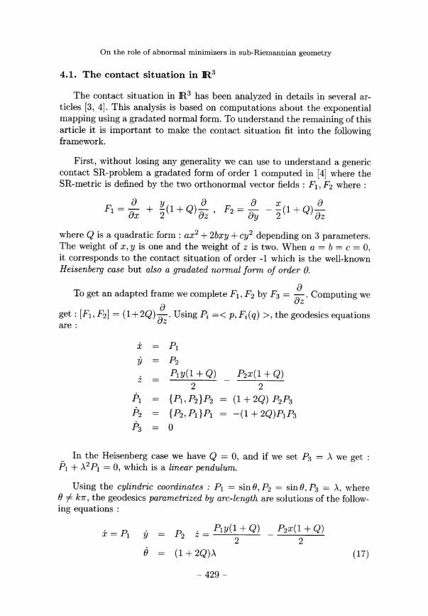
The sphere in the flat contact situation is represented on Fig. 3.

Figure 3. - SR sphere in the flat contact case

4.2. The Martinet situation

4.2.1. Normal forms and invariants

The Martinet SR-geometry is rather intricate and it is difficult to makea priori normalizations. It will appear later that a good starting point tomake the computations is to use the following normal form computed in [2] : :

. The distribution D is taken in the Martinet-Zhitomirski normal form :

. The metric on D is taken as a sum of squares + c(q)dy2.

In this representation the Martinet surface containing the abnormal geodesicsis the plane : y = 0 and the abnormal geodesics are the straight-lines : z = zo .The abnormal line passing through 0 is given by q : t ~ (~t, 0, 0).

The computations in [2] show that we can make an additional normaliza-tion on the metric by taking either the restriction of a or c to the Martinetplane y = 0 equal to 0.

The variables are gradated according to the following weights : the weightof x, y is one and the weight of z is three. By identifying by convention atorder p two normal forms where the Taylor series of a and c coincide atorder p we end up with the following representatives of order 0 :

either

In each of those representations the three parameters are, up to sign ; invari-ants. They can be used to compute the exponential mapping in the genericsituation. If we truncate g to dx2 + dy2 it corresponds to the principal partof order -1 of the SR-structure defined previously. In the sequel it will becalled the flat case.

4.2.2. Geodesics equations

The distribution D is generated by :

and the metric is given by g = adx2 + cdy2. We introduce the frame :

> for z == 1,2,3, i.e

First, we assume that g is not depending on z ; ; this is the case forthe gradated normal form of order 0. It corresponds to an isoperimetric

situation, ’ that is the existence of a vector field Z identified here to ~ ~ztransverse at 0 to D(0) and the metric g does not depend on z.

The system is written :

and the Hamiltonian associated to normal geodesics is :

and the geodesics controls are :

Normal geodesics are solutions of the following equations :

In the (q, P) representation the previous equations take the form :

If we parametrize by arc-length and if we introduce the cylindric co-ordinates : Pi = cos B, P2 - sin 8, P3 - ~, we end up with the followingequations :

It is proved in [11] that for a generic SR-problem, each geodesic is strict.In our representation we have the following result.

LEMMA 4.1. - The abnormal geodesic : t ~ (±t, 0, 0) is strict ifand only if the restriction of ay to the Martinet plane y = 0 is 0.

Using the gradated normal form of order 0 with the normalizations :

the equations (22) reduce to :

The previous equation defines a foliation (.F) of codimension one in

the plane (~/,~). Indeed using the parametrization : ~/a V~ ~ = T" anddenoting ’ the derivative with respect to T, the equations can be written : 1

and they can be projected onto the plane (y, e). The last two equations areequivalent to :

This equation will be used in the sequel to study the SR-Martinet geom-etry in the generic case of order 0. Unfortunately it depends on the choiceof coordinates. Note that in the flat case where a = c = 1 the equationreduces to 8" + A sin 03B8 = 0 which is a nonlinear pendulum.

4.2.3. Conservative case

The analysis of Subsection 4.1 shows that in the contact case the equa-tion (17) associated to the evolution of 0 defines an integrable foliation. Inthe Martinet case the foliation defined by equation (25) is not in generalintegrable. This leads to the following definition which is independant of thechoice of coordinates.

DEFINITION 4.1. - Let e(t, 0, A) be a normal geodesic parametrized byarc-length starting from ?(0) = 0 and associated to 0(0) = 00, P3 (o) - A.The problem is said conservative if there exists a coordinate y transverseto the Martinet surface such that for a dense set of initial conditions (00 , A)the trajectory t ---~ y(t) is periodic up to reparametrization. The equationdescribing the evolution of y is called the characteristic equation.

4.2.4. Analysis of the foliation .~

The foliation (.~) is described by equation (25) :

Moreover recall the relation : y’ = 9, 0’ 0+3 sin 0)

The singular line project onto 8 = k7r which correspond to the singular-ities of (25) : 0 = k7r, ()’ = 0.

Among the solutions of (25), only those satisfying the relation :

at T = 0 correspond to projections of geodesics starting at t - 0 fromq(0) = 0.

Using an energy-balance relation we can represent the solutions of (.~’)for [ A » ~ ,~ ~ ~y ~, see [10]. We may suppose A > 0. Introducing thesmall parameter : £ = and the parametrization s = 03BB we got theequation :

and equation (26) takes the form :

d28 ~!NThe flat case corresponds to cx = 03B2 = 0, i.e : ds2 -f- sin 8 = 0. _ () at

s = 0 and is also the limit case ~ ~ 0.

The following result is straightforward.

LEMMA 4.2. - The problem is conservative if and only if ,3 = U.

We represent below the trajectories of (,~’) for a » ~ a ~ , ~ ~3 ~ , ~ ~y ~ , onthe phase space : (8, 8) but geometrically it corresponds to a foliation onthe cylinder : : (eie, 8).

. Flat case (a = ~3 = 0). It corresponds to a pendulum, see Fig. 4.

Figure 4

The main properties are the following. We have two singularities :- 0 is a center.

- (7r, 0) is a saddle and the separatrix £ is a saddle connection.

Only the oscillating trajectories correspond to geodesics starting from 0.

. Conservative case (~3 = 0) The equation reduces to :

Multiplying both sides by 2014 and integrating on [0, ~] we get :6~

and the system has a global CW first integral : .’

The phase portrait is similar to the one in the flat case but the section

defined by (28) and corresponding 0 is here : de = ~03B1cos 8.ds

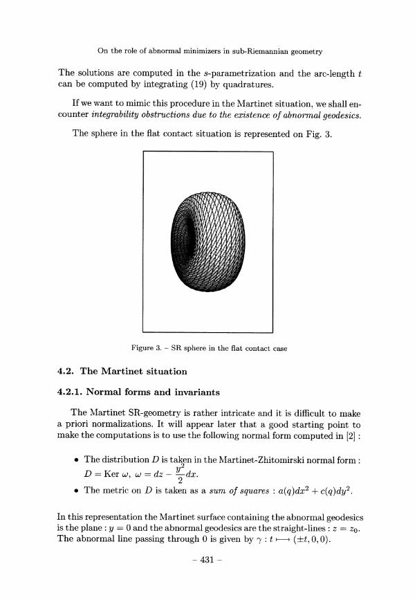
In particular if 0 (strict case) there exist both oscillating and ro-tating trajectories corresponding to projections of geodesics startingfrom 0, see Fig. 5.

Figure 5.-o;>0

. General case (,~ ~ 0) The two main differences are the following :- the center 0 becomes a focus ;- the saddle connection is broken.

The trajectories are represented on Fig. 6.The respective generic behaviors of t ~---~ y(t) are represented onFig. 7.It is important to observe that the behaviour of t f---~ y(t) is true forthe gradated form of order D; but also of any order when a ---~ oc.

4.2.5. Characteristic equation

If {3 = 0, the Hamiltonian Hn = 1 P2 i -~- P2 2) has two cyclic coordinates :x and z and therefore Px = cos 0(0) and pz = A are first integrals. The

equation H 1/2, with Pl /2 and P2 Py takes the form : .

Introducing : dr = - - it becomes :

Figure 6. - ,(3 > 0

Figure 7. - ;3 > 0

where a = (1 + ay) 2 Hence we get :

where F ( y) = ( 1-~- a~) 2 - ( px +P-=~/2)~. The analysis is based on the rootsof the quartic F(y). We assume ~ > 0.

We observe that F can be factorized as F1F2 with :

and we can write :

h 2 ~ 1 ~2 ,, 1 + ~2were: = 1 - px + §X ’ 2mI = 1 + PX §X

and: nt~ + nt" = I , 0.

~ - a , ~ - ~+-__=we can write :

m"F is a quartic whose roots on C are ~ = =bl , , 7? = =b m" .

m

The case m" - 0 is called critical and it corresponds to a double rootfor F. We have :

LEMMA 4.3. - In the strict case a ~ 0, there exist geodesics startingfrom 0 which are critical.

Geometric interpretationThe critical geodesics project in the (o, o) phase space onto a sepa-

ratrix, see Fig. 5.

The characteristic equation can be put into a normal form using anhomographic transformation to normalize the roots of F. The procedure isstandard, see [26]. We proceed as follows ; F is factorized into FlF2 and weconsider the pencil Fl + vF2 of two quadratic forms. If a ~ 0, there existtwo distinct real numbers vl, v2 such that Fl + vF2 is a perfect square :

Kl ( y - p) 2, I~2 ( y - ?)~. Using the homographic transformation :

the characteristic equation can be written in the normal form :

The right hand side corresponds to an integrand of an elliptic integral ofthe first kind. More precisely, excepted the critical case m" - 0, the solutiony in the u-coordinate can be computed as follows :

. if the quartic F admits two real roots, u can be parametrized using- the cn Jacobi function ;

. if the quartic F admits four real roots, u can be parametrized usingthe dn Jacobi function.

If a = 0, the analysis is simpler, indeed F(y) can be written :

where ~ = 03BBy 2k and ~ can be computed using only the cn function.PROPOSITION 4.4. - We have two cases : :

If 03B1 = 0, y = 2k 03BB~ where ~ is the cn Jacobi function.

(ii) If a ~ 0, y is generically the image by an homography of the cn ordn Jacobi function.

Geometric interpretation If a = 0, the motion of y is a cn whose

amplitude is 2k 03BB . The motion is symmetric with respect to y = 0 and theamplitude tends to 0 when A tends to the infinity, see Fig. 8.

If a ~ 0, we can expand : y = near u = 0. The motion of y is nou-1

more symmetric with respect to y = 0 and there is a shift. Hence y can beapproximated by a constant plus a cn or dn motion.

Figure 8. - c~ > 0

4.2.6. Integral formulas in the general conservative case

If the metric g does not depend on x, it is convenient to use the followingintegral formulas from [24] to compute x and z in terms of y.

We denote by e ( t ) t E [0, T ~ a normal geodesic starting from 0 and weassume that the component : t ~--~ y(t) oscillates periodically with period

P. We denote by 0 ti -" ~ tN T the successive times such thaty(ti) = 0. We introduce :

and we set :

Parametrizing the geodesics by y we must integrate the equations :

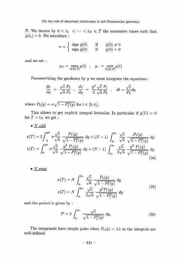
where P2 ( y ) _ ~ 1 - Pi ( y ) for t E [0, This allows to get explicit integral formulas. In particular if y (T ) = 0

for T = t N we get :

. N odd

. N even

and the period is given by :

The integrands have simple poles when Pl ( y) _ so the integrals arewell-defined.

4.2.7. The return mapping

The main geometric object to understand the role of abnormal trajecto-ries in the problem is the return mapping. Indeed if we consider the traceof the sphere and the wave front in the plane y = 0 :

S(0, r) = S(0, r) n (y = 0), , W(0, r) = W(O, r) n (y = 0) , ,they are in the image of the following mappings.

DEFINITION 4.2. - Let e : (t E ~0, T~, 8{0), ~1) f---~ {x{t), y(t), z(t)) bea normal geodesic, parametrized by arc-length. If y(t) ~ 0, we can define0 ti ... ~ tN T as the times corresponding to y(ti) - 0. The firstreturn mapping is :

and more generally the n-th return mapping is the map :

where Di are the domains.

If the length is fixed to r, we observe that W (o, r) is the union of the

image of the return mappings and (~r, 0) which are the end-points of theabnormal geodesics.

The remaining of this Section is devoted to the analysis of the returnmapping. We proceed by perturbations of the flat case. We shall estimatethe asymptotic expansions of ,S‘ and Y~’ in the abnormal direction. They arean union of curves in the plane. Such a curve is subanalytic if and onlyif it admits a Puiseux expansion. It is a practical criterion to measure thetranscendence of the sphere and wave front in the abnormal direction.

4.2.8. The pendulum and the elastica in the flat case

In the flat case the equation (27) is a simple pendulum :

where s = t is the arc-length parameter and y = - £ . . In particulars

if v (0) = 0 , We have fl/ = 0. We get:

The integration is standard using elliptic integrals [26]. The character-istic equation takes the form :

and we introduce k, [0,1] by setting :

where px = cos 0(0) . We = 20142014 and we get the equation :

We integrate with r~(o) = ~/(0) = 0 and we choose the branch ~j(o) > 0corresponding to (O) = sin 0(0) > 0. We get using the cn Jacobi function :

where 4I~(I~) is the period, K being the complete elliptic integral of the firstkind :

Hence

which coincides with the formula obtained by integrating the pendulum.

The components y and z can be computed by quadratures and we get :

where E is the complete elliptic integral of the second kind :

The previous parametrization corresponds to geodesics with A > 0, 8(0) E]0, 03C0[. The solutions corresponding to 03BB > 0, 8 (o) ~]-03C0, 0 are deduced usingthe symmetry : S1 : (z, y, z) ~ (x, -y, z) The solutions corresponding toA 0 are deduced using the symmetry : ,S’2 : (x, y, z) ~--~ (-x, y, -z). Thesolutions with A = 0 play no role in our analysis.

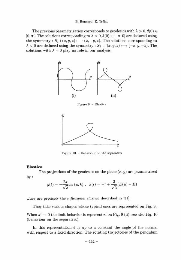
Figure 9. - Elastica

Figure 10. - Behaviour on the separatrix

ElasticaThe projections of the geodesics on the plane (x, y) are parametrized

by :

They are precisely the inflexional elastica described in [31].

They take various shapes whose typical ones are represented on Fig. 9.

When k’ -~ 0 the limit behavior is represented on Fig. 9 (ii), see also Fig. 10(behaviour on the separatrix).

In this representation 8 is up to a constant the angle of the normalwith respect to a fixed direction. The rotating trajectories of the pendulum

correspond to geodesics not starting from 0. They project on the space (x, y)onto non inflexional elastica, see Fig. 11 (ii).

Figure 11

4.2.9. Trace of ,S’(o, r) and W (o, r) in y = 0 in the flat case

The successive intersection times with y = 0 are given by : ti - 2K ,i = 1, ... , N. If we fix the length to ti = r, we get the following curves :

It represents a parametric curve, where the parameter is k e]0,1[. Usingthe relation : E(K + = (2i + 1)E we obtain for each z the followingcurves : k ’2014~ Ci(k) =

where k E~O,1 ~. We can easily draw those curves using the standard packageabout elliptic functions in Mathematica, see Fig. 12.

The exterior curve obtained for i = 1 represents the intersection of thesphere S(o, r) with the Martinet plane in the domain z > 0. Each pointof this curve is the end-point of two distinct minimizers and by obviousgeometric reasoning we have : :

PROPOSITION 4.5. - The cut locus L(o, r) is Cl U -Cl.

Moreover by inspecting Fig. 12 we deduce the following :

Figure 12

PROPOSITION 4.6. - The abnormal geodesics are minimizers.

This result is now new but here the proof is based on the analysis of thegeodesic flow. The main property is that at each intersection with y = 0, thevariable z has non zero drift which can be easily evaluated using (38). Thiswill lead to optimality results for the general metric; by stability.

This is an alternative proof to the optimality results presented in Section3 or in [5], [29], where we consider all the trajectories of the system.

Remark 4.1. We observe that (-r, 0) is a ramified point of the trace ofthe wave front on the Martinet plane with an infinite number of branches.This gives us a precise geometric interpretation on the structure of thegeodesics of fixed length with respect to the abnormal line. Indeed for everyneighborhood U of (-r, 0, 0) and every n E IN, there exists a geodesic oflength r with end-point in U, with n oscillations.

We represent on Fig. 13 the first and second return mapping, the lengthbeing fixed to r, and by restricting the domain to A > 0, E [0, 7r] .

Figure 13

In the phase space (8, Ri corresponds to the symmetry : (8, 0) ’2014~ (-8, 0)

and R2 corresponds to the identity : (8, 0) ~ (9, 0) .

We represent on Fig. 14 the two branches Ci and Ci in S(0, r) endingat (-r, 0) and (r, 0) and corresponding respectively to the behaviors of thegeodesics near the center 0 and the separatrix ~.

Figure 14

Inspection of Fig. 13 leads to the following.

PROPOSITION 4.7. - For each n > 1, the return mapping Rn is not

proper.

Proof. - The inverse image of a compact ball centered at (-r, 0) corre-sponds to an asymptotic branch in the parameter space (6(0), A). The tran-scendence of this branch can be easily computed. Indeed when k’ -~ 0,

In and the branch is logarithmic. p

4.2.10. Asymptotics of the sphere and wave front near (r,0) and(-r,0)

We can estimate the branches Ci and Cl. The computations are geomet-rically different. Indeed the computation of :71 requires the estimation of theleaves of the foliation ,~’, localized near the center but the computation ofCi requires the estimation of the leaves near the separatrix E connectingthe saddle points (-7r,0) and (7r,0). To make the estimation we use theparametric representation :

where k E ~ 0,1 ~ and Ci (resp. Ci) is obtained by making I~ -~ 0 1 ) .

The transcendence of the branches is related to the properties of thecomplete integrals :

and

Both E and K are solutions of hypergeometric equations whose singularpoints are located at k = 0 and 1. Using this properties we deduce thefollowing [18].

LEMMA 4.8. - When k -~ 0, E and K are given by the following con-verging asymptotic expansions :

LEMMA 4.9. - When k’ = 1 -1~2 ~ 0 we have :

where the ui ’s are analytic near 0 and can be written as :

Remark 4.2. The complete expansions are given in [18]. The generaltheory about Fuchsian differential equations guarantees the convergence ofthe previous expansions and the coefhcients can be recursively computedusing the ODE. Another method which can be applied in the general con-servative case is to use the integral formulas.

Estimation of CiWhen I~ -~ 0, E and 1 /K are analytic and we have the following

estimations using Lemma 4.8 :

In particular we deduce the following :PROPOSITION 4.10. - When k --~ 0, the branch C1 is semi-analytic and

is given by a graph of the form :

Estimation of CiWhen 1~’ -~ 0, we cannot work in the analytic category but in the log-

exp category introduced in [19]. Using [28], the elimination of the parameterl~’ is allowed in this category and will lead to a log-exp graph. The precisealgorithm to evaluate Ci has been established in [2] and we proceed asfollows.

We set X = 20142014, , Z = z , and we get :2r r3 g

If we introduce : Xi = ~ , , ~2 == ln 4/~~ , we have X1, X~ -~ 0 whenk’ - 0+ and both X and Z are analytic functions of Xi and X2 . .

An easy computation shows that :

and we can write :

where Y1, Y2 - 0 when X -~ 0+. .

Both Y1 and Y2 can be compared and a computation gives us :

where ~4i is a germ of an analytic function at 0.

Now the equation X = E / K can be solved in the variables Y1, Xl, X2using the Implicit Function Theorem in the analytic category and the com-putations show that :

where A2 is a germ of an analytic function at 0. Using this relation we endwith :

_

where F is a germ of an analytic function at 0.

This is the constructive algorithm to compute the branch Ci as a graphin the log-exp category. Hence Z can be expanded as :

To ensure that Ci is not semi-analytic we must check that there exists a nonzero term of the form (e- ~~ )p p > 0 in the expansion. For this wecompute the first non zero coefficient according to the lexicographic orderon the pair (p, k) . The simplest computation made in [2] is to observe that :

but the algorithm which can be generalized is the following. We use theapproximations :

Easy computations lead to the formula :

Using A/ ~ 4e ~ , in~/~ ~ X we obtain :

Remark 4.3. We observe the following :

. uo (X ) = X 3/6 is algebraic.~ There is a phenomenon of compensation and the first non zero flat

term is of the form and not ; that’s why we needthree terms in E and two terms in K.

~ In general the computation of the first non zero ap,k can be donein a finite number of steps, for instance using a finite number ofcoefficients of uo (X ) .

4.2.11. Numerical aspects

Fig. 15 represents the numerical simulation of the flat Martinet sphere.We observe a numerical problem when computing near the abnormal direc-tion.

Figure 15. - Flat Martinet sphere

4.2.12. Asymptotics of the sphere and wave front in the abnormaldirection in the conservative case

Geometric preliminariesWe can estimate the sphere and the wave front in the abnormal di-

rection when g = (1 -{- + (1 + 03B3y)2dy2 (or in the general case) using

the integral formulas (34). We observe that the geometry remains invari-ant for the following symmetry : S1 : {x, y, z) ~ (-x, y, -z) and in ourstudy we can assume a > 0. Another symmetry is the following. Adding tothe geodesics the equations : d; = 0, ~y = 0 we can observe that the geodesicsequations are left invariant by the transformation : (x, y, o;, ~) ~--~(x, -y, z, px, -py, pz, -a, -~y) . Hence we can fix the sign of one of the pa-rameters and we shall make the following choice : 0.

Let e(t) == (x(t), y(t), z(t)) be a normal geodesic starting from 0 andassociated to Py(O) = sin o(0), px = cos 0(0) and pz = A. We observe thefollowing. If A is non zero the y component of a geodesic oscillates period-ically unless it corresponds to a separatrix £ between two values y- andy+ and we have y- 0 y+ if y{0) ~ 0. If ?/(0) = 0, then sign ~/(0) =sign a > 0 when a > 0.

Moreover using Fig. 5 or the integral formulas (35), we deduce the fol-lowing Proposition.

PROPOSITION 4.11. - Let e(t) _ (x(t), y{t), z{t)) be a geodesic startingfrom 0 such that y oscillates periodically ; y(0) ~ 0 and corresponding to theinitial conditions y{0), px and pz. Let e(t) _ (~(t), ~{t), z(t)) be the geodesicassociated to -y{0), p~ and pz. Then e and e are distinct but their evenintersections with the plane y = 0 are identical and have the same length.In particular e(.) is not a minimizer beyond its second intersection with theplane y = 0.

This is illustrated on Fig. 16 where we project a geodesic in the plane(x~ g) ~

.

Figure 16

ConclusionThe previous Proposition tells us that except when py(0) = sin 8(0) _

0, the sphere is contained in the image of R1 and R2. The others cases canby studied by continuity or using a numerical algorithm developped in [17]to compute the conjugate points.

We shall now estimate the image of R1 and R2 near the two singularitiesof the foliation 0.

Estimation of R1

The constraint y = 0 takes the form S : de

= ~03B1cos B where cos 8

can be approximated by ±1 near 0 = 0,7r. Contrarily to the flat case wemust distinguish the case 0(0) E~ - 7r, 0[ where a = sign y(o) _ +1 from thecase 0(0) ~r~ where ~ _ -1. We use following notations :

. C(D) branches corresponding to an oscillating (resp. rotating) pen-dulum or CD : mixed behaviors.

. Symbols without bars : behavior near the separatrix, symbols withbar : behaviours near the focus.

. When 03C3 = +1, we use the symbol ’.

They are images by Ri of curves in the parameters denoted by thesame but minuscule symbol. We obtain the Fig. 17.

Estimation of R2The analysis is simpler because the branches corresponding to a =

+1 and 03C3 = -1 are similar.

We get the Fig. 18.

Estimation problemsWe must estimate the branches Ci, , D1, Ci , C1, C’1, C2 , D2 and C2.

We know a priori the following :

. The branches Ci, Di and C2 are semi-analytic. We rnust checkif they end on the abnormal direction.

. The branches Ci, D1, C2 and D2 are in the exp-log category and areending on the abnormal direction.

. We must compare the positions of the branches Ci, , D1, C2 and D2to determine which ones are in the sphere.

Figure 17

All the computations are made in the general integrable case, i.e. the

coefficients of the metrics a and c are analytic functions of y so that :

Our computations are based on the integral formulas (35) and lead to thefollowing :

PROPOSITION 4.12 ( COMPARISON OF BRANCHES Ci, C2, D2 ~ . - Let X =

2 r and Z = ~. . We have the estimates .’

Figure 18. - cr == ~1

and we can conclude :

. if ~y > -a; the branch Cl is in the sphere.

. if ~y -cx; the branch D2 is in the sphere.

Remark 4.4. - At 0 the Gauss curvature of the Riemannian metric

gR = adx2 + cdy2 is K = 03B1(03B1+03B3)+03B22 4. If 03B2 = 0, it reduces to Hencethe critical value c~ -~- ~y = 0 is connected to K = 0.

If a = 0 in the gradated form of order 0, the section reduces to : y = 0.Then the branch Di does not exist (see Fig. 17) and the branch Ci = Ciends on the abnormal direction (and is in the sphere). Also the branches

and C2 end on the abnormal direction, but are not in the sphere, ascan easily checked.

If 0, the branches Ci, , C1 Di and C2 do not end on the abnormaldirection. A new branch appears : Di, which is the only branch in z 0that ends on (-r, 0) (the same is available in z > 0 on (r, 0)). Therefore D1is in the sphere.

Hence we know the asymptotics of the trace of the sphere with ?/ == 0near the singularity (-r, 0) (resp. (r, 0)) in the general integrable case. Nowan important question is to check in which class it is. In ~2~ it was provedthat the sphere in the flat case is not subanalytic. Very precise evaluationsof flat terms of branch Ci lead to the following :

THEOREM 4.13. - In the general integrable case the sphere is not sub-analytic.

Remark 4.5. This result cannot be obtained by perturbation of theflat case. The explanation is the following.

We proved that in the flat case the sphere is not subanalytic :

In the general case (not only integrable) a natural idea would be to invokesome perturbation argument in order to check non subanalyticity. We maythink that the previous graph is continuous with respect to the coefficientsof the metrics, or with respect to the radius of the sphere. But this is wrong,as shown in the following example :

We obtain :

This is actually not surprising, since in the step of elimination of the pa-rameter k’ (see [14]), we replaced k’ with its expression in function of X.But this step needs an exponentiation, and we know that equivalents do notpass through exponentiation.

However we could expect that the expansions of X and Z in functionof ~,1~’ (see [14]) are continuous with respect to the coefficients. It is stillwrong :

Nevertheless we can observe that the analytic part of the graph is alwayscontinuous with respect to the coefficients. Instability only appears in flatterms. This can be easily explained in the case c 0 : to compute X andZ, we need to evaluate some integrals. To do that, the change of variabler~ == is relevant (see [14]) and leads to expand X and Z as a sum ofterms containing Argsh 2~-; ~ . Now if one wants to expand this last expres-sion (using the formula Argsh x = In(x + 1 + x2)), with 0, it is

necessary to assume E fixed (so as r) to get :

in order to obtain analytic expansions of X and Z, which prove that thesphere belongs to the log-exp category. Unfortunately in this last expression,there is no sense to make E --~ 0 because we needed to assume E fixed.Moreover note that 2Argsh ~px 2k’03BB = + k’ 2 + o(k’2), so that thisterm brings new flat terms with coefficients having the same order as unity.

We could now expect to have continuity with respect to parameters ifwe do not expand the Argsh’s, and try to make the following reasoning :

1. x ’2014~ f (o, x) is not subanalytic.

2. ~ ’2014~ f (~, x) is continuous.

Then for ~ ~ 0 j-’2014~ f (~, x) is not subanalytic.

But this is wrong, see the following example :

f(0, t) = In t : not subanalytic.

So the sphere is not subanalytic. Now the main question is : in whichcategory is the sphere ? In ~14~, we proved that the branch Cl belongs tothe log-exp category. A precise answer is the following :

PROPOSITION 4.14. - We set near the singularity (-r, 0) : X = x+r 2r,Z = ; and we have :

. branch C1 : Z = An(X,XlnX,Xln2 X,Xln3 X, e-1 X X3) = 6 X3 + ...where An(.) is a germ at 0 of an analytic function. Moreover the ana-lytic part of Z(X ) is continuous with respect to r and the coefficientsof the metrics.A similar result holds for D2. .

. branch D1 : Z = An( ~, In( -X), , e 2 2.~ ) _ ~ X -I- ~ ~ Moreover the analytic part of is continuous with respect to rand the coefficients of the metrics.

COROLLARY 4.15. - In the general integrable Martinet case the spherebelongs to the log-exp category.

Proof. Our estimations show that near the abnormal direction the sphereis log-exp. In the other directions the sphere is subanalytic, see ~1~ . D

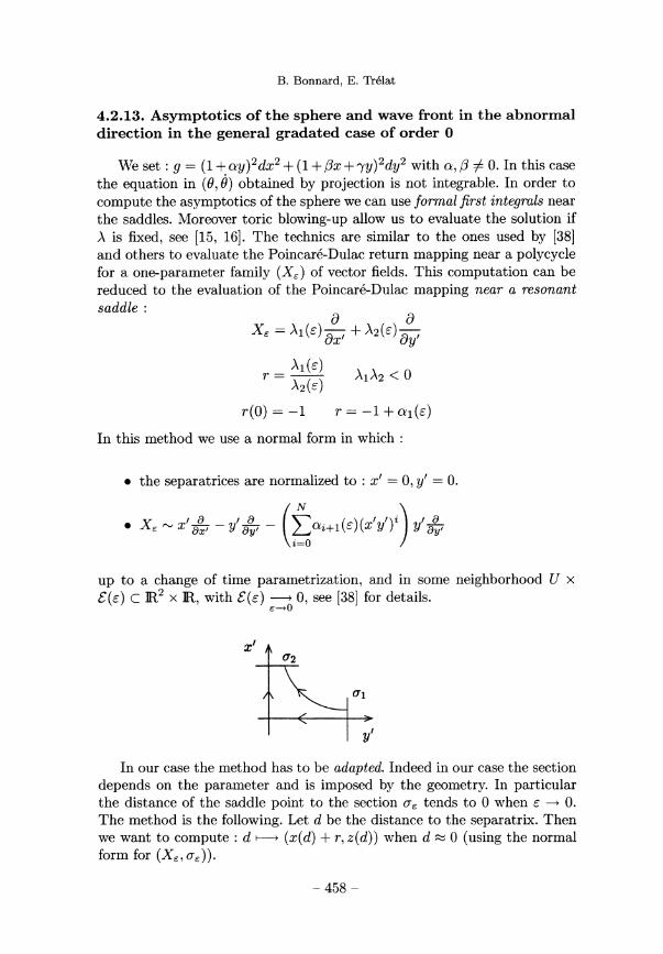
4.2.13. Asymptotics of the sphere and wave front in the abnormaldirection in the general gradated case of order 0

We set : g = with c~, ,~ ~ 0. In this casethe equation in (0, 8) obtained by projection is not integrable. In order tocompute the asymptotics of the sphere we can use formal first integrals nearthe saddles. Moreover toric blowing-up allow us to evaluate the solution ifA is fixed, see [15, 16]. The technics are similar to the ones used by [38]and others to evaluate the Poincaré-Dulac return mapping near a polycyclefor a one-parameter family (Xc) of vector fields. This computation can bereduced to the evaluation of the Poincaré-Dulac mapping near a resonantsaddle : :

_ _

In this method we use a normal form in which :

. the separatrices are normalized to : x’ = 0, y’ = 0.

up to a change of time parametrization, and in some neighborhood U x£(£) c IR2 x R, with ~(~) - 0, see [38] for details.

c-o

In our case the method has to be adapted. Indeed in our case the sectiondepends on the parameter and is imposed by the geometry. In particularthe distance of the saddle point to the section cr~ tends to 0 when 6* -~ 0.The method is the following. Let d be the distance to the separatrix. Thenwe want to compute : d ~---~ (x(d) + r, z(d)) when d x5 0 (using the normalform for ( X~ , ~~ ) ) .

This computation generalizes the computation in the conservative casewhere d is the distance to the root of multiplicity two of the potential.

The algorithm to evaluate step by step this application is to considerthe k-jet of (Xc, ac). It is not clear a priori that the k-jet is sufficient tocompute the first k terms in the expansion. However we shall prove that the1-jet is sufficient to compute the first term in the expansion. It gives us thecontact of the branch D1 with the abnormal direction.

PROPOSITION 4.16. - Let us suppose a = (1 ~ cxy)2, c = with a > 0. Let X = 2 T , Z = . Then near X = 0 the graph of the branchD1 is the following : :

Remark 4.6. - Observe that in the fiat case, the abnormal geodesic isnot strict and the contact is of order 1 (see prop 4.10).

Proof. - The differential system is :

Reparametrizing with: ds = ~~1+ay~~i+~x+~,y~ dt, we obtain:

Hence the equation governing 8 is :

The eigenvalues of the linearized system are solutions of : /~ 2014 -y=/~ 2014 (1 2014~)=0,hence=~=l+~+0~) , ~=-l+~+0(~).Let u == tti + = + 2u2. We get :

and after integration :

where A and B are constants to determine.

The section is y = 0, hence : v = ~ cos u + -~ sin u = ~ + ~u +o (-~- ) Let sf be the parameter corresponding to the final time t = r, i.e. :y(o) - y(sf) - 0. Putting these conditions in the previous equations weobtain :

Hence :

To get ?/, just note that : y = -1 03BB d03B8 ds + 03B1 03BB cos 03B8 - 03B2 03BB sin 03B8, hence :

Then we have to compute x, which amounts to integrating equation (39).We get :

The computation of z is then similar and we obtain :

It remains to estimate From the equation : £ == 2014(1 + +

~.r + uv) we get :

Remark 4.7. Another way to compute this expansion is to use thetheory developed in [42], which states that the so-called L°°-sector has acontact of order 2 with the abnormal direction, and moreover gives an ex-plicit formula to estimate the contact.

The previous method cannot be applied to study the contact of branchesCi and D2 with the abnormal direction, because in the phase plane ofthe pendulum these branches correspond to a global computation of returnmapping, and thus the calculations cannot be localized near a. saddle as

previously. Anyway inspecting carefully the system leads to the following :LEMMA 4.17. - In the general gradated case of order 0 the contact of

branches Cl and D2 with the abnormal direction is :

Note that contacts are still in the polynomial category.

Proof. 2014 We have : ~/ = hence = O(r). On the other part : ~~ =and thus : : x = u(1-I-O(r)). In the same way : z = u.~(1-~-()(r)).

Then the result in the flat case leads easily to the conclusion. r

D

Remark 4.8. From our previous study we can assert that minimizingcontrols steering 0 to points of Ci (resp. D2) are close to the abnormalreference control in L2-topology, but not in L~-topology. It is a (rucialdifference with the branch Dl.

Concerning the transcendance of this branch D1, the followiy fact proved in [43] :

PROPOSITION 4.18. - In the general gradated case of order 0, if a ~ 0then the branch D1 is C°° and is not subanalytic at x = -r, z = 0.

COROLLARY 4.19. - In the general gradated case of order 0, if the ab-normal minimizer is strict then the SR spheres with small radii are notsubanalytic.

Proof. Let A = (-r, 0, 0) denote the end-point of the abnormal trajec-tory. We shall prove that D1 is not subanalytic at A. The method is thefollowing. First of all the Maximum Principle gives a parametrization ofminimizing trajectories steering 0 to points of D1. Then we prove that theset of Lagrange multipliers associated to these points (i.e. end-points of thecorresponding adjoint vectors) is not subanalytic. Finally we conclude us-ing the fact that, roughly speaking, these vectors coincide with the gradientof the sub-Riemannian distance (where it is well-defined). These facts aresummarized in the following :

LEMMA 4.20. - To each point q of D1 is associated a control u. and

we denote by an associated Lagrange multiplier. Then we set :

where ~x (resp. ~z) is the projection on the axis x (resp. on the axis z)of the vector ~. If the set ,C is not subanalytic then the curve D1 is not

subanalytic.

Proof of the Lemma. Let be a parametrization of the curveD1 such that q(0) = A. For each T let uT be a control such that E(uT) -q(T), and let be an associated Lagrange multiplier, i.e. :

Then : - ~ ~

Moreover for each T the point q(T) belongs to the sphere S(0, r), hence= r, and thus : = 0. Therefore in the plane (y = 0) the

vectors of the set £ are unitary normal vectors to the curve Di. Then theconclusion is immediate. D

With notations of Proof of Proposition 4.16, we are now lead to studya family of vector fields (Xc) depending on the parameter £ = ~, in theneighborhood of a saddle point u = v = 0. For the section E correspondingto y = 0 we estimate the return time, i.e. the time needed to a trajectorystarting from £ to reach again £ ; then we claim that this time is t = r.This gives us a relation between O(r) and A, thus between and pz(r).

Then one has to show that this relation is not subanalytic. We proceed inthe following way. First of all recall that

We need a result which is independant of the parameter £ = -~=. So it is

no use trying to write an analytic normal form, since the saddle may beresonant. On the other hand C~ normal forms (see [38]) are not enoughbecause flat terms that we aim to exhibit disappear up to a Howevernear the saddle separatrices of Xc are analytic in u, v, E, and actually thereexists an analytic change of coordinates (u1, v1) - An(u, v) (in the sequelAn(.) denotes an analytic germ at 0) such that in these new coordinatesseparatrices are ui = 0, vi = 0, and the system is :

where ~cl ( ~ ), ~c2 ( ~ ) are the eigenvalues of the saddle ; in particular :2( 1 03BB) = -1+03B2 203BB+O(1 03BB). Moreover vve have : u = 1 ), v = ul-

vi + o( -£ ) , therefore the section is £ . vi = ui + -L + o( 1 03BB ) Let s j denotevl + o( 1 03BB ), therefore the section is 03A3 . vl = ul + 03B1 03BB -I- o( 1 03BB ) . Let s f denotethe parameter corresponding to the return time, i.e. {s f ), vl (s f )) E 03A3.We have : v1 (o) _ ~ ~-- o( ~ ) . Then :

On the other part : ~ = ~(l + + ~) = ~e-~’ + O(~).Hence we get:

And thus : ~ = -B/T~~+0(~). Putting into (45) we obtain finally:

In particular vl (sf) is not an analytic function in ~ .We know that v1 (s f) - An{u(s f), v(s f)) ~ u(sf)-v(sf) 2

. Moreover, onthe section ~, we have : v(sf) - - a cos u(sf) + ’~ sin u(sf). . Hence : °

v1{s f) = An(u(s f), 1 ) = u~2’t~ +~ ~ ~ From the Implicit Function Theoremin the analytic class we get : u(s f) ) - An(v1 (s f), 1 03BB). Therefore u ( s f ) is

not an analytic function in ~ . So the set £ is not subanalytic, which endsthe proof. D

Unfortunately we have no general result similar to Corollary 4.15. Wethink that the log-exp category is not wide enough in the non integrablecase. Indeed due to the dissipation phenomenon observed in the pendulumrepresentation if (3 ~ 0 we cannot expect to keep the analytic propertiesrequired in the definition of log-exp functions. Moreover in the phase planeof the pendulum, the foliation is not a priori integrable in the analyticcategory for any value of the parameter. We can observe that if we fix A to1 and evaluate the Poincaré-Dulac mapping, it is pfaffian if and only if Xc(A = 1) is CW-integrable (see [34, 35]).

Hence we conjecture :

CONJECTURE 4.21. - If (3 1= 0 then SR Martinet spheres are not log-exp, even not pfaffian.

Hence we should try to extend the log-exp category to a wider category inwhich analyticity would be replaced with some asymptotic properties. Thatis why we should be interested in Il Yashenko’s class of functions (see [22]).Indeed several years ago the Dulac’s problem of finiteness of limit cycles wassolved independantly by Ecalle and Il’Yashenko ; in his proof, Il’Yashenkointroduces a very wide class of non-oscillating functions to describe Poincaréreturn mappings. Actually he needs to expand real germs of functions intoterms having not only the order of x~" but also into flat terms. His categoryis contructed by recurrence as follows. Let M0 be a class of functions thatcan be expanded in an unique way into an ordinary Dulac’s series, i.e. seriesof the form :

where c > 0, the Pi’s are polynomial and (vi) is an increasing sequenceof positive numbers going to infinity. Wo only sketch the first step of therecurrence. By definition germs of the class can be expanded in seriescontaining flat exponential terms coefficients belong to Mo. For in-stance a super-accurate series of some germ f may be of the form :

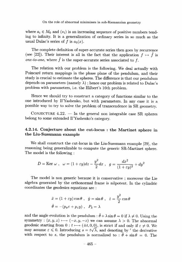
where ai E Mo and (vi) is an increasing sequence of positive numbers tend-ing to infinity. It is a generalization of ordinary series in so much as theusual Dulac’s series of f is ao(x). .

The complete definition of super-accurate series then goes by recurrence(see [22]). Their interest is all in the fact that the application f H / isone-to-one, where f is the super-accurate series associated to f .

The relation with our problem is the following. We deal actually withPoincare return mappings in the phase plane of the pendulum, and theirstudy is crucial to estimate the spheres. The difference is that our pendulumdepends on parameters (namely A) ; hence our problem is related to Dulac’sproblem with parameters, i.e. the Hilbert’s 16th problem.

Hence we should try to construct a category of functions similar to theone introduced by Il’Yashenko, but with parameters. In any case it is a

possible way to try to solve the problem of transcendence in SR geometry.

CONJECTURE 4.22. In the general non integrable case SR spheresbelong to some extended Il’Yashenko’s category.

4.2.14. Conjecture about the cut-locus : the Martinet sphere inthe Liu-Sussmann example

We shall construct the cut-locus in the Liu-Sussmann example [29], thereasoning being generalizable to compute the generic SR-Martinet sphere.The model is the following :

The model is non generic because it is conservative ; moreover the Liealgebra generated by the orthonormal frame is nilpotent. In the cylindriccoordinates the geodesics equations are :

and the angle evolution is the pendulum : 8 + A sin 03B8 = 0 0. Using thesymmetry : (x, y, z) ~--~ (-x, y, -z) we can assume ~ > 0. The abnormalgeodesic starting from 0 : t f--~ (~t, 0, 0), is strict if and only 0. Wemay assume ~ 0. Introducing s = and denoting by ’ the derivativewith respect to s, the pendulum is normalized to : + sin 03B8 = 0. The

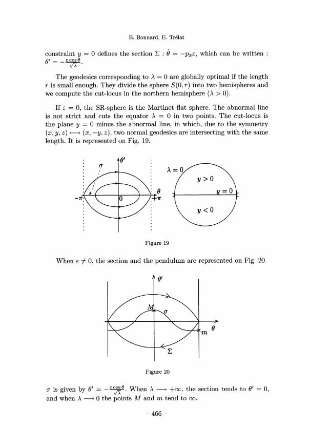
constraint y = 0 defines the section 03A3 : = which can be written :03B8’ = -~ cos 03B8 03BB.

The geodesics corresponding to A = 0 are globally optimal if the lengthr is small enough. They divide the sphere S’(o, r) into two hemispheres andwe compute the cut-locus in the northern hemisphere (A > 0).

If ~ = 0, the SR-sphere is the Martinet flat sphere. The abnormal lineis not strict and cuts the equator A = 0 in two points. The cut-locus is

the plane y = 0 minus the abnormal line, in which, due to the symmetry(x, y, z) ’2014~ (x, -y, z), two normal geodesics are intersecting with the samelength. It is represented on Fig. 19.

Figure 19

When ~ 7~ 0, the section and the pendulum are represented on Fig. 20.

Figure 20

a is given by 8’ - - ~ ~~e . when A -~ + 00, the section tends to 0’ = 0,and when A --~ 0 the points 1V1 and m tend to oo.

We can easily construct the cut-locus on the small sphere using thefollowing conjectures :

. Only the geodesics where the section a is in the configuration ofFig. 20 have cut-points (this is justified by the fact that when A = 0the geodesics are globally optimal if the length is small enough).

. A separatrix has no cut-point.

The trace of the sphere with the Martinet plane has been computed in[10]. An important property is that the rotating trajectories of the pendu-lum near the separatrix have a cut-point located in the plane y = 0, corre-sponding to its second intersection with y = 0. We represent on Fig. 21 theconstruction of the cut-locus.

Figure 21

The cut-locus has two branches Lc and LD corresponding respectively tooscillating and rotating trajectories. They ramify on the abnormal directionA which is not contained in the cut-locus. The extremities of the branchesLc and LD are conjugate points corresponding respectively to 0(0) = 7r

and 0(0) = 0. The branch Lc has only one intersection with y = 0 whichcorresponds approximatively to 0(0) = ~. . The cut-locus is not subanalyticat A but belongs to the log-exp category, and thus from [20] :

LEMMA 4.23. - The cut-locus is C~-stratifiable.

To generalize this analysis we must observe the following. The respectivepositions of the branches Ci, D2 are given in Section 4.2. Here the curve D2is above and hence the rotating trajectories are optimal up to the secondintersection. Also the integrability of the geodesic flow is not crucial and in

general the branch LD is not contained in the plane y = 0. We make thefollowing conjecture.

CONJECTURE 4.24. 1. In the Martinet case the cut-locus is C1-stratifiable.

2. In the generic case the cut-locus has two branches in the northernhemisphere ramifying at the end-point of the abnormal direction.

5. Some extensions of Martinet SR geometryand microlocal analysis of the singularity of the SR spherein the abnormal direction

5.1. Non properness and Tangency Theorem

This analysis is based on the sub-Riemannian Martinet case, where itwas shown in the previous Section that the exponential mapping is not

proper and that in the generic case the sphere is tangent to the abnormaldirection. This fact is actually general and we have the following results(see [40]).

Consider a smooth sub-Riemannian structure (1~~, 0, g) where M is aRiemannian n-dimensional manifold, n > 3, A is a rank m distribution onM, , and g is a metric on A. Let qo E ; our point of view is local andwe can assume that M = JRn and qo = 0. Suppose there exists a strict

(in the sense of definition 3.2) abnormal trajectory r passing through 0.Up to reparametrizing we can assume that A = Span ~Fl , ... , where

the system of Fi’s is g-orthonormal. Then the sub-Riemannian problem isequivalent to the time-optimal problem for the system :

where the controls satisfy the constraint ~~ 1 uf 1. Suppose further that~y is associated to an unique strictly abnormal control. Then : :

THEOREM 5.1. . - The exponential mapping is not proper near ~y.

Proof. - Set A = ~y(r), r > 0. Let (An) be a sequence of end-points ofminimizing normal geodesics qn converging to A. To each geodesic qn is

associated a control un and an adjoint vector (pn, p° ). As qn is normal wemay suppose that p° - - 2 . Let ~n the end-point of the adjoint vectorpn. Then if E denotes the end-point mapping and C is the cost (here the

cost is quadratic in the control), we have the following Lagrange multiplierequality :

If the sequence ~n were bounded then up to a subsequence it would convergeto some ’Ø E Now since the Un are minimizing the sequence (un) is

bounded in L2, hence up to a subsequence it converges weakly to someu E L2. Using the regularity properties of the end-point mapping (see [40]),we can pass through the limit in the previous equality and we get :

and on the other part : A = E(u). It is not difficult to see that u hasto be minimizing, and then we get a contradiction with the fact that r isstrict. n

Remark 5.1. - Conversely if the exponential mapping is not properthen actually there exists an abnormal minimizer. This shows the interac-tion between abnormal and normal minimizers. In a sense normal extremals

recognize abnormal extremals. This phenomenon of non-properness is char-acteristic for abnormality.

This non-properness is actually responsible for a phenomenon of tan-gency described in the following Theorem (see [42] for a more general state-ment): :

THEOREM 5.2. . - Consider the SR system (/ 6) and suppose there existsa minimizing geodesic ~y associated to an unique strictly abnormal controlu. Let A G S(o, r) be the end-point Assume is a C1 curveon S(o, r) such that lim = A. Then : lim ~’(T) E Im dE(u).

T-~O T~O

In particular if ,S’(o, r) is Cl-stratifiable near A then the strata of ,S’(o, r)are tangent at A to the hyperplane Im dE(u) (see Fig. 22). Moreover if Bis a C1-branch of the cut-locus ramifying at A then B is tangent at A tothis hyperplane.

Proof. - For each T the point is the end-point of a minimizing geodesic,and we denote by (pT, p° ) (resp. uT) an associated adjoint vector (resp. anassociated control). Let (~T, ~°) be the end-point of this adjoint vector. Wemay suppose that it is unitary in Rn x R. We have :

Figure 22. - Tangency phenomenon

Using the same reasoning as in the Proof of Theorem 5.1 we get that ~ ~ ~° ~ ~ -~0 as T --~ 0. To conclude it suffices to show that is normal to the curve

o-(T) Indeed the previous equality implies :

But C(ur) is constant (equal to r) and E(ur) = a(ur), and thus :

which ends the proof. D

5.2. The tangential case

5.2.1. Preliminaries

In this Subsection we shall make a brief analysis of the so-called tan-gential case. According to Section 2.2.2 the distribution D = Ker w can bereduced [45] to one of the normal forms :

where ~ _ ~ 1. The parameter 6; is a deformation parameter whose in-troduction will be justified later.

A general metric g is then defined by : : a(q)dx2 + 2b(q)dxdz + c(q)dz2where a, b, c can be taken as constant in the nilpotent approximation oforder -1. Our study is far to be complete and we shall describe briefly thecase g = dx2 + dz2.

The general case of order -1 depends on a parameter A and correspondsto a 6-dimensional nilpotent Lie algebra. It contains both elliptic and hy-perbolic cases. It is the Lie algebra generated by Fl, F2 with the followingLie brackets relations :

and all other Lie brackets are 0.

Introducing Pi = p, Fi > the geodesic equations are given by :

and P6 is a Casimir first integral. The value A = 0 represents the bifurcationbetween the two cases.

5.2.2. Abnormal geodesics

Elliptic case The abnormal geodesics are contained in the Martinet sur-face :

and are solutions of the equations :

From [45], the singularity x = z = 0 is a weak focus and a spiral passingthrough 0 is with infinite length. Since any minimizer is smooth no pieceof abnormal geodesic is a minimizer when computing the distance to 0.

Using the general result of [I], the sphere of small radius is the image bythe exponential mapping of a compact set and it is subanalytic. This is alsoclearly shown by numerical simulations and the sphere is represented onFig. 23.

Figure 23. - Elliptic case

By taking E = 0, the Martinet surface becomes : x2 + z2 + 3mx2 z2 = 0and reduces near 0 to : x - z - 0. Hence the spiral disappears. Sincethe weight of x, z is one and the weight of y is four, it corresponds to thenilpotent approximation of order -1 where m is 0.

Hyperbolic case The Martinet surface is given by the equation :

and the abnormal geodesics are solutions of :

and the singularity at x = z = 0 is a saddle point. The two lines x = 0 andz = 0 are optimal for the metric dx’ + dz2. Hence they play a role whencomputing the distance to 0. Numerical simulations show that the sphereis not the image of a compact set. This can be seen on Fig. 24 because thesphere cannot be numerically represented in the abnormal direction (there

is a hole). It is similar to the situation encountered in the Martinet case.The sphere is pinched in both abnormal directions.

The nilpotent approximation of order -1 is obtained by taking E = 0and m = 0. The Martinet surface becomes : xz = 0 and the two lines x = 0and z = 0 remain abnormal geodesics.

Figure 24. - Hyperbolic case

5.2.3. Normal geodesics

Elliptic case We take the frame :

and we introduce : Pi = p, Fi (q) >. The geodesics equations are :

and they can be truncated at order -1 by making 6’ = m = 0. In this caseP3 is a first integral and we can set : P3 = A. Moreover if we introduce :P1 = sin 03B8, P2 = cos 03B8, the equations become :

They can be projected onto the space (x, y, 0) and the foliation is definedby :

It is not Liouville-integrable but the equations can be integrated byquadratures, see [36]. Using polar coordinates : x = r cos z = r sin it

becomes :

The important property is the following : :

LEMMA 5.3. - The sign of 8 is constant and reparametrizing the tion can be rewritten : 03B8 = 1 as in the contact case.

Numerical simulationsThe geodesics equations can be integrated numerically. The projec-

tions in the plane (x, z) of the geodesics starting from 0 are flowers withthree petals (they are circles in the Heisenberg case), see Fig. 25.

Figure 25

Hyperbolic case We take the frame :

and we introduce : Pi = p, Fi (q) >. The geodesics equations are :

and they can be truncated at order -1 by making E = m = 0. In this caseP3 is a first integral and we can set : P3 - A. Moreover if we introduce :Pi = sin0, P2 = cos 03B8, the equations become :

They can be projected onto the space (x, z, B). .

Numerical simulationsThe projected equations : : x = sin 0, ,z = cos 0, B = -2xz03BB can be

integrated numerically and the solutions compared with the pendulum :x = sin 0, z = cos 0, 8 = -~x, see Fig. 26. The behaviour is quite chaoticand 0 exhibits oscillating and dissipative phenomena. Also it shows in theplane (x, z) a coupling effect between the two abnormal directions.

The SR sphere in the tangential hyperbolic sphere is represented onFig. 27.

Figure 26

5.2.4. Conclusion -

.

The elliptic situation is similar to the contact case. The analysis of thehyperbolic case is intricate. A tool to study the sphere is to introduce as

Figure 27. - Tangential hyperbolic sphere

in the Martinet case a return mapping by taking the intersections of thegeodesics with one of the planes : x = 0 or z = 0. The non properness ofthis application can be checked numerically.

5.3. The Engel case and left-invariant SR geometry on nilpotentLie groups

If q = (x, y, z, w), we consider the system in R~ :

We have the following relations : F3 = ~Fl , F~~ = a -~-y ~ , F4 = ~~Fl, F2~, F2~ _~ ~03C9 and [[Fi, F2] , F1] = 0. Moreover all Lie brackets with length greater than4 are equal to zero. Set :

and define the following representation : p(Fi) = L1, p(F2) - L2 whichallows to identify the previous system in IR4 to the left-invariant system R =

(ulLi + u2L2)R on the Engel group Ge, here represented by the nilpotentmatrices :

The weight of x, y is one, the weight of z is two, and the weight of w isthree. For any sub-Riemannian metric on Ge, the approximation of order- 1 is the flat metric g = dx2 + dy2. Any sub-Riemannian Martinet metriccan be written g = adx2 + cdy2 and can be lifted on Ge . .

5.3.1. Paramatrization of geodesics in the flat case

Non trivial abnormal extremals are solutions of :

Set p = py, pz, We get :

This implies 0 and thus u2 = 0. The abnormal fiow is given by :

where |u1| ( = 1 if the parameter is the length.

To compute normal extremals, we set Pi == p, Fi (q) >, i = 1 , 2, 3, 4 and

Parametrizing by the length ~I~ - 2 , we may set : P1 - cos B, P2 - and we get : = -P3, = -P2P4. Denote P4 - 03BB, then this isequivalent to the pendulum equation :

Let L denote the abnormal line starting from 0 : t ’2014~ (~t, 0, 0, 0). It isnot strict and projects onto 8 =

In order to obtain an uniform representation of normal geodesics, weshall use the Weierstrass elliptic function P. Indeed the system admits three

integrals : : Pi + P2 = 1, and two Casimir functions : -2P1P4 + P3 == Cet P4 - A. Using Pl = P2P3 we get : Pl = -CPi - 3APi + A, which isequivalent, with 0 and a ~ 0, to the equation : -2~(Pi +~ P1 - Pi + D). Let P(u) denote the Weierstrass elliptic function (cf [26])solution of :

where the complex numbers ei satisfy ei + e2 + e3 = 0. Set g2 = -4(e2e3 +e3e1 + e1e2) and g3 = 4e1e2e3 ; then : ~’(u) = 4~3(u) - - g3. Thefunction P(u) can be expanded at 0 in the following way :

Hence the solution Pi can be written : aP(u) + b. Then we can computeP2 and P3 using the integrals, and x, y, z, w can be computed by quadra-tures. We find again oscillating and rotating solutions of the pendulum usingJacobi elliptic functions given by the formulas :

5.3.2. Heisenberg and Martinet flat cases deduced from the Engelcase. Blowing-up in lines

Note that the two vector fields a~ and tw commute with Fi and F2. TheEngel case contains the flat contact case and the flat Martinet case whichare given by the following operations :

. Setting pz = 0, we obtain the geodesics of the Heisenberg case.

. Setting pw = 0, we obtain the geodesics of the Martinet flat case.

The interpretation is the following.LEMMA 5.4. - We obtain the Martinet flat case (resp. Heisenberg) by

minimizing the SR distance to the line (Oz) (resp. (Ow)).

Indeed the condition pz = 0 (resp. pw = 0) corresponds to the transver-sality condition. It may be observed that, since the SR distance to a line ismore regular than to a point, the SR distance in the Engel case has at leastall-singularities of the Heisenberg and Martinet flat cases.

Another way to get the Martinet flat case is to use the following generalfact from [7] :

LEMMA 5.5. - The Martinet flat case is isometric to where H is the following sub-group of Ge F2~ / t E .

The Engel case can be imbedded in any dimension, for more detailsabout left-invariant SR-geometry on nilpotent Lie groups see [39].

In the Martinet fiat case, using the uniform parametrization of thegeodesics by elliptic functions, the sphere is evaluated in any direction.

Next we give a description of the SR sphere in an abnormal directionwhen the flag associated to the distribution D satisfies D3 ~ D2, see Sec-tion 3.4.

5.4. Microlocal analysis of the singularity of the SR sphere in theabnormal direction

The aim of this Section is to stratify the singularity of the SR sphere inthe abnormal direction. We use symplectic geometry. This leads to a strat-ification of the solutions of the Hamilton-Jacobi-Bellman equation viewedin the cotangent bundle.

5.4.1. Lagrangian manifolds and generating mapping

DEFINITION 5.1. - Let (M, w) be a smooth symplectic manifold andL C M be a smooth regular submanifold. We say that L is isotropic if therestriction of w to T L is equal to zero, and if dim L = ~dim ~.T then L iscalled Lagrangian.

’

The following result is crucial, see [32]. .

PROPOSITION 5.6. - Let (M, w) be a 2n-dimensional manifold and L cM be a Lagrangian submanifold. Then there exists Darboux local coordinates(q, p) and a smooth function S(qI, pI) where I = ~l, ... I = ~m +l, ... , n~ is a partition of ~l, ... , n~ such that L is given locally by theequations : :

~ ~ - ~

DEFINITION 5.2. - The mapping S which represents locally L is calledthe generating mapping of L.

DEFINITION 5.3. - Let L be a Lagrangian manifold and n the standardprojection (q, p) H q from TM onto The caustic is the projection on Mof the singularities of (L, n).

5.4.2. Lagrangian manifolds and SR normal case

Consider the SR problem :

where the length of q is :

We use the notations of Section 3.2. Let Pi = p, Fi (q) >, i = 1, 2, theHamiltonian associated to normal geodesics is given by Hn = + P2 ) .

Let t - [0, T] be a reference one-to-one normal geodesic. Weassume the following :

Hypothesis : We assume that the reference geodesic is strict,i.e. there exists an unique lifting [1] of 03B3 in the projectivebundle .

Notations

. is the exponential mapping. If the geodesics are parametrizedby arc-length Hn = 2, it is defined by t ~ II(q{t)) where t H q(t) isa solution of fin starting from q(0) at time t = 0.

. Lt = exp where exp tHn is the local one-parameter

group associated to .

The length of a curve does not depend on the parametrization and theoptimal control problem is parametric. This induces a symmetry which hasto be taken into account when writing Hamilton-Jacobi equation in thenormal case. Indeed we have : :

LEMMA 5.7. - The solutions of Hn satisfy the relation : :

The following results are standard :

PROPOSITION 5.8. 1. . Lo = is a linear Lagrangian manifold,and for each t > 0, Lt is a Lagrangian manifold.

2. The time tc is conjugate along 03B3 if and only if the projection II :Lt~ -~ M is singular at .

3. Assume that geodesics are parametrized by arc-length t; and let

where T tic (first conjugate time along ~y. Then ~ = is acentral field along ~y. .

Remark 5. 2.. The caustic of Lt is the set of conjugate points whichcan be analyzed using Lagrangian singularities.

. We represent locally W by an Hamilton-Jacobi or wave function de-fined as follows. We integrate the normal flow starting from -y(o) andparametrized by arc-length : Pf -I- P2 = 1. By setting = cos 0,this gives us the family of geodesics :

and p is eliminated by solving the equation E(p) = q near usingthe Implicit Function Theorem. Beyond the computations need thePreparation Theorem and Legendrian singularity theory.

Next we describe the tangent space to the Lagrangian manifold.

DEFINITION 5.4. - We denote by (Vn ) the variational equation :

along the reference trajectory t ~--~ %y(t). This Hamiltonian linear equationis called Jacobi equation. A Jacobi field J(t) _ (~q{t), ~p(t)) is a nontrivialsolution of (47). It is called vertical if bq(o) = 0.

PROPOSITION 5.9. l. Let Lt = exp . Then the space ofvertical Jacobi fields is the tangent space to Lt for t > 0.

2. Assume we are in the analytic category. Let J(.) be a vertical Jacobifield and let ~ H be an analytic curve such that - J(o) .If Y is an analytic vector field on T * M such that Y {=y (o) ) - a (o) ;then t H J(t) is given for t small by the Baker-Campbell-Hausdorffformula :

A consequence of Lemma 5.7 is :

LEMMA 5.10. - Let =y(0) = (qo, po) and consider the curve -

(qo, po + . Then it is a vertical curve, and if Jl is the associated Jacobi

field then II( Jl (t)) = .

5.4.3. Isotropic manifolds and SR abnormal case

Consider the system q = ul Fl (q) + u2F2 (q) According to Section 3, theabnormal geodesics are solutions of the equations :

where Ha = u1P1 + u2P2 They are contained in :

and the abnormal controls are computed using :

Assumptions. Let t ’2014~ [ -T, T] be a. one-to-one abnormal referencegeodesic. One may assume that it corresponds to the control u2 = 0. Wesuppose that the following conditions are satisfied along q for the couple(Fl, F2), see Section 2.5.

(HI) The first order Pontryagin’s cone K(t) = Span / k E :IN}has codimension one and is generated by ~F2, ... .

(H2) If n > 3, for each t, Fl(-y(t)) ~ Span / k = 0... n - 3~.

(H3) ~P2~ ~’2~~ ~ 0 along ~y.

Notations

. Under the previous assumptions r admits an unique lifting [i] =in P(T*M). . One may identify locally AI to a neighborhood

U of q(0) = 0 in Let V be a neighborhood of p03B3 in P(To U). Wecan choose V small enough such that all abnormal geodesics startingfrom ~0~ x V satisfy the assumptions (Hi - H3). We denote by Erthe sector of U covered by abnormal geodesics with length ~ r andstarting from ~0~ x V. This defines a mapping denoted Exp. Theconstruction is represented on Fig. 28.

. On Q = T*MB(~~Pl, P2~, P2~ = 0) let Ha be the Hamiltonian Ha =

Pi + icP2 where û = -{{P1,P2},P1} {{P1,P2},P2}, and let exp di a be the one-parameter local group. We denote by Lf (resp. If) the image of

(resp. n (Pl = P2 = {P1, P2} _ 0)).

LEMMA 5.11. - On Q; Lf is a Lagrangian submanifold and If is an

isotropic submanifold.

Figure 28

5.4.4. The smooth abnormal sector of the SR sphere

LEMMA 5.12. - Consider the SR problem where ~y is an abnormal ref-erence trajectory and assume (Hl - H3). . It can be identified to a trajectoryoffi where the system (Fl, F2) is orthonormal. Then the abnormal geodesicis strict, and there exists r > 0 such that if the length of ~~ is less than rthen ~y is a global minimizer.

Proof. - Under assumption (Hi) the first order Pontryagin’s cone along~y has codimension one, and from (H3) ~y is not a normal geodesic. Theoptimality assertion follows from [6], see also [29]. 0

Hence the end-point of 03B3 belongs to the sphere. Moreover r can beestimated and the estimate is uniform for each abnormal geodesic C1-closeto q. Therefore we have :

PROPOSITION 5.13. - For r small enough ~r is a sector of the SR ballhomeomorphic to C U -C, where C is a positive cone of dimension n - 3 ifn > 4 and 1 if n = 3. Its intersection with the sphere consists of two (C°°or CW ) surfaces of dimension n - 4 if n > 4 and reduced to two points ifn = 3.

5.4.5. Gluing both normal and abnormal parts

The tangent space to the sphere near the abnormal directions is describedby the results of Section 5.1, namely Theorem 5.2.

Let A be the end-point of the abnormal trajectory and let K(r) be thefirst order Pontryagin’s cone evaluated at A, r small enough. Let s - -

be a C1 curve on the sphere S’(o, r), a(0) = ~4, ~ ~ 0. Assume the following :

1. a(E) C ,S’(o, r)~~r 0.

2. cx (~) n L = 0, where L is the cut-locus for geodesics starting from 0.

Then the tangent space to the sphere evaluated at a(e) tends to K(r) whenE - 0 (see Fig. 29).

Figure 29

5.4.6. Lagrangian splitting and the Martinet sector

DEFINITION 5.5. - We call Martinet sector of the Martinet sphere thetrace of the ball B(0, r) with the Martinet plane identified to y = 0.

A precise description is obtained if we use the pendulum representationof Section 4, where the metric is truncated to order 0 : g = (1 + +

(1 + ,~x + The abnormal geodesic is strict if and only if a ~ 0. Thependulum equation is :

where £ = 2014= is a parameter. Cutting by y = 0 induces a one-parametersection :

The trace of the sphere with the Martinet plane near the end-point A =

(-r, 0, 0) of the abnormal direction is described in Section 4. We take thefirst and second intersections of the pendulum trajectories with ,S’, see

Fig. 30.

In the conservative case, the curves Di, D2 correspond to oscillatingtrajectories of the pendulum, and the curve Ci corresponds to rotating tra-jectories.

Figure 30. - (a ~ 0)

Only one of the curves C1, D2 belongs to the sphere (this is D2 on thefigure) and their respective positions depend on the Gauss curvature of therestriction of the metric g to the plane (x, y) .

Contacts are the following.

PROPOSITION 5.14. - Let Z = ~ and X = rr . Then :

Cl, D2 : Z = (6 + + O(X3).

D1 : Z = - ~,~X2 + o(X2).

This allows to describe the Martinet sector in the ball.

PROPOSITION 5.15. - In the strict case a ~ 0 the Martinet hasthe following properties.

1. It is the image by the exponential mapping of a non compact subsetof the cylinder : : (B(o), ~), a -~ oo.

2. It is homeomorphic to a conic sector centered on the abnormal line.3. It is foliated by leaves D1, E1 in the spheres S(0,~), E r. u’h ll’jl glue

according to Fig. 31.

Figure 31

The Lagrangian splitting. In the pendulum representation, the trans-port of n {Hn = ~} by the normal flow has the following basicinterpretation, see Fig. 32.

Figure 32

The section splits into two parts 62 which represent the splitting ofthe fiber T,~(o) ~.l into two Lagrangian manifolds.

5.4.7. Microlocal invariants

The pendulum has two singular points F = (0,0) and S = (o, ~r). Thelocal analysis is as follows.

. Near F, the linearized system is a focus whose eigenvalues are :

and is a perturbation of the linearized pendulum 0" + 0 = 0 of theflat case.

. Near S, the linearized system is a saddle whose eigenvalues are :

where £ = ~ . It is a perturbation of the flat case == ~l which is

- resonant.

In order to compute the sector we use the spectrum band which is

stable by perturbation. When we compute the sphere we have to computean averaging. This is much more complex.

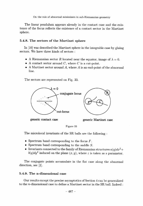
The linear pendulum appears already in the contact case and the exis-tence of the focus reflects the existence of a contact sector in the Martinet

sphere.

5.4.8. The sectors of the Martinet sphere

In [10] was described the Martinet sphere in the integrable case by gluingsectors. We have three kinds of sectors :

. A Riemannian sector R located near the equator, image of A = 0.

. A contact sector around C, where C is a cut-point.

. A Martinet sector around A, where A is an end-point of the abnormalline.

The sectors are represented on Fig. 33.

Figure 33

The microlocal invariants of the SR balls are the following :

. Spectrum band corresponding to the focus F.

. Spectrum band corresponding to the saddle S.

. Invariants connected to the family of Riemannian structures a(q)dx2+induced on the plane (x, ~), where z is taken as a parameter.

The conjugate points accumulate in the flat case along the abnormaldirection, see [2]. .

5.4.9. The n-dimensional case -

Our results except the precise asymptotics of Section 4 can be generalizedto the n-dimensional case to define a Martinet sector in the SR ball. Indeed :

. L2-compactness of SR minimizers (see [1]) allows to bound the num-ber of oscillations of Lagrangian manifolds. It appears in our studyby taking only the first and second return mapping to compute thesphere intersected with y = 0.

. From [41], using a normal form, we can cut the SR ball by a 2-dimensional plane to identify a Martinet sector which splits into twocurves : a curve Di obtained by using minimizing controls close to thereference abnormal control in L°°-topology ; a curve Ei obtained byusing controls close to the reference abnormal control in L2-topology,but not in L~-topology (see Fig. 34).

Figure 34

The picture explains well the consequence of the existence of abnor-mal minimizers in SR geometry. Contrarily to the classical case we cannotstraight the geodesic flow near the abnormal direction to form a central field.

6. Conclusion

Our analysis explains the role of abnormal geodesics in SR geometry. It isbased on the Martinet case. Using our gradated normal form of order 0, thegeodesics foliation is projected onto a one-dimensional foliation in a planewhich corresponds to a one-parameter family of pendulums. In this spacethe abnormal line projects on the singularities of the foliation. The compu-tation of the sphere in the abnormal direction is related to the computationof return mappings evaluated along tho separatrices of the pendulum. Wehave computed asymptotics, using techniques similar to the ones used inthe Hilbert’s 16th problem. The computations are complex, because it is asingular perturbation analysis. In these computations one needs to considergeodesics C1-close to the abnormal reference trajectory on the one part, andgeodesics which are C°-close, but not C1-close to the abnormal referencetrajectory on the other part. Our asymptotics are not complete in the lattercase and this requires further studies. Moreover the techniques have to be

adapted to analyze the general case when the geodesics equations are notprojectable. This leads to stability questions about our asymptotics.

The projection of the geodesics flow onto a planar foliation, valid at order0 in the Martinet case, is useful to compute asymptotics but is not crucialfrom the geometric point of view, and Martinet geometry is representativeof SR geometry with abnormal minimizers. The existence of such minimizersimplies hyperbolicity seen in the pendulum representation as the behaviorsof the geodesics near the separatrices. The general geometric framework toanalyze SR geometry is Lagrangian manifolds. Here hyperbolicity due tothe existence of abnormal directions is interpretated as a splitting of theLagrangian fiber when transported by the normal flow. To constructthe sphere in the abnormal direction we must glue together the projectionsof several manifolds in the cotangent space.

The link between the computations of asymptotics and Lagrangian ge-ometry is the Jacobi fields which allow to compute contacts for the returnmapping underlying our analysis. In general the evaluation of a return map-ping in the analysis of a differential equation interpretated as a transportproblem is original and source of further studies.

The question of the category of the SR Martinet sphere is still open.The Martinet sector is homeomorphic to a locally convex cone and we havegiven a qualitative description of its singularities. In the integrable casethe SR sphere is log-exp and this leads to a smooth stratification of thesphere. In general we conjecture that the sphere is not log-exp, belongs tosome extended Il’Yashenko’s category, and is still C1-stratifiable. It is an

important question connected to Hamilton-Jacobi equation which has manyapplications in physics (optics, quantum theory). For control theory, SRgeometry is part of optimal control. Moreover our study is related to thestabilization problem.

Bibliography

[1] AGRACHEV (A.). - Compactness for sub-Riemannian length minimizers and suban-alyticity, Rend. Semin. Mat. Torino, Vol. 56, 1999.

[2] AGRACHEV (A.), BONNARD (B.), CHYBA (M.), KUPKA (I.). - Sub-Riemannian spherein the Martinet flat case, ESAIM/COCV, Vol. 2, 377-448, 1997.

[3] AGRACHEV (A.), EL ALAOUI, GAUTHIER (J.P.). - Sub-Riemannian metrics on R3,Canadian Math. Cont. Proc., Vol. 25, 29-76, 1998.

[4] AGRACHEV (A.), EL ALAOUI, GAUTHIER (J.P.), KUPKA (I.). - Generic singularitiesof sub-Riemannian on IR,3, C.R.A.S., Paris, 377-384, 1996.

[5] AGRACHEV (A.), SARYCHEV (A.). - On abnormal extremals for Lagrange variationalproblems, J. Math. Systems, Estimation and Control, Vol. 8, No. 1, 1998, 87-118.

[6] AGRACHEV (A.), SARYCHEV (A.). - Strong minimality of abnormal geodesics for 2-distributions in SR-geometry, J. of Dynamical and Control Systems, Vol. 1, No. 2,139-176, 1995.

[7] BELLAÏCHE (A.), RISLER (J.J.) (Editors). - Sub-Riemannian geometry, Birkhäuser,1996, Progress in Mathematics, Vol. 144.

[8] BLISS (G.A.). - , Lectures on the calculus of variations, University of Chicago Press,Chicago, 1946.

[9] BONNARD (B.). - Feedback equivalence for nonlinear systems and the time optimalcontrol problem, SIAM J. on control and optimization, 29, 1300-1321, 1991.

[10] BONNARD (B.), CHYBA (M.). 2014 Méthodes géométriques et analytiques pour étudierl’application exponentielle, la sphère et le front d’onde en géométrie SR dans le casMartinet, ESAIM/COCV, Vol. 4, 245-334, 1999.

[11] BONNARD (B.), HEUTTE (H.). - La propriété de stricte anormalité est générique,Preprint Labo. de Topologie Dijon, 1995.

[12] BONNARD (B.), KUPKA (I.). - Théorie des singularités et optimalité des trajectoiressingulières dans le problème du temps minimal, Forum Math. 5, 111-159, 1991.

[13] BONNARD (B.), KUPKA (I.). - Generic properties of singular trajectories, Annales del’IHP, Analyse non linéaire, Vol. 14, No. 2, 167-186, 1997.

[14] BONNARD (B.), LAUNAY (G.), TRÉLAT (E.). - The transcendence we need to computethe sphere and wave front in Martinet SR-geometry, Contemporary Mathematicsand its Applications, Vol. 64, VINITI, Moscow, 1999, pp 82-117. English version inJournal of Mathematical Sciences (Kluwer), Vol. 103 (6), 2001, pp 688-708.

[15] BRUNO (A.D.). - Local methods in nonlinear differential equations, Springer Verlag,1989.

[16] CHAPERON (M.). - Géométrie différentielle et singularités des systèmes dynamiques,Astérisque 138-139, SMF, 1986.

[17] CHYBA (M.). 2014 Le cas Martinet en géométrie sous-Riemannienne, Thèse de

l’Université de Bourgogne, 1997.

[18] DAVIS (H.). 2014 Introduction to nonlinear differential and integral equations, Dover,1962.

[19] VAN DEN DRIES (L.), MACINTYRE (A.), MARKER (D.). 2014 The elementary theory ofrestricted analytic fields with exponentiation, Annals of Mathematics, 140, 183-205,1994.

[20] VAN DEN DRIES (L.), MILLER (C.). - Geometric categories and o-minimal structures,Duke Math. Journal, Vol. 84, No. 2, 1996.

[21] HEUTTE (H.). - Propriétés génériques des extrémales singulières dans le cas multi-entrée, Preprint Labo. de Topologie Dijon, 1995.

[22] IL’YASHENKO (Yu.S.). 2014 Finiteness theorems for limit cycles, Translations of Math-ematical Monographs, Vol. 94, 1991.

[23] KRENER (A.J.). - The higher order maximal principle and its applications to singu-lar extremals, SIAM J. on Control and Opt., Vol. 15, 256-293, 1977.

[24] KUPKA (I.). 2014 Abnormal extremals, Preprint, 1992.

[25] KUPKA (I.). 2014 Géométrie sous-Riemannienne, Séminaire Bourbaki, 1996.

[26] LAWDEN (D.F.). - , Elliptic functions and applications, Springer Verlag, 1980.

[27] LEE (E.B.), MARKUS (L.). - Foundations of optimal control theory, John Wiley, NewYork, 1967.

- 491 -

[28] LION (J.M.), ROLIN (J.P.). 2014 Théorèmes de préparation pour les fonctions

logarithmico-exponentielles, Annales de l’Institut Fourier, Tome 47, Fasc. 3, 859-884,1997.

[29] LIU (W.S.), SUSSMANN (H.J.). - Shortest paths for sub-Riemannian metrics of ranktwo distributions, Memoirs AMS, No. 564, Vol. 118, 1995.

[30] LOJASIEWICZ (S.), SUSSMANN (H.J.). - Some examples of reachable sets and optimalcost functions that fail to be subanalytic, SIAM J. on Control and Opt., Vol. 23, No.4, 584-598, 1985.

[31] LOVE (A.E.H.). - A treatise of the mathematica theory of elasticity, Dover, 1944.[32] MISCHENKO (A.S.) and al. - Lagrangian manifolds and the Maslov operator,

Springer Verlag, New York, 1980.

[33] MONTGOMERY (R.). - Abnormal minimizers, SIAM J. on Control and Opt., Vol. 32,No. 6, 1605-1620, 1997.

[34] MOURTADA (A.), MOUSSU (R.). - Applications de Dulac et applications pfaffiennes,Bulletin SMF, 125, 1-13, 1997.

[35] MOUSSU (R.), ROCHE (A.). - Théorie de Khovanski et problème de Dulac, Inv.

Math., 105, 431-441, 1991.

[36] PELLETIER (M.). - Communication personnelle.[37] PONTRIAGUINE (L.) et al. - Théorie mathématique des processus optimaux, Eds Mir,

Moscou, 1974.[38] ROUSSARIE (R.). - Bifurcations of planar vector fields and Hilbert’s 16th problem,

Birkhäuser, Berlin, 1998.

[39] SACHKOV (Y.L.). - Symmetries of flat rank two distributions and sub-Riemannianstructures, Preprint Labo. de Topologie Dijon, 1998.

[40] TRÉLAT (E.). 2014 Some properties of the value function and its level sets for affinecontrol systems with quadratic cost, Journal of Dynamical and Control Systems,Vol. 6, No. 4, Oct. 2000, 511-541.

[41] TRÉLAT (E.). - Etude asymptotique et transcendance de la fonction valeur en

contrôle optimal ; catégorie log-exp dans le cas sous-Riemannien de Martinet. PhdThesis, Université de Bourgogne, Dijon, 2000.

[42] TRÉLAT (E.). - Asymptotics of accessibility sets along an abnormal trajectory,ESAIM/COCV, Vol. 6, 387-414, 2001.

[43] TRÉLAT (E.). - Non subanalyticity of sub-Riemannian Martinet spheres, CRAS,t. 332, Série I, 527-532, 2001.

[44] ZELENKO (I.), ZHITOMIRSKI (M.). - Rigid paths of generic 2-distributions on 3-

manifolds, Duke Math. Journal, Vol. 79, No. 2, 281-307, 1995.

[45] ZHITOMIRSKI (M.). 2014 Typical singularities of differential 1-forms and pfaffian equa-tions, Trans. of Math. Monographs, Vol. 113, AMS, 1992.