on the rotation sets of homeomorphisms and flows on toriresumo estudamos os conjuntos de rota˘c~ao...
TRANSCRIPT

Universidade Federal da Bahia - UFBA
Instituto de Matematica e Estatıstica - IME
Programa de Pos-Graduacao em Matematica - PGMAT
Tese de Doutorado
On the rotation sets of homeomorphismsand flows on tori
Heides Lima de Santana
Salvador-Bahia
Dezembro de 2018

On the rotation sets of homeomorphismsand flows on tori
Heides Lima de Santana
Tese apresentada ao Colegiado do Programa de
Pos-Graduacao em Matematica UFBA/UFAL
como requisito parcial para obtencao do tıtulo
de Doutor em Matematica, aprovada em 17 de
Dezembro de 2018.
Orientador: Prof. Dr. Paulo Cesar Rodrigues
Pinto Varandas
Salvador-Bahia
Dezembro de 2018

Santana, Heides Lima.
On the rotation sets of homeomorphisms and flow on tori / Heides
Lima de Santana. – Salvador, 2018.
80 f. : il
Orientador: Prof. Dr. Paulo Cesar Rodrigues Pinto Varandas.
Tese (Doutorado - Matematica) – Universidade Federal da Bahia,
Instituto de Matematica, 2018.
1. Conjunto de rotacao. 2. Propriedade de colagem de orbita.3.
Dimensao media metrica. 4. Especificacao. 5. Homeomorfismo do toro.
I. Paulo Cesar Rodrigues Pinto Varandas. II. Tıtulo.

On the rotation sets of homeomorphisms and flowon tori
Heides Lima de Santana
Tese apresentada ao Colegiado do curso de
Pos-Graduacao em Matematica da Universidade
Federal da Bahia como requisito parcial para
obtencao do tıtulo de Doutor em Matematica,
aprovada em 17 de Dezembro de 2018.
Banca examinadora:
Prof. Dr. Paulo Cesar Rodrigues Pinto Varandas - UFBA
(Orientador)
Prof. Dr. Cristina Lizana Araneda - UFBA
Prof. Dr. Thiago Bomfim Sao Luiz Nunes - UFBA
Prof. Dr. Rodrigo Lambert - UFU
Prof. Dr. Wescley Bonomo - UFES

Ao meu pequeno Isaac Lima.

Agradecimentos
Agradeco primeiramente a Deus por me possibilitar chegar ate aqui.
Agradeco a todos os colegas e amigos que tenho na UFBA. Agradeco aos professores
Vitor Araujo, Vilton Pinheiro, Thiago Bomfim, Armando Castro, Luciana Salgado, e os
demais que contribuıram para minha formacao. Tambem devo lembrar de Diego Daltro
e Marcos Morro, pela colaboracao.
Agradeco em especial a meu orientador Paulo Varandas por aceitar me orientar, por
acreditar que seria possıvel este trabalho e por toda aprendizagem que tive tanto cientıfica
quanto humana. Contribuicao no meu doutoramento.
Agradeco aos meus amigos Anderson (Tambu), John Pinho e Rafael Leite pelas
influencias que tiveram na minha vida.
Agradeco aos professores membros da banca examinadora pela disponibilidade e
importante colaboracao para a conclusao desse trabalho.
Agradeco tambem a minha querida Jessica Andrade pela forca, incentivo e
companheirismo.
Agradeco, finalmente, a CAPES pelo apoio financeiro.

Resumo
Estudamos os conjuntos de rotacao para homeomorfismos homotopicos a identidade
no toro Td, d ≥ 2. No cenario conservativo, provamos que existe um subconjunto residual
de Baire do conjunto Homeo0,λ(T2) de homeomorfismos conservativos homotopicos a
identidade, de modo que o conjunto dos pontos com conjunto de rotacao pontual selvagem
e um Baire subconjunto residual em T2, e que ele carrega pressao topologica completa e
dimensao media da metrica completa. Alem disso, provamos que, para qualquer dimensao
d ≥ 2, o conjunto de rotacao de homeomorfismos conservadores genericos C0 em Td e
convexo. Resultados relacionados sao obtidos no caso de homeomorfismos dissipativos
no toro. Os resultados anteriores baseiam-se na descricao da complexidade topologica do
conjunto de pontos com comportamento historico selvagem e na densidade de medidas
periodicas para aplicacoes contınuos com a propriedade de colagem de orbita (em classes
recorrentes de cadeia).
Palavras chaves: Conjunto de rotacao; Homeomorfismo do toro, comportamento
historico, entropia total, dimensao media metrica; propriedade de colagem de orbita;
Especificacao.

Abstract
We study the rotation sets for homeomorphisms homotopic to the identity on the torus
Td, d ≥ 2. In the conservative setting, we prove that there exists a Baire residual subset
of the set Homeo0,λ(T2) of conservative homeomorphisms homotopic to the identity so
that the set of points with wild pointwise rotation set is a Baire residual subset in T2,
and that it carries full topological pressure and full metric mean dimension. Moreover, we
prove that, for every d ≥ 2, the rotation set of C0-generic conservative homeomorphisms
on Td is convex. Related results are obtained in the case of dissipative homeomorphisms
on tori. The previous results rely on the description of the topological complexity of the
set of points with wild historic behavior and on the denseness of periodic measures for
continuous maps with the gluing orbit property (on chain recurrent classes).
Keywords: Rotation sets; homeomorphisms on tori; historic behavior; topological
entropy; metric mean dimension; gluing orbit property; specification.

Contents
Introducao 1
1 Preliminaries 6
1.1 The space of homeomorphisms homotopic to identity . . . . . . . . . . . . 6
1.2 Rotation sets for homeomorphisms in Td . . . . . . . . . . . . . . . . . . . 7
1.3 Rotation sets for continuous flows in Td . . . . . . . . . . . . . . . . . . . . 9
1.4 Shadowing, irregular set, specification and gluing orbit properties . . . . . 11
1.5 Reparametrization gluing orbit properties for continuous flow . . . . . . . . 14
1.6 Pressure, entropy and mean dimensions . . . . . . . . . . . . . . . . . . . . 15
2 Statement of the main results 18
2.0.1 Points with historic behavior for maps with gluing orbit property . 18
2.0.2 Pointwise rotation sets of homeomorphisms on the torus T2 . . . . . 19
2.0.3 On the rotation set of homeomorphisms on the torus Td (d ≥ 2) . . 20
2.0.4 Points with historic behavior for a flows with
reparametrized gluing orbit property . . . . . . . . . . . . . . . . . 21
2.0.5 Points with historic behavior for a suspension flow and rotation set 22
2.0.6 Overview of the proof . . . . . . . . . . . . . . . . . . . . . . . . . . 23
3 The set of points with historic behavior 26
3.1 Baire genericity of historic behavior and proof of the Theorem A . . . . . . 26
3.2 Full topological pressure and metric mean dimension . . . . . . . . . . . . 33
3.2.1 Measures with large entropy and distinct rotation vectors . . . . . 33
3.2.2 Exponential growth of points with averages close to∫ϕdµi, i = 1, 2 35
3.2.3 Construction of sets of points with oscillatory behavior . . . . . . . 39
3.2.4 Construction of a fractal set with large topological pressure . . . . . 41
3.2.5 The set F is formed by points with historic behavior . . . . . . . . 45
3.2.6 Proof of Theorem B . . . . . . . . . . . . . . . . . . . . . . . . . . 46
3.3 Proof of Corollary A . . . . . . . . . . . . . . . . . . . . . . . . . . . . . . 47

4 The set of points with non-trivial pointwise rotation set 48
4.1 Volume preserving homeomorphisms . . . . . . . . . . . . . . . . . . . . . 48
4.1.1 Proof of Theorem C . . . . . . . . . . . . . . . . . . . . . . . . . . 49
4.2 Dissipative homeomorphisms . . . . . . . . . . . . . . . . . . . . . . . . . . 49
4.2.1 Continuous maps with the gluing orbit property . . . . . . . . . . . 49
4.2.2 Proof of Theorem D . . . . . . . . . . . . . . . . . . . . . . . . . . 52
5 Rotation sets on Td are generically convex 53
5.0.3 Proof of Theorem E . . . . . . . . . . . . . . . . . . . . . . . . . . 54
6 Flows with reparametrized gluing orbit property, suspension flows and
rotation set 55
6.1 Proof of the Theorem F . . . . . . . . . . . . . . . . . . . . . . . . . . . . 55
6.2 Points with historic behavior for suspension flows . . . . . . . . . . . . . . 60
6.3 Suspension flows and rotation set . . . . . . . . . . . . . . . . . . . . . . . 62
7 Some comments and further questions 64
Appendix: Lifts for continuous flows on Td 66

Introduction
In this work we address and relate some fundamental concepts in topological dynamical
systems, namely topological pressure (including topological entropy), metric mean
dimension and generalized rotation sets for homeomorphisms on compact metric spaces.
Topological entropy and metric mean dimensions are two measurements of the dynamical
complexity, which are particularly important for continuous dynamical systems. While
the first is a topological invariant, it is typically infinite for a C0-Baire generic subset
of homeomorphisms on surfaces [53]. On the other hand the second one, inspired by
Gromov [21] and proposed by Lindenstrauss and Weiss, is a sort of dynamical analogue of
the topological dimension, depends on the metric it is bounded above by the dimension of
the ambient space [29]. In this way, the metric mean dimension may be used to distinguish
the topological complexity of surface homeomorphisms with infinite topological entropy.
Our main motivation is to describe rotation sets for homeomorphisms homotopic to
the identity on tori. The rotation number of a circle homeomorphism f , introduced by
Poincare [44], is defined by
ρ(f) = limn→∞
F n(x)− xn
(mod1) (0.0.1)
where x ∈ S1 and F is a lift of the circle homeomorphism to R, a lift of a map f is
a map F : S1 → S1 that satisfies f π = π F . The rotation number is independent
of F and x, and constitutes a very useful topological invariant (see e.g. [13]). The
situation changes drastically in the case of one-dimensional endomorphisms and higher-
dimensional homeomorphisms. This concept was first extended for continuous maps of
degree one in the circle in which case the limit (0.0.1) does not necessarily exist, its
accumulation points form a (possibly degenerate) interval and such a limit set defines a
rotation interval which depends on the point x ([36]). A generalization of rotation theory
to a higher dimensional setting was studied by Franks, Kucherenko, Kwapisz, Llibre,
MacKay, Misiurewicz, Wolf and Ziemian among others (see [19, 20, 31, 33, 34, 35] and
references therein) for homeomorphisms homotopic to the identity, where the notion of
rotation sets extend the concept of rotation number for circle homeomorphisms. Although
1
rotation sets are not a complete invariant, their shapes can be used to describe properties
of the dynamical system, as we now illustrate. If f is a homeomorphism on the torus Td
(d ≥ 2) homotopic to the identity, π : Rd → Td = Rd/Zd is the natural projection and
F : Rd → Rd is a lift for f (cf. Appendix for more details), the rotation set of F is defined
by
ρ(F ) =v ∈ Rd : ∃ zi ∈ R2, ∃ ni ∞ : lim
i→∞
F ni(zi)− zini
= v. (0.0.2)
and the rotation vector of a point z ∈ Rd is (if the limit exists)
ρ(F, z) := limn→∞
F n(z)− zn
. (0.0.3)
Given x ∈ Td we define ρ(F, x) by (0.0.3) (note that the previous expression does not
vary in π−1(x)). The previous sets are compact and connected subsets of Rd (see e.g.
Subsection 1.2 and [30, 34] for more details). In the 2-torus, the rotation set is convex
(it may fail to be convex in higher dimensional torus, [35]) but there are compact convex
sets of the plane that are not the rotation set of any torus homeomorphisms [27, 34].
Nevertheless, for every convex polygon K ⊂ R2 there exists a homeomorphism f on T2
homotopic to the identity so that ρ(F ) = K [33].
Building over the work of Koropecki and Guiheneuf [23], and Passeggi [39], we
derive several consequences on the convergence of the rotation vectors in the case of
homeomorphisms homotopic to the identity on the torus T2.
Our starting point is a result due to Passeggi [39] which asserts that there exists a C0-
open and dense subset U of the set of homeomorphisms of the torus T2 so that for every
f ∈ U the rotation set ρ(F ) is a (eventually degenerate) polygon with rational vertices.
The rotation set of an axiom A diffeomorphisms is a rational polygon. A. Guiheneuf and
A. Koropecki [23] proved in the area-preserving setting that there exists a C0-dense set of
homeomorphisms whose rotation set is a polygon with nonempty interior. we are mainly
interested in addressing rotation theory for continuous flows on tori. We will focus mainly
in the three-dimensional setting, inspired by results for homeomorphisms on surfaces and
what one can expect from suspension flows.
The specification property, introduced by Bowen [10], corresponds to a strong
shadowing of pieces of orbits, it was very important to study the topological and ergodic
features of the dynamical system. Other similar notions have been introduced to study
specific problems where the specification property failed. In particular, the concept of
gluing orbit property, introduced by Bomfim and Varandas in [7], proved to be an useful
tool to replace the specification property e.g. in the study of multifractal formalism for
non-uniformly hyperbolic flows. The flexibility of the gluing orbit property, comparing
to specification, is the existence of jumps bounded above by a positive integer m(ε) (see
2

Subsection 1.4.3). Just as an illustration it can be proved that the gluing orbit property
hold for suspension flows over a map with gluing orbit property. It follows immediately
that the gluing orbit property implies the specification property. We try to study the
relationship between gluing orbit property and rotation set, expressed in Theorems C and
D.
We will focus on the realization of convex sets as rotation sets (see Subsection 1.2
for the definition). More precisely, if f is a homeomorphism on Td, g ≥ 2, and the map
F : Rd → Rd is a lift:
1. given a compact and convex set K ⊂ ρ(F ), does there exist x ∈ Td and z ∈ π−1(x) ∈Rd such that ρ(F, z) = K?
2. if the previous holds, what is the size of such set of points in Td?
3. how commonly (in f) is ρ(F ) convex?
Concerning the first question we note that if f is a homeomorphism isotopic to the identity
on T2 and F is a lift then: (i) for every rational vector v ∈ ρ(F ) in the interior of ρ(F )
there exists a periodic point x ∈ Td so that ρ(F, x) = v [19]; (ii) for any vector v in the
interior of ρ(F ) there exists a non-empty compact set Λv ⊂ T2 so that ρ(F, x) = v for
every x ∈ Λv [34] (iii) for any compact connected C is the interior of the convex hull of
vectors in ρ(F ) which represent periodic orbits of f there exists a point x ∈ T2 so that
ρ(F, x) = C [30].
It seems that much less is known as an answer to the second question. Building
over [23, 39] we prove that C0-generic conservative homeomorphisms homotopic to the
identity on T2 are so that the set of points for which the rotation vector is not well
defined (equivalently, the limit defined by (0.0.3) does not exist) form a Baire residual,
full topological pressure and full metric mean dimension subset of T2. In the case of
dissipative homeomorphisms homotopic to the identity we prove that the gluing orbit
property is typical among the chain recurrent classes in the non-wandering set and we
use this fact to prove that for “most” surface homeomorphisms of T2 homotopic to the
identity, the set of points with non-trivial (here non-trivial is equivalently to say that is
just a vector) pointwise rotation set is topologically large (Baire residual, full topological
entropy and metric mean dimension) in a positive entropy chain recurrent class.
Finally, concerning the third question, we refer that Passeggi [39] proved that an
open and dense subset set of homeomorphisms on T2 homotopic to the identity so
that the rotation set is a rational polygon. Here we prove that C0-generic conservative
homeomorphisms homotopic to the identity on the torus have a convex rotation set,
3

providing an answer to this question. We also obtain related results in the dissipative
context.
The previous results fit in a more general framework, namely the description of the
topological complexity of the set of points with historic behavior (also known as irregular,
exceptional or non-typical points) from the topological viewpoint, and the density of
periodic measures. Given a continuous map f : X → X on a compact metric space (X, d)
and a continuous observable ϕ : X → Rd (d ≥ 1), the set of points with historic behavior
with respect to ϕ is
Xϕ,f :=x ∈ X : lim
n→∞
1
n
n−1∑i=0
ϕ(f i(x)) does not exist.
The term historic behavior was coined after some dynamics where the phenomena
of the persistence of points with this kind of behavior occurs [46, 50]. Birkhoff’s ergodic
theorem (applied to the coordinates of ϕ) ensures that Xϕ,f is negligible from the measure
theoretic viewpoint, as it has zero measure with respect to any invariant probability
measure. It was first proved by Pesin and [41], and by Barreira and Schmelling [4], that
in the case of subshifts of finite type, conformal repellers and conformal horseshoes the
sets Xϕ,f are either empty or carry full topological entropy, and full Hausdorff dimension
[4, 41]. Several extensions of these results have been considered later on, building mainly
over the concept of specification introduced by Bowen in the early seventies and the
concept of shadowing (see e.g. [5, 11, 15, 25, 38, 51, 52] and references therein).
Here we obtain yet another mechanism to describe the topological complexity of
the set of points with historic behavior, and to pave the way to multifractal analysis.
In order to do so, we introduce the notion of relative metric mean dimension. Then,
given a continuous map with the gluing orbit property (a concept introduced in [7] in
the context of topological dynamical systems which bridges between uniform and non-
uniform hyperbolicity and extends the concept of specification) we prove that any non-
empty set of points with historic behavior has three levels of topological complexity: it
is Baire generic, it has full topological pressure and it has full metric mean dimension
(Theorems A and B). Moreover, we prove that the latter holds for typical pairs (f, ϕ)
of homeomorphisms and continuous observables (Corollary A), building over the fact, of
independent interest, that the gluing orbit property holds on the chain recurrent classes
of C0-generic homeomorphisms (Proposition 4.2.2).
This paper is organized as follows. Our main results are given in Chapter 2, where
where we make an overview in the proof. In Chapter 1 we describe the setting, some
preliminaries on the topological invariants and notions of complexity. In the Chapters
4 and 5 we prove the results on the rotation sets for homeomorphisms homotopic to
4

identity, it is, Theorems D, C and E. Chapter 3 is devoted to the proofs for the results
on the set of points with wild historic behavior for maps with the gluing orbit property,
that are Theorem A and Theorem B.
Finally, in Section 7 we make some comments and discuss futures directions of
research.
5

Chapter 1
Preliminaries
1.1 The space of homeomorphisms homotopic to
identity
Let X be a compact metric space. Recall that we denote Homeo(X) as the space of
homeomorphisms on X endowed with the C0-topology given by the metric
dC0(f, g) = max
supx∈Xd(f(x), g(x)), sup
x∈Xd(f−1(x), g−1(x))
for every f, g ∈ Homeo(X). Two homeomorphisms f, g : X → X are homotopic if there
exists a continuous function H : [0, 1] ×X → X (homotopy between f and g) such that
H(0, x) = f(x) andH(1, x) = g(x) for every x ∈ X. If H is a homotopy between f and
g, then it defines a family of continuous functions Ht : X → X given by Ht(x) = H(t, x).
Two homeomorphisms f, g : X → X are isotopic if there exists a homotopy H between f
and g such that for every t ∈ [0, 1] the map Ht : X → X is a homeomorphism. It follows
from [18] that the previous concepts coincide for homeomorphisms on R2. More precisely:
Theorem 1.1.1. [18, Theorem 6.4] If h is a homeomorphism of R2 onto itself, homotopic
to the identity then h is isotopic to the identity.
We denote Homeo0(X) ⊂ Homeo(X) the space of homeomorphisms on X homotopic
to the identity and let Homeo0,λ(X) be the subspace of Homeo0(X) formed by the
area-preserving homeomorphism (f is area-preserving if Leb(f−1(A)) = Leb(A) for all
A ⊂ X measurable). In other words, Homeo0,λ(X) := Homeo0(X) ∩ Homeoλ(X), where
Homeoλ(X) consisting of area-preserving homeomorphisms. Theorem 1.1.1 ensures the
following
Proposition 1.1.2. Homeo0(T2) is an open set in Homeo(T2).
6

Proof. Fix f ∈ Homeo0(T2). Let g C0-near to f . Given F,G : R2 → R2 lifts of f and g,
respectively. Take Ht(x) = tF (x) + (1 − t)G(x) the homotopy between F and G, with
t ∈ [0, 1]. Note that
ht(y) := π Ht(x)
where y = π(x), is a homotopy between f and g and, as f is homotopic to identity, we
conclude that g is homotopic to identity. By Theorem 1.1.1, f and g are isotopic to the
identity.
As consequence of the proposition above 1.1.2, Homeo0,λ(T2) is C0-open in
Homeoλ(T2).
1.2 Rotation sets for homeomorphisms in Td
In this subsection we recall briefly some notions and properties of rotation sets (see
[34, 35] for more details and proofs).
Let f : X → X be a continuous map and ϕ : X → Rd (d ≥ 1) be a continuous
function. The rotation set of ϕ, denoted by ρ(ϕ), is the set of limits of convergent
sequences ( 1ni
∑ni−1i=0 ϕ(f i(xi)))
∞i=1, where ni → ∞ and xi ∈ X. Given x ∈ X, let Vϕ(x)
denote the accumulation points of the sequence ( 1n
∑n−1i=0 ϕ(f i(x)))n≥1, and let
Vϕ :=⋃x∈X
Vϕ(x)
be the pointwise rotation set of ϕ. In the case that Vϕ(x) = v we say that v is the
rotation vector of x. Finally, given an f -invariant probability measure µ on X we say
that∫ϕdµ is the rotation vector of µ and denote it by Vϕ(µ).
In the special case that X = Td = Rd/Zd, f ∈ Homeo0(Td), π : Rd → Td is the natural
projection, F : Rd → Rd a lift for f (cf. Appendix for more details), and the displacement
function ϕF : Td → Rd is defined by ϕF (π(z)) = F (z)− z, then
1
ni
ni−1∑i=0
ϕF (f i(π(zi))) =1
ni
ni−1∑i=0
(F i+1(zi)− F i(zi)) =F ni(zi)− zi
ni
with zi ∈ Rd and ni ≥ 1. Using that ϕF is constant on π−1(x) for every x ∈ Td it induces
a continuous observable in Td, which we still denote by ϕF with some abuse of notation.
Hence, the rotation set of F , denoted by ρ(F ), defined in [35] as the limits of converging
sequences (F ni(zi)− zini
)zi∈R2, ni≥1
.
7

In other words v ∈ ρ(F ), if and only if there are xi ∈ Rd and integers ni with
limi→+∞ ni =∞ such that
limi→+∞
F ni(xi)− xini
= v.
Given x ∈ R2, let ρ(F, x) = VϕF(x) and ρp(F ) = VϕF
denote the pointwise rotation set
of x and the pointwise rotation set of F as defined before with respect to the observable
ϕF , which fit in the previous context. It is, given x ∈ Td, we define pointwise rotation set
of x, as the limits of converging sequences(F ni(x)− xni
)ni≥1
,
where x ∈ π−1(x).
and pointwise rotation set of F by ρp(F ) =⋃x∈Rd
ρ(F, x).
The rotation set induced by the ergodic probability measures is ρerg(F ) := ∫ϕF dµ :
µ ∈Me(f), whereMe(f) denote the set of f -invariant and ergodic probability measures
(analogous for ρinv(F ) using the space Minv(f) of f -invariant probability measures).
We recall that
ρerg(F ) ⊆ ρp(F ) ⊆ ρ(F ) ⊆ ρinv(F ) (1.2.1)
and that ρinv(F ) is convex. Moreover, if f ∈ Homeo0(T2) then
ρ(F ) = Conv ρ(F ) = Conv(ρp(F )) = Conv (ρerg(F )) = ρinv(F )
where Conv(K) denotes the convex hull of K, ie, Conv(K) =⋂C : C is convex and K ⊂
C, (see [34]).
Remark 1.2.1. Given f ∈ Homeo0(Td) and two lifts F andG of f , we have that F−G ∈ Zd.In addition, ρ(F ) = ρ(G) mod Z2.
For homeomorphism homotopic to identity on torus T2 we have the following results:
Theorem 1.2.2. [35] If f ∈ Homeo0(T2) and v ∈ ρ(F ) ∩Q2 is an extremal point, then
there exists x ∈ R2 such that ρ(F, x) = v; In particular, there exists an ergodic measure
f -invariant µ such that∫ϕdµ = v;
Theorem 1.2.3. [19] If f ∈ Homeo0(T2) and u ∈ int(ρ(F )) ∩ Q2, then there exists a
periodic point x ∈ T2 of f such that ρ(F, x) = u.
Theorem 1.2.4. [34] If f ∈ Homeo0(T2) and u ∈ int(ρ(F )) ∩ Q2, then there exists
a non-empty closed f -invariant K ⊂ T2 such that ρ(F, x) = u for every x ∈ π−1(K).
Moreover, there exists an ergodic measure f -invariant µ such that∫ϕFdµ = u;
8

The following useful results are due the Libre and Mackay [30].
Theorem 1.2.5. [30, Theorem 1] If f ∈ Homeo0(T2) and F is a lift of f then the
following hold: (i) if ρ(F ) has nonempty interior, then f has positive topological entropy;
and (ii) if ∆ ⊂ ρ(F ) is a polygon whose vertices are given by the rotation vectors of
(finitely many) periodic points of f , then for any compact connected D ⊂ ∆ there is
x ∈ T2 and x ∈ π−1(x) so that ρ(F, x) = D.
The rotation set can be calculated on non-wandering. More precisely:
Proposition 1.2.6. If f ∈ Homeo0(T2), then ρ(F ) = Conv(ρ(F |π−1(Ω(f)))), where Ω(f)
is the non-wandering set of f .
Proof. Clearly ρ(F ) ⊇ Conv(ρ(F |π−1(Ω(f)))). Let v an extremal point of ρ(F ), then by
item (i) of Theorem 1.2.2, there is an ergodic measure f -invariant µ such that∫ϕdµ = v,
consequently v ∈ ρerg(F ) ⊂ ρp(F ). Thus, we obtain x ∈ R2 such that ρp(F, x) = v, where
x ∈ π−1(Ω(f)). Since
ρp(F |π−1(Ω(f))) ⊂ ρ(F |π−1(Ω(f))) ⊂ Conv(ρ(F |π−1(Ω(f))))
and ρ(F ) is convex we get that ρ(F ) ⊂ Conv(ρ(F |π−1(Ω(f)))).
1.3 Rotation sets for continuous flows in Td
Let us now recall the definition of rotation vectors and rotation set for flows proposed
by Franks and Misiurewicz in [20].
Let M be an n-dimensional Riemaniann closed manifold with n ≥ 2. Let X0(M) the
set of continuous vector fields X : M → TM . Let X ∈ X0(Td), (Xt)t a flow generated by
X and (Yt)t lift of (Xt)t (cf. Appendix for more details about lift). The rotation set of a
continuous flows (Yt)t, denoted by ρ((Yt)t), is the set of limits of convergent sequences ofYti (xi)− xi
ti
∞i = 1
,
in other words v ∈ ρ((Yt)t) if and only if there are xi and ti with limi→+∞ ti = ∞ such
that
limi→+∞
Yti (xi)− xiti
= v.
The rotation vector of x ∈ Rd is defined by
ρ((Yt)t, x) = limt→+∞
Yt(x)− xt
, (1.3.1)
9

if the limit exists. The pointwise rotation set of the continuous flows (Yt)t is the set
ρ((Yt)t) =⋃x∈Rd
ρ((Yt)t, x).
Remark 1.3.1. Two comments are in order. The rotation set can also be defined via time-1
maps of the flows (see Proposition 1.3.2 for more details). Moreover, if the flows (Yt)t on
R3 are generated by a vector field Y , the rotation vector (1.3.1) can be the computed by
time average of then vector field along the orbit:
ρ((Yt)t, v) = limt→+∞
1
t
∫ t
0
Y (Ys(v))ds. (1.3.2)
Proposition 1.3.2. If (Xt)t is a flow generated by X and (Yt)t is a lift of (Xt)t, then
ρ((Yt)t) = ρ(Y1).
Proof. Let v ∈ ρ((Yt)t), then there exist ti ∈ R with ti +∞ and xi ∈ Rd such that
v = limi→+∞
Yti(xi)− xiti
,
Using Euclidean algorithm, one can write ti = ni · 1 + ri, with 0 ≤ ri < 1, to get
v = limi→+∞
Yti(xi)− xiti
= limi→+∞
Yi·1+ri
(xi)− xini · 1 + ri
= limi→+∞
Yni(Yri(xi))− xini + ri
.
By definition of ri we can rewrite the limit above as follows
v = limi→+∞
Yni(Yri(x))− Yri(x)
ni.
Taking zi = Yri(x) and F = Y1,
v = limi→+∞
F ni(zi)− zini
This implies that v ∈ ρ(Y1).
The other inclusion is immediate. Therefore, ρ((Yt)t) = ρ(Y1).
In comparison with the case of homeomorphisms we highlight that: the rotation set
of a flows on T2 is a segment or a point [20]. Also, by Proposition 1.3.2 we have that if
(Yt)t is a continuous flows on the torus Td with d ≥ 2, then the rotation set ρ((Yt)t) is
compact and connected.
10
1.4 Shadowing, irregular set, specification and gluing
orbit properties
The concept of reconstruction of orbits in topological dynamics has gained substantial
importance for its wide range of applications in ergodic theory. Among these properties
it is worth mentioning the shadowing, specification and the gluing orbit properties.
Throughout, let f : X → X be a continuous map on a compact metric space X.
First we recall the definition of the shadowing property. Given δ > 0, we say that (xk)k
is a δ-pseudo-orbit for f if d(f(xk), xk+1) < δ for every k ∈ Z. If there exists N > 0 so that
xk = xk+N for all k ∈ Z we say that (xk)k is a periodic δ-pseudo-orbit. Given x, y ∈ X,
we say that x ∼ y if for any δ > 0 there exists a δ-pseudo-orbit (xi)nifor i = 1, ..., k such
that x1 = x and fnk(xk) = y. It is easy to check that ∼ is an equivalence relation. Each
of the equivalence classes of ∼ is called a chain recurrence class. Chain recurrence classes
are disjoint, compact and invariant subsets of X. The set of all chain recurrent points
encloses the topological complexity of the dynamics and every non-wandering point is also
chain recurrent.
Definition 1.4.1. We say that f satisfies the (periodic) shadowing property if for any ε > 0
there exists δ > 0 such that for any (periodic) δ-pseudo-orbit (xk)k there exists y ∈ X
(periodic of f) satisfying d(fk(y), xk) < ε for all k ∈ Z.
Let f : X → X be a continuous map on compact metric space (X, d). For x ∈ X and
n ∈ N, let fn(x) denotes the n−th iterate of x under f . That is, fn(x) = f(fn−1(x)) and
f 0(x) = x. Let ϕ : X → Rd be a continuous function. The Birkhoff average of ϕ, denoted
by Sn(ϕ, x), is defined by
Sn(ϕ, x) =1
n
n−1∑i = 0
ϕ(f i(x)). (1.4.1)
Define Cϕ(v) = x ∈ X : limn→∞
Sn(ϕ, x) = v, as the set of points for which the Birkhoff
averages converge to v, note that X =⋃v∈ρ(F ) Cϕ(v)∪Xϕ,f for F lift of f . Consider also
the set Lϕ = v ∈ Rd : Xϕ(v) 6= ∅.There are points x ∈ X such that the limit limn→∞ Sn(ϕ, x) may not exist. The set
of those points for which the above limit does not exist is called the irregular set for ϕ
and it is denoted by Xϕ,f . That is,
Xϕ,f =x ∈ X : lim
n → ∞Sn(ϕ, x) does not exists
. (1.4.2)
Note that by Birkhoff ergodic theorem, the irregular set has zero measure with respect
to any invariant measure.
11

The specification property, introduced by Bowen [10], roughly means that an arbitrary
number of pieces of orbits can be “glued together” to obtain a real orbit that shadows the
previous ones with a prefixed number of iterates in between. Moreover, it configures itself
as an indicator of chaotic behavior (e.g. it implies the dynamics has positive topological
entropy).
Definition 1.4.2. We say that f satisfies the specification property if for any ε > 0 there
exists an integer m = m(ε) ≥ 1 so that for any points x1, x2, . . . , xk ∈ X and for any
positive integers n1, . . . , nk and 0 ≤ p1, . . . , pk−1 with pi ≥ m(ε) there exists a point y ∈ Xsuch that d(f j(y), f j(x1)) ≤ ε for every 0 ≤ j ≤ n1 and
d(f j+n1+p1+ ... +ni−1+pi−1(y), f j(xi)) ≤ ε
for every 2 ≤ i ≤ k and 0 ≤ j ≤ ni.
Finally, the gluing orbit property, introduced in [7], bridges between completely
non-hyperbolic dynamics (equicontinuous and minimal dynamics [8, 49]) and uniformly
hyperbolic dynamics (see e.g. [7]). Both of these properties imply on a rich structure on
the dynamics and the space of invariant measures (see e.g. [14, 8]).
Definition 1.4.3. We say that f satisfies the gluing orbit property if for any ε > 0 there
exists an integer m = m(ε) ≥ 1 so that for any points x1, x2, . . . , xk ∈ X and any
positive integers n1, . . . , nk there are 0 ≤ p1, . . . , pk−1 ≤ m(ε) and a point y ∈ X so that
d(f j(y), f j(x1)) ≤ ε for every 0 ≤ j ≤ n1 and
d(f j+n1+p1+···+ni−1+pi−1(y), f j(xi)) ≤ ε
for every 2 ≤ i ≤ k and 0 ≤ j ≤ ni. If, in addition, y ∈ X can be chosen periodic with
period∑k
i=1(ni + pi) for some 0 ≤ pk ≤ m(ε) then we say that f satisfies the periodic
gluing orbit property.
We say that f satisfies 2-gluing orbit property if f satisfies the gluing orbit property
for k = 2 in the definition above.
It is not hard to check that irrational rotations satisfies the gluing orbit property [8],
but fail to satisfy the shadowing or specification properties. Partially hyperbolic examples
exhibiting the same kind of behavior have been constructed in [9]. Also notice that the
gluing orbit property is clearly a topological invariant.
Remark 1.4.4. It is clear from the definitions that the specification property implies the
gluing orbit property, which implies transitivity. For continuous dynamics on the interval
gluing orbit property and transitivity are equivalent, cf. dissertation [1]. It will be useful to
consider the (periodic) gluing orbit property on compact invariant subsets Γ, in which case
12
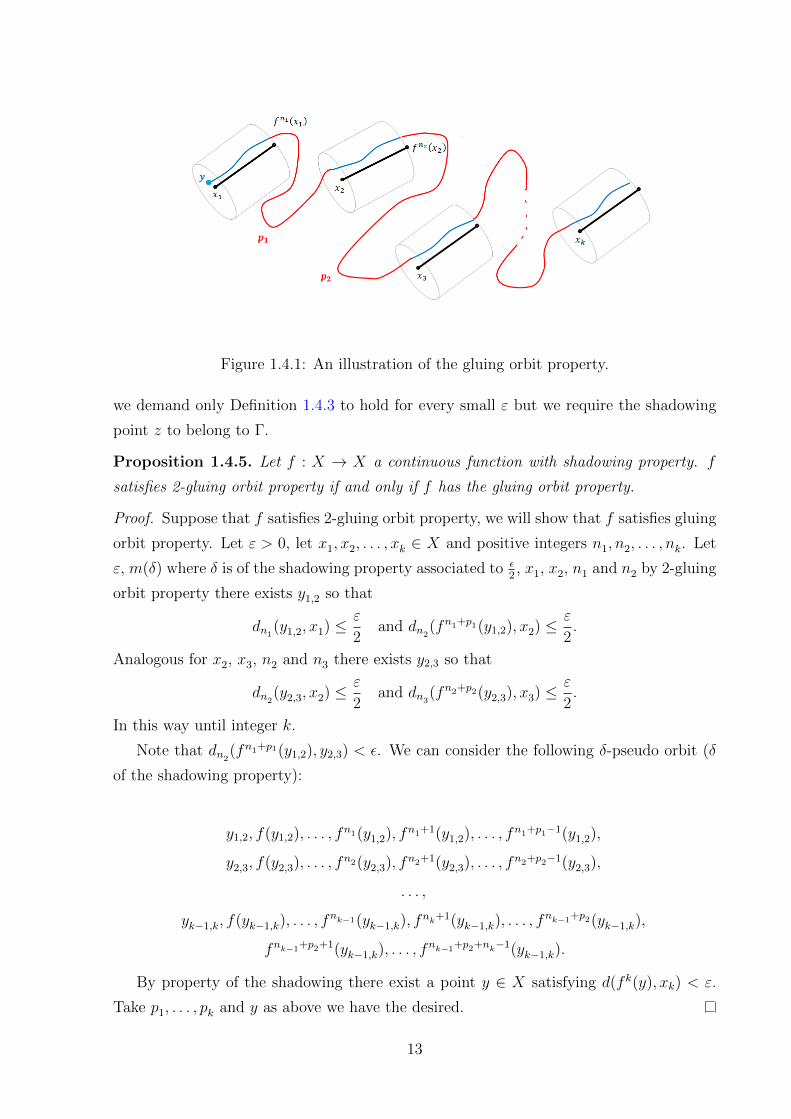
Figure 1.4.1: An illustration of the gluing orbit property.
we demand only Definition 1.4.3 to hold for every small ε but we require the shadowing
point z to belong to Γ.
Proposition 1.4.5. Let f : X → X a continuous function with shadowing property. f
satisfies 2-gluing orbit property if and only if f has the gluing orbit property.
Proof. Suppose that f satisfies 2-gluing orbit property, we will show that f satisfies gluing
orbit property. Let ε > 0, let x1, x2, . . . , xk ∈ X and positive integers n1, n2, . . . , nk. Let
ε, m(δ) where δ is of the shadowing property associated to ε2, x1, x2, n1 and n2 by 2-gluing
orbit property there exists y1,2 so that
dn1(y1,2, x1) ≤ ε
2and dn2
(fn1+p1(y1,2), x2) ≤ ε
2.
Analogous for x2, x3, n2 and n3 there exists y2,3 so that
dn2(y2,3, x2) ≤ ε
2and dn3
(fn2+p2(y2,3), x3) ≤ ε
2.
In this way until integer k.
Note that dn2(fn1+p1(y1,2), y2,3) < ε. We can consider the following δ-pseudo orbit (δ
of the shadowing property):
y1,2, f(y1,2), . . . , fn1(y1,2), fn1+1(y1,2), . . . , fn1+p1−1(y1,2),
y2,3, f(y2,3), . . . , fn2(y2,3), fn2+1(y2,3), . . . , fn2+p2−1(y2,3),
. . . ,
yk−1,k, f(yk−1,k), . . . , fnk−1(yk−1,k), f
nk+1(yk−1,k), . . . , fnk−1+p2(yk−1,k),
fnk−1+p2+1(yk−1,k), . . . , fnk−1+p2+nk−1(yk−1,k).
By property of the shadowing there exist a point y ∈ X satisfying d(fk(y), xk) < ε.
Take p1, . . . , pk and y as above we have the desired.
13

1.5 Reparametrization gluing orbit properties for
continuous flow
In this Section we define a notion of gluing orbit property for continuous flows
and reparametrized gluing orbit property for continuous flows, wich is weaker than
specification. The notion of reparametrized gluing orbit property was introduced in [6].
First we define gluing orbit property for continuous flow.
Definition 1.5.1. Let X ∈ X0(M), (Xt)t a continuous flow generated by X we say that
(Xt)t satisfies gluing orbit property if for any ε > 0 there exists K = K(ε) ∈ R+ such that
for any points x1, x2, . . . , xk in M and times t1, . . . , tk ≥ 0 there are p1, . . . , pk−1 ≤ K(ε)
and a point y ∈M so that
d(Xt(y), Xt(x1)) < ε, ∀ t ∈ [0, t1]
and
d(Xt+∑i−1
j=0 tj+pj(y), Xt(x1)) < ε, ∀ t ∈ [0, ti]
for every 2 ≤ i ≤ k.
Denote byRep the set of all increasing homeomorphisms τ : R→ R satisfying τ(0) = 0.
τ is called reparametrization. Fixing ε > 0, we define the set
Rep(ε) = τ ∈ Rep :| τ(s)− τ(t)
s− t− 1 |< ε, s, t ∈ R
of the reparametrizations ε-close to the identity. It is, the reparametrization τ belongs to
Rep(ε) whenever the slopes formed by any two points in its graph belong to the interval
(1− ε, 1 + ε).
Now we define the reparametrized gluing orbit property for flow.
Let X ∈ X(M), (Xt)t a continuous flow generated by X. We say that (Xt)t satisfies
reparametrized gluing orbit property if for any ε > 0 there exists K = K(ε) ∈ R+ such
that for any points x1, . . . , xk in M and times t1, . . . , tk ≥ 0, there are p1, . . . , pk−1 ≤ K(ε),
a reparametrization τ ∈ Rep(ε) and a point y ∈M so that
d(Xτ(t)(y), Xt(x1)) < ε, ∀ t ∈ [0, t1]
and
d(Xτ(t+∑i−1
j=0 tj+pj)(y), Xt(x1)) < ε, ∀ t ∈ [0, ti]
for every 2 ≤ i ≤ k.
This notion is an extension of the original notion of gluing introduced by Bomfim and
Varandas in [7].
Note that if τ ∈ Rep(ε) and p1 is as above on the definition of gluing orbit property,
then τ(t+ p1)− τ(t) ≤ (1 + ε)p1 ≤ (1 + ε)K(ε).
14

1.6 Pressure, entropy and mean dimensions
In this section we recall two important measurements of topological complexity, namely
the concepts of topological entropy and metric mean dimension, and introduce a relative
notion of the later. Our interest in the second notion is that, while a dense set of
homeomorphisms on a compact Riemannian manifold have positive and finite topological
entropy (by denseness of C1-diffeomorphisms) it is known that typical homeomorphisms
may have infinite topological entropy. In opposition, metric mean dimension is always
bounded by the dimension of the compact manifold and can be seen as a smoothened
measurement of topological complexity as we now detail.
Topological pressure
Let (X, d) be a compact metric space and ψ ∈ C0(X,R). Given ε > 0 and n ∈ N,
we say that E ⊂ X is (n, ε)-separated if for every x 6= y ∈ E it holds that dn(x, y) > ε,
where dn(x, y) = maxd(f j(x), f j(y)); j = 0, . . . , n− 1 is the Bowen’s distance. Bowen’s
dynamical balls are the sets Bn(x, ε) = y ∈ X : dn(x, y) < ε. The topological pressure
of f with respect to ψ is defined by
Ptop(f, ψ) = limε→0
lim supn→∞
1
nlog
(supE
∑x∈E
eSnψ(x)
),
where Snψ(x) =∑n−1
j=0 ψ(f j(x)) and the supremum is taken over every (n, ε)-separated
sets E contained in X. In the case that ψ ≡ 0, if s(n, ε) denotes the maximal cardinality
of a (n, ε)-separated subset of X, then the topological entropy is defined by
htop(f) = limε→0
lim supn→∞
1
nlog s(n, ε).
The previous notion does not depend on the metric d and is a topological invariant.
Moreover, by the classical variational principle for the pressure, it holds that Ptop(f, ψ) =
suphµ(f) +∫ψdµ : µ ∈ M(f). However, the topological entropy of C0-generic
homeomorphisms on a closed manifold of dimension at least two is infinite [53] (the
same holds for the topological pressure as a consequence of the variational principle), in
which case neither the topological preassure nor topological entropy can distinguish such
dynamics.
Topological and metric mean dimension
Gromov [21] proposed an invariant for dynamical systems called mean dimension, that
was further studied by Lindenstrauss and Weiss [29]. The upper and lower metric mean
15

dimension, which may depend on the metric, are defined in [28, 29] by
mdim(f) = limε→0
limn→∞1n
log s(n, ε)
− log ε
and
mdim(f) = limε→0
limn→∞1n
log s(n, ε)
− log ε,
respectively. If the supremum and infimum limits agree, we denote the common value by
mdim(f). Observe that the latter quantitities are only meaningful whenever f has infinite
topological entropy. In the case that the metric space satisfies a tame growth of covering
numbers, the metric mean dimension satisfies a variational principle involving a concept
of measure theoretical mean dimension (cf. [28]).
Relative metric mean dimension
Since we aim to describe the topological complexity of (not necessarily compact) f -
invariant subsets we now introduce a concept of relative metric mean dimension using
a Caratheodory structure. Let Z ⊂ X be a f -invariant Borel set. Given s ∈ R and
ψ ∈ C0(X,R) define
Q(Z, ψ, s,Γ) =∑
Bni(xi,ε)∈Γ
e−s ni +Sniψ(Bni(xi,ε)) and M(Z, ψ, s, ε,N)=inf
ΓQ(Z, ψ, s,Γ) ,
where Sniψ(Bni
(xi, ε)) := supx∈Bni(xi,ε)
∑ni−1
k=0 ψ(fk(x))) and the infimum is taken
over all countable collections Γ = Bni(xi, ε)i that cover Z and so that ni ≥ N .
Since the function M(Z, ψ, s, ε,N) is non-decreasing in N the limit m(Z, ψ, s, ε) =
limN→∞
M(Z, ψ, s, ε,N) does exist. Then let
PZ(f, ψ, ε) = infs ∈ R : m(Z, ψ, s, ε) = 0 = sups ∈ R : m(Z, ψ, s, ε) =∞.
The existence of PZ(f, ψ, ε) follows by the Caratheodory structure [40]. The (relative)
topological pressure of f on Z with respect to ψ is defined by
PZ(f, ψ) = limε→0
PZ(f, ψ, ε).
We set hZ(f, ε) = PZ(f, 0, ε) for every ε > 0 and define the relative entropy of f on Z by
hZ(f) = PZ(f, 0) (which corresponds to the potential ψ ≡ 0).
The upper and lower relative metric mean dimension of Z are given by
mdimZ(f) = limε→0hZ(f, ε)
− log εand mdimZ(f) = limε→0
hZ(f, ε)
− log ε
respectively. If the previous limits coincide, we represent simply by mdimZ(f) and refer
to this as the relative metric mean dimension of Z.
16
Definition 1.6.1. We say that the f -invariant subset Z ⊂ X has full topological entropy
if hZ(f) = htop(f). We say that the f -invariant subset Z ⊂ X has full metric mean
dimension if mdimZ(f) = mdim(f) and mdimZ(f) = mdim(f).
Remark 1.6.2. If f : X → X is a continuous map on a compact metric space and ψ ∈C0(X,R) then Ptop(f, ψ) = PX(f, ψ). Moreover, if the limits exist and coincide then
mdimX(f) = mdim (f). This follows from the fact that hX(f, ε) = htop(f, ε) for any
ε > 0, which can be read from the proof of [41, Proposition 4 ] (actually in [41] the
authors use the definition of entropy using coverings and prove that hX(f,U) = htop(f,U)
for every open cover U).
Remark 1.6.3. The notion of Hausdorff dimension also involves a Caratheodory structure,
associated to the function Q(Z, s,Γ) =∑
Bni (xi,ε)∈Γ diam(Bni(xi, ε))
s (see [40, Section 6]).
Inspired by [4] we expect that for continuous and transitive maps on the interval (these
satisfy the gluing orbit property, [1]) the set of points with historic behavior is either
empty or has Hausdorff dimension equal to one. We neither claim nor prove this fact
here.
We use the following generalization of Katok’s formula for pressure:
Proposition 1.6.4. [52, Proposition 2.5] Let (X, d) be a compact metric space, f be
a continuous map on X and µ be an f -invariant, ergodic probability. Given ε > 0,
γ ∈ (0, 1) and ψ ∈ C0(X,R) set Nµ(ψ, γ, ε, n) = infE∑
x∈E exp∑n−1
i=0 ψ(f i(x)), where
the infimum is taken over all sets E that (n, ε)-span a set Z with µ(Z) ≥ 1− γ. Then
hµ(f) +
∫ψdµ = lim
ε→0lim infn→∞
1
nlogNµ(ψ, γ, ε, n).
Remark 1.6.5. Given ε > 0 and ϕ ∈ C0(X,Rd), the variation in balls of radius ε is
var(ϕ, ε) = sup| ϕ(x)− ϕ(y) |: d(x, y) < ε.
Since X is compact then var(ϕ, ε)→ 0 as ε→ 0. As ϕ : X → Rd is continuous (hence
uniformly continuous) and f is continuous then for every ε > 0 there exists δ > 0 such
that ‖ 1n
∑n−1i=0 ϕ(f i(x))− 1
n
∑n−1i=0 ϕ(f i(y))‖ < ε whenever dn(x, y) < δ.
17

Chapter 2
Statement of the main results
In this chapter we expose our results. Before, recall that we denote by Homeo0(X) the
space of homeomorphisms on X homotopic to the identity and Homeo0,λ(X) the space of
homeomorphisms on X homotopic to the identity that area-preserving.
2.0.1 Points with historic behavior for maps with gluing orbit
property
The results in this section, despite their own interest, will be key technical ingredients
in the characterization of rotation sets for homeomorphisms on tori. These applications
motivate to describe the set of points with historic behavior for observables taking values
on Rd, d ≥ 1, and dynamical systems with the gluing orbit property (see Subsection 1.4
for the definition).
Let X denote a compact metric space, f : X → X be a continuous map, d ≥ 1 be
an integer and ϕ : X → Rd be a continuous observable. Given x ∈ X, let us denote
by Vϕ(x) the (connected) set obtained as accumulation points of ( 1n
∑n−1j=0 ϕ(f j(x)))n≥1.
In the higher dimensional setting context, (d > 1) the set Vϕ =⋃x∈X Vϕ(x) ⊂ Rd of
all vectors obtained as pointwise limits of Birkhoff averages does not need connected or
convex.
A point x ∈ X has historic behavior for ϕ (also known as exceptional, irregular or
non-typical behavior) if the limit limn→∞1n
∑n−1j=0 ϕ(f j(x)) does not exist. Moreover, we
say that x ∈ X has wild historic behavior if Vϕ(x) and Vϕ(x) = Vϕ and we denote
Xwildϕ,f := x ∈ X : Vϕ(x) = Vϕ. In rough terms, a point has wild historic behavior if the
Birkhoff averages have the largest oscillation in Vϕ. We say that B ⊂ X is Baire residual
if it contains a countable intersection of open and dense subsets of X. Our first result
asserts that, if non-empty, the set of points with wild historic behavior is large from the
18

category point of view.
Theorem A. Let X be a compact metric space, let f : X → X be a continuous map with
the gluing orbit property and let ϕ : X → Rd be continuous. Then:
1. either there is v ∈ Rd so that limn→∞1n
∑n−1j=0 ϕ(f j(x)) = v for all x ∈ X,
2. or the set of points x ∈ X so that the sequence ( 1n
∑n−1j=0 ϕ(f j(x)))n≥1 accumulates
in a non-trivial connected subset of Rd is Baire residual on X.
Moreover, if Xϕ,f 6= ∅ then Vϕ is connected and the set of points with wild historic behavior
is a Baire residual subset of X.
The next result establishes that the set of points with historic behavior has also large
complexity, now measured in terms of topological entropy and metric mean dimension.
We refer the reader to Subsection 1.6 for the notions of full topological pressure and full
metric mean dimension.
Theorem B. Let f : X → X be a continuous map with the gluing orbit property on
compact metric space X and let ϕ : X → Rd be a continuous observable. Assume that
Xϕ,f 6= ∅. Then Xϕ,f carries full topological pressure and full metric mean dimension.
Under the previous assumptions, the set of points with historic behavior for ϕ is empty
if and only if there exists v ∈ Rd so that∫ϕdµ = v for every f -invariant probability
measure (cf. Lemma 3.2.1). We also prove the following:
Corollary A. Let X be a compact Riemannian manifold. There exists a C0-Baire residual
subset R ⊂ Homeo(X)×C0(X,Rd) so that either htop(f) = 0 or Xϕ,f has full topological
entropy for any pair (f, ϕ) ∈ R.
2.0.2 Pointwise rotation sets of homeomorphisms on the torus
T2
In this section we address the questions concerning the pointwise rotation sets of torus
homeomorphisms homotopic to the identity (check Section 1.2 for more details about
rotation set). We note that the pointwise rotation set may fail to be connected and all
(see e.g. [30, Example 1]). Our first results ensure that there is a large set of points with
non-trivial pointwise rotation set of x. First we consider in the case of volume preserving
homeomorphisms.
Theorem C. There exists a Baire residual subset R1 ⊂ Homeo0,λ(T2) so that, for every
f ∈ R1 and every lift F : R2 → R2 of f :
19

1. the pointwise rotation set ρp(F ) is connected;
2. the set of points x ∈ T2 such that ρ(F, x) is non-trivial (ie, ρ(F, x) 6= v for some v)
which coincide with ρp(F ) is a Baire residual subset of T2, it carries full topological
pressure and full metric mean dimension in T2.
Now we describe the counterpart of Theorem C on the space Homeo0(T2) of
homeomorphisms homotopic to the identity. Consider the set
A =f ∈ Homeo0(T2) : int(ρ(F )) 6= ∅
.
All homeomorphisms in A have positive topological entropy [30]. Let Ω(f) denote
as usual the non-wandering set of f and consider the finite decomposition of Ω(f) in its
chain recurrent classes. We prove the following:
Theorem D. There exists a Baire residual subset R2 ⊂ A so that, for every f ∈ R2 there
exists a positive entropy chain recurrent class Γ ⊂ Ω(f) such that the set of points x ∈ Γ
for which ρ(F, x) is non-trivial is a Baire residual subset of Γ that carries full topological
entropy and full metric mean dimension in Γ.
We observe that the Theorem C is due to specification, but in case dissipative, the
Theorem D, specification is not sufficient, thus we need of the concept of gluing orbit
property.
2.0.3 On the rotation set of homeomorphisms on the torus Td
(d ≥ 2)
The shape of the different rotation sets for an homeomorphism f homotopic to
identity on the torus Td have drawn the attention since these have been introduced (see
Subsection 1.2 for definitions). Focusing first on connectedness, the rotation set ρ(F )
(and each pointwise rotation set of x, denoted by ρ(F, x), where x ∈ π−1(x)) is a compact
and connected set in Rd [30, 35]. However, the pointwise rotation set ρp(F ) may fail to
be connected even when d = 2 [30]. As for convexity, ρ(F ) is convex when d = 2, but
there are higher dimensional examples where it fails to be convex [35]. Our next result
ensures that rotation sets of torus homeomorphisms are typically convex.
Theorem E. For every d ≥ 2:
1. there exists a Baire residual subset R3 ⊂ Homeo0,λ(Td) so that ρ(F ) is convex, for
every lift F of a homeomorphism f ∈ R3; and
20

2. there exists a Baire residual subset R4 ⊂ Homeo0(Td) so that ρ(F |π−1(Γ)) is convex,
for every chain recurrent class Γ ⊂ Ω(f) and every lift F of f ∈ R4.
While the rotation set is always connected, in the case of dissipative homeomorphisms
Homeo0(Td) (e.g. Morse-Smale diffeomorphisms on the torus) the pointwise rotation set
need not to be connected. If the pointwise rotation set is connected then one can hope
that the “local” convexity statement in item (2) can be used to prove the convexity of
the rotation set.
2.0.4 Points with historic behavior for a flows with
reparametrized gluing orbit property
Our next results describe the set of points with historic behavior for continuous flows
with the reparametrized gluing orbit property. Before some definitions.
Let M be an n-dimensional Riemaniann closed manifold with n ≥ 2. Let L > 0,
denote X0(M) the set of continuous vector fields X : M → TM and X0,1L (M) the set of
Lipschitz continuous vector fields X : M → TM with Lipschitz constant ≤ L. We endow
X0(M) and X0,1L (M) with the C0-topology, ie, given X, Y ∈ X0,1
L (M), X is ε-close Y if
maxx∈M ‖X(x)−X(y)‖ < ε. We denote by (Xt)t the flow associated to X ∈ X0,1L (M).
Let M a compact metric space, X ∈ X0(M), (Xt)t a flow generated by X and ϕ :
M → Rd continuous. Define the irregular set for (Xt)t by
Iϕ =x ∈M : lim
t→∞
1
t
∫ t
0
ϕ Xs(x) ds does not exist. (2.0.1)
Recall that A ⊂ M is (Xt)t-invariant if Xt(A) = A, for all t ∈ R and that a finite
measure µ on M is (Xt)t-invariant if µ(Xt(A) = A, for every measurable A ⊂ M and
t ∈ R. Also note that Iϕ has zero measure with respect to any Φ-invariant measure.
A point x ∈ M has historic behavior for ϕ (on the flow) if the limit limt→∞1t
∫ t0ϕ
Xs(x)ds does not exist.
For d ≥ 2, define
Lϕ = ~v ∈ Rd : Aϕ(~v) 6= ∅
where
Aϕ(~v) := x ∈M : limt→∞
1
t
∫ t
0
ϕ Xs(x) ds = ~v.
We prove, for continuous flow with reparametrized gluing orbit property (check
Subsection 1.5 for definition) that:
Theorem F. Let Y ∈ X0(M). If (Yt)t is a flow generated by Y with the reparametrized
gluing orbit property on ∆ compact and invariant and ϕ : M → Rd is continuous, then
21

the irregular set of ϕ either trivial or Baire residual subset on ∆. In other word, if the
irregular set of ϕ is non-trivial, then the set of points with historic behavior is a Baire
residual subset of ∆.
As consequence we have the following:
Corollary B. Let X ∈ X0(M). If (Xt)t is a flow generated by X with the reparametrized
gluing orbit property on Γ where Γ is a chain recurrent class on Ω((Xt)t) and ϕ : M → Rd
is continuous, then the irregular set of ϕ either trivial or Baire residual subset on Γ.
In [6] is proved that: If M be a compact manifold there exists a C0-residual subset
of vector fields X in X0(M) so that every such vector field X has reparametrized gluing
orbit property in chain recurrent class Γ ⊂ Ω((Xt)t). This ensure the following.
Corollary C. Let M be a compact manifold. There exists a C0-residual subset of vector
fields X in X0(T2) so that if (Xt)t is a generated flows by X, ϕ : M → Rd continuous and
Γ ⊂ Ω((Xt)t) is a chain recurrent class, then the irregular set Iϕ is either trivial or Baire
residual subset of Γ.
2.0.5 Points with historic behavior for a suspension flow and
rotation set
Let M be a measurable space and f : M → M a measurable map and a measurable
roof function r : Σ −→ [0,∞). We can define the suspension flows (Xt)t over f by
Xt(x, s) = (x, s+ t),
whenever the expression is well defined, acting on
Mr = (x, t) ∈ X × R+ : 0 ≤ t ≤ r(x)/ ∼
where ∼ is the equivalence relation given by (x, r(x)) ∼ (f(x), 0) for all x ∈ Σ. Note
that the coordinates of (Xt)t coincides with the flow along the vertical direction. More
precisely,
Xt(x, s) =(fk(x), s+ t−
k−1∑j=0
r(f j(x))),
where k = k(x, s, t) is determined by∑k−1
j=0 r(fj(x)) ≤ s+ t <
∑kj=0 r(f
j(x)).
Our next results describe the set of points with historic behavior for suspension flows
over a map with gluing orbit property. First, consider the following number:
22

Cξ = supn≥1
supy∈B(x,n,ξ)
‖SnR(x)− SnR(y)‖ <∞, satisfy limξ→0
Cξ = 0, (2.0.2)
The condition under Cξ is a bounded distortion property for the roof function. It is
not hard to check it holds e.g. for Holder continuous observables and uniformly expanding
dynamics. So, we have:
Theorem G. Let M be an n-dimensional Riemaniann closed manifold, f ∈ Homeo(M)
with gluing orbit property and ϕ : Mr → Rd continuous. Suppose that (Xt)t is a suspension
flow over f satisfying condition (2.0.2). Then, the irregular set of ϕ either trivial or Baire
residual subset on M . In other word, if Iϕ is non-trivial, then the set of points with historic
behavior is a Baire residual.
Now, consider the suspension flows when f ∈ Homeo0(T2). Since that f admits a lift
F we can then define a suspension flow (Yt)t over F so that (Yt)t is a lift of (Xt)t. The
roof function in (Yt)t is R : R2 −→ (0,∞), defined by R(v) = r(π(v)). In this context, we
define the suspension flow to (Yt)t acting on
(x, t) ∈ Mr := (x, t) ∈ R2 × R+ : 0 ≤ t ≤ R(x)/ ∼,
where R : R2 −→ (0,∞) is the roof function and ∼ is the equivalence relation given by
(x,R(x)) ∼ (F (x), 0).
Passeggi in [39] proved that there exists an open and dense set D ⊂ Homeo0(T2) such
that for every f ∈ D the rotation set ρ(F ) is a polygon with finite rational vertices. So,
we have the following:
Theorem H. Let f ∈ Homeo(T2). Suppose that f ∈ D, that (Xt)t is a suspension flow
over f and the roof function r is coboundary, then the rotation set ρ((Yt)t) is a polygon
rational, (where (Yt)t is a lift of (Xt)t). Moreover, if r is cohomologous to a rational
number, then the polygon has rational vertices.
2.0.6 Overview of the proof
Theorems A and B provide three distinct measurements of the topological complexity
of the set of points with historic behavior. Their proofs use the construction of points with
non-convergent Birkhoff averages by exploring the oscillatory behavior in the Birkhoff
averages of points that shadow pieces of orbits that are typical for invariant measures
with different space averages. The existence of such points is granted by the gluing orbit
property.
23

If, on the one hand, the proof of Theorems A and B are inspired by [4, 25, 52], the
arguments in the proof of Theorem B is much more challenging and presents novelties on
how to construct a ‘large amount’ of points whose finite pieces of orbits up to time n have
a controlled behavior and that are separated by the dynamics. This is crucial to estimate
topological pressure and metric mean dimension. While the construction of points with
non-convergent behavior can be obtained as a consequence of the gluing orbit property,
it is natural to inquire on the control on the number of such distinct orbits (measured
in terms of (n, ε)-separability). We overcome this issue by selecting of a large amount of
orbits that are glued the same (bounded) time. Since this bound depends on ε, so does
the estimates on the number of (n, ε)-separated points with controlled recurrence. This
requires shadowing times to be chosen large in order to compensate the latter. In [15] the
authors obtain similar flavored results using shadowing. Although both occur properties
hold C0-generically there are several examples that satisfy the gluing orbit property and
fail to satisfy shadowing, which justifies our approach.
The first ingredient in the proof of Theorems C and D relies on the fact that each chain
recurrent class of C0-generic homeomorphisms satisfy the gluing orbit property. This will
ensure that any connected subset of the rotation set can be realized by the rotation set
along the orbit of a point relies on any vectors. Such a reconstruction of rotation vectors
as the orbit of a single point is formalized in Theorems A and B. In comparison with the
former, extra difficulties arise from the fact that the dynamics and the observables are
not decoupled and the fact that, in the case of dissipative homeomorphisms, the chain
recurrent classe(s) that concentrate topological pressure vary as the potential changes.
One could ask whether the Baire generic conclusion of Theorem D could extend to a
generic set of points in the whole chain-recurrent set (or the non-wandering set). For
instance, it is easy to construct an Axiom A diffeomorphism f on S2 so that Ω(f) =
p1∪Λ∪p2, where p1 is a repelling fixed point, p2 is an attracting fixed point and Λ is
an horseshoe. Recall that f is an Axiom A diffeomorphism if the set of periodic points is
dense in the non-wandering set Ω(f) and Ω(f) is hyperbolic (we refer, for instance, to [47]
for the construction of such examples). The existence of a filtration for homeomorphisms
C0-close to f imply that the Baire generic subset in the statement of Theorem D can only
be contained in a neighborhood of the basic piece Λ for all C0-close homeomorphisms.
Moreover, the assertion concerning positive entropy seems optimal. Indeed, it may occur
that there exists a unique chain recurrent class of largest positive topological entropy and
whose (restricted) rotation set have empty interior or even reduce to a point, in the case
of pseudo-rotations. Related constructions include [17, 45].
Theorems E relies on the fact that under the specification, or the gluing orbit property,
24
the space of periodic measures is dense in the space of all invariant measures. Under any
of these assumptions, the generalized rotation set coincides with the rotation set obtained
by means of invariant measures, thus it is convex.
The Theorem F and G are an attempt to generalize from Theorem A, the strategy to
proof of the F is also similar. Finally, the Theorem H is a relationship between suspension
flow and rotation set.
25

Chapter 3
The set of points with historic
behavior
The main goal of this chapter is to prove Theorems A and B, which claim that the
set of points with historic behavior for continuous maps with the gluing orbit property is
topologically large. Actually, this is established by means of three different measurements
of topological complexity: Baire genericity, full topological entropy and full metric mean
dimension. The arguments involved in the proofs of Theorems A and B are substantially
different and their proofs occupy Sections 3.1 and 3.2, respectively.
3.1 Baire genericity of historic behavior and proof of
the Theorem A
This section is devoted to the proof of Theorem A, whose strategy is strongly inspired
by [2, 25]. The differences lie on the fact that, due to the higher dimensional features of
observables, we need to restrict to connected subsets in the set of all accumulation vectors,
and that we have transition time functions instead of a determined time to shadow pieces
of orbits (see Remark 3.1.3 below).
Let f : X → X be a continuous map with the gluing orbit property on a compact
metric space X and let ϕ : X → Rd be a continuous function so that Vϕ is non-trivial.
Let ∆ ⊂ Vϕ a non-trivial connected set, define
X∆ :=x ∈ X : ∆ ⊂ Vϕ(x)
. (3.1.1)
Note that for all ∆ ⊂ Vϕ hold that X∆ ⊂ Xϕ,f . Theorem A will be a consequence of the
following:
26
Proposition 3.1.1. Let X be a compact metric space, f ∈ Homeo(X) satisfy the gluing
orbit property, ϕ : X → Rd be continuous such that Vϕ is non-trivial. If ∆ ⊂ Vϕ is a
non-trivial connected set, then X∆ is Baire residual in X.
Remark 3.1.2. The set Vϕ corresponds to the pointwise rotation set of ϕ, which needs not
be connected in general. Since Baire residual subsets are preserved by finite intersection, a
simple argument by contradiction ensures that under the assumptions of Proposition 3.1.1
the set Vϕ is connected. In particular, since Vϕ(x) ⊂ Vϕ, the latter ensures that Xwildϕ,f :=
x ∈ X : Vϕ(x) = Vϕ. is Baire residual.
[Proof of the Proposition 3.1.1]: The remaining of the section is devoted to the proof of
Proposition 3.1.1. Let D ⊂ X be countable and dense. Let ε > 0 be arbitrary and fixed
and let m(ε) be given by the gluing orbit property (cf. Section 1.4). As Vϕ is non-trivial,
then Vϕ is not a singleton. Let ∆ ⊂ Vϕ be a non-trivial connected set and, for any k ≥ 1
let (vk,i)1≤i≤ak be a 1k-dense set of vectors in ∆ so that
‖vk,i+1 − vk,i‖ <1
kfor 1 ≤ i ≤ ak and ‖vk,ak − vk+1,1‖ <
1
k. (3.1.2)
For w ∈ Vϕ, δ > 0, n ∈ N let
P (w, δ, n) =x ∈ X :
∥∥ 1
n
n−1∑i=0
ϕ(f i(x))− w∥∥ < δ
.
Given k ≥ 1 and 1 ≤ i ≤ ak, let δk,ik≥1,1≤i≤ak be a sequence of positive real and
nk,ik≥1,1≤i≤ak be a sequence of integers tending to zero and infinity, respectively, so that
δ1,1 > δ1,2 > · · · > δ1,a1> δ2,1 > δ2,2 > · · · > δ2,a2
> . . . ,
n1,1 < n1,2 < · · · < n1,a1< n2,1 < n2,2 < · · · < n2,a2 < . . .
that nk,i mk, meaning here limk→∞mk
nk,i= 0, for all 1 ≤ i ≤ ak, where mk := m(ε/2bk),
with b0 = 0 and bk =∑
1≤i≤k ai, and P (vk,i, δk,i, nk,i) 6= ∅, for all k ≥ 1 and 1 ≤ i ≤ ak.
Note that bk →∞ as k →∞.
Given q ∈ D, k ≥ 1 and 1 ≤ i ≤ ak, let Wk,i(q) be a maximal (nk,i, 8ε)-separated
subset of P (vk,i, δk,i, nk,i). We index the elements of Wk,i(q) by xk,ij , for 1 ≤ j ≤ #Wk,i(q).
27

Choose also a strictly increasing sequence of integers N qk,ik≥1,1≤i≤ak so that
limk→ ∞
nk,i+1 +mk
N qk,i
= 0, for every 1 ≤ i ≤ ak − 1
limk→ ∞
nk+1,1 +mk+1
N qk,ak
= 0, for k ≥ 1 (3.1.3)
limk→ ∞
N q1,1(n1,1 +m1) + · · ·+N q
k,i(nk,i +mk)
N qk,i+1
= 0 for every , 1 ≤ i ≤ ak − 1, and
limk→ ∞
N q1,1(n1,1 +m1) + · · ·+N q
k,ak(nk,ak +mk)
N qk+1,i
= 0 for every , k ≥ 1
We shall omit the dependence of Wk,i(q) and N qk,i on q when no confusion is possible. The
idea is to construct points that shadow finite pieces of orbits associated with the vectors
vk,i repeatedly.
We need the following auxiliary construction. The gluing orbit property ensures that
for every xk,i := (xk,i1 , . . . , xk,iNk,i) ∈ (Wk,i)
Nk,i there exists a point y = y(xk,i) ∈ X and
transition time functions
pjk,i : WNk,i
k,i × R+ → N, j = 1, 2, . . . , Nk,i − 1
bounded above by m( ε
2bk−1+i ) ≤ mk so that
dnk,i(f ej(y), xk,ij ) <
ε
2bk−1+i, for every j = 1, 2, . . . , Nk,i − 1, (3.1.4)
where
ej =
0 if j = 1
(j − 1)nk,i +∑j−1
r=1 prk,i if j = 2, . . . , Nk,i.
(3.1.5)
Remark 3.1.3. For k and j as above we have that pjk,i = pjk,i(xk,i1 , xk,i2 , . . . , xk,iNk,i
, ε) is a
function that describes the time lag that the orbit of y = y(xk,i) takes to jump from a ε2k
-
neighborhood of fnk,i(xk,ij ) to a ε2k
-neighborhood of xk,ij+1, and it is bounded above by mk.
In contrast with the case when f has the specification property, the previous functions
need not be constant and, consequently, the collection of points of the form y = y(xk,i)
need not be 3ε-separated by a suitable iterate of the dynamics. For that reason, not
only an argument to select a ‘large set’ of distinguishable orbits would require to compare
points with the same transition times, which strongly differs from [2, 25].
We order the family Wk,ik≥1,1≤i≤ak lexicographically: Wk,i ≺ Ws,j if and only if k ≤ s
and i ≤ j whenever k = s. We proceed to make a recursive construction of points in a
neighborhood of q that shadow points Nk,i in the family Wk,i successively with bounded
time lags in between. More precisely, we construct a family Lk,i(q)k≥0,1≤i≤ak of sets
28

(guaranteed by the gluing orbit property) contained in a neighborhood of q and a family
of positive integers lk,ik≥0,1≤i≤ak (also depending on q) corresponding to the time during
the shadowing process. Set:
• L0,i(q) = q and l0,i = N0,in0,i = 0;
• L1,1(q) = z = z(q, y(x1,1)) ∈ X : x1,1 ∈ WN1,1
1,1 and l1,1 = p01,1 + t1,1 with
t1,1 = N1,1n1,1 +∑N1,1−1
r=1 pr1,1, where z = z(q, y(x1,1)) satisfies d(z, q) < ε2
and
dt1,1(fp01,1(z), y(x1,1)) < ε
2, and y(x1,1) is defined by (3.1.4) and 0 ≤ p0
1,1 ≤ m( ε22
) is
given by the gluing orbit property;
• if i = 1
Lk,1(q) = z = z(z0, y(xk,1)) ∈ X : xk,1 ∈ WNk,1
k,1 and z0 ∈ Lk−1,ak−1, and lk,1 =
lk−1,ak−1+ p0
k,1 + tk,1, with tk,1 = Nk,1nk,1 +∑Nk,1−1
r=1 prk,1, where the shadowing point
z satisfies
dlk−1,ak−1(z, z0) <
ε
2bk−1+1and dtk,1(f
lk−1,ak−1+p0k,1(z), y(xk,1)) <
ε
2bk−1+1.
• if i 6= 1
Lk,i(q) = z = z(z0, y(xk,i)) ∈ X : xk,i ∈ WNk,i
k,i and z0 ∈ Lk,i−1, and lk,i = lk,i−1 +
p0k,i + tk,i, with tk,i = Nk,ink,i +
∑Nk,i−1r=1 prk,i, where the shadowing point z satisfies
dlk,i−1(z, z0) <
ε
2bk−1+iand dtk,i(f
lk,i−1+p0k,i(z), y(xk,i)) <ε
2bk−1+i.
Figure 3.1.1: Construction of L1,1(q) and L1,2(q).
29

The previous points y = y(xk,i) are defined as in (3.1.4). By construction, for every
k ≥ 1 and 1 ≤ i ≤ ak − 1,
lk,i =k∑r=1
ar∑s=1
Nr,snr,s +k∑r=1
ar−1∑s=1
Nr,s−1∑t=0
ptr,s. (3.1.6)
Remark 3.1.4. Note that lk,i and tk,i are functions (as these depend on pjk,i) and, by
definition of Nk,i cf. (3.1.3), one has that‖lk,i‖Nk,i+1
≤∑k
r=1
∑ars=1Nr,s(nr,s+mr)
Nk,i+1tends to zero as
k →∞.
For every k ≥ 0, 1 ≤ i ≤ ak, q ∈ D and ε > 0 define
Rk(q, ε, i) =⋃
z∈Lk,i(q)
Blk,i
(z,
ε
2bk−1+i
)and R(q, ε) =
∞⋂k=0
ak⋂i=1
Rk(q, ε, i),
where Blk,i(x, δ) is the set of points y ∈ X so that d(fα(x), fα(y)) < δ for all iterates
0 ≤α≤ lk,i−1 − 1 and d(fβ(x), fβ(y)) ≤ δ for every lk,i−1 ≤ β ≤ lk,i − 1.
Consider also the sets
R =∞⋃j=1
⋃q∈D
R(q,1
j) =
∞⋃j=1
⋃q∈D
∞⋂k=0
ak⋂i=1
⋃z∈Lk,i(q)
Blk,i
(z,
1
j2bk−1+i
), (3.1.7)
and finally
R =∞⋂k=0
∞⋃j=1
⋃q∈D
ak⋂i=1
⋃z∈Lk,i(q)
Blk,i
(z,
1
j2bk−1+i
). (3.1.8)
It is clear from the construction that R(q, ε) ⊂ B(q, ε) for every q ∈ D and ε > 0, and
that R ⊂ R. The following lemma, identical to Propositions 2.2 and 2.3 in [25], ensures
that R is a Baire generic subset of X.
Lemma 3.1.5. R is a Gδ-set and it is dense in X.
Proof. First we prove denseness. Since R ⊂ R, it is enough to show that R∩B(x, r) 6= ∅for every x ∈ X and r > 0. In fact, given x ∈ X and r > 0, there exists j ∈ N and
q ∈ D such that d(x, q) < 1/j < r/2. Given y ∈ R(q, 1j) it holds that d(q, y) < 1
jbecause
R(q, 1j) ⊂ B(q, 1
j). Therefore, d(x, y) ≤ d(x, q) + d(q, y) < 2/j < r. This ensures that
R ∩B(x, r) 6= ∅.Now we prove that R is a Gδ-set. Fix j ∈ N and q ∈ D. For any k ≥ 1 and 1 ≤ i ≤ ak,
consider the open set
Gk(q, ε, i) :=⋃
z∈Lk,i(q)
Blk,i
(z,
ε
2bk−1+i
)
30

and note that Gk(q, ε, i) ⊂ Rk(q, ε, i) for any k ≥ 1 and 1 ≤ i ≤ ak. We claim that
Rk(q, ε, i + 1) ⊂ Gk(q, ε, i) and Rk+1(q, ε, 1) ⊂ Gk(q, ε, ak), for any k ≥ 1 and 1 ≤ i ≤ak − 1. The claim implies that
∞⋃j=1
⋃q∈D
ak⋂i=1
Rk(q, ε, i) =∞⋃j=1
⋃q∈D
ak⋂i=1
Gk(q, ε, i),
and guarantees that R is a Gδ-set.
Now we proceed to prove the claim. We prove that Rk(q, ε, i + 1) ⊂ Gk(q, ε, i) for
any k ≥ 1 and 1 ≤ i ≤ ak − 1 (the proof of the Rk+1(q, ε, i) ⊂ Gk(q, ε, ak) is analogous).
Given y ∈ Rk(q, ε, i + 1), there exists z ∈ Lk,i+1(q) such that y ∈ Blk,i+1(z, 1
j2bk−1+(i+1) ).
By definition of Lk,i+1(q), there exists z0 such that dlk,i(z, z0) < 1
j2bk−1+(i+1) . Therefore,
dlk,i(y, z0) ≤ dlk,i(y, z) + dlk,i(z, z0) <1
j2bk−1+(i+1)+
1
j2bk−1+(i+1)=
1
j2bk−1+i
and consequently y ∈ Gk(q, ε, i). This proves the claim and completes the proof of the
lemma.
We must show that R ⊂ X∆, that is ∆ ⊆ Vϕ(x) for every x ∈ R. The proof
follows some ideas from [25, Proposition 2.1]. We provide a sketch of the argument for
completeness. Given x ∈ R fixed, for any k > 1, there exist integers j ∈ N, q ∈ D and
z ∈ Lk,i+1(q) such that
dlk,i+1(z, x) <
1
j2bk−1for every 1 ≤ i ≤ ak. (3.1.9)
We prove that ∆ ⊆ Vϕ(x). If v ∈ ∆, then for any k ≥ 1 there exists 1 ≤ ik ≤ ak such
that v ∈ B(vk,ik ,1k). We need the following:
Lemma 3.1.6. Take k ≥ 1 and 1 ≤ ik ≤ ak. If
Rqk,i := max
z∈Lk,i(q)
∥∥∥ lk,i−1∑r=0
ϕ(f r(z))− lk,i vk,i∥∥∥,
thenRq
k,i
lk,i→ 0, as k →∞.
Proof. Let k and i be as above, let xk,i ∈ (Wk,i)Nk,i and y = y(xk,i). Recall
that ‖∑n−1
i=0 ϕ(f i(x)) −∑n−1
i=0 ϕ(f i(y))‖ ≤ n var(ϕ, c) if dn(x, y) < c. Then, using
dnk,i(xk,it , f
et(y)) < 1
j2bk−1where et is defined in (3.1.5) with t ∈ 1, . . . , Nk,i we conclude
that ∥∥∥ nk,i−1∑r=0
ϕ(f r(xk,it ))−nk,i−1∑r=0
ϕ(f et+r(y))∥∥∥ ≤ nk,i var(ϕ,
1
j2bk−1).
31

Since xk,it ∈ Wk,i, we have that∥∥∥ nk,i−1∑r=0
ϕ(f et+r(y))− nk,i vk,i∥∥∥ ≤ nk,i(var(ϕ,
1
j2bk−1) + δk,i). (3.1.10)
We decompose the time interval [0, tk,i − 1] as follows:
Nk,i⋃t = 1
[et, et + nk,i − 1] ∪Nk,i−1⋃t = 1
[et + nk,i, et + nk,i + ptk,i − 1].
On the intervals [et, et + nk,i − 1] we will use the estimate (3.1.10), while in the time
intervals [et + nk,i, et + nk,i + ptk,i − 1] we use
∥∥∥ ptk,i−1∑r=0
ϕ(f et+nk,i+r(y))− ptk,i vk,i∥∥∥ ≤ mk(‖ϕ‖∞ + ‖vk,i‖) ≤ 2mk‖ϕ‖∞.
Therefore,∥∥∥ tk,i−1∑r=0
ϕ(f r(y))− tk,i vk,i∥∥∥ ≤ Nk,i nk,i(var(ϕ,
1
j2bk−1) + δk,i) + 2(Nk,i − 1)mk‖ϕ‖∞.(3.1.11)
On the other hand, by definition of Lk,i(q) that for every z ∈ Lk,i(q) there exist z0 ∈Lk,i−1(q) and y = y(xk,i) ∈ X such that
dlk,i−1(x, z) <
1
j2bk−1, dtk,i(y, f
lk,i−1+p0k,i(z)) <1
j2bk−1. (3.1.12)
By triangular inequality,∥∥∥ lk,i−1∑r=0
ϕ(f r(z))− lk,i vk,i∥∥∥ ≤ ∥∥∥ lk,i−1−1∑
r=0
ϕ(f r(z))− lk,i−1 vk,i
∥∥∥+
∥∥∥ lk,i−1+p0k,i−1∑r=p0k,i
ϕ(f r(z))− p0k,i vk,i
∥∥∥+
∥∥∥ tk,i−1∑r=lk,i−1+p0k,i
ϕ(f r(z))− tk,i vk,i∥∥∥,
where the first and second terms are bounded by 2lk,i−1‖ϕ‖∞ and 2mk‖ϕ‖∞, respectively.
Inequalities (3.1.11)-(3.1.12) imply∥∥∥ tk,i−1∑r=tk,i−1+p0k,i
ϕ(f r(z))− tk,i vk,i∥∥∥
≤∥∥∥ tk,i−1∑
r=0
ϕ(f lk,i−1+p0k,i+r(z))−tk,i−1∑r=0
ϕ(f r(y))∥∥∥+
∥∥∥ tk,i−1∑r=0
ϕ(f r(y))− tk,i vk,i∥∥∥
≤ tk,i var(ϕ,1
j2bk−1) +Nk,ink,i var(ϕ,
1
j2bk−1+ δk,i) + 2(Nk,i − 1)mk‖ϕ‖∞
32

and, consequently,
Rqk,i ≤ 2(lk,i−1 +Nk,imk)‖ϕ‖∞ + (tk,i +Nk,ink,i) var(ϕ,
1
j2bk−1) +Nk,ink,iδk,i.
By definition of Nk,i in (3.1.3) we obtain that Rqk,i/lk,i → 0 as k → ∞, which proves the
lemma.
Given z = z(z0, y(xk,i)) ∈ Lk,i+1(q) satisfying (3.1.9) with z0 ∈ Lk,i(q), by triangular
inequality we have dlk,i(z0, x) < 1
j2bk−1−1 . Thus,
∥∥∥ lk,ik−1∑r=0
ϕ(f r(x))− lk,ik vk,ik∥∥∥ (3.1.13)
≤∥∥∥ lk,ik−1∑
r=0
ϕ(f r(x))−lk,i
k−1∑
r=0
ϕ(f r(z0))∥∥∥+
∥∥∥ lk,ik−1∑r=0
ϕ(f r(z0))− lk,ik vk,ik∥∥∥
≤ lk,ik var(ϕ,1
j2bk−1−1) +Rq
k,ik.
Lemma 3.1.6 and the uniform continuity of ϕ ensures that∥∥∥ 1
lk,i
lk,i−1∑r=0
ϕ(f r(x))− v∥∥∥ ≤ ∥∥∥ 1
lk,i
lk,i−1∑r=0
ϕ(f r(x))− vk,ik∥∥∥+ ‖vk,ik − v‖ → 0 (3.1.14)
as k →∞ and, consequently, v ∈ Vϕ(x). This proves that ∆ ⊆ Vϕ(x).
Altogether we conclude that X∆ is a Baire residual subset of X, and finish the proof
of Proposition 3.1.1 and Theorem A.
3.2 Full topological pressure and metric mean
dimension
In this section we prove Theorem B. Assume that f is a continuous map with the
gluing orbit property on a compact metric space X, ϕ : X → Rd is continuous and
Xϕ,f 6= ∅. We will prove that mdimXϕ,f(f) = mdim(f), that mdimXϕ,f
(f) = mdim(f)
and htop(f) = hXϕ,f(f).
Actually we will prove that hXϕ,f(f, ε) = htop(f, ε) every ε > 0, which is a sufficient
condition. Fix ε > 0 and let m(ε) be given by the gluing orbit property.
3.2.1 Measures with large entropy and distinct rotation vectors
The proof explores the construction of an exponentially large (with exponential rate
close to topological entropy) number of points that oscillate between distinct vectors in Rd.
33

We use some auxiliary results. We say that a observable ϕ : X → Rd is cohomologous to a
vector if there exists v ∈ Rd and a continuous function χ : X → Rd so that ϕ = v+χ−χf ,
and denote by Cob the set of all such observables and by Cob its closure in the C0-topology.
Lemma 3.2.1. Assume that f has the gluing orbit property. The following are equivalent:
(i) Xϕ,f 6= ∅,
(ii) infµ∈Me(f)
∫ϕdµ < supµ∈Me(f)
∫ϕdµ, and
(iii) there exist periodic points p1, p2 of period k1, k2 respectively such that
1
k1
k1−1∑j=0
ϕ(f j(p1)) 6= 1
k2
k2−1∑j=0
ϕ(f j(p2)).
(iv) ϕ /∈ Cob.
(v) 1n
∑n−1j=0 ϕ f j does not converge uniformly to a constant.
Proof. Although this is similar to [52, Lemma 1.9] we include it for completeness.
(iii) ⇒ (iv): If ϕ ∈ Cob, then there is ϕk in Cob such that ϕ = limk→∞ ϕk. In
particular there exists vk ∈ Rd and χk so that
1
n
n−1∑j=0
ϕk(fj(x)) =
χk fn(x)
n− χk(x)
n+ vk (3.2.1)
for every x ∈ X. By Birkhoff’s ergodic theorem and dominated convergence theorem
Me(f) 3 µ 7→∫ϕdµ is constant, which contradicts (iii).
(iv)⇒ (v): If ϕ 6∈ Cob, then the sequence 1n
∑n−1j=0 ϕ f j is not uniformly convergent
to a vector v. Indeed, otherwise the sequence of continuous function (hn)n given by
hn = 1n
∑n−1i=0 (n− i)ϕ f i−1 satisfy the cohomological equation
hn(x)− hn(f(x)) = ϕ(x)− 1
n
n−1∑j=0
ϕ(f j(x)), ∀ x ∈ X
and so ϕ(x) = limn→∞[hn(x) − hn(f(x)) + 1n
∑n−1j=0 ϕ(f j(x))] ∈ Cob, leading to a
contradiction.
(v)⇒ (ii):
Let µ be an f -invariant probability measure and suppose that 1n
∑n−1j=0 ϕ(f j(x)) does
not converge uniformly to∫ϕdµ. There exists ε > 0 so that for every k ≥ 1 there
are nk ≥ k and xk ∈ X for which ‖ 1nk
∑nk−1j=0 ϕ(f j(xk)) −
∫ϕdµ‖ ≥ ε. Consider νk :=
34

1nk
∑nk−1j=0 δfj(xk) and let ν be a weak∗ accumulation point of the sequence (νk)k. Note that
ν is f -invariant. Choose k such that ‖ 1nk
∑nk−1j=0 ϕ(f j(xk))−
∫ϕdν‖ ≤ ε/2, so
∥∥∫ ϕdµ−∫ϕdν
∥∥ ≥ ∥∥∫ ϕdµ− 1
nk
nk−1∑j=0
ϕ(f j(xk))∥∥
−∥∥ 1
nk
nk−1∑j=0
ϕ(f j(xk))−∫ϕdν
∥∥ ≥ ε/2.
The conclusion follows from the ergodic decomposition theorem.
(ii) ⇒ (i): The construction in the proof of Theorem A ensures that if there exist
f -invariant measures µ1, µ2 so that∫ϕ dµ1 6=
∫ϕ dµ2, then Xϕ,f 6= ∅.
(i)⇒ (iii): If the limit limn→∞1n
∑n−1j=0 ϕ(f j(x)) does not exist for some x ∈ X, then
the empirical measures ( 1n
∑n−1j=0 δfj(x))n≥1 accumulate on f -invariant probability measures
µ1, µ2 so that∫ϕdµ1 6=
∫ϕdµ2. Now, the result follows as a simple consequence of the
weak∗ convergence and the fact that periodic measures are dense in the space of f -invariant
probability measures ([48, p102-104] proves the latter for maps with specification, but it
is straightforward to see that this holds for maps with the gluing orbit property, to see
5.0.4).
Lemma 3.2.2. Given ψ ∈ C0(X,R)and γ > 0 there are µ1, µ2 ∈ M1(f) so that µ1 is
ergodic,∫ϕdµ1 6=
∫ϕdµ2 and hµi(f) +
∫ψdµi > Ptop(f, ψ)− γ, for i = 1, 2.
Proof. By the variational principle there exists an ergodic µ1 ∈ M1(f) so that hµ1(f) +∫ψdµ1 > Ptop(f, ψ) − γ. As Xϕ,f 6= ∅ there is ν ∈ M1(f) satisfying
∫ϕdµ1 6=
∫ϕdν
(recall Lemma 3.2.1). Consider the family of measures
µt2 = tµ1 + (1− t)ν, t ∈ (0, 1) (3.2.2)
and observe that, by convexity, hµt2
(f) +∫ψdµt2 > Ptop(f, ψ) − γ, provided that t is
sufficiently close to one. the probability measure µ2 := µt2 satisfies the requirements of
the lemma.
Although the previously defined measures µ1, µ2 depend on the potential ψ ∈ C0(X,R)
we shall omit its dependence for notational simplicity.
3.2.2 Exponential growth of points with averages close to∫ϕdµi, i = 1, 2
Take the probability measures µ1, ν and µ2 given by Lemma 3.2.2, consider the
sequence ζkk of real numbers
ζk = max‖ ∫ ϕdµ1 −
∫ϕdν‖
2k, var(ϕ,
ε
2k), (3.2.3)
35
which tend to zero as k → ∞, and take mk = m( ε2k
). Given γ ∈ (0, 1), by Birkhoff’s
ergodic theorem one can choose n1k mk so that
mk/n1k → 0 as k →∞ (3.2.4)
such that µ1(Yk,1) ≥ 1− γ, where
Yk,1 =x ∈ X :
∥∥∥ 1
n
n−1∑j=0
ϕ(f j(x))−∫ϕdµ1
∥∥∥ < ζk for every n ≥ n1k
. (3.2.5)
The following lemma will be instrumental.
Lemma 3.2.3. There exists ε0 > 0 so that for any 0 < ε < ε0, there is a
collection S1kk so that every S1
k is a (n1k, 6ε) separated subset of Yk,1 and M1
k :=∑x∈S1
kexp(
∑n1k−1i=0 ψ(f i(x))) satisfies M1
k ≥ exp (n1k(Ptop(f, ψ, ε)− 4γ)).
Proof. The proof is a standard consequence of Proposition 1.6.4.
For any k ≥ 1, we now construct large sets of points S2k with averages close to
∫ϕdµ2
at large instants n2k ≥ 1 (to be defined below). First, as ν is ergodic, there exists xk ∈ X
and nk ≥ 1 so that∥∥ 1nk
∑nk−1j=0 ϕ(f j(xk)) −
∫ϕdν
∥∥ < ζk. Let t of the proof of Lemma
3.2.2, there are rk, sk ≥ 1 be integers satisfying
rkn1k
sknk→ t
1− tas k →∞. (3.2.6)
For any fixed k ≥ 1, any string (xk1, . . . , xkrk
) ∈ (S1k)rk and sk copies of the point xk, by
the gluing orbit property there exists y = y(xk1, . . . , xkrk
) ∈ X satisfying
dn1k(fai(y), xki ) < ε, and dnk
(f bj(y), xk) < ε
for every i = 1, 2, . . . , rk and j = 1, 2, . . . , sk, where
ai =
0 if i = 1
(i− 1)n1k +
∑i−1r=1 pk,r if i = 2, . . . , rk
and
bj =
ark + pk,rk if j = 1
(j − 1)nk +∑j−1
r=0 pk,rk+r + ark if j = 2, . . . , sk
where 0 ≤ pk,r ≤ m(ε) are the transition time functions defined similarly as in the proof of
Theorem A. We define the auxiliary set S2k as the set of points y obtained by the previous
process.
36
Remark 3.2.4. For every point x ∈ S2k we associate the size
n2k(·) := rkn
1k + sknk +
rk+sk−1∑r=1
pk,r(·),
of the finite piece of orbit, which is a function of (xk1, . . . , xkrk, xk, sk). In strong contrast
with the case when f satisfies the specification property, at this moment we can not claim
that the cardinality of S2k is large. Indeed, since n2
k varies with the elements in S2k then
the (n1k, 4ε)-separability of the points in S1
k is not sufficient to ensure the shadowing point
map (S1k)rk × xksk → X to be injective. This issue is solved by Lemma 3.2.5.
Now, for any j = (j1, j2, . . . , jrk+sk−1) ∈ Zrk+sk−1+ so that 0 ≤ ji ≤ m(ε) + 1 define
the set S2k(j) := x ∈ S2
k : pk,1 = j1, pk,2 = j2, . . . , pk,rk+sk−1 = jrk+sk−1. The size of
the finite orbit of all points in S2k(j) is constant and, by some abuse of notation, we will
denote it by
n2k(j) := rkn
1k + sknk +
rk+sk−1∑r=1
jr. (3.2.7)
It is not hard to check that (3.2.6) implies
rkn1k
rkn1k + sknk
→ t and, consequently,rkn
1k
n2k(j)
→ t (3.2.8)
as k →∞. Moreover,
rk + skn2k
≤ 1
n1k
+1
nk→ 0 as k →∞. (3.2.9)
The next lemma says that one can choose a large set S2k of points whose n2
k-time average
is close to the one determined by µ2. More precisely:
Lemma 3.2.5. For every large k ≥ 1 there exists jk = (jk1 , . . . , jkrkk+sk−1
) so that if S2k :=
S2k(jk) and n2
k = n2k(jk), then the following hold:
1. S2k is (n2
k, 4ε)-separated,
2. if M2k :=
∑x∈S2
kexp
∑n2k−1i=0 ψ(f i(x)), then
M2k ≥ exp (n2
k[tPtop(f, ψ, ε)− var(ψ, ε)− 6γ]),
3. there exists a sequence (ak)k≥1 converging to zero so that
∥∥ 1
n2k
n2k−1∑j=0
ϕ(f j(y))−∫ϕdµ2
∥∥ ≤ var(ϕ, ε) + ak‖ϕ‖∞,
for every k ≥ 1 and every y ∈ S2k.
37

Proof. In order to prove item (1), let j = (j1, j2, . . . , jrk+sk−1) ∈ Zrk+sk−1+ be arbitrary
so that 0 ≤ ji ≤ m(ε) + 1. Let y1 6= y2 ∈ S2k(j) shadow the orbits of points in the
strings (xk1, . . . , xkrk
) 6= (zk1 , . . . , zkrk
) ∈ (S1k)rk and also sk times the finite piece of orbit
of xk, respectively. There exists 1 ≤ i ≤ rk such that xi 6= zi and, using that S1k is
(n1k, 6ε)-separated,
dn2k(j)(y1, y2) ≥ dn1
k(xki , z
ki )− dn1
k(y1, x
ki )− dn1
k(zki , y2) ≥ 4ε.
Therefore, S2k(j) is (n2
k(j), 4ε)-separated for every j. This implies (1).
Now we prove (3). Take jk0 = 0 and write the Birkhoff sum∑n2
k−1j=0 ϕ(f j(x)) by
n2k−1∑j=0
ϕ(f j(x)) =
rk∑l=1
n1k−1∑j=0
ϕ(f j+(l−1)n1k+
∑t≤l−1 jkt (x))
+
sk∑l=1
nk−1∑j=0
ϕ(fj+(l−1)nk+rkn
1k+
∑t≤r
k+l−1 jkt (x))
+
rk+sk−1∑i=1
jki −1∑j=0
ϕ(f j+χi+∑
t≤i−1 jkt (x)), (3.2.10)
where
χi =
in1k if 1 ≤ i ≤ rk
rkn1k + (i− rk)nk if rk < i ≤ rk + sk − 1.
The third expression in the right hand-side of (3.2.10) satisfies∥∥∥ rk+sk−1∑i=1
ji−1∑j=0
ϕ(f j+χi+∑
t≤i−1 jt(x))∥∥∥ ≤ (rk + sk − 1)(m(ε) + 1)‖ϕ‖∞.
Using (3.2.9) one can estimate the Birkhoff sums in terms of the periods of shadowing
and the remainder terms as follows:∥∥∥ n2k−1∑j=0
ϕ(f j(x))− n2k
∫ϕdµ2
∥∥∥ ≤ (rkn1k + sknk) var(ϕ, ε)
+∥∥∥ rk∑l=1
( n1k−1∑j=0
ϕ(f j+(l−1)n1k+
∑t≤l−1 jt(xkl ))− n1
k
∫ϕdµ1
)∥∥∥+∥∥∥ sk∑l=1
( nk−1∑j=0
ϕ(f j+rkn1k+
∑t≤l−1 jrk+t+(l−1)nk (xk))− nk
∫ϕdν
)∥∥∥+∥∥∥n2
k
∫ϕdµ2 − rkn1
k
∫ϕdµ1 − sknk
∫ϕdν
∥∥∥+ (rk + sk − 1)(m(ε) + 1)‖ϕ‖∞≤ n2
k (var(ϕ, ε) + ζk) + |tn2k − rkn1
k|‖ϕ‖∞ + |(1− t)n2k − sknk|‖ϕ‖∞
+ (rk + sk − 1)(m(ε) + 1)‖ϕ‖∞.
38

Dividing all terms in the previous estimate by n2k and using (3.2.8) - (3.2.9) we conclude
that item (3) holds.
We are now left to prove item (2). First, computations similar to (3.2.10) for the
potential ψ ∈ C0(X,R) yield
∑x∈S2
k
expn2k−1∑i=0
ψ(f i(x)) ≥[∑z∈S1
k
expn1k−1∑i=0
ψ(f i(z))]rk
× e−n2
k
[var(ψ,ε)+
sknkn2k
|ψ|∞+rk+sk−1
n2k
|ψ|∞]
≥ exp (n2k[tPtop(f, ψ, ε)− var(ψ, ε)− 5γ]) (3.2.11)
for every large k ≥ 1. Here we used equations (3.2.9), (3.2.8) and Lemma 3.2.3. Recall
the definition of S2k and consider the shadowing point map
S : 0, 1, . . . ,m(ε)rk+sk−1 × (S1k)rk × xksk → S2
k ⊂ X
(j, x, (xk, . . . , xk)) 7→ y(j, x, xk, sk).
Observe that
S2k =
⊔j
S2k(j) =
⊔j
Image(S(j, ·))
where the union is over all possible j ∈ 0, 1, . . . ,m(ε)rk . Now, equations (3.2.9) and
(3.2.11), the separability condition proved in item (1) and the pigeonhole principle ensure
that there exists a string jk = (jk1 , . . . , jkrk+sk−1) such that
∑x∈S2
k(jk)
expn2k−1∑i=0
ψ(f i(x)) ≥ 1
(m(ε) + 1)rk+sk−1
∑x∈S2
k
expn2k−1∑i=0
ψ(f i(x))
≥ exp (n2k[tPtop(f, ψ, ε)− var(ψ, ε)− 6γ])
for every large k ≥ 1. The set S2k = S2
k(jk) satisfies the requirements of item (2). This
proves the lemma.
3.2.3 Construction of sets of points with oscillatory behavior
Consider the sequences Skk and nkk given by
Sk =
S1k , if k is odd
S2k , if k is even,
and nk =
n1k , if k is odd
n2k , if k is even.
Lemmas 3.2.3 and 3.2.5 ensure that
Mk :=∑x∈Sk
expnk−1∑i=0
ψ(f i(x)) ≥ exp (nk[tPtop(f, ψ, ε)− var(ψ, ε)− 6γ]) (3.2.12)
39

for every large k ≥ 1. Since we will construct sets of points that interpolate between
those in the sets Sk within a ε2k
-distance (in the Bowen metric) we need the transition
times mk = m( ε2k
) to be negligible in comparison with the total size of the orbits. For
that, choose a strictly increasing sequence of integers Nkk≥0 so that N0 = 1,
limk→ ∞
nk+1 +mk
Nk
= 0, and
limk→ ∞
1 +N1(n1 +mk) + · · ·+Nk(nk +mk)
Nk+1
= 0. (3.2.13)
For any fixed k ≥ 1 and any string x = (xk1, xk2, . . . , x
kNk
) ∈ SNkk there exists a point
y = y(x) ∈ X which satisfies
dnk(faj(y), xkij) <
ε
2k, ∀ j = 1, 2, . . . , Nk
where
aj =
0 , if j = 1
(j − 1)nk +∑j−1
r=1 pk,r , if j = 2, . . . , Nk
and pk,r are the transition time functions, bounded by mk.
Define
Ck =y(x) ∈ X : x = (xk1, x
k2, . . . , x
kNk
) ∈ SNkk
and ck = Nknk +
∑Nk−1r=1 pk,r (it is a function on Ck). Proceeding as before, it
is not hard to check that for any fixed s = (s1, . . . , sNk−1) (with all coordinates
bounded by mk) the subset Ck(s) ⊂ Ck with these prescribed transition times is a
(3ε,Nknk +∑Nk−1
i=1 si)-separated set. Using (3.2.12) and the pigeonhole principle, there
exists sk = (sk1, . . . , skNk−1) so that the set
Ck(sk) =y(x) ∈ Ck : x ∈ SNk
k and pk,1 = sk1, . . . , pk,Nk−1 = skNk−1
satisfies
∑x∈Ck(sk)
expck−1∑i=0
ψ(f i(x)) ≥ 1
(mk + 1)Nk
∑x∈Ck
expck−1∑i=0
ψ(f i(x))
≥ exp (nkNk[tPtop(f, ψ, ε)− var(ψ, ε)− 6γ])
× e−ck[
var(ψ, ε
2k)+
Nk−1
ck|ψ|∞+
Nk logmkck
]≥ exp (ck[tPtop(f, ψ, ε)− var(ψ, ε)− 7γ]) (3.2.14)
for every large k ≥ 1, where ck = nkNk +∑Nk−1
i=1 ski is constant for all points of the set
Ck(sk). We used that logmk/nk → 0 (cf. (3.2.7)) and (nkNk)/ck → 1 as k → ∞. As
before we will denote Ck(sk) simply by Ck.
40
We now construct points whose averages oscillate between∫ϕdµ1 and
∫ϕdµ2. Define
T1 = C1 and t1 = c1, and we define the families (Tk)k≥1 and (tk)k recursively. If x ∈ Tkand y ∈ Ck+1 there exists a point z := z(x, y) ∈ X and 0 ≤ pk+1 ≤ mk+1 such that
dtk(x, z) <ε
2k+1and dck+1
(f tk+pk+1(z), y) <ε
2k+1.
Define the set
Tk+1 = z = z(x, y) ∈ X : x ∈ Tk, y ∈ Ck+1
and tk+1 = tk + pk+1 + ck+1 (it is a function on Tk). Using the previous argument once
more as above we conclude that there exists 0 ≤ pk+1≤ mk+1 such that Tk+1(p
k+1) ⊂ Tk+1
is a (2ε, tk + pk+1
+ ck+1)-separated set. We will keep denoting Tk+1(pk+1
) by Tk+1 for
notational simplicity. In particular, if z = z(x, y) ∈ Tk+1, then
dtk(x, z) <ε
2k+1and dck+1
(f tk+p
k+1(z), y)<
ε
2k+1.
3.2.4 Construction of a fractal set with large topological
pressure
Define
Fk =⋃z∈Tk
Btk
(z,ε
2k)
and F =⋂k≥1
Fk.
The previous set F depends on ε, but we shall omit its dependence for notational
simplicity. As Fk+1 ⊂ Fk for all k ≥ 1 follows that F is the (non-empty) intersection of
a sequence of compact and nested subsets. In the present subsection we will prove the
following:
PF (f, ψ, ε) ≥ tPtop(f, ψ, ε)− var(ψ, ε)− 9γ. (3.2.15)
Remark 3.2.6. Every point x ∈ F can be uniquely represented by an itinerary x =
(x1, x2, x3, . . . ) where each xi = (xi1, . . . , xiNk
) ∈ SNii . We will keep denoting by y(xi) ∈ Ci
the point in Ci determined by the sequence xi with a sequence si = (si1, . . . , siNi−1) of
transition times, and by zi(x) = z(zi−1(x), y(xi)) ∈ Ti the element constructed using the
points zi−1(x) ∈ Ti−1 and y(xi) ∈ Ci, and with transition time pi.
We will use the following pressure distribution principle:
Proposition 3.2.7. [52, Proposition 2.4] Let f : X → X a continuous map on a compact
metric space X and let Z ⊂ X be a Borel set. Suppose there are ε > 0, s ∈ R, K > 0
and a sequence of probability measures (µk)k satisfying:
41

(i) µk → µ and µ(Z) > 0, and
(ii) lim supk→∞ µk(Bn(x, ε)) ≤ K exp−ns+∑n−1
i=0 ψ(f i(x) for every large n and every
ball Bn(x, ε) such that Bn(x, ε) ∩ Z 6= ∅.
Then, PZ(ψ, ε) ≥ s.
Assume first that htop(f) < ∞ (hence Ptop(f, ψ) < ∞, by the variational principle).
We use the previous proposition to estimate PF (f, ψ, ε). Consider a sequence (µk)k of
measures on F as follows: take νk =∑
z∈Tk Ψ(z) δz and its normalization
µk =1
Zkνk where Zk =
∑z∈Tk
Ψ(z),
and for every z = z(x1, . . . , xk) ∈ Tk and xi = (xi1, . . . , xiNi
) ∈ SNii we set
Ψ(z) =k∏i=1
Ni∏l=1
expSniψ(xil).
We will prove that (µk)k satisfies the hypothesis of Proposition 3.2.7. Given n ≥ 1, let
B = Bn(q, ε/2) be a dynamical ball that intersects F , let k ≥ 1 be such that tk ≤ n < tk+1,
and let 0 ≤ j ≤ Nk+1 − 1 be so that
tk + jnk+1 +∑
1≤i≤j
sk+1i ≤ n < tk + (j + 1)nk+1 +
∑1≤i≤j+1
sk+1i . (3.2.16)
Lemma 3.2.8. If µk+1(B) > 0, then
νk+1(B) ≤ eSnψ(q)+n var(ψ,ε)+(∑k
i=1Nimi+j mk+1)|ψ|∞MNk+1−jk+1 .
Proof. If µk+1(B) > 0, then Tk+1 ∩ B 6= ∅. Let z = z(x, y) ∈ Tk+1 ∩ B determined by
x ∈ Tk and y = y(x1, . . . , xNk+1) ∈ Ck+1 and let p
k+1be so that
dtk(z, x) <ε
2k+1and dck+1
(f tk+pk+1(z), y) <
ε
2k+1.
Since z ∈ Bn(q, ε/2) and n ≥ tk, then dtk(x, q) ≤ dtk(x, z) + dtk(z, q) < ε. Using the
definition of n and the fact that dn(z, q) < ε2
we have that
dnk+1(f tk+(l−1)nk+1+
∑0≤i≤l−1 s
k+1i (z), f tk+(l−1)nk+1+
∑0≤i≤l−1 s
k+1i (q)) <
ε
2
for all l = 1, . . . , j. Moreover, by construction dck+1(f tk+p
k+1(z), y) < ε2k+1 . This implies
on the following estimates for blocks of size nk+1:
dnk+1(f tk+p
k+1+(l−1) nk+1+
∑0≤i≤l−1 s
ki (z), f (l−1) nk+1+
∑0≤i≤l−1 s
ki (y)) <
ε
2k+1
42
for all l = 1, . . . , Nk+1. Using that y = y(x1, . . . , xNk+1) ∈ Ck+1 we also have
dnk+1(f (l−1) nk+1+
∑0≤i≤l−1 s
ki (y), xk+1
l ) <ε
2k+1
for all l = 1, . . . , j. Altogether the previous estimates imply
dnk+1(f tk+p
k+1+(l−1) nk+1+
∑0≤i≤l−1 s
ki (z), xk+1
l ) < 2 ε (3.2.17)
for all l = 1, . . . , j.
We remark that if z = z(x, y) ∈ Tk+1 ∩ B then dtk(x, q) < ε and, consequently,
dtk(x, x) < 2ε. Since Tk is (tk, 2ε) separated and n ≥ tk, then x = x. Moreover, the
previous estimates also ensure (cf. (3.2.17)) that dnk+1(xk+1
l , xk+1l ) < 4 ε for all l =
1, . . . , j. However, as xk+1i and xk+1
i belong to Sk+1, which is a (nk+1, 4ε)-separated set,
then xk+1i = xk+1
i for every i = 1, . . . , j.
The previous argument implies that all elements z = z(x, y) ∈ Tk+1 ∩ B with x ∈ Tkand y = (x1, . . . , xNk+1
) ∈ Ck+1 may only differ in the last Nk+1 − j elements of Sk+1.
Therefore, by the choice of k and j in (3.2.16),
νk+1(B) =∑
z∈Tk+1∩B
Ψ(z)
≤ Ψ(x)[ j∏l=1
expSnk+1ψ(xk+1
l )] Nk+1∑l=j+1
exp(Snk+1ψ(xk+1
l ))
= Ψ(x)[ j∏l=1
expSnk+1ψ(xk+1
l )] Nk+1∏l=j+1
∑x∈Sk+1
exp(Snk+1ψ(x))
= Ψ(x)[ j∏l=1
expSnk+1ψ(xk+1
l )]M
Nk+1−jk+1
≤ eSnψ(q)+n var(ψ,ε)+(∑k
i=1Nimi+j mk+1)|ψ|∞MNk+1−jk+1
which proves the lemma.
Lemma 3.2.9. Zk (Mk+1)j ≥ exp(n(t Ptop(f, ψ, ε)− var(ψ, ε)− 8γ)) for all k 1.
Proof. By the variational principle and the fact that ψ is bounded away from zero and
infinity assumption (i) is equivalent to Ptop(f, ψ) <∞. A simple computation shows that
Zk = MkNk for every k ≥ 1. Moreover, using
n < tk + (j + 1)(nk+1 +mk+1)
=k∑i=1
niNi +k∑i=1
(pi+
Ni−1∑l=1
sil)
+ (j + 1)(nk+1 +mk+1)
≤k∑i=1
[(ni +mi)Ni +mi] + (j + 1)(nk+1 +mk+1)
43

equation (3.2.12), and that mi ni Ni for every 1 ≤ i ≤ k we get
ZkMjk+1 = MN1
1 . . .MNkk M j
k+1
≥ exp(
(k∑i=1
Nini + jnk+1)[tPtop(f, ψ, ε)− var(ψ, ε)− 6γ])
≥ exp(t(k∑i=1
Ni(ni +mi) + j(nk+1 +mk+1))[tPtop(f, ψ, ε)− var(ψ, ε)− 7γ])
≥ exp(n[t Ptop(f, ψ, ε)− var(ψ, ε)− 8γ])
for all large k, proving the lemma.
Corollary 3.2.10. The following holds:
lim supk→∞
µk(Bn(q, ε/2)) ≤ exp(−n(t Ptop(f, ψ, ε)− var(ψ, ε)− 9γ) + Snψ(q)).
Proof. By Lemmas 3.2.8 and 3.2.9 we get
µk+1(B) ≤ 1
ZkMNk+1
k+1
eSnψ(q)+n var(ψ,ε)+(∑k
i=1Nimi+j mk+1)|ψ|∞MNk+1−jk+1
=1
ZkMjk+1
eSnψ(q)+n var(ψ,ε)+(∑k
i=1Nimi+j mk+1)|ψ|∞
≤ exp(−n(t Ptop(f, ψ, ε)− var(ψ, ε)− 9γ) + Snψ(q))
for all large k, proving the corollary.
Now, an argument similar e.g. to [11, p.1200] ensures that any accumulation point
µ of µk satisfies µ(F ) = 1. Since the hypothesis of Proposition 3.2.7 are satisfied we
conclude that PF (f, ψ, ε) ≥ t Ptop(f, ψ, ε)− var(ψ, ε)− 9γ proving equation (3.2.15).
Finally, by the variational principle for the topological entropy, in the case that
supµ∈M1(f) hµ(f) = htop(f) = +∞ (hence Ptop(f, ψ) = +∞) the argument follows with
minor modifications. Indeed, one can repeat the previous arguments and prove that for
any K > 0 and t ∈ (0, 1) there exist invariant probability measures µ1, µ2 so that µ1 is
ergodic, hµ1(f) +∫ψ dµ1 > K, hµ2(f) +
∫ψ dµ2 > tK and
∫ϕdµ1 6=
∫ϕdµ2. The same
argument as before shows that for any given ε, γ > 0 there exists a fractal set F ⊂ Xϕ,f
such that
PXϕ,f(f, ψ, ε) ≥ PF (f, ψ, ε) ≥ tK − var(ψ, ε)− 9γ,
leading to the conclusion that PXϕ,f(f, ψ) ≥ K. Since K > 0 is arbitrary and ψ is bounded
above and below, then
PXϕ,f(f, ψ) = Ptop(f, ψ) = hXϕ,f
(f) = htop(f) = +∞
as claimed.
44

3.2.5 The set F is formed by points with historic behavior
In order to complete the proof of Theorem B it suffices to prove that F ⊂ Xϕ,f .
Proposition 3.2.11. F ⊂ Xϕ,f .
Proof. Let x ∈ F , and set χ(k) = 1 if k odd, and χ(k) = 2 otherwise. By Remark 3.2.6
let yk := y(xk) ∈ Ck and zk = zk(x) ∈ Tk. First we prove that points in Ck have time
averages close to∫ϕdµχ(k). More precisely, we claim that
∥∥∥ 1
ck
ck−1∑j=0
ϕ(f j(yk))−∫ϕdµχ(k)
∥∥∥ → 0 as k →∞. (3.2.18)
Recalling that ck = Nknk +∑Nk−1
i=1 ski and 0 ≤ ski ≤ mk for every i, one can write
∥∥∥ ck−1∑j=0
ϕ(f j(yk))− ck∫ϕdµχ(k)
∥∥∥≤∥∥∥ Nk∑j=1
nk−1∑i=0
ϕ(f i+(j−1)nk+∑j−1
i=1 ski (yk))− nkNk
∫ϕdµχ(k)
∥∥∥+ 2mk(Nk − 1)‖ϕ‖∞
≤Nk∑j=1
nk−1∑i=0
‖ϕ(f i+(j−1)nk+∑j−1
i=1 ski (yk))− ϕ(f i(xkj ))‖
+∥∥∥ Nk∑j=1
[ nk−1∑j=0
ϕ(f i(xkj ))− nk∫ϕdµχ(k)
]∥∥∥+ 2mk(Nk − 1)‖ϕ‖∞
≤ Nknk
(var(ϕ,
ε
2k) + ζk
)+ 2mk(Nk − 1)‖ϕ‖∞.
Using that limk→∞nkNk
ck= 1 and limk→∞
mkNk
ck= 0 we conclude that
∥∥∥ 1
ck
ck−1∑j=0
ϕ(f j(yk))−∫ϕdµχ(k)
∥∥∥ ≤ Nknkck
(var(ϕ,
ε
2k) + ζk
)+
2mk(Nk − 1)
ck‖ϕ‖∞
tends to zero as k →∞, which proves the claim.
Now, take any point x ∈ F . By definition for every k ≥ 1 there exists zk =
z(zk−1, yk) ∈ Tk so that dtk(x, zk) ≤ ε2k
. Using that tk = ck + pk
+ tk−1 and triangular
inequality we get
dck(f tk−ck(x), yk) ≤ dtk(f tk−ck(x), f tk−ck(zk)) + dck(f tk−ck(zk), yk) <ε
2k−1.
45

In particular, ∥∥∥ 1
ck
ck−1∑j=0
ϕ(f tk−ck+j(p))−∫ϕdµχ(k)
∥∥∥≤ var
(ϕ,
ε
2k−1
)+∥∥∥ 1
ck
ck−1∑j=0
ϕ(f j(yk))−∫ϕdµχ(k)
∥∥∥tends to zero as k → ∞. Using that limk→∞
cktk
= 1 and dividing the tk-time average in
their first tk − ck summands and the second ck summands, a simple computation shows∥∥∥ 1
tk
tk−1∑j=0
ϕ(f j(x))− 1
ck
ck−1∑j=0
ϕ(f j+tk−ck(x))∥∥∥ ≤ 2
tk − cktk‖ϕ‖∞ → 0
as k → ∞. Altogether we get that limk→∞∥∥ 1tk
∑tk−1j=0 ϕ(f j(p)) −
∫ϕdµχ(k)
∥∥ = 0, which
proves the proposition.
3.2.6 Proof of Theorem B
We will consider the case of topological entropy and metric mean dimension, as the
argument that proves that the historic set carries full topological pressure is completely
analogous. We note that
0 ≤ mdim(f) ≤ mdim(f) ≤ htop(f) ≤ +∞
and that mdim(f) = 0 whenever htop(f) < +∞. For that reason we distinguish the
following cases:
Case 1: 0 = mdim(f) < htop(f) < +∞.
It is immediate that mdimXϕ,f(f) = mdim(f) = 0. It remains to prove that hXϕ,f
(f) =
htop(f). Given ε, γ, t > 0 as before, Corollary 3.2.10 ensures that (µk)k satisfies the
hypothesis of Proposition 3.2.7 with s = t htop(f, ε) − 8γ and K = 1. Since F ⊂ Xϕ,f ,
then hXϕ,f(f, ε) ≥ hF (f, ε) ≥ t htop(f, ε)− 8γ and so hXϕ,f
(f) ≥ t htop(f)− 8γ. As γ > 0
and t ∈ (0, 1) were chosen arbitrary we conclude that hXϕ,f(f) = htop(f).
Case 2: 0 = mdim(f) < htop(f) = +∞.
The argument that hXϕ,f(f) = +∞ is explained at the end of Subsection 3.2.4.
Case 3: 0 < mdim(f) < htop(f) = +∞.
As the proof that hXϕ,f(f) = +∞ was discussed in Case 2, we are left to prove that
mdimXϕ,f(f) = mdim(f) and mdimXϕ,f
(f) = mdim(f). If mdim(f) = 0 it is immediate.
Otherwise, given ε, γ, t > 0 as before, Corollary 3.2.10 implies
hXϕ,f(f, ε)
− log ε≥ hF (f, ε)
− log ε≥t (htop(f, ε)− 7γ)
− log ε.
46

and, consequently, mdimXϕ,f(f) ≥ t mdim(f). Since that t ∈ (0, 1) is arbitrary, then
mdimXϕ,f(f) = mdim(f). The proof that mdimXϕ,f
(f) = mdim(f) is identical. This
proves the theorem.
3.3 Proof of Corollary A
The proof of the corollary relies on the genericity of the gluing orbit property on chain
recurrent classes of the non-wandering set, obtained in Proposition 4.2.2.
Let R0 be as in the proof of Proposition 4.2.2. Fix an arbitrary f ∈ R0 and let
Ω(f) =⋃ki=1 Γi be the decomposition of the non-wandering set of f in chain recurrent
classes. If htop(f) = 0 then we have nothing to prove, and we take Rf = C0(X,Rd).
Otherwise, by assumption there exists 1 ≤ j ≤ k so that htop(f) = htop(f |Γj) > 0 and
f |Γjhas the periodic gluing orbit property.
We claim that there exists a Baire generic subsetRf ⊂ C0(X,Rd) so that Γj∩Xϕ,f 6= ∅for every ϕ ∈ Rf . Observe that the latter implies on the corollary because
R :=⋃f∈R0
f ×Rf ⊂ Homeo(X)× C0(X,Rd)
becomes a C0-Baire generic subset and, by Theorem B, the set Γj ∩ Xϕ,f 6= ∅ is a full
topological entropy subset of Γj.
Hence, it remains to prove the claim. As htop(f |Γj) > 0 and f |Γj
satisfies the periodic
gluing orbit property then there are countably many distinct periodic points in Γj. By
Lemma 3.2.1, Γj ∩ Xϕ,f 6= ∅ if and only if there exists a pair of periodic points in Γj
with different Birkhoff averages with respect to ϕ. Since periodic points are generically
permanent (recall the proof of Proposition 4.2.2) it is clear that the latter defines a C0-
open and dense subset Rf ⊂ C0(X,Rd). This proves the claim and finishes the proof of
the corollary.
47

Chapter 4
The set of points with non-trivial
pointwise rotation set
The main goal of this chapter is to prove Theorems C and D, concerning on the set
of points in T2 with non-trivial pointwise rotation set for typical homeomorphisms.
4.1 Volume preserving homeomorphisms
Our starting point for the proof of Theorem C is that specification is generic among
volume preserving homeomorphisms. More precisely, for any compact Riemannian
manifold M of dimension at least 2, there exists a residual subset R2 ⊂ Homeoλ(M)
such that every homeomorphism in R2 satisfies the specification property [22]. Together
with the fact that Homeo0,λ(Td) is open in Homeoλ(Td) this ensures:
Corollary 4.1.1. There is a residual R3 ⊂ Homeo0,λ(Td) such that every f ∈ R3 satisfies
the specification property (hence the gluing orbit property).
Theorem 4.1.2. [23, Theorem 1] The set of all homeomorphisms with a stable rotation
set is open and dense set O ⊂ Homeo0(T2). Moreover, the rotation set of every such
homeomorphism is a convex polygon with rational vertices, and in the area-preserving
setting this polygon has nonempty interior.
Given f ∈ Homeo0(T2) recall that ρ(f) is called stable if there exists δ > 0 so that
ρ(g) = ρ(f) for every g ∈ Homeo0(T2) so that dC0(f, g) < δ. By [23] and [39] we obtain
the following
Theorem 4.1.3. The set of all homeomorphisms with a stable rotation set is open and
dense in D ⊂ Homeo0(T2) and for every f ∈ D the rotation set of ρ(F ) is a convex polygon
48
with rational vertices. Moreover, there exists an open and dense O ⊂ Homeo0,λ(T2) so
that for every f ∈ D the rotation set ρ(F ) is a convex polygon with rational vertices and
nonempty interior.
We are now in a position to prove Theorem C.
4.1.1 Proof of Theorem C
Let F : R2 → R2 be a lift of f and consider the observable (displacement function)
ϕF : T2 → R2 given by ϕF (x) = F (x)− x, where x ∈ π−1(x). Since
1
n
n−1∑j=0
ϕF (f j(x)) =F n(x)− x
n
we have that ρ(F, x) coincides with the accumulation points of ( 1n
∑n−1j=0 ϕF (f j(x)))n≥1.
Thus, the non-trivial pointwise rotation sets of x can be represented by
Ff := x ∈ T2 : ρ(F, x) is not trivial, where π(x) = x.
Take the residual subset
R1 := R3 ∩ O ⊂ Homeo0,λ(T2).
We claim that Ff is residual in T2 for every f ∈ R1. Indeed, any f ∈ R1, f satisfies
the gluing orbit property and, if F is a lift of f , int(ρ(F )) 6= ∅. The latter ensures that
ϕF 6∈ Cob (recall Lemma 3.2.1) and XϕF ,f6= ∅. Theorem C is now a consequence of
Theorems A and B.
Moreover, since that ρ(F, x) ⊂ ρ(F ), for all x ∈ T2, we are done.
4.2 Dissipative homeomorphisms
In this section is to prove the Theorem D. Before, we introduce an useful concept.
4.2.1 Continuous maps with the gluing orbit property
Here we prove the genericity of the gluing orbit property on chain recurrent classes
of the non-wandering set, a result of independent interest inspired by [6]. The following
lemma is an easy consequence of compactness.
49
Lemma 4.2.1. Let f be a continuous map on a compact metric space X such that
Per(f) = Ω(f), and let Γ ⊂ Ω(f) be a chain recurrent class. For any δ > 0 there
exists m = m(δ) ≥ 1 and a set of periodic orbits L = θ1, θ2, . . . , θm ⊂ Γ ∩ Per(f) such
that for any points x, y ∈ Γ there exists n < m and a δ-pseudo orbit (xi)i=1,...,n so that
x0 = x, xn = y and xi ∈ L for every 0 < i < n.
Proof. Let δ > 0. Using that every chain recurrent class is compact, there are points
z1, z2, . . . , zl ∈ Γ such that Γ ⊂ B(z1, δ/4) ∪ B(z2, δ/4) ∪ · · · ∪ B(zl, δ/4). If B(zi, δ/4) ∩B(zj, δ/4) 6= ∅ (i < j) by denseness of periodic points we can choose a point zji ∈Per(f)∩B(zi, δ/4)∩B(zj, δ/4). Since chain recurrence classes are compact and isolated,
reducing δ if necessary we may assume such periodic points belong to Γ. As Per(f) is
dense in Γ, then every periodic orbit for the flow is not isolated, meaning each of these
are accumulated by distinct periodic orbits. Consider the collection of periodic points zji
chosen above and denote this by L0 = θ01, θ
02, . . . , θ
0m0.
By construction, for any two points x, y ∈ Γ there exist 1 ≤ n ≤ m0 and a sequence
(xi)i=1,...,n−1 of periodic points in L0 in such a way that
d(f(x), x1) <δ
2, d(xn−1, f
−1(y)) <δ
2and d(xi, xi+1) <
δ
2, for all 1 ≤ i ≤ n− 2.
We will build a finite set L ⊂ L0 so that every two points in Γ can be connected by a
δ-pseudo-orbit formed by points in L. Let pi denote the period of θi for every 1 ≤ i ≤ m0.
So, consider the set
L =f j(θ0
i ) : θ0i ∈ L0 and 0 ≤ j ≤ pi − 1
and write it, for simplicity, as L = θ1, θ2, . . . , θm where m = m0 +
∑m0
i=1 pi.
Now consider the δ-pseudo-orbit (xi) connecting x0 = x to xn = y defined by:
(xi)i = x, x1, f(x1), . . . , f p1−1(x1), x2, . . . , fp2−1(x2), . . . , xl−1, . . . , f
pl−1−1(xl−1), f−1(y), y
and times
(ti)i = 1, 1, . . . , 1︸ ︷︷ ︸p1
, . . . , 1, . . . , 1︸ ︷︷ ︸pl−1
, 1, 1.
The condition n < m stated in the lemma is given by n = 2 +∑l−1
i=1 pi. By construction
n < m.
The latter implies on the following consequence:
50

Proposition 4.2.2. Let X be a compact Riemannian manifold of dimension at least 2.
There exists a Baire residual subset R0 ⊂ Homeo0(X) so that if f ∈ R0 and Γ ⊂ Ω(f)
is a chain recurrent class, then the restriction f |Γ satisfies the (periodic) gluing orbit
property.
Proof. It follows from [12, 43] that there exists a residual subset R0 ⊂ Homeo(X) such
that every f ∈ R0 has the periodic shadowing property and Per(f) = Ω(f).
We claim that for any f ∈ R0 and any chain recurrent class Γ ⊂ Ω(f) we have that
f |Γ has the periodic gluing orbit property. Let (Γi)i denote the chain recurrent classes of
f . Let 0 < ε < mini 6=j d(Γi,Γj)/2 and let δ = δ(ε) > 0 by given by the periodic shadowing
property. Let L = θ1, θ2, . . . , θm (depending on δ = δ(ε)) be given by Lemma 4.2.1 and
set K = K(δ) =∑
1≤i≤m πi, where πi ≥ 1 is the prime period of θi. Now, consider
arbitrary points x1, x2, . . . , xk ∈ Γ and integers n1, . . . , nk ≥ 0. By Lemma 4.2.1, for every
1 ≤ s ≤ k there exists a δ-pseudo orbit (ysi )i=0,...,ls connecting the point fns−1(xs−1) and
xs and a δ-pseudo orbit (yk+1i )i=0,...,lk+1
connecting the point fnk(xk) and x1, all formed
by at most m periodic points in L. Finally, consider the δ-pseudo-orbit (xi)i connecting
x1 and fnk(xk) defined by:x1, f(x1), . . . , fn1−1(x1), y1
0, y11, . . . , y
1l1−1, x2, f(x2), . . . , fn2−1(x2),
y20, y
21, . . . , y
2l2−1, . . . , xk, f(xk), . . . , f
nk(xk), yk+10 , yk+1
1 , . . . yk+1lk+1
, x1
Using the periodic shadowing property for f there exists a periodic point z ∈ X so that
d(f j(z), f j(x1)) < ε for every 0 ≤ j ≤ n1 and
d(f j+p1+n1+···+pi−1+nk(z), f j(xi)) < ε, ∀ i ∈ 2, . . . , k, ∀ j ∈ 0, 1, . . . , ni
where each ps is bounded above by K. Since 0 < ε < mini 6=j d(Γi,Γj)/2 we conclude that
z ∈ Γ. This proves f |Γ satisfies the periodic gluing orbit property. Since Homeo0(X) is
open in Homeo(X) it is sufficient consider R0 := R0 ∩ Homeo0(X).
In order to prove Theorem D consider the set A := f ∈ Homeo0(T2) : int(ρ(F )) 6= ∅,which does not depend on the lift F . Misiurewicz and Ziemian proved that A is open in
Homeo0(T2) [34, Theorem B].
The Theorem 1.2.5 and 4.1.3 is enough to prove the following:
Lemma 4.2.3. Take f ∈ A and let F be a lift of f . There exists a Γ ⊂ Ω(f) chain
recurrent class such that ρ(F |π−1(Γ)) is non-trivial. Moreover, htop(f |Γ) > 0.
51
Proof. Suppose, by contradiction, that int(ρ(F )) 6= ∅ and that ρ(F |π−1(Γ)) is trivial for
every chain recurrent class Γ ⊂ Ω(f). Since rational points in the int(ρ(F )) are realizable
by periodic point of f , due Theorem 1.2.3, given a small disk D ⊂ int(ρ(F )) 6= ∅, there
is x ∈ T2 and x ∈ π−1(x) such that ρ(F, x) = D (by Theorem 1.2.5). In consequence
D ⊂ ρ(F |π−1(Γ)) where Γ denotes the chain recurrent class of f containing the point x,
leading to a contradiction. The previous argument shows that there is a chain recurrent
class Γ ⊂ Ω(f) such that ρ(F |π−1(Γ)) has non-empty interior. By Theorem 1.2.5, this
implies the conclusion of the lemma.
4.2.2 Proof of Theorem D
Let R0 be given by Proposition 4.2.2 and take the residual subset R2 = R0 ∩ A ∩ D.
Given f ∈ R2, the variational principle for topological entropy together with the Poincare
recurrence theorem imply that the topological entropy is supported on the non-wandering
set and htop(f) = maxhtop(f |Γ), where the maximum is taken among the set of chain
recurrent classes Γ in Ω(f).
We claim that there is a chain recurrent class Γ such that XϕF ,f ∩ Γ is Baire residual
in Γ. Indeed, as int(ρ(F )) 6= ∅, Lemma 4.2.3 implies that there is a chain recurrent class
Γ such that int(ρ(F |Γ)) 6= ∅. In particular htop(f |Γ) > 0, by Theorem 1.2.5. Since
int(ρ(F |Γ)) 6= ∅, the restriction of the displacement function ϕF = F − Id on π−1(Γ) is
not cohomologous to constant consequently XϕF ,f ∩ Γ 6= ∅.Theorems A and B imply that XϕF ,f
∩ Γ is Baire residual and has full topological
entropy and full metric mean dimension in the chain recurrence class Γ. This proves the
theorem.
52

Chapter 5
Rotation sets on Td are generically
convex
The main goal of this chapter is to prove Theorem E. If p ∈ Td is a periodic point
of prime period k ≥ 1 (with respect to f) we denote by µp := 1k
∑k−1j=0 δfj(p) the periodic
measure associated to p. We will use the following:
Lemma 5.0.4. Assume that Λ ⊂ Td is a compact f -invariant set. If f |Λ satisfies the
periodic gluing orbit property then periodic measures are dense in M1(f |Λ) (in the weak∗
topology).
Proof. The proof is a simple modification of the arguments in [48] (where it is considered
the case where f satisfies the specification property). We will include a brief sketch for
completeness.
Let (ψn)n≥1 be countable and dense in C0(Λ,R) and consider the metric d∗ onM(Λ)
given by d∗(ν, µ) =∑
n≥11
2n
∣∣ ∫ ψndν − ∫ ψndµ∣∣. This metric is compatible with the
weak∗ topology in M(Λ). The compactness of M1(f |Λ) and the ergodic decomposition
theorem, ensures that for any η ∈ M1(f |Λ) and ζ > 0 there exists a probability vector
(αi)1≤i≤k and ergodic measures (ηi)1≤i≤k so that d∗(η, η) < ζ/2, where η =∑k
i=1 αiηi.
It is enough to construct a periodic point p ∈ Λ such that d∗(µp, η) < ζ/2. By
definition of weak∗ topology, one can choose ε > 0 so that if dn(x, y) < ε, then
d∗(1n
∑n−1j=0 δfj(x),
1n
∑n−1j=0 δfj(y)) < ζ/10. Let m(ε) > 0 be given by the gluing orbit
property. Choose N ≥ 1 large and for any 1 ≤ i ≤ k:
• pick xi ∈ Λ so that d∗(1n
∑n−1j=0 δfn(xi), ηi) < ζ/10 for every n ≥ N ,
• let ni ≥ N be so that∣∣ ni∑k
j=1 nj− αi
∣∣ < ζ10k
and (k+1)m(ε)∑kj=1 nj
≤ ζ10.
53

By the periodic gluing orbit property there are positive integers 0 ≤ mi ≤ m(ε) and a
periodic point p ∈ Λ of period κ(p) =∑k
i=1(ni +mi) satisfying
dni(f
∑j<i(nj+mj)(p), xi) < ε for every 1 ≤ i ≤ k.
Then, by triangular inequality, it is not hard to check that
d∗(µp, η) ≤ d∗
( 1
κ(p)
κ(p)∑i=1
δf i(p),1
κ(p)
k∑i=1
ni−1∑j=0
δfj(xi)
)+ d∗
( 1
κ(p)
k∑i=1
ni−1∑j=0
δfj(xi),1∑kj=1 nj
k∑i=1
ni−1∑j=0
δfj(xi)
)+ d∗
( 1∑kj=1 nj
k∑i=1
ni−1∑j=0
δfj(xi),
k∑i=1
αini
ni−1∑j=0
δfj(xi)
)+ d∗
( k∑i=1
αini
ni−1∑j=0
δfj(xi),k∑i=1
αiηi
)≤ 2 km(ε)
κ(p)+
3ζ
10≤ ζ
2,
which proves the lemma.
5.0.3 Proof of Theorem E
Let d ≥ 2 be an integer and let R3 := R3 be the C0-residual subset in Homeo0,λ(Td)formed by homeomorphisms with the specification property (cf. Corollary 4.1.1). Given
f ∈ R3 and a lift F recall that
ρerg(F ) ⊆ ρp(F ) ⊆ ρ(F ) ⊆ ρinv(F ),
where ρinv(F ) is convex.
We claim that ρ(F ) ⊇ ρinv(F ) for every lift F of a homeomorphism f ∈ R3. Given
an arbitrary v ∈ ρinv(F ) and η ∈ Minv(f) so that v =∫ϕF dη. By Lemma 5.0.4 there
exists a sequence (pn)n of periodic points so that µpn → η as n→∞. In particular, since
ϕF is continuous, if κ(pn) ≥ 1 denotes the prime period of pn and pn ∈ π−1(pn), then
F κ(pn)(pn)− pnκ(pn)
=1
κ(pn)
κ(pn)−1∑j=0
ϕF (f j(pn))→∫ϕF dη = v as n→∞.
This ensures that v ∈ ρ(F ). Therefore, ρ(F ) = ρinv(F ) is convex and proves item (1) in
the theorem. The proof of item (2) is completely analogous, using the rotation set on each
chain recurrent class instead of the generalized rotation set, Proposition 4.2.2 instead of
Corollary 4.1.1 and taking R4 := R0.
54

Chapter 6
Flows with reparametrized gluing
orbit property, suspension flows and
rotation set
In this chapter we are interested in proves the Theorems F, G and H.
6.1 Proof of the Theorem F
In this section we prove the Theorem F, it is a generalization of the Theorem A, since
that reparametrized gluing orbit property implies gluing orbit property. This Theorem
implies the Corollary B. The proof follows a strategy of Li and Wu in [25]. Let (Xt)t :
M →M be a continuous flow with the reparametrized gluing orbit property on a compact
Ψ-invariant ∆ ⊂ X and let ϕ : M → Rd be a continuous function. If Iϕ is trivial we are
done. Thus, suppose that Iϕ is non-trivial.
Let D ⊂ ∆ be a countable and dense set. Given ε > 0 fixed let K(ε) be given by the
gluing orbit property on ∆.
For w ∈ Lϕ, δ > 0 and n ∈ N set
P (w, δ, t) =
x ∈ ∆ :
∥∥∥∥1
t
∫ t
0
ϕ(Xr(x)) d r − w∥∥∥∥ < δ
.
Clearly, for w ∈ Lϕ and any δ > 0 the set P (w, δ, t) is not empty for sufficiently large t.
By property of gluing, since that Iϕ 6= ∅ we have that there exists u, v ∈ Lϕ distinct,
let δkk≥1 0 be a sequence of positive real numbers and tkk≥1 ∞ be a sequence
of integers with tk Kk, meaning here limk→∞Kk
tk= 0, where Kk := K(ε/2k), so that
P (u, δ2j−1, t2j−1) 6= ∅ and P (v, δ2j, t2j) 6= ∅, for all j ≥ 1. Given q ∈ D and k ≥ 1, let W0 =
q. For j ≥ 1 let W2j−1 be a maximal (t2j−1, 8ε)-separated subset of P (u, δ2j−1, t2j−1) 6= ∅
55
and W2j be a maximal (t2j, 8ε)-separated subset of P (v, δ2j, t2j) 6= ∅. Choose a sequence
of integers Nkk≥1 so that
limk→ ∞tk+Kk
Nk= 0, and
limk→ ∞N1(t1+K1)+···+Nk(tk+Kk)
Nk= 0. (6.1.1)
We need the following auxiliary construction. The reparametrized gluing orbit
property ensures that for every xk := (xk1, . . . , xkNk
) ∈ (Wk)Nk there exists a point
y = y(xk) ∈ X, a reparametrization τ ∈ Rep(ε) and transition time functions
pkj : WNkk × R+ → N, j = 1, 2, . . . , Nk − 1
bounded by Kk so that
d(Xτ(aj+t)(y), Xt(xkj )) <
ε
2k, for every t ∈ [0, tk] and j = 1, 2, . . . , Nk − 1, (6.1.2)
where
aj =
0 if j = 1
(j − 1) tk +∑j−1
r=1 pkr if j = 2, . . . , Nk
. (6.1.3)
For k ≥ 1 and j ∈ 1, 2, . . . , Nk − 2 we have that pkj = pkj (xk1, x
k2, . . . , x
kNk, ε) is a
function that describes the time lag that the orbit of y = y(xk) takes to jump from aε
2k-neighborhood of Xtk
(xkj ) to a ε2k
-neighborhood of xkj+1, and it is bounded above by Kk.
We order the family Wkk≥1 lexicographically: Wk ≺ Ws if and only if k ≤ s.
We proceed to make a recursive construction of points in a neighborhood of q that
shadow points Nk in the family Wk successively with bounded time lags in between.
More precisely, we construct a family Lk(q)k≥0 of sets (guaranteed by the gluing orbit
property) contained in a neighborhood of q and a family of positive integers lkk≥0 (also
depending on q) corresponding to the time during the shadowing process. Let:
• L0(q) = q and l0 = N0t0 = 0;
• L1(q) = z = z(q, y(x1)) ∈ X : x1 ∈ WN11 and l1 = p1
0 + s1 with
s1 = N1n1 +∑N1−1
r=1 pr1, where z = z(q, y(x1)) satisfies d(z, q) < ε2
and
d(Xτ(p10+t)(z), Xτ(t)(y(x1))) < ε2, for every t ∈ [0, s1] and y(x1) is defined by (6.1.2),
τ ∈ Rep( ε2) and 0 ≤ p1
0 ≤ K( ε22
) is given by the gluing orbit property;
• Lk(q) = z = z(z0, y(xk)) ∈ X : xk ∈ WNkk and z0 ∈ Lk−1, and lk = lk−1 + pk0 + sk,
56

with sk = Nknk +∑Nk−1
r=1 pk0, where the shadowing point z satisfies
d(Xτ(t)(z), Xτ(t)(z0)) <ε
2k, ∀ t ∈ [0, lk−1]
and
d(Xτ(lk−1+pk0+t)(z), Xτ(t)(y(xk))) <ε
2k, ∀ t ∈ [0, sk].
for τ ∈ Rep( ε2k
).
Note that since τ ∈ Rep( ε2k
) ⊂ Rep(ε), then τ(tk + pkj )− τ(tk) ≤ (1 + ε)Kk.
The previous points y = y(xk) are defined as in (6.1.2). By construction, for every
k ≥ 1
lk =k∑r=1
Nrnr +k∑r=1
Nr−1∑t=0
pkt . (6.1.4)
Remark 6.1.1. Note that lk and sk are functions (as these depend on pkj ) and, by definition
of Nk cf. (6.1.1), one has that‖lk‖Nk≤
∑kr=1(nr+mr)
Nktends to zero as k →∞.
For every k ≥ 0, q ∈ D and ε > 0 define
Rk(q, ε) =⋃
z∈Lk(q)
Bτlk
(z,ε
2k
)and R(q, ε) =
∞⋂k=0
Rk(q, ε),
where Bτlk
(x, δ) is the set of points y∈X so that d(Xτ(α)(x), Xα(y)) < δ for all 0 ≤α≤lk − 1. Note that τ depend of point z chosen, but we will omit it.
Consider also the sets
R =∞⋃j=1
⋃q∈D
R(q,1
j) =
∞⋃j=1
⋃q∈D
∞⋂k=0
⋃z∈Lk(q)
Bτlk
(z,
1
j2k
). (6.1.5)
The following lemma, identical to Propositions 2.2 and 2.3 in [25], ensures that R is
a Baire generic subset of X.
Lemma 6.1.2. R is a Gδ-set and it is dense in X.
Proof. First we prove denseness. It is enough to show that R ∩ B(x, r) 6= ∅ for every
x ∈ X and r > 0. In fact, given x ∈ X and r > 0, there exists j ∈ N with 2/j < r
and q ∈ D such that d(x, q) < 1/j. Given y ∈ R(q, 1j) it holds that d(q, y) < 1
jbecause
R(q, 1j) ⊂ B(q, 1
j). Therefore, d(x, y) ≤ d(x, q) + d(q, y) < 2/j < r. This ensures that
R∩B(x, r) 6= ∅.Now we prove that R is a Gδ-set. Fix j ∈ N and q ∈ D. For any k ≥ 1, consider the
open set
Gk(q, ε) :=⋃
z∈Lk(q)
Bτlk
(z,ε
2k
)57

where Bτlk
(x, δ) is the set of points y∈X so that d(Xτ(α)(x), Xα(y)) < δ for all 0 ≤α≤lk−1−1. Note that Gk(q, ε) ⊂ Rk(q, ε) for any k ≥ 1. We claim that Rk+1(q, ε) ⊂ Gk(q, ε)
for any k ≥ 1. The claim implies that
R(q, ε) :=∞⋂k=0
Rk(q, ε) =∞⋂k=0
Gk(q, ε)
and guarantees that R is a Gδ-set.
Now we proceed to prove the claim. We prove thatRk+1(q, ε) ⊂ Gk(q, ε) for any k ≥ 1.
Given y ∈ Rk+1(q, ε), there exists z ∈ Lk+1(q) such that y ∈ Bτlk+1
(z, ε2k+1 ). By definition
of Lk+1(q), there exists z0 ∈ Lk(q) and τ ∈ Rep( ε2k
) such that d(Xτ(t)(z), Xτ(t)(z0)) < ε2k+1
for all t ∈ [0, lk]. Thus,
d(Xt(y), Xτ(t)(z0)) ≤ d(Xt((y), Xτ(t)(z)) + d(Xτ(t)(z), Xτ(t)(z0))
<ε
2k+1+
ε
2k+1=
ε
2k
for all t ∈ [0, lk]. Therefore, y ∈ Gk(q, ε). This proves the claim and completes the proof
of the lemma.
We must show that R ⊂ Iϕ. It sufficient to prove that R(ε, q) ⊂ Iϕ for any ε and any
q ∈ D. For any η > 0 put var(ϕ, η) := sup| ϕ(x)− ϕ(y) |: d(x; y) < η By compactness,
var(ϕ, η)→ 0 as η → 0. We need the follows lemmas whose the proof are quite similar to
Lemmas 2.1 and 2.2 in [25].:
Lemma 6.1.3. For every k ≥ 1, the following hold:
(i) if k is odd and y = y(xk), then∥∥∥∫ sk
0
ϕ(Xτ(r)(y)) d r − sku∥∥∥ ≤ Nktk
(var(ϕ,
ε
2k) + δk
)+ 2(Nk − 1)Kk‖ϕ‖∞;
(ii) if k is even, then∥∥∥∫ sk
0
ϕ(Xτ(r)(y)) d r − skv∥∥∥ ≤ Nktk
(var(ϕ,
ε
2k) + δk
)+ 2(Nk − 1)Kk‖ϕ‖∞.
Proof. Let k ≥ 1 be fixed and assume that it is odd (the case it is even is completely
analogous). By construction of Wk and relation (6.1.2) there exists (xk1, . . . , xkNk
) ∈ WNkk
so that
d(Xτ(aj+t)(y), Xt(xkj )) <
ε
2k,
and ∥∥∥∫ tk
0
ϕ(Xτ(aj+r)(y)) d r − tku∥∥∥ ≤ ∥∥∥ ∫ tk0
ϕ(Xτ(aj+r)(y)) d r −∫ tk
0ϕ(Xr(x
kj )) d r
∥∥∥+∥∥∥ ∫ tk0
ϕ(Xr(xkj )) d r − tku
∥∥∥ (6.1.6)
≤ tk
(var(ϕ, ε
2k) + δk
),
58

for every j = 1, 2, . . . , Nk − 1.
On the other hand, as ‖u‖ ≤ ‖ϕ‖∞, we also have that
∥∥∥∫ pkj
0
ϕ(Xτ(aj+tk+r)(y))− pkju∥∥∥ ≤ Kk(‖ϕ‖+ ‖u‖) ≤ 2Kk‖ϕ‖∞. (6.1.7)
for every j = 1, 2, . . . , Nk − 1.
Moreover, decomposing the time interval [0, sk − 1] according to shadowing times and
transition times
[0, sk − 1] =
Nk⋃j=1
[bj, bj + tk − 1] ∪Nk−1⋃j=1
[bj + tk, bj + tk + pkj − 1].
For times on the intervals [bj, bj + tk−1] and [bj + tk, bj + tk +pkj −1] and using (6.1.6)
and (6.1.7), respectively, we get
∥∥∥∫ sk
0
ϕ(Xτ(r)(y)) d r − sk u∥∥∥ ≤ Nktk
(var(ϕ,
ε
2k
)+ δk
)+ (Nk − 1)2Kk‖ϕ‖∞
as desired.
The next lemma is a step in the proof that Birkhoff averages of points in R oscillate
between the vectors u and v.
Lemma 6.1.4. For every k ≥ 1 the following hold:
(i) if k is odd and z ∈ Lk(q), then 1lk
∥∥ ∫ lk0ϕ(Xτ(r)(z)) d r − u
∥∥→ 0 as k →∞; and
(ii) if k is even and z ∈ Lk(q), then 1lk
∥∥ ∫ lk0ϕ(Xτ(r)(z)) d r − v
∥∥→ 0 as k →∞.
Proof. (i) Fix k ≥ 0 odd. Let z = z(z0, y(xk)) ∈ Lk(q), y = y(xk) and lk = lk−1 + pk0 + sk
be given as on the definition of Lk(q). Then,
d(Xτ(lk−1+pk0+t)(z), Xτ(t)(y)) ≤ ε
2k−1,
for every t ∈ [0, sk].
Hence,∥∥∥∫ lk
0
ϕ(Xτ(r)(z))− lk u∥∥∥ ≤ ∥∥∥∫ sk
0
ϕ(Xτ(lk−1+pk0+r)(z)) d r − sk u∥∥∥
+ 2(lk−1 + pk0)‖ϕ‖∞
≤∥∥∥∫ sk
0
ϕ(Xτ(lk−1+pk0+r)(z)) d r −∫ sk
0
ϕ(Xτ(r)(y)) d r∥∥∥
+∥∥∥∫ sk
0
ϕ(Xτ(r)(y))− sk u∥∥∥
+ 2(lk−1 + pk0)‖ϕ‖∞.
59

Dividing the previous expression by lk and appealing the Lemma 6.1.3 we obtain that
1
lk
∥∥∥∫ lk
0
ϕ(Xτ(r)(z))− u∥∥∥ ≤ sk var
(ϕ,
ε
2k
)+
2(lk−1 + pk0)‖ϕ‖∞lk
+Nksk
(var(ϕ, ε
2k) + δk
)+ 2(Nk − 1)Kk‖ϕ‖∞
lk
which goes to zero as k →∞, becausetklk≤ 1,
Nknk
lk≤ 1 and
lk + pk0lk
≤N0 t0 +
∑kj=1Nj(tj +Kj) +Kk
lk→ 0
when k →∞.
The proof of item (ii) is analogous.
We are now able to prove that R(q, ε) ⊂ Iϕ. If x ∈ R(q, ε), then x ∈ Bτl2k
(z, ε/22k)
for some z ∈ L2k(q). Note that z = z(z0, y(x2k)) satisfies d(Xt(x), Xτ(t)(z)) < ε22k
for all
t ∈ [0, l2k−1 − 1] and d(Xt(x), Xτ(t)(z)) ≤ ε22k
for all t ∈ [l2k−1, l2k − 1].
On the other hand, there exists z0 ∈ L2k−1 so that d(Xτ(t)(z), Xτ(t)(z0)) < ε22k
for all
t ∈ [0, l2k−1 − 1]. Consequently, d(Xt(x), Xτ(t)(z0)) < ε2k−1 , for all t ∈ [0, l2k−1 − 1].
Therefore,∥∥∥∫ l2k−1
0
ϕ(Xr(x)) d r − l2k−1u∥∥∥ ≤∥∥∥∫ l2k−1
0
ϕ(Xr(x)) d r −∫ l2k−1
0
ϕ(Xτ(r)(z0)) d r∥∥∥+
∥∥∥∫ l2k−1
0
ϕ(Xτ(r)(z0)) d r − l2k−1u∥∥∥
≤ l2k−1 var(ϕ,
ε
22k−1
)+∥∥∥∫ l2k−1
0
ϕ(Xτ(r)(z0)) d r − l2k−1u∥∥∥.
By Lemma 6.1.4 we have that∥∥∥ 1l2k−1
∫ l2k−1
0 ϕ(Xr(x)) d r − u∥∥∥→ 0 as k →∞.
In the similar way we can proves that∥∥∥ 1l2k
∫ l2k0
ϕ(Xr(x)) d r − v∥∥∥→ 0 as k →∞.
This proves that x ∈ Iϕ and therefore R(q, ε) ⊂ Iϕ. The proof that R ⊂ Iϕ is now
complete.
6.2 Points with historic behavior for suspension flows
In this section we are interested to proves the Theorem G. For this, we need of the
following Theorem.
60

Theorem 6.2.1. [7, Theorem F] Let M be a metric space and let f : M → M with
gluing orbit property. Assume the roof function R : M → R+ is bounded from above and
below, is uniformly continuous and the constants
Cξ = supn≥1
supy∈B(x,n,ξ)
| SnR(x)− SnR(y) |<∞, satisfy limξ→0
Cξ = 0,
where SnR =∑n−1
j=0 R f j. Then the suspension flow (Yt)t over f has the gluing orbit
property.
Consider the set
Iϕ :=
x ∈M : lim
n→∞
∑n−1i=0 ψ1 f s(x)∑n−1i=0 ψ2 f s(x)
does not exists
Inspired in [3], we can prove the following Theorem, using the techniques similar to
Theorem A. Essentially the difference is that Hopf Theorem must be used for quotients
of Birkhoff average instead of Birkhoff Theorem.
Theorem 6.2.2. Let (Xt)t a suspension flow over f : M → M where f satisfies gluing
orbit property, ψ1 : M → Rd and ψ2 : M → Rd continuous with inf ψ2 > 0. Then Iϕ is
either empty or Baire residual.
We are able to prove the Theorem G
Proof. Let (Xt)t a suspension flow over f : M → M and ϕ : M → Rd continuous. Given
v ∈M and t > 1, write t = Rn(v) + q with n ∈ N and 0 ≤ q < R(v), where R : M → R+
is a measurable roof function given by Rn(v) =∑n−1
j=0 R f j(v). Thus,
limt→+∞
1
t
∫ t
0
ϕ Xr(v, s) dr = limn→+∞
1
Rn(v) + q
∫ Rn(v)+q
0
ϕ Xr(v, s) dr
= limn→+∞
1
Rn(v)
∫ Rn(v)
0
ϕ Xr(v, s) dr
= limn→+∞
1
Rn(v)
n−1∑j=0
∫ R(fj(v))
0
ϕ Xr(fj(v), s) dr
= limn→+∞
Zn(v)
Rn(v),
where Z(v) =∫ R(v)
0ϕ Xr(f
n(x), s) dr and Zn(v) =∑n−1
j=0
∫ R(fj(v))
0ϕ Xr(f
j(v)) dr.
Therefore, we can write the irregular set as follows
Iϕ =
(v, s) ∈Mr : limn→+∞
Zn(v)
Rn(v)does not exists
.
61

Using the Theorems 6.2.1 we have that (Xt)t satisfies the gluing orbit property. Thus,
we can use the Theorem 6.2.2 with ψ1 =∫ R(·)
0ϕXr(·) dr and ψ2 = R, note that inf R > 0.
Therefore, Iϕ is either empty or residual.
6.3 Suspension flows and rotation set
In this section we are interested to prove the Theorem H.
Proof. Suppose that roof function r : Σ → (0,∞) is coboundary, in particular R is
coboundary. Let t ≥ 1 and n = n(x, s) such that Rn(x) ≤ t < Rn+1(x).
As Rn(x) ≤ t < Rn+1(x) ≤ Rn(x) + ‖R‖∞, we have that
1 ≤ t
Rn(x)≤ 1 +
‖R‖∞Rn(x)
and consequently,
limt→∞
t
Rn(x)= 1.
Let (x, s) ∈ Mr so that ρ(F, x) is a rational vertices of ρ(F ) and suppose (from the
previous paragraph) that t ' Rn(x), then
Yt(x, s)− (x, s)
t' 1
Rn(x)(F n(x)− x,Rn(x)) =
(F n(x)− x
n
n
Rn(x), 1
).
The term nRn(x)
can be written by 11n
∑n−1j=0 R(fj(x))
. Since R is coboundary there are
c ∈ R and χ bounded such that R = c+ χ− χ f , thus
1
n
n−1∑j=0
R(f j(x)) =1
n(n c+ χ− χ fn) .
In particular,
1
n
n−1∑j=0
R(f j(x)) −→ c, as n→∞.
Therefore, nRn(x)
−→ 1c, as n→∞.
So,
ρ((Yt)t, (x, s)) = limt→∞
Yt(x, s)− (x, s)
t
= limn→∞
(F n(x)− x
n
n
Rn(x), 1
)=
(ρ(F, x)
1
c, 1
).
62

Note that such limit exists, because nRn(x)
−→ 1c, as n→∞ and x was chosen so that
ρ(F, x) exists.
So, doing this for every vertex of ρ(F ) and knowing that ρ((Yt)t) is connected, we
get that ρ((Yt)t) =(ρ(F )c, 1)
(is possible that ρ((Yt)t) is a class). This is, ρ((Yt)t) is a
polygon.
63

Chapter 7
Some comments and further
questions
To finish we will make some comments on related concepts and future perspectives.
First, the general concept of multifractal analysis is to decompose the phase space in
subsets of points which have a similar dynamical behavior and to describe the size of
each of such subsets from the geometrical or topological viewpoint. We refer the reader
to the introduction of [37] and references therein for a historical overview. The study of
the topological pressure or Hausdorff dimension of the level and the irregular sets can
be traced back to Besicovitch. Such a multifractal analysis program has been carried
out successfully to deal with self-similar measures and Birkhoff averages [37, 38, 42, 54],
among other applications. We expect that our methods can be applied in other related
problems as the multifractal analysis of level sets for Birkhoff averages.
A different question that can be endorsed concerns the concept of localized entropy.
In [32], studied the directional H(v) entropy (in the direction of a rotation vector v)
introduced in [26] (we refer the reader to [26, 32] for the definition). They prove that,
if the localized entropy satisfies some mild continuity assumptions, the localized entropy
associated to locally maximal invariant set of C1+α-diffeomorphisms is entirely determined
by the exponential growth rate of periodic orbits whose rotation vectors are sufficiently
close to v (cf. [32, Theorem 5] for the precise statement). While it is not hard to check
that any fixed rotation vector v there exist points whose pointwise rotation set coincides
with v in the case of maps with the gluing orbit property, we expect that the inequality
H(v) ≤ limε→0 lim supn→∞1n
log #Per(v, n, ε) holds.
One different question concerns the Hopf ratio ergodic theorem. More precisely,
although we did not pursue this here, it is most likely that our results can describe the
set of points with historic behavior for quotients of Birkhoff sums in the spirit of [2, 52],
64

with possible applications to the case of suspension flows over continuous maps with the
gluing orbit property, considered in [7].
Finally, the convexity of the rotation set played a key role on the rotation theory
for homeomorphisms on the 2-torus. Hence, we expect Theorem E to contribute for
the development of the rotation theory for generic conservative homeomorphisms on
tori. In particular, taking into account [39], an interesting open question is whether
the rotation set of a C0-generic homeomorphisms on Td homotopic to the identity is a
rational polyhedron.
We work in the case of flows trying to generalize the theorems done here in the discrete
case. We are most interested in the study of flows for the rotation set. In the case of the
Theorem H, the reciprocal we believe to be true. Working on it.
65

Appendix: Lifts for continuous flows
on Td
Let d ∈ N \ 0. The map π : Td → Rd given by x 7→ x( mod Zd) is called the
natural projection. A lift of a map f : Td → Td is a map F : Rd → Rd that satisfies
f π = π F . The own of this section is to show how construct a lift for homotopic to
identity continuous map on Td, with d ≥ 1 and for continuous flows on T3.
Let X be a topological space. A covering space of X is a topological space C together
with a continuous surjective map p : C → X such that for every x ∈ X, there exists
an open neighborhood U of x, such that p−1(U) is a countable union of disjoint open
sets C1, . . . , Ck subset in C, so that p | Ci : Ci → U is a homeomorphism for every
i ∈ 1, . . . , k, i.e., each of which is mapped homeomorphically onto U by p. The map p
is called the covering map and the space X is called the base space of the covering, and
the space C is called the total space of the covering. A covering space is the universal
covering space if it is simply connected.
A exemple of covering map is the natural projection π : Rd −→ Td, with d ∈ N and
the covering space of Td is Rd.
Consider f : Td → Td a continuous map, we will show how to get a lift F : Rd → Rd
from f . For this, we use the following auxiliar Proposition 6.7 page 135 due Elon L. Lima,
[16].
Lemma 7.0.1. Let X a space metric compact and γ : [0, 1] −→ X a continuous curve.
Given x0 ∈ π−1(γ(0)) there exists a unique γ : [0, 1] −→ X, where X is universal covering
of X, such that π(γ(t)) = γ(t), ∀ t ∈ [0, 1] and γ(0) = x0.
Let d ≥ 1, x ∈ Td and y := f(x). Let α : [0, 1] −→ Td a curve such that α(0) = x
and α(1) = y, by Lemma 7.0.1 there exist a curve α : [0, 1] −→ Rd, lift, which is a copy
of α on Rd such that α(0) = x and α(1) = y. Since π is continuous and onto, follows that
π(α) = α. Therefore, we will define a function F : Rd −→ Rd that satisfies F (x) = y.
66

Note that under these circumstances
π(F (x)) = y = f(x) = f(π(x)).
Let U0 a open neighborhood of x. For every point z0 ∈ U0 ∩Td we can repeat the idea
of the previous paragraph to define α connecting x to z0. Thus we obtain a function F
defined in the whole set U0 such that if x ∈ U0 and y := f(x), then F (x) = y.
Since Td is compact we can define F in the whole Td. Finally, since Rd is a universal
covering of Td we can repeat construction above using Lemma 7.0.1 and getting F :
Rd −→ Rd (lift of f), given by F (x) = y.
Remark 7.0.2. Hold that f π(y) = π F (y). In fact, let y ∈ Rd and π(y) =: x ∈ Td.Then there exist a curve α such that α(0) = y and α(1) = F (y) and a curve α = π(α)
such that α(0) = x and α(1) = f(x). Therefore,
f(π(y)) = f(π(α(0))) = f(α(0)) = α(1) = π(α(1)) = π(F (y)).
Let a continuous flow (Xt)t on T3 we will construct o lift (Yt)t on R3: Let x ∈ T3,
t ∈ R and y := Xt(x). So, we can consider α : [0, 1] −→ T3 a curve such that α(0) = x
and α(1) = y, by Lemma 7.0.1 there exist a curve α : [0, 1] −→ R3, which is a copy of α on
R3 such that α(0) = x and α(1) = y. Since π : R3 −→ T3 is continuous and onto, follows
that π(α) = α. Fixed t we can define a function Yt : R3 −→ R3 by Yt(α(0)) = α(1). Note
that hold
π(Yt(x)) = Xt(π(x)), for all x ∈ R3
and
Yt(x+ v) = Yt(x) + v, for all x ∈ R3 and v ∈ Z3.
67

Bibliography
[1] Silva, Afonso F.. Caracterısticas Topologicas e Ergodicas de Sistemas Dinamicos
com a Propriedade de Colagem de orbitas, dissertacao de mestrado (UFBA), 2018.
[2] L. Barreira, J. Li and C. Valls, Irregular set are residual, Tohoku Math. J. 66
(2014) 471–489.
[3] L. Barreira, J. Li and C. Valls, Iregular set for ratios of Birkhoff averages are
residual, New Trends in Dynamical Systems (2014) 49–62.
[4] L. Barreira and J. Schmeling, Sets of “non–typical” points have full topological
entropy and full Hausdorff dimension, Israel J. Math. 116 (2000) 29–70.
[5] L. Barreira and B. Saussol. Variational principles and mixed multifractal spectra.
Trans. Amer. Math. Soc., 353:10 (2001) 3919–3944.
[6] M. Bessa, M. J. Torres and P. Varandas, On the periodic orbits, shadowing and
strong transitivity of continuous flows, Nonlinear Analysis 175 (2018) 191–209.
[7] T. Bomfim and P. Varandas, The orbit gluing property and large deviation
principles for semiflows, Journal of Differential Equations (2019).
[8] T. Bomfim, M. J. Torres and P. Varandas, Topological features of flows with the
reparametrized gluing orbit property, J. Differential Equations 262 (2017) 4292–
4313.
[9] T. Bomfim, M. J. Torres and P. Varandas, The gluing orbit property and partial
hyperbolicity, Preprint 2018.
[10] R. Bowen, Entropy for group endomorphisms and homogeneous spaces, Trans.
Amer. Math. Soc. 153 (1971) 401–414.
[11] E. Chen, T. Kupper, and S. Lin, Topological entropy for divergence points, Ergod.
Th. Dynam. Sys. 25 (2005), no. 4, 1173–1208.
68

[12] E. M. Coven, J. Madden and Z. Nitecki, A note on generic properties of continuous
maps, Ergod. Th. Dynam. Sys. 2 21 (1982) 97–101.
[13] W. de Melo and S. van Strien, One-dimensional Dynamics, Springer-Verlag,
(1993).
[14] M. Denker, C. Grillenberger and K. Sigmund, Ergodic theory on compact spaces,
Springer-Verlag Berlin-New York, (1976).
[15] Y. Dong, P. Oprocha and X. Tian, On the irregular points for systems with the
shadowing property, Ergod. Th. & Dynam. Sys., 38:6 (2018) 2108–2131
[16] E. L. Lima, Fundamental groups and covering spaces. Copyright, A K Peters Ltd,
Massachisetts (2003).
[17] H. Enrich, N. Guelman, A. Larcanche and I. Liousse, Diffeomorphisms having
rotation sets with non-empty interior, Nonlinearity 22 (2009), no. 8, 1899–1907.
[18] D. B. A. Epstein, Curves on 2-manifolds and isotopies, Acta Math., 115 (1966)
83–107.
[19] J. Franks, Realizing rotation vectors for torus homeomorphisms, Trans. Amer.
Math. Soc. 311 (1989), no. 1, 107–115.
[20] J. Franks, M. Misiurewicz, Rotation sets of toral flows, Proc. Amer. Math. Soc.
109 (1990), no. 1, 243–249.
[21] M. Gromov, Topological invariants of dynamical systems and spaces of
holomorphic maps: I, Math. Phys. Anal. Geom. 2 (1999) 323–415.
[22] P.-A. Guiheneuf and T. Lefeuvre, On the genericity of the shadowing property for
conservative homeomorphisms, Proc. Amer. Math. Soc. 146 (2018) 4225–4237.
[23] P.-A. Guiheneuf, A. Koropecki, Stability of the rotation set of area-preserving
toral homeomorphisms, Nonlinearity 30 (2017) 1089–1096.
[24] T. Jager, T., A. Passeggi and S. Stimac, Rotation sets and almost periodic
sequences, Math. Z. 284 (2016), no. 1–2, 271–284.
[25] J. Li and M. Wu, Points with maximal Birkhoff average oscillation, Czech. Math.
J. 66 (2016) 223–241.
69

[26] O. Jenkinson, Rotation, entropy, and equilibrium states, Trans. Amer. Math. Soc.
353 (2001), 3713–3739.
[27] P. Le Calvez and F. Tal, Forcing theory for transverse trajectories of surface
homeomorphisms, Invent. Math. 212: 2 (2018) 619–729.
[28] E. Lindenstrauss, M. Tsukamoto, From rate distortion theory to metric mean
dimension: variational principle, arxiv.org/abs/1702.05722 (2017).
[29] E. Lindenstrauss, B. Weiss, Mean topological dimension, Israel J. Math 115 (2000)
1–24.
[30] J. Llibre and R. Mackay, Rotation vectors and entropy for homeomorphisms of
the torus isotopic to the identity, Ergod. Th. & Dynam. Sys. 11 (1991) 115–128.
[31] T. Kucherenko and C. Wolf, Entropy and rotation sets: a toy model approach,
Commun. Contemp. Math. 18 (2016) 1550083.
[32] T. Kucherenko and C. Wolf, Geometry and entropy of generalized rotation sets,
Israel J. Math. 199 (2014) 791–829.
[33] J. Kwapisz, Every convex polygon with rational vertices is a rotation set, Ergod.
Th. & Dyn. Syst. 12 (1992) 333–339.
[34] M. Misiurewicz and K. Ziemian, Rotation sets and ergodic measures for torus
homeomorphisms, Fund. Math 137 (1991) 45–52.
[35] M. Misiurewicz and K. Ziemian, Rotation sets for maps of tori, J. Lond. Math.
Soc. 2 (1989) 490–506.
[36] S. Newhouse, J. Palis and F. Takens, Bifurcations and stability of families of
diffeomorphisms, Publ. Math. IHES 57 (1983) 5–71.
[37] L. Olsen A multifractal formalism, Adv. Math., 116: 1, (1995) 82–196.
[38] L. Olsen and S. Winter, Normal and non-normal points of self-similar sets and
divergence points of self-similar measures, J. Lond. Math. Soc. 67 (2003) 103–122.
[39] A. Passeggi, Rational polygons as rotation sets of generic homeomorphisms of the
two torus, J. Lond. Math. Soc. 89 (2014) 235–254.
[40] Ya. B. Pesin, Dimension Theory in Dynamical Systems: Contemporary Views and
Applications, University of Chicago Press Chicago (1997).
70

[41] Ya. B. Pesin, B. S. Pitskel, Topological pressure and the variational principle for
noncompact sets, Funct. Anal. Appl. 18:4 (1984) 307–318.
[42] Y. Pesin and H. Weiss. The multifractal analysis of Gibbs measures: Motivation,
mathematical foundation, and examples. Chaos 7(1): (1997) 89–106.
[43] S. Pilyugin, and O. Plamenevskaya, Shadowing is generic, Topology Appl. 97 (1999)
253–266.
[44] H. Poincare, Oeuvres completes, tome 1, Gauthier-Villars Paris (1952) 137–158.
[45] M. Rees, A minimal positive entropy homeomorphism of the 2-torus, J. London
Math. Soc. 23:3 (1981) 537–550.
[46] D. Ruelle. Historical behaviour in smooth dynamical systems david ruelle. In
B. Krauskopf, H. Broer, and G. Vegter, editors, Global Analysis of Dynamical
Systems, Festschrift dedicated to Floris Takens for his 60th birthday, pages 63–65.
Taylor & Francis, 2001.
[47] S. Smale, Differentiable dynamical systems, Bull. Amer. Math. Soc. 73 (1967), no.
6, 747–817.
[48] K. Sigmund, Generic properties of invariant measures for Axiom A-
diffeomorphisms, Invent. Math. 11 (1970) 99–109.
[49] P. Sun, Minimality and gluing orbit property, arxiv.org/abs/1808.00985 (2018).
[50] F. Takens. Orbits with historic behaviour, or non-existence of averages.
Nonlinearity, 21:3 (2008) T33
[51] F. Takens and E. Verbitskiy, On the variational principle for the topological
entropy of certain non–compact sets, Ergod. Th. Dynam. Sys. 23 (2003), no. 1,
317–348.
[52] D. Thompson, The irregular set for maps with the specification property has full
topological pressure, Dyn. Syst. 25 (2010) 25–51.
[53] K. Yano, A remark on the topological entropy of homeomorphisms, Invent. Math.
59 (1980) 215–220.
[54] X. Zhou and E. Chen, Multifractal analysis for the historic set in topological
dynamical systems, Nonlinearity, 26:7 (2013) 1975–1997.
71

Universidade Federal da Bahia - UFBA
Instituto de Matematica e Estatıstica / Colegiado da Pos-Graduacao em
Matematica
Av. Adhemar de Barros, s/n, Campus Universitario de Ondina, Salvador - BA
CEP: 40170 -110
<http://www.pgmat.ufba.br>