Research Division Federal Reserve Bank of St. Louis Working Paper Series

On the Theoretical Efficacy of Quantitative Easing at the Zero Lower Bound

Paola Boel and

Christopher Waller

Working Paper 2015-027A http://research.stlouisfed.org/wp/2015/2015-027.pdf

September 2015

FEDERAL RESERVE BANK OF ST. LOUIS

Research Division P.O. Box 442

St. Louis, MO 63166

______________________________________________________________________________________

The views expressed are those of the individual authors and do not necessarily reflect official positions of the Federal Reserve Bank of St. Louis, the Federal Reserve System, or the Board of Governors.

Federal Reserve Bank of St. Louis Working Papers are preliminary materials circulated to stimulate discussion and critical comment. References in publications to Federal Reserve Bank of St. Louis Working Papers (other than an acknowledgment that the writer has had access to unpublished material) should be cleared with the author or authors.

On the Theoretical Effi cacy of Quantitative Easing

at the Zero Lower Bound∗

Paola Boel†

Sveriges Riksbank

Christopher Waller‡

FRB Saint Louis

September 2015

Abstract

We construct a monetary economy in which agents face aggregate demand shocks and hetero-

generous idiosyncratic preference shocks. We show that, even when the Friedman rule is the

best interest rate policy, not all agents are satiated at the zero lower bound. Thus,

quantitative easing can be welfare improving since it temporarily relaxes the liquidity

constraint of some agents, without harming others. Moreover, due to a pricing externality,

quantitative easing may also have beneficial general equilibrium effects for the unconstrained

agents. Lastly, our model suggests that it can be optimal for the central bank to buy private

debt claims instead of government debt.

Keywords: Money, Heterogeneity, Stabilization Policy, Zero Lower Bound, Quantitative Easing

JEL codes: E40, E50

∗We thank participants in workshops and seminars at the Chicago Fed, the St. Louis Fed, the Riksbank, Deakin University, University of Sydney and Macquarie University. We especially thank David Andolfatto, Daria Finocchiaro and Per Krusell for helpful conversations. The usual disclaimers apply.†Research Division, Sveriges Riksbank, SE-103 37 Stockholm, Sweden. Email: paola.boel@riksbank.se.‡Corresponding author. Research Division, Federal Reserve Bank of St. Louis, P.O. Box 442, St. Louis, MO

63166, USA. Email: cwaller@stls.frb.org.

1 Introduction

In the aftermath of the financial crisis, central banks around the world have pursued a range of

unconventional policies to stabilize their economies. The first of these has been driving the policy

rate to the zero lower bound (denoted ZLB). Another has been to inject large amounts of liquidity

into the economy via large scale asset purchases, also known as quantitative easing (denoted QE).

These two policy actions have generated a substantial debate in the economics profession about

the role of monetary policy at the ZLB and the effi cacy of QE. First, is hitting the ZLB a problem

for a central bank? Second, what are the theoretical channels causing QE to have real effects at

the ZLB?

Regarding the first question, in several monetary models1 driving the nominal interest rate to

zero, also known as the Friedman rule, is not a constraint. It is instead the optimal policy, and

as such it should be implemented all of the time and not just during severe economic downturns.2

In New Keynesian models, instead, a demand shock of some sort drives the "natural" real interest

suffi ciently negative. The central bank would like to have a negative nominal interest rate but

because of sticky prices and the ZLB the equilibrium real interest rate is too high and economic

activity is ineffi ciently low. In all these models, once the nominal interest rate is zero there is

no further role for monetary policy. The Friedman rule is associated with a "liquidity trap" and

varying the quantity of money in the economy has no real or nominal effects — households will

simply hold onto the excess cash since it is costless to do so.

Regarding the second question, conventional QE policy involves printing money to buy govern-

ment bonds and/or private assets. Consequently, QE alters the size and composition of a central

bank’s balance sheet. However, why should the size or the composition of the central bank balance

sheet matter for the real economy? In short, does Modigliani-Miller apply to a central bank’s

balance sheet or not? Wallace (1981) showed that it does and thus QE-type policies will be inef-

fective. Eggertsson and Woodford (2003) and Cúrdia and Woodford (2011) show a similar result

in a New Keynesian model once the ZLB is reached. Moreover, at the ZLB, money and bonds

are perfect substitutes. Exchanging one for the other has no real or nominal effects.3 In a New

Monetarist model, Williamson (2014) shows QE can flatten the yield curve, but it also leads to an

1For example, MIU, CIA and New Monetarist models.2This is true unless factors such as income shocks, as in Akyol (2004), redistributive issues, as in Bhattacharya,

Haslag and Martin (2005) or Ireland (2005), distortionary taxes, as in Phelps (1973) or trading externalities, as inShi (1997) are taken into account.

3This argument has been advanced by John Cochrane in the blogosphere.

1

increase in real rates and a decrease in inflation at the ZLB, much unlike central bankers’thinking.4

In summary, showing theoretically that QE can have beneficial real effects has proven diffi cult to

achieve.5

Yet, there is substantial empirical evidence showing that quantitative easing has non-trivial

effects on the yields of various financial assets.6 This is why QE is perceived to have had beneficial

real effects on the economy even at the ZLB. Consequently, there is a tension between theory and

empirical evidence in terms of the effects of QE on the real economy. This is best captured by

Ben Bernanke’s famous quote "The problem with QE is it works in practice but it doesn’t work in

theory." In the end, we are still confronted with the question of how QE can be beneficial at the

zero lower bound.

Another conundrum with recent experience is that if the ZLB corresponds to the Friedman rule,

then this should be associated with deflation. Japan is often cited as an example of this. However,

in several of the major economies where the ZLB has been in place for many years, inflation and

expected inflation are positive and lie between 1% and 2%.7 So, why is deflation not occurring in

these economies? This puzzle gives rise to yet another one —with nominal interest rates at zero

and expected inflation anchored between 1% and 2%, some agents in the economy are willing to

accept a negative ex-ante real rate of return on their assets several years out into the future. Why

are they willing to do so?

Our objective is to build a New Monetarist model that can be used to address the questions

and observations discussed above. Specifically, we amend the New Monetarist model of Berentsen

and Waller (2011) by incorporating heterogeneous preferences across agents as in Eggertsson and

Krugman (2012). We then study the optimal stabilization response of the central bank to demand

shocks that hit the economy. Heterogeneity takes the form of agents receiving iid shocks to their

current discount factor. Specifically, in each period, some agents receive shocks such that their

discount factor is higher than for the others. We refer to the former agents as patient and the latter

ones as impatient. In this setup, patient agents are savers and they are the marginal investors4 In other New Monetarist models, Williamson (2012), Berentsen and Waller (2011) and Herrenbrueck (2014) find

QE is not welfare improving at the ZLB.5Woodford (2012) and Bhattarai, Eggertsson and Gafarov (2013) have argued QE may have real effects by

reinforcing forward guidance — by increasing the size of the central bank balance sheet and exposing it to capitallosses if interest rates rise, the central bank commits to keeping interest rates lower than is ‘optimal’.

6See Krishnamurthy and Vissing-Jorgensen (2011), Hamilton and Wu (2012) and Gagnon and others (2010) forexample.

7E.g., this was true during the global financial crisis and ensuing recession in the United States, Canada, Englandand the European Monetary Union among other countries. Sources: Board of Governors of the Federal ReserveSystem, table H.15, “Selected Interest Rates;”Bureau of Economic Analysis data; Consensus Economics, “ConsensusForecasts;” foreign central bank data.

2

who price assets. We show that the ZLB may be the best interest rate policy the central bank

can implement, although that is not always the case due to a price externality. Nevertheless, even

when the Friedman rule is the best policy, it is always second best since only the patient agents are

unconstrained in their holdings of real balances. The impatient agents, instead, are still constrained

and carry fewer real balances across time. Why? The nominal interest rate is too high at zero for

them as the effective nominal rate they face is still positive. The policymaker would like to drive

down the nominal interest rate into negative territory to lower the opportunity cost for impatient

agents to carry cash, but is constrained in its ability to do so.

We then consider a particular form of QE whereby the central bank purchases private debt via

repo arrangements. Since the repos are undone at a later date, QE is a temporary policy, not a

permanent increase in the size of the central bank balance sheet. We show that, under this form

of QE in response to demand shocks, the central bank is able to temporarily relax the liquidity

constraint on impatient agents. This improves their welfare without harming the patient agents.

Interestingly, our model also suggests that it can be beneficial for the central bank to buy private

debt claims instead of government debt. In this sense, the purchases of mortgage backed securities

conducted by the Fed are consistent with our model. Furthermore, we demonstrate that due to the

pricing externality mentioned before, QE may also have beneficial general equilibrium effects for

the patient agents even if they are unconstrained in their holdings of real balances.8 Consequently,

QE at the ZLB is welfare improving for some if not all agents.

As is common in the New Keynesian literature [e.g., Eggertsson and Woodford (2003) and

Bhattarai, Eggertsson and Gafarov (2013)], we then consider a temporary, unanticipated shock to

the discount factor. We focus on a shock such that patient agents have a discount factor greater

than one. This in turn implies that patient agents are willing to take negative real rates of interest

over a short period of time. We show that in this case maintaining the ZLB will generate positive

expected inflation in the short run. As before, QE continues to be effective in improving welfare.

The structure of the paper is as follows. Section 2 presents the model. Section 3 discusses

the effi cient allocation. Section 4 studies stationary monetary equilibrium. Section 5 discusses the

optimal inflation rate in an economy without aggregate demand shocks. Section 6 studies optimal

stabilization policy at the ZLB in response to aggregate demand shocks. Section 7 concludes.

Proofs are in the Appendix.

8Rojas Breu (2013) and Berentsen, Huber and Marchesiani (2014) get similar pricing externalities when agentshave differing abilities to pay for goods. However, at the ZLB the pricing externality disappears in their modelswhereas that is not the case in our environment.

3

2 The model

The model builds on Lagos and Wright (2005), Boel and Camera (2006) and Berentsen and Waller

(2011). Time is discrete, the horizon is infinite and there is a large population of infinitely-lived

agents who consume perishable goods and discount only across periods. In each period agents may

visit two sequential rounds of trade - we will refer to the first as DM and the second as CM.

Rounds of trade differ in terms of economic activities and preferences. In the DM, agents

face an idiosyncratic trading risk such that they either consume, produce, or are idle. An agent

consumes with probability αb, produces with probability αs and is idle with probability 1−αb−αs.

We refer to consumers as buyers and producers as sellers. Buyers get utility εu(q) from q > 0

consumption, where ε is a preference parameter, u′(q) > 0, u′′(q) < 0, u′(0) = +∞ and u′(∞) = 0.

Furthermore, we impose that the elasticity of utility e(q) = qu′(q)/u(q) is bounded. Producers

incur a utility cost c(y) from supplying y ≥ 0 labor to produce y goods, with c′(y) > 0, c′′(y) ≥ 0

and c′(0) = 0. Everyone can consume and produce in the CM. As in Lagos and Wright (2005),

agents have quasilinear preferences U(x) − n, where the first term is utility from x consumption,

and the second is disutility from n labor to produce n goods. We assume U ′(x) > 0, U ′′(x) ≤ 0,

U ′(0) = +∞ and U ′(∞) = 0. Also, let q∗ be the solution to εu′(q) = c′[(αb/αs)q] and let x∗ be the

solution to U ′(x) = 1.

2.1 Shocks

The economy is subject to both aggregate and idiosyncratic demand shocks, but agents are hetero-

geneous only with respect to the latter. Specifically, at the beginning of each CM, agents draw an

idiosyncratic time-preference shock βz ∈ βL, βH determining their interperiod discount factor.

This implies at the beginning of each period an agent can be either patient (type H) with proba-

bility ρ or impatient (type L) with probability 1− ρ. We consider the case 0 < βL < β < βH < 1

with no serial correlation in the draws and β being the average discount factor. Note that time-

preference shocks introduce ex-post heterogeneity across households, but the long-run distribution

of time preferences is invariant.

We also assume ε is stochastic like in Berentsen and Waller (2011), which allows us to study

the optimal response of a central bank to aggregate demand shocks. The random variable ε has

support Ω = [ε, ε], with 0 < ε < ε < ∞. Shocks are serially uncorrelated and f(ε) denotes the

density function of ε. As shown below, output in the CM is constant so any volatility in total

4

output per period is driven by ε shocks in the DM.

2.2 Information frictions, money and credit

The preference structure we selected generates a single-coincidence problem in the DM since buyers

do not have a good desired by sellers. Moreover, two additional frictions characterize the DM. First,

agents are anonymous as in Kocherlakota (1998), since trading histories of agents in the goods

markets are private information. This in turn rules out trade credit between individual buyers and

sellers. Second, there is no public communication of individual trading outcomes, which in turn

eliminates the use of social punishments to support gift-giving equilibria. The combination of these

two frictions together with the single coincidence problem implies that sellers require immediate

compensation from buyers. So, buyers must use money to acquire goods in the DM.

Money is not essential for trade in the CM instead, and indeed agents can finance their con-

sumption by getting credit, working or using money balances acquired earlier. To model credit, we

assume agents are allowed to borrow and lend through selling and buying nominal bonds, subject

to an exogenous credit constraint A. Specifically, agents lend −patat+1 (or borrow patat+1), where

pat is the price of a bond that delivers one unit of money in t+ 1, and receive back at. We assume

that any funds borrowed or lent in the CM are repaid in the following CM. One can show that,

even with quasi-linearity of preferences in the CM, there are gains from multi-period contracts due

to time-preference shocks. Of course, default is a serious issue in all models with credit. However,

to focus on optimal stabilization, we simplify the analysis by assuming a mechanism exists that

ensures repayment of loans in the CM.

2.3 Policy tools

We assume a government exists that is in charge of monetary policy and is the only supplier of

fiat money, of which an initial stock M0 > 0 exists. Monetary policy has both a long-run and a

short-run component. The long-run policy focuses on the trend inflation rate, whereas the short-

run one is concerned with the output stabilization response to aggregate shocks. We denote the

gross growth rate of money supply by π = Mt/Mt−1, whereMt denotes the money stock in the CM

in period t. The central bank implements its long-term inflation goal by providing deterministic

lump-sum injections of money τ = (π− 1)Mt−1, which are given to private agents at the beginning

of the CM. If π > 1, agents receive lump-sum transfers of money, whereas for π < 1 the central

bank must be able to extract money via lump-sum taxes from the economy.

5

The central bank implements its short-term stabilization policy through state-contingent changes

in the stock of money. We let τ1(ε) = T1(ε)Mt−1 and τ2(ε) = T2(ε)Mt−1 denote state-contingent

cash injections received by private agents in the DM and CM respectively. We assume injections in

the DM are undone in the CM, so that τ1(ε) + τ2(ε) = 0. Changes in τ1(ε) thus affect the money

stock in the DM without affecting the long-term inflation rate in the CM. This means that the

long-term inflation rate is still deterministic since τ = (π − 1)Mt−1 is not state dependent. Note

that the state-contingent injections of cash can be viewed as a type of repurchase agreement - the

central bank sells money in the DM under the agreement that it is being repurchased in the CM.

3 Effi cient allocation

We start by discussing the allocation selected by a benevolent planner subject to the same physical

and informational constraints faced by the agents. We will refer to this allocation as constrained-

effi cient. The environment’s frictions imply the planner can observe neither types nor identities in

the DM and therefore has no ability to transfer resources across agents over time in that market.

Therefore, the planning problem in the DM corresponds to a sequence of static maximization

problems subject to the technological constraints. This implies in the DM the planner must solve:

Maxq,y

∫Ωαbεu[q(ε)]− αsc[y(ε)]f(ε)dε (1)

s.t. αbq(ε) = αsy(ε)

In the CM, instead, the planner can transfer resources across agents over time. Therefore, in that

market she chooses consumption and labor sequences xj0, xj1, .. and nj0, nj1, .. for j = H,L that

maximize a weighted sum of individual utility functions subject to feasibility and non-negativity

constraints:

Max∑j=H,L

σj

[U(xj0)− nj0 +

∞∑t=1

βjβt−1(U(xjt)− njt)

]

s.t. ρxHt + (1− ρ)xLt = ρnHt + (1− ρ)nLt for t = 0, 1, 2, ... (2)

s.t. njt ≥ 0 for j = H,L and t = 0, 1, 2, ...

6

Here σH and σL are positive utility weights. A solution to this problem is characterized by:

U ′(xj0) = 1− µjt/σj for j = H,L and t = 0 (3)

U ′(xjt) = 1− µjt/σjβjβt−1 for j = H,L and t ≥ 1 (4)

where µjt denotes the Kuhn-Tucker multiplier associated with the non-negativity constraint on njt.

Note that the difference between equation (3) and (4) implies a different allocation when t = 0 than

when t ≥ 1. The social planner problem is therefore time inconsistent. These differences, however,

disappear when µjt = 0. Therefore, the time-consistent solution to the planner’s problem consists

in njt > 0 and therefore U ′(xjt) = 1 for j = H,L and t ≥ 0. The planner wants both types to work

and consume a constant and equal amount in every period.

In sum, in the constrained-effi cient allocation marginal consumption utility equals marginal

production disutility in each market and in every period. Such allocation is therefore stationary

and defined by εu′[q(ε)] = c′[(αb/αs)q(ε)] for all ε in the DM and U ′(x) = 1 in the CM. The

constrained-effi cient consumption is therefore defined uniquely by qH = qL = q∗ and xH = xL = x∗,

thus implying equal consumption for type H and type L agents. This allocation is the relevant

benchmark in our study, and we will refer to it as effi cient.

4 Stationary monetary allocations

In what follows, we want to determine if the constrained-effi cient allocation can be decentralized in

a monetary economy with competitive markets.9 Thus, we focus on stationary monetary outcomes

such that end-of-period real money and bonds balances are time invariant.

We simplify notation omitting t subscripts and use a prime superscipt and a −1 subscript to

denote variables corresponding to the next and previous period respectively. We let p1 and p2

denote the nominal price of goods in the DM and the CM respectively of an arbitrary period t. We

also let βj and βz denote the discount factors drawn in period t− 1 and t respectively. In addition,

we normalize all nominal variables by p2, so that DM trades occur at the real price p = p1/p2. In

this manner, the timing of events in any period t can be described as follows.

An arbitrary agent of type j = H,L enters the DM in period t with a portfolio ωj = (mj , aj)

listing mj = m(βj) real money holdings and aj = a(βj) loans (or savings) from the preceding

9Competitive markets in the Lagos and Wright (2005) framework have been studied by Rocheteau and Wright(2005) and Berentsen, Camera and Waller (2007) among others.

7

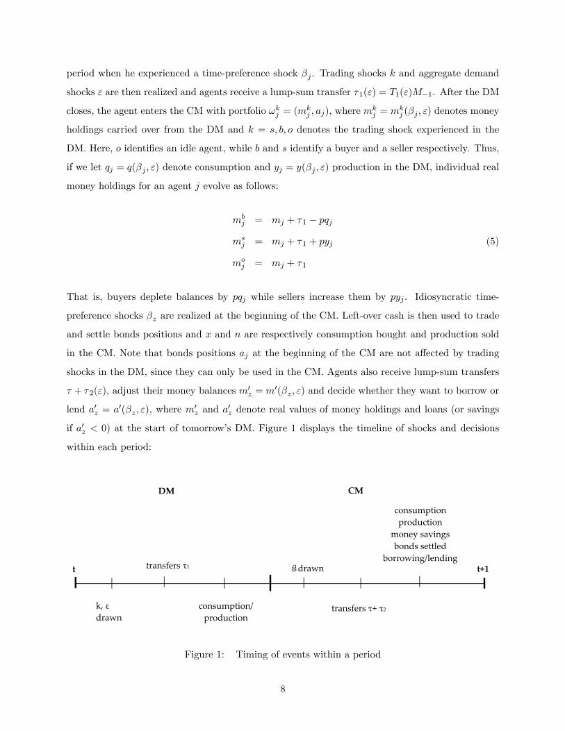
period when he experienced a time-preference shock βj . Trading shocks k and aggregate demand

shocks ε are then realized and agents receive a lump-sum transfer τ1(ε) = T1(ε)M−1. After the DM

closes, the agent enters the CM with portfolio ωkj = (mkj , aj), where m

kj = mk

j (βj , ε) denotes money

holdings carried over from the DM and k = s, b, o denotes the trading shock experienced in the

DM. Here, o identifies an idle agent, while b and s identify a buyer and a seller respectively. Thus,

if we let qj = q(βj , ε) denote consumption and yj = y(βj , ε) production in the DM, individual real

money holdings for an agent j evolve as follows:

mbj = mj + τ1 − pqj

msj = mj + τ1 + pyj (5)

moj = mj + τ1

That is, buyers deplete balances by pqj while sellers increase them by pyj . Idiosyncratic time-

preference shocks βz are realized at the beginning of the CM. Left-over cash is then used to trade

and settle bonds positions and x and n are respectively consumption bought and production sold

in the CM. Note that bonds positions aj at the beginning of the CM are not affected by trading

shocks in the DM, since they can only be used in the CM. Agents also receive lump-sum transfers

τ + τ2(ε), adjust their money balances m′z = m′(βz, ε) and decide whether they want to borrow or

lend a′z = a′(βz, ε), where m′z and a

′z denote real values of money holdings and loans (or savings

if a′z < 0) at the start of tomorrow’s DM. Figure 1 displays the timeline of shocks and decisions

within each period:

DM CM

k, ε drawn

consumption/ production

ßdrawn

transfers τ+ τ2

consumption production

money savings bonds settled

borrowing/lending t t+1transfers τ1

Figure 1: Timing of events within a period

8

Since we focus on stationary equilibria where end-of-period real money balances are time and

state invariant so that M/p2 = M ′/p′2, we have that

p′2p2

=M ′

M= π, (6)

which implies the inflation rate equals the growth rate of money supply. The government budget

constraint therefore is:

τ = (π − 1)[ρmH + (1− ρ)mL] (7)

Note that the long-run inflation rate is deterministic since the per capita lump-sum transfers τ in

the CM are not state dependent.

4.1 The CM problem

Given the recursive nature of the problem, we use dynamic programming to analyze the problem

of an agent j at any date, with j = H,L. We let V (ωj) denote the expected lifetime utility for an

agent entering the DM with portfolio ωj before shocks are realized. We also let Wz(ωkj ) denote the

expected lifetime utility from entering the CM with portfolio ωkj and receiving a discount factor

shock βz at the beginning of the CM.

The agent’s problem at the start of the CM then is:

Wz(ωkj ) = Max

xkjz ,nkjz ,a′z ,m′z

U(xkjz)− nkjz + βzV (ω′z)

s.t. xkjz + πm′z = nkjz +mkj + paπa

′z − aj + τ + τ2

s.t. a′z ≤ A (8)

s.t. m′z ≥ 0

where A ≥ 0 is a constant denoting an exogenous borrowing constraint. The resources available to

the agent in the CM depend on the realization of the DM trading shock k, as well as the aggregate

and idiosyncratic shocks ε, βj and βz. Specifically, an agent has mkj real balances carried over

from the DM and is able to borrow πa′z (or lend if a′z < 0) at a price pa. Other resources are nkjz

receipts from current sales of goods and lump-sum transfers τ + τ2. These resources can be used to

finance current consumption xj , to pay back loans aj and to carry πm′z real money balances into

9

next period. The factor π = p′2/p2 multiplies a′z and m′z because the budget constraint is expressed

in real terms.

Rewriting the constraint in terms of nkjz and substituting into (8) yields:

Wz(ωkj ) = Max

xkjz ,a′z ,m′z

U(xkjz)− xkjz − πm′z + πpaa′z − aj +mk

j + τ + τ2 + βzV (ω′z)

s.t. a′z ≤ A

s.t. m′z ≥ 0

Note that here we are focusing on a stationary equilibrium in which all agents provide a positive

labor effort. Conditions for nkjz > 0 are in the Appendix, but the intuition is that agents will always

choose to work in the CM if the borrowing limit A is tight enough. It follows that in a stationary

monetary economy we must have:

1 =∂Wz(ω

kj )

∂mkj

= −∂Wz(ω

kj )

∂aj(9)

This result depends on the quasi linearity of the CM preferences and the use of competitive pricing.

It implies that the marginal valuation of real balances and bonds in the CM are identical and do

not depend on the agent’s current type z or past type j, wealth ωkj or trade shock. This allows us

to disentangle the agents’portfolio choices from their trading histories since

Wz(ωkj ) = Wz(0) +mk

j − aj ,

i.e. the agent’s expected value from having a portfolio ωkj at the start of a CM is the expected value

from having no wealth, Wz(0), letting ωj = (0, 0) ≡ 0, plus the current real value of net wealth

mkj − aj . Note also that everyone consumes identically in the CM since:

U ′(x) = 1 (10)

which also implies x = x∗. That is, everyone consumes the same amount x∗ independent of current

type and past shocks, the reason being that agents in the CM can produce any amount at constant

marginal cost. Thus, goods market clearing in the CM requires:

x∗ = αbNb + αsN

s + (1− αb − αs)No (11)

10

where Nk = ρ2nkHH+ρ(1−ρ)(nkLH+nkHL)+(1−ρ)2nkLL is labor effort for all agents who experienced

a trading shock in the DM, with k = b, s, o. Let µmz ≥ 0 denote the Kuhn-Tucker multipliers

associated with the non-negativity constraint for money. Also, let λaz denote the multiplier on the

borrowing constraint. The first order conditions for the optimal portfolio choice then are:

1 =βzπ

∂V (ω′z)

∂m′z+ µmz /π (12)

−pa =βzπ

∂V (ω′z)

∂a′z− λaz/π (13)

The left hand sides of the expressions above define the marginal cost of the assets. The right hand

sides define the expected marginal benefit from holding the asset, either money or bonds, discounted

according to time preferences and inflation. From (12) and (13) we know that money holdings m′z

and bonds a′z are independent of trading histories and past demand shocks, but instead depend

on the current type z and the expected marginal benefit of holding money and bonds in the DM,

which may differ across types. We will study this next.

4.2 The DM problem

An agent with a portfolio ωj at the opening of the DM before aggregate demand and trading shocks

are realized has expected lifetime utility:

V (ωj) =

∫Ω

αbV

b(ωj) + αsVs(ωj) + (1− αb − αs)V o(ωj)

f(ε)dε (14)

First, we determine yj . The seller’s problem depends on the current disutility of production

and the expected continuation value. Specifically, the seller’s problem can be written as:

V s(ωj) = Maxyj

− c(yj) + ρWH(ωsj) + (1− ρ)WL(ωsj), (15)

for which the first order conditions, together with (5) and (9), give:

c′(yj) = p (16)

Note that (16) implies production is not type dependent, i.e. yj = y for j = H,L.

11

Now, we determine qj . A buyer’s problem is:

V b(ωj) = Maxqj

εu(qj) + ρWH(ωbj) + (1− ρ)WL(ωbj) (17)

s.t. pqj ≤ mj + τ1

The budget constraint reflects that consumption can be financed with both money holdings and

DM transfers. Let λbj denote the multiplier on the buyer’s budget constraint. Using (5) and (9),

the first order conditions for the buyer’s problem imply:

εu′(qj) = p(1 + λbj) (18)

From (16) and (18) we know that if the buyer is constrained and λbj > 0, then εu′[qj(ε)] > c′[y(ε)].

If instead the buyer is unconstrained and therefore λbj = 0, then εu′(qj(ε)) = c′(y(ε)).

Last, an idle agent’s problem is simply:

V o(ωj) = ρWH(ωnj ) + (1− ρ)WL(ωnj )

Goods market clearing therefore requires:

αsy(ε) = αb[ρqH(ε) + (1− ρ)qL(ε)] for ε ∈ Ω (19)

4.3 Monetary equilibrium

To find optimal savings for an agent j use (8), (14), (15), (16) and (17) to obtain:

V (ωj) =

∫Ω

mj − aj + τ1 + αb[εu(qj)− pqj ]− αs[c(y)− py] + EW (0)

f(ε)dε

The expected lifetime utility V (ωj) therefore depends on the agent’s net wealth and income mj −

aj +τ1 and two other elements: the expected continuation payoffEW (0) = ρWL(0)+(1−ρ)WL(0)

and the expected surplus from trade in the DM. With probability αb the agent spends pqj on

consumption deriving utility εu(qj) and with probability αs, instead, he gets disutility c(y) from

production and earns py from his sales. Note that, unlike in the representative-agent case, the

expected earnings p(y − qj) from DM trades might be different from zero since amounts produced

12

and consumed by an agent j = H,L may be mismatched. Hence, we have:

∂V (ωj)

∂mj=

∫Ω

1 + αb

[εu′(qj)

p− 1

]f(ε)dε (20)

and∂V (ωj)

∂aj= −1, (21)

which imply money is valued dissimilarly by agents, whereas bonds are valued identically in the

economy. Combining (12) with (20) and (13) with (21) one gets that in a monetary equilibrium

the following Euler equations must hold:

π − βjβj

=

∫Ω

αb

[εu′(qj(ε))

c′(y(ε))− 1

]f(ε)dε (22)

and

πpa = βz + λaz (23)

The expression in (22) tells us that the choice of real balances depends on three components. The

first two are standard: the discount factor βj at the beginning of the period and the real yield on

cash 1/π. The third component is εu′(qj)/c′(y). This can be interpreted as the expected liquidity

premium from having cash available in the DM and it arises because money is needed to trade

in that market. This premium grows with the severity of the cash constraint and the likelihood

of a consumption shock αb. The expression in (23), instead, refers to the choice of bonds, which

depends on the discount factor βz drawn at the beginning of the CM and the real yield 1/πpa.

Note that (23) implies that bonds have no liquidity premium. That is because they are always held

until maturity and cannot be used to buy consumption in the DM.

We can now define the equilibrium as the set of values of mj and az for j, z = H,L that solve

(22) and (23). The reason is that once the equilibrium stocks of money and bonds are determined,

all other endogenous variables can be derived.

Definition 1 A symmetric stationary monetary equilibrium consists of a mj satisfying (22) and

az satisfying (23) for j, z = H,L.

We now want to investigate whether a CM to CM bond az for z = H,L would indeed circulate

in this economy. We find that the following result holds:

Lemma 1 A stationary monetary equilibrium exists with impatient agents borrowing and patient

13

agents lending at a price pa = βH/π. Specifically, aL = A and aH = −(1− ρ)A/ρ.

Why are agents interested in trading such a bond in equilibrium? This is somewhat puzzling

since we know from (10) they always consume the effi cient quantity x∗ in the CM. This in turn

implies that there is no reason for using bonds for consumption smoothing here due to the quasi

linearity of preferences. Bonds, however, allow agents to smooth the labor effort across periods -

H agents prefer to work more today and less in the future, whereas L agents would rather do the

opposite.10

Once we know the price at which these bonds circulate in equilibrium, we can pin down their

net nominal yield, which is:

i =1

pa− 1 ⇒ i =

π

βH− 1 (24)

We will refer to i as the nominal interest rate in this economy - note it is affected directly by

long-term monetary policy through π. We now want to determine the returns on money and bonds

that are consistent with equilibrium.

Lemma 2 Any stationary monetary equilibrium must be such that π ≥ βH , i.e. i ≥ 0.

This result derives from a simple no-arbitrage condition - in a monetary equilibrium, the value

of money cannot grow too fast with π < βH or else type H agents will not spend it.11 This,

together with (24), implies that to run the Friedman rule the monetary authority must let π → βH

and cannot target βL instead.

5 Optimal inflation rate

At this point, we know that given the result in Lemma 2 the monetary authority is constrained

in its ability to give a rate of return on money that is attractive for everyone. Given this result,

one should expect ineffi ciencies will arise at i = 012 and therefore the Friedman rule might not be

the optimal policy here. We investigate this next, and in this section we will focus on the optimal

inflation rate in an economy without aggregate demand shocks, which we will then reintroduce in

Section 6. We find that the following result holds:10See Boel and Finocchiaro (2015) for an economy with borrowing and lending, where such a bond is traded even

with permanent heterogeneity in discounting.11Other models with heterogeneous time preferences have analogous results, in that the rate of return on the asset

cannot exceed the lowest rate of time preference. See for example Becker (1980) and Boel and Camera (2006). Inthose models, however, types are fixed.

12We know from (24) that it is equivalent to fix i or π.

14

Proposition 1 Let i = 0. If c′′(y) = 0, then qH = q∗ and qL < q∗. If c′′(y) > 0, then qH > q∗ and

qL < q∗.

Proposition 1 implies that, since agents value future consumption differently, the Friedman rule

fails to sustain the constrained-effi cient allocation in a monetary equilibrium. Indeed, even if the

Friedman rule eliminates the opportunity cost of holding money for type H agents, it still fails to

provide incentives for everyone to save enough since π > βL. That is because impatient agents

are facing an effective nominal interest rate equal to βH/βL − 1, which is positive. We know from

Lemma 2 that π ≥ βH and therefore the central bank is limited in its ability to reduce interest

rates even further. Thus, type L agents remain constrained even at the ZLB.

Proposition 1 also implies that the nature of preferences has important consequences for the

optimality of the Friedman rule. Specifically, a convex disutility from labor generates a price

externality induced by type L agents. This happens because impatient agents consume too little

even at π = βH , and therefore they drive down total output, marginal cost of production and

relative price. The low price in turn induces type H agents to consume too much compared to

the effi cient allocation. This price externality disappears with linear costs, since in that case the

marginal cost of production (and hence the relative price in the DM) is constant at any level of

output.

In light of the results described in Proposition 1, one must wonder if setting i = 0 is still the

optimal monetary policy in this economy. The following result clarifies when this is the case.

Proposition 2 If c′′(y) = 0, i = 0 is always the optimal policy. If c′′(y) > 0, i = 0 is the optimal

policy if c′(y) ≥ 1 and βLu′(qL) < βHu

′(qH).

The lesson here is that the Friedman rule is always the optimal policy with linear costs. In

that case, even if i = 0 fails to sustain the constrained-effi cient allocation, such policy delivers a

second best allocation that cannot be Pareto improved. With convex costs, however, the Friedman

rule is not necessarily optimal. Why not? Because the policy maker needs to take into account

the price externality induced by the underconsumption of impatient agents. In this situation,

Proposition 2 implies that i = 0 is optimal if two conditions hold. First, p = c′(y) ≥ 1, so that the

relative price cannot be too low in order to limit the overconsumption of type H agents. Second,

u′(qL)/u′(qH) < βH/βL, meaning the disparity in consumption between impatient and patient

agents must be limited.

15

Example 1 - optimal inflation with convex costs. In order to derive intuition for the results

in Proposition 2, we consider an example with the following functional forms:

u(q) = 1− exp−q and c(y) = expy −1

In this case, the optimal inflation problem to be solved in a monetary equilibrium becomes:

Maxπ

αb [(1− ρ)εu(qL) + ρεu(qH)]− αsc(y)

s.t.π − βHβH

= αb

[ε exp−qH

expy− 1

](25)

s.t.π − βLβL

= αb

[ε exp−qL

expy− 1

]s.t. αsy = αb[ρqH + (1− ρ)qL]

If we differentiate the objective function in (25), we find that the optimal π must satisfy:

αb

[(1− ρ)εu′(qL)

dqLdπ

+ ρεu′(qH)dqHdπ

]− αsc′(y)

[ρdqHdπ

+ (1− ρ)dqLdπ

]≤ 0 (26)

In the Appendix, we derive expressions for dqL/dπ and dqH/dπ from the constraint in (26) and let

ε = exp so that ln(ε) = 1. We find that in order for π = βH to be optimal in this case it must be

that:βH − βLβH

≤ αsρ(1− αb)

Intuitively, the condition above imposes an upper bound on time-preference heterogeneity. This

will limit the price externality highlighted in Propositions 1 and 2, and the Friedman rule will

be optimal with convex costs. Of course, if the condition above is not satisfied, then i > 0 must

be optimal. That would be the case, for example, with ρ = 0.90, βH = 0.99, βL = 0.70 and

αs = αb = 0.10. In this case the central bank would choose i = 1.46%.

6 Optimal stabilization policy at the ZLB

We now reintroduce aggregate demand shocks ε. We will first investigate which ineffi ciencies arise

when the central bank does not engage in stabilization policy, i.e. when τ1(ε) = τ2(ε) = 0. We will

call this passive policy and then compare it to active stabilization policy, i.e. the policy implemented

by a central bank whose objective is to maximize the weighted welfare of the agents in the economy.

16

We will do so for i = 0. We find the following result holds with passive policy.

Proposition 3 Let i = 0 and τ1(ε) = τ2(ε) = 0. A unique monetary equilibrium exists for

c′′(y) ≥ 0 such that: with c′′(y) = 0, then qL(ε) = qH(ε) = q∗(ε) for ε ≤ ε and qL(ε) < qH(ε) =

q∗(ε) for ε > ε, where ε ∈ [0, ε]; with c′′(y) > 0, then qL(ε) = qH(ε) = q∗(ε) for ε ≤ ε and

qL(ε) < q∗(ε) < qH(ε) for ε > ε, where ε ∈ [0, ε].

Proposition 3 implies that, with passive policy, impatient agents are unconstrained and consume

qL(ε) = q∗(ε) in low marginal demand states. They are instead constrained in high demand states,

and thus consume qL(ε) < q∗(ε). Why don’t type L ever consume qL(ε) > q∗(ε)? Because the price

externality outlined in Proposition 1 cannot arise when all agents are unconstrained, and therefore

qL(ε) = qH(ε) = q∗(ε) with c′′(y) ≥ 0 in the low marginal demand states. Agents will use the extra

cash to work less in the CM. Type H agents, instead, are never constrained, and they overconsume

only in high demand states with c′′(y) > 0.

We will now move to studying the problem of a central bank engaged in stabilization policy and

thus maximizing welfare by choosing the quantities consumed and produced by each type j = H,L

in each state subject to the constraint that the chosen quantities satisfy the conditions characterizing

a competitive equilibrium. The policy is then implemented by choosing state-contingent injections

τ1(ε) and τ2(ε) accordingly. The primal Ramsey problem faced by the central bank is:13

MaxqL(ε),qH(ε),y(ε)

∫Ωαbε [ρu(qH(ε)) + (1− ρ)u (qL(ε))]− αsc(y(ε)) f(ε)dε

s.t.π − βHβH

=

∫Ω

αb

[εu′(qH(ε))

c′(y(ε))− 1

]f(ε)dε

s.t.π − βLβL

=

∫Ω

αb

[εu′(qL(ε))

c′(y(ε))− 1

]f(ε)dε

s.t. αsy(ε) = αb[ρqH(ε) + (1− ρ)qL(ε)]

Note that we are focusing on a monetary equilibrium such that mj > 0 for j = H,L. That is why

the first two constraints in the Ramsey problem must hold with equality. Moreover, since i = 0,

then (22) implies that εu′(qH(ε)) = c′(y(ε)) in every state, and the Ramsey planner simply solves

13The objective function of the Ramsey problem faced by the central bank is:

ρ(1− βH)V (ωH) + (1− ρ)(1− βL)V (ωL)

where V (ωj) is defined in (14). We know that trades are effi cient in the CM. Moreover, τ1(ε) +τ2(ε) = 0 and m = ρmH + (1 − ρ)mL. Therefore, the central bank has to worry only about maximizing∫

Ωαbε [ρu(qH(ε)) + (1− ρ)u (qL(ε))] − αsc(y(ε)) f(ε)dε.

17

the following problem:

MaxqL(ε),y(ε)

∫Ωαbε [ρu(qH(ε)) + (1− ρ)u (qL(ε))]− αsc(y(ε)) f(ε)dε

s.t.π − βLβL

=

∫Ω

αb

[εu′(qL(ε))

c′(y(ε))− 1

]f(ε)dε (27)

s.t. αsy(ε) = αb[ρqH(ε) + (1− ρ)qL(ε)]

We find the following result holds:

Proposition 4 If i = 0, in a monetary equilibrium with mj > 0 for j = H,L the optimal policy is

qL(ε) < q∗(ε) for all states with c′′(y) ≥ 0.

Why does the Ramsey planner choose qL < q∗ in all states? Because we know from Proposition

3 that without policy intervention agents L would have enough cash to buy q∗ in low demand states.

In high demand states, however, their cash holdings would constrain their spending to qL < q∗.

This would create an ineffi ciency of consumption across states that can be overcome by stabilization

policy.

It is worth emphasizing that our aim here is to determine how stabilization policy can improve

welfare compared to the allocation that would be achieved with a passive policy in which agents

would only be able to rely on their money balances to finance consumption in the DM. That is why

Proposition 4 focuses on an equilibrium where mj(ε) > 0 for j = H,L. Of course the central bank

could also provide L agents with enough liquidity to finance q∗(ε) in every state, but in that case

we would have mL(ε) = 0 in all states since L agents would have no incentive to bring any money.

Note that Proposition 4 also implies that the central bank is able to temporarily relax liquidity

constraints on impatient agents at the ZLB. It can do so simply engaging in repo arrangements

that are undone at a later date, i.e. τ1(ε) + τ2(ε) = 0.

Example 2 - stabilization policy with linear costs. We now want to get some intuition about

optimal stabilization policy at the zero lower bound with different cost functions specifications. We

will focus on linear costs first, and specifically we consider the following functional forms:

u(q) = 1− exp−q and c(y) = y

18

Derivations are in the Appendix, but it is worth pointing out that in this case we find that:

qL(ε) = ln(ε)− ln

[π − βL(1− αb)

αbβL

]

and qL(ε)/qL(ε) can be expressed as:

ln(ε)− ln [(π − βL(1− αb))/αbβL]

ln(ε)− ln [(π − βL(1− αb))/αbβL]=mL + τ1(ε)m/π

mL + τ1(ε)m/π

Since ε > ε, then it must be that τ1(ε) > τ1(ε). Thus, the higher the demand for good, the higher

the injection τ1(ε) needed to finance the increase in consumption.

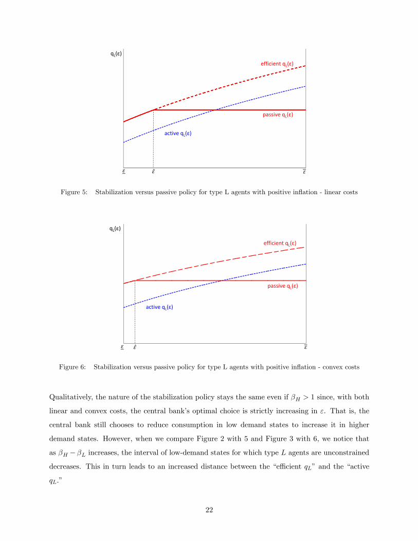
Figure 2 illustrates active and passive policies for type L with the specified linear cost function

and assuming the following parameter values: αs = αb = 0.3, βH = 0.99, βH = 0.95, ρ = 0.5. The

values for βH and βL are consistent with the evidence in Lawrence (1991), Carroll and Samwick

(1997) and Samwick (1998) who provide empirical estimates of distributions of discount factors.

The curve labeled “effi cient qL(ε)”represents the constrained-effi cient allocation at which q∗(ε) =

q∗H(ε) = q∗L(ε). The curve “passive qL(ε)”represents equilibrium consumption for type L under a

passive policy, whereas the curve “active qL(ε)”denotes consumption for the same agents when the

central bank behaves optimally.

The important thing to notice here is that the central bank’s optimal choice is strictly increasing

in ε - the central bank chooses to reduce consumption from the first best in low demand states in

order to increase it in higher demand states.

qL(ε)

efficient qL(ε)

passive qL(ε)

active qL(ε)

Figure 2: Stabilization versus passive policy for type L agents - linear costs

19

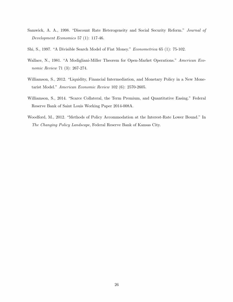
Example 3 - stabilization policy with convex costs. In this example, we focus on convex

costs and consider the following functional forms:

u(q) = 1− exp−q and c(y) = expy −1

Derivations are in the Appendix. Figure 3 illustrates active and passive policies for type L in this

example using the same parameter values we used for the linear cost function specification. As in

that case, the central bank’s optimal choice is strictly increasing in ε - the central bank chooses to

reduce consumption from the first best in low demand states to increase it in higher demand states.

qL(ε)

efficient qL(ε)

passive qL(ε)

active qL(ε)

Figure 3: Stabilization versus passive policy for type L agents - convex costs

Note that the central bank is not actively trying to stabilize consumption of patient agents. How-

ever, the short-term monetary policy aimed at stabilizing qL(ε) generates an externality on qH(ε).

Figure 4 illustrates. The important thing to notice here is that since qL < q∗ in all states, type

H agents always consume more than q∗ in light of Proposition 1. We know from Proposition 3

that without policy intervention agents H would buy q∗ in some states and qH > q∗ in others.

Stabilization policy addresses this discontinuity indirectly and consumption is smoothed so that

qH > q∗ in all states.

20

qH(ε)

efficient qH(ε)

passive qH(ε)

active qH(ε)

Figure 4: Stabilization versus passive policy for type H agents - convex costs

6.1 Optimal stabilization policy with positive inflation at the ZLB

We now consider the following scenario. We are at the steady state and right before the CM opens

the spread between βH and βL unexpectedly widens for only one period. Specifically, we consider

the case 0 < βL < β < 1 < βH for one period, but 0 < βL < β < βH < 1 from then on with

average β invariant. Note that, given Lemma 2, a discount factor βH > 1 implies a positive inflation

rate at the zero lower bound, and therefore a negative real interest rate. Note also that, with this

particular structure, transversality conditions still hold for H agents in the CM in period t since

their expected discount factor is lower than one after that, i.e. β < 1.14 The analytical results

derived in the previous sections still hold even if the spread between the discount factors widens.

Quantitatively, however, results do change since from (22) we have:

dqjdβj

= − π[c′(y)]2

β2jαbε[u

′′(qj)c′(y)− u′(qj)c′′(y)dy/dqj ]

and therefore dqj/dβj > 0. Thus, as βL decreases, impatient agents will become more constrained

at the ZLB. We therefore investigate how the results from the Ramsey problem in this environment

compare to the ones where the spread is narrower. For our numerical analysis, we consider βH =

1.005 (consistent with an annual 2% inflation) and βL = 0.935, so that β = 0.970 as in our previous

exercises. All other parameters and functional forms remain invariant. Figures 5 and 6 illustrate

the results for impatient agents for the cases of linear and convex disutility respectively.

14See Kocherlakota (1990) for a related discussion in the context of growth economies.

21

qL(ε)

efficient qL(ε)

passive qL(ε)

active qL(ε)

Figure 5: Stabilization versus passive policy for type L agents with positive inflation - linear costs

qL(ε)

efficient qL(ε)

passive qL(ε)

active qL(ε)

Figure 6: Stabilization versus passive policy for type L agents with positive inflation - convex costs

Qualitatively, the nature of the stabilization policy stays the same even if βH > 1 since, with both

linear and convex costs, the central bank’s optimal choice is strictly increasing in ε. That is, the

central bank still chooses to reduce consumption in low demand states to increase it in higher

demand states. However, when we compare Figure 2 with 5 and Figure 3 with 6, we notice that

as βH − βL increases, the interval of low-demand states for which type L agents are unconstrained

decreases. This in turn leads to an increased distance between the “effi cient qL”and the “active

qL.”

22

7 Conclusion

There is substantial empirical evidence showing that QE can have beneficial real effects on the

economy even at the ZLB. Yet, at the same time, showing theoretically that QE can be welfare

improving has been diffi cult to achieve. Our study is motivated by the desire to reconcile these

observations. For this reason, we construct a New Monetarist model characterized by aggregate and

idiosyncratic demand shocks. Agents are heterogeneous with respect to the idiosyncratic shock,

so that in every period some agents are more patient than others. This heterogeneity generates a

distribution in asset holdings. We then study the optimal stabilization response of the central bank

to demand shocks that hit the economy.

We find that several results hold in this environment. First, the ZLB can be the best interest

rate policy the central bank can implement although that is not necessarily the case due to a

price externality. However, even when the ZLB is the best policy, not all agents are satiated

at the Friedman rule and therefore there is scope for central bank policies of liquidity provision.

Second, we study a particular form of QE whereby the central bank purchases private debt via

repo arrangements in response to demand shocks. We find that such a policy is welfare improving

even at the ZLB since it can relax the liquidity constraint of impatient agents without harming the

patient ones. We show this is true regardless of whether we have inflation or deflation at the ZLB.

Third, due to a pricing externality, QE can be welfare improving for patient agents even if they are

unconstrained at the ZLB.

23

References

Akyol, A., 2004. “Optimal Monetary Policy in an Economy with Incomplete Markets and Idiosyn-

cratic Risk.”Journal of Monetary Economics 51 (6): 1245-1269.

Becker, R., 1980. “On the Long-Run Steady State in a Simple Dynamic Model of Equilibrium with

Heterogeneous Households.”Quarterly Journal of Economics 95 (2): 375-382.

Berentsen, A., Camera, G., and C. J. Waller, 2007. “Money, Credit and Banking.” Journal of

Economic Theory 135 (1): 171-195.

Berentsen, A., and C. J. Waller, 2011. “Price-Level Targeting and Stabilization Policy.”Journal of

Money, Credit and Banking 43 (7): 559-580.

Berentsen, A., Huber, S., and A. Marchesiani, 2014. “Degreasing the Wheels of Finance.”Interna-

tional Economic Review, 55 (3): 735-763.

Bhattacharya, J., Haslag, J., and A. Martin, 2005. “Heterogeneity, Redistribution, and the Fried-

man Rule.”International Economic Review 46 (2): 437-454.

Bhattarai, S., Eggertsson, G.B., and B. Gafarov, 2015. “Time Consistency and the Duration of

Government Debt: a Signalling Theory of Quantitative Easing.”NBER Working Paper 21336.

Boel, P., and G. Camera, 2006. “Effi cient Monetary Allocations and the Illiquidity of Bonds.”

Journal of Monetary Economics 53 (7): 1693-1715.

Boel, P., and D. Finocchiaro, 2015. “Money, Credit and Redistribution.”Unpublished Manuscript,

Sveriges Riksbank.

Carroll, C. D., and A. A. Samwick, 1997. “The Nature of Precautionary Wealth.” Journal of

Monetary Economics 40 (1): 41-71.

Cúrdia, V., and M. Woodford, 2011. “The Central-Bank Balance Sheet as an Instrument of Mon-

etary Policy.”Journal of Monetary Economics 58 (1): 47-74.

Eggertsson, G. B., and M. Woodford, 2003. “The Zero Bound on Interest Rates and Optimal

Monetary Policy.”Brookings Papers on Economic Activity, Vol. 1: 139-211.

Eggertsson, G. P., and P. Krugman, 2012. “Debt, Deleveraging, and the Liquidity Trap: a Fisher-

Minsky-Koo Approach.”Quarterly Journal of Economics 127 (3): 1469-1513.

24

Gagnon, J., Raskin, M., Remache, J., and B. Sack, 2010. “Large-Scale Asset Purchases by the

Federal Reserve: Did They Work?” Federal Reserve Bank of New York Staff Report no. 441

(March).

Hamilton, J. D., and J. C. Wu, 2012. “The Effectiveness of Alternative Monetary Policy Tools in

a Zero Lower Bound Environment.”Journal of Money, Credit and Banking 44 (1): 3-46.

Herrenbrueck, L., 2014. “Quantitative Easing and the Liquidity Channel of Monetary Policy.”

Simon Fraser University Working Paper.

Ireland, P. N., 2005. “Heterogeneity and Redistribution: by Monetary or Fiscal Means?” Interna-

tional Economic Review 46 (2): 455-463.

Kocherlakota, N., 1990. “On the Discount Factor in Growth Economies.” Journal of Monetary

Economics 25 (1): 43-47.

Kocherlakota, N., 1998. “Money is Memory.”Journal of Economic Theory 81 (2): 232-251.

Krishnamurthy, A., and A. Vissing-Jorgensen, 2011. “The Effects of Quantitative Easing on Interest

Rates: Channels and Implications for Policy.”Brookings Papers on Economic Activity, Vol. 2:

215-287.

Lagos, R., and R. Wright, 2005. “A Unified Framework for Monetary Theory and Policy Analysis.”

Journal of Political Economy 113 (3): 463-484.

Lawrence, E. C., 1991. “Poverty and the Rate of Time Preference: Evidence from Panel Data.”

Journal of Political Economy 99 (1): 54-77.

Phelps, E. S., 1973. “Inflation in the Theory of Public Finance.”Swedish Journal of Economics 75

(1): 67-82.

Ramsey, F. P., 1927. “A Contribution to the Theory of Taxation.” The Economic Journal 37:

47-61.

Rocheteau, G., and R. Wright, 2005. “Money in Search Equilibrium, in Competitive Equilibrium

and in Competitive Search Equilibrium.”Econometrica 73 (1): 175-202.

Rojas Breu, M., 2013. “The Welfare Effect of Access to Credit.”Economic Inquiry, 51 (1): 235-247.

25

Samwick, A. A., 1998. “Discount Rate Heterogeneity and Social Security Reform.” Journal of

Development Economics 57 (1): 117-46.

Shi, S., 1997. “A Divisible Search Model of Fiat Money.”Econometrica 65 (1): 75-102.

Wallace, N., 1981. “A Modigliani-Miller Theorem for Open-Market Operations.”American Eco-

nomic Review 71 (3): 267-274.

Williamson, S., 2012. “Liquidity, Financial Intermediation, and Monetary Policy in a New Mone-

tarist Model.”American Economic Review 102 (6): 2570-2605.

Williamson, S., 2014. “Scarce Collateral, the Term Premium, and Quantitative Easing.”Federal

Reserve Bank of Saint Louis Working Paper 2014-008A.

Woodford, M., 2012. “Methods of Policy Accommodation at the Interest-Rate Lower Bound.” In

The Changing Policy Landscape, Federal Reserve Bank of Kansas City.

26

8 Appendix

Conditions for nkjz > 0. We now want to provide conditions that guarantee nkj,z ≥ 0 in the

constrained-effi cient equilibrium with i = 0. Note that if nsHL > 0, then nkjz ≥ 0 in all other cases.

We know that xkjz = x∗ for all j, z. This, together with the budget constraint in (8), implies:

nsHL = x∗ −msH + πmL − πpaaL + aH − τ − τ2

From (5), Lemma 1 and (7) the expression above becomes:

nsHL = x∗ −mH − τ1 − py + βHmL −A[βH + (1− ρ)/ρ]− (βH − 1)(ρmH + (1− ρ)mL)− τ2

Since τ1 + τ2 = 0 and py = ρ(mH + τ1) + (1− ρ)(mL + τ1), rearranging we get:

nsHL = x∗ −A[βH + (1− ρ)/ρ]−mH − τ1 − ρβH [ρmH + (1− ρ)mL]

Note that for π = βH we have thatmH−τ1 = q∗. LetK = ρβH [ρmH+(1−ρ)mL]+A[βH+(1−ρ)/ρ].

Then, in order to have nsHL > 0 it must be that:

x∗ − q∗ > K (28)

Since K > 0, then x∗ must be suffi ciently bigger than q∗ in order to have nsHL > 0. Note that

the necessary difference between q∗ and x∗ will depend on A - a tighter borrowing constraint will

generate an incentive to work.

Proof of Lemma 1 From the Euler equation in (23) we have that the following must hold:

βL + λL = βH + λH

Since βH > βL, it must be that λL > λH ≥ 0. If λL > λH > 0, then there is no borrowing or

lending. If instead λL > λH = 0, then aL = A and given the bonds market clearing condition

ρaH + (1− ρ)aL = 0 (29)

we have that aH = −A(1− ρ)/ρ. Since πpa = βH from (23), then pa = π/βH .

27

Proof of Lemma 2 We know from (16) and (18) that εu′(qj) ≥ c′(y) for j = H,L. This, together

with (22), implies that π ≥ βH .

Proof of Proposition 1 From (22) and (18) we know that if π = βH then εu′(qL) > c′(y), thus

implying type L agents are constrained and qL < q∗ for c′′(y) ≥ 0. From (22) and (18) we also

know that if π = βH then εu′(qH) = c′(y), thus implying type H agents cannot be constrained and

qH ≥ q∗. Assume qH = q∗. Since qL < q∗, then we have that y < y∗ where y∗ = (αb/αs)q∗. With

c′′(y) = 0 this would imply εu′(q∗) = c′(y) = c′(y∗) since c′(y) is constant and therefore qH = q∗.

With c′′(y) > 0, instead, y < y∗ implies εu′(q∗) = c′(y) < c′(y∗). Therefore, it cannot be that

qH = q∗ and it must be qH > q∗.

Proof of Proposition 2 The optimal π maximizes

Maxπ

αb [(1− ρ)εu(qL) + ρεu(qH)]− αsc(y) (30)

subject to the constraints

s.t.π − βHβH

= αb

[εu′(qH)

c′(y)− 1

]s.t.

π − βLβL

= αb

[εu′(qL)

c′(y)− 1

](31)

and the DM market clearing condition (19). By differentiating the objective function in (30), we

know that in order for π = βH to be the optimal policy, the following condition must hold:

(1− ρ)[εu′(qL)− c′(y)

] dqLdπ

∣∣∣∣π=βH

+ ρ[εu′(qH)− c′(y)

] dqHdπ

∣∣∣∣π=βH

≤ 0 (32)

From the Euler equations we know that εu′(qH)−c′(y) = 0 and εu′(qL)−c′(y) > 0 at the Friedman

rule. Therefore, (32) becomes

(1− ρ)[εu′(qL)− c′(y)

] dqLdπ

∣∣∣∣π=βH

≤ 0,

which implies the Friedman rule will only be optimal if dqLdπ

∣∣∣π=βH

≤ 0. Now, if we totally differen-

tiate the constraints in (31), we find the following system of equations has to hold:

28

nεu′′(qH)

c′(y)− nεu

′(qH)c′′(y)

c′(y)2

n

sρ −nεu

′(qH)c′′(y)

c′(y)2

n

s(1− ρ)

−nεu′(qL)c′′(y)

c′(y)2

n

sρ n

εu′′(qL)

c′(y)− nεu

′(qL)c′′(y)

c′(y)2

n

s(1− ρ)

dqHdπ

dqLdπ

=

1

βH

1

βL

where the determinant D is

D =α2b

c′(y)2

[εu′′(qH)− κH

] [εu′′(qL)− κL

]− α2

b

c′(y)2κLκH

with κH = (αb/αs)ρεu′(qH)c′′(y)/c′(y) and κL = (αb/αs)(1− ρ)εu′(qL)c′′(y)/c′(y). Using Cramer’s

rule we have:

dqLdπ

=αb

c′(y)D

[εu′′(qH)− εu′(qH)c′′(y)

c′(y)

αbαsρ

]1

βL+

[εu′(qL)c′′(y)

c′(y)

αbαsρ

]1

βH

anddqLdπ

∣∣∣∣π=βH

=αb

c′(y)D

1

βL

εu′′(qH) +

[u′(qL)

u′(qH)

βLβH− 1

]c′′(y)

αbαsρ

Since

D|π=βH=

α2b

c′(y)[(εu′′(qH)− κH)(εu′′(qL)− κL)− α2

bκLαbαsρc′′(y)/c′(y)], (33)

then at π = βH it must be that

dqLdπ

=εu′′(qH) +

[u′(qL)u′(qH)

βLβH− 1]αbαsρc′′(y)

αbβL

[εu′′(qH)− c′′(y)αbαs ρ

] [εu′′(qL)− u′(qL)c′′(y)

u′(qH)αbαs

(1− ρ)]−[εu′(qL)c′(y)2

αbαsρ] [

αbαs

(1− ρ)]c′′(y)2

Note that if c′′(y) = 0 then dqL

dπ

∣∣∣π=βH

< 0, which implies the Friedman rule is always the optimal

policy with linear costs. If instead if c′′(y) > 0, then the sign of dqLdπ

∣∣∣π=βH

< 0 is indeterminate and

therefore the Friedman rule is not necessarily optimal. Note that (33) can be simplified as

D|π=βH= − α2

b

α2sc′(y)3

ε(u′(qL)α2bc′′(y)2ρ(1− ρ)

[1− c′(y)

]− α2

su′′(qH)c′(y)2u′′(qL)ε)

− α2b

α2sc′(y)3

εc′′(y)αsc′(y)ε

[u′(qL)u′′(qH)(1− ρ) + αbu

′(qH)u′′(qL)ρ]

Therefore, if c′′(y) > 0 then D|π=βH> 0 if and only if c′(y) ≥ 1. If c′(y) ≥ 1, then dqL

dπ

∣∣∣π=βH

< 0 if

u′(qL)/u′(qH) < βH/βL.

29

Proof of Proposition 3 From (22) we have:

π − βLβL

=

∫ ε

ε

αb

[εu′(qL(ε))

c′(y(ε))− 1

]f(ε)dε (34)

Let gL(ε) denote real aggregate spending of type L agents when their trades are effi cient, i.e.

gL(ε) = αb(1− ρ)p(ε)q∗(ε). Now we want to understand how changes in ε affect gL(ε):

dgL(ε) = αb(1− ρ) [q∗(ε)dp+ p(ε)dq∗]

The first term denotes the change in the relative price p(ε) and the second one changes in the

effi cient quantity q∗(ε). We can rewrite it as follows:

dgL(ε) = αb(1− ρ)pq∗[dp

p+dq∗

q∗

]

From (16) we derive that:

dp

p= 0

The term dq∗/q∗, instead, can be derived from εu′(q∗) = c′[(αb/αs)q∗]:

dq∗

q∗= − εu′(q∗)

εu′′(q∗)− c′′[(αb/αs)q∗](αb/αs)dε

ε

so that:dgL(ε)

dε= − αb(1− ρ)c′[(αb/αs)q

∗]q∗u′(q∗)

εu′′(q∗)− c′′[(αb/αs)q∗](αb/αs)> 0 for c′′(y) ≥ 0

Let’s first consider the case c′′(y) = 0. If gL(ε) > mL, then agents are constrained in all states. If

gL(ε) < mL, then agents are never constrained. If gL(ε) ≥ mL ≥ gL(ε), for a given value of mL

there exists a critical value ε such that gL(ε) = mL. This implies that qL(ε) = q∗(ε) = qH(ε) for

ε ≤ ε and qL(ε) < q∗(ε) = qH(ε) for ε > ε.

The RHS of (22) is a function ofmL. Note that limmL→0

RHS =∞ and, for mL = g(ε), RHS|mL=

0 ≤ (π − βL)/βL. Since RHS is continuous in mL then an equilibrium exists.

The RHS of (22) is monotonically decreasing in mL. To see this use Leibnitz’s rule and note

that by construction qL(ε) = q∗(ε) to get

∂RHS

∂mL=

∫ ε

ε

αb

[ε [u′′c′ − u′c′′(αb/αs)(1− ρ)]

(c′)2

∂qL∂mL

]f(ε)dε < 0

30

Since the right-hand side is strictly decreasing in mL, we have a unique mL that solves (34).

Consequently, we have qL(ε) = q∗(ε) if ε ≤ ε and qL(ε) < q∗(ε) otherwise.

The argument is analogous for the case c′′(y) > 0 and there exists a unique critical value ε such

that gL(ε) = mL. However, we know from Proposition 1 that when type L agents are constrained

type H ones consume more than q∗. This implies that qL(ε) = q∗(ε) = qH(ε) for ε ≤ ε and

qL(ε) < q∗(ε) < qH(ε) for ε > ε.

Proof of Proposition 4 The Lagrangian for (27) is:

L = MaxqL(ε),y(ε)

∫Ωαb(1− ρ)εu(qL(ε)) + αbρεu(qH(ε))− αsc (y(ε))f(ε)dε

+λR

[∫Ω

αb

[εu′(qL(ε))

c′ (y(ε))− 1

]f(ε)dε− π − βL

βL

]+ µ(ε)

[y(ε)− αb

αs(ρqH(ε) + (1− ρ)qL(ε))

]

Note that µ is a function of ε because the resource constraint varies state by state. The first order

condition with respect to qL(ε) and y(ε) are respectively as in (42) and (43). Note that, since

εu′(qH(ε)) = c′(y(ε)) at i = 0, from the implicit function theorem we know that

dqH(ε)

dy(ε)=

c′′ (y(ε))

εu′′(qH(ε))(35)

Therefore, combining (42), (43) and (35) we find that the following expression holds for c′′(y) ≥ 0 :

εu′(qL(ε))− c′ (y(ε)) =λR

(1− ρ) c′ (y(ε))2

αbεu′(qL(ε))c′′ (y(ε))− αbαsu′′(qL(ε))

αs − αbρc′′ (y(ε)) /εu′′(qH(ε))(36)

At this point we need to consider two cases. In the first one, mL > 0 and therefore (27) holds with

equality so that λR > 0. Therefore, εu′(qL(ε)) > c′ (y(ε)) in (36), which implies qL(ε) < q∗(ε). In

the second one, mL = 0 and therefore λR = 0. This in turn implies εu′(qL(ε)) = c′ (y(ε)) in (36),

so that qL(ε) = qH(ε) = q∗(ε).

31

Derivations for Example 1. We consider the following functional forms:

u(q) = 1− exp−q and c(y) = expy −1

In this case, the constraints in the optimal inflation problem become:

π − βHβH

= αb

[ε exp−qH

expy− 1

]π − βLβL

= αb

[ε exp−qL

expy− 1

](37)

αsy = αb[ρqH + (1− ρ)qL]

The derivative of the objective function with respect to π yields:

αbε

[(1− ρ)u′(qL)

dqLdπ

+ ρu′(qH)dqHdπ

]− αsc′(y)

[ρdqHdπ

+ (1− ρ)dqLdπ

]≤ 0 (38)

We now need to find expressions for dqL/dπ and dqH/dπ. If we simplify the expressions in the

constraints in (37) and take logs, we find that:

qH =αsZH + αb(1− ρ) (ZH − ZL)

αs + αb

qL =αsZL − αbρ (ZH − ZL)

αs + αb

where ZH = ln(ε) + ln [αbβH/(π − βH + αbβH)] and ZL = ln(ε) + ln [αbβL/(π − βL + αbβL)]. We

let ε = exp so that ln(ε) = 1. Then:

dqLdπ

=αbρ

(αs + αb) (π − βH + αbβH)− αs + αbρ

(αs + αb) (π − βL + αbβL)

anddqHdπ

=αb(1− ρ)

(αs + αb) (π − βL + αbβL)− αs + αb(1− ρ)

(αs + αb) (π − βH + αbβH)

By plugging the expressions for dqL/dπ and dqH/dπ into (38), we find that in order for π = βH to

be optimal it must be that (1−ρ) [− (αs + αbρ) (αbβH) + αbρ (βH − βL + αbβL)][exp1−ZL −1

]≤ 0.

Therefore, the following condition must hold:

βH − βLβH

≤ αsρ(1− αb)

32

Derivations for Example 2. In this example, we focus on linear costs and consider the following

functional forms:

u(q) = 1− exp−q and c(y) = y

The central bank’s problem is as in (27) and the first-order condition with respect to qL(ε) is:

(1− ρ)[εu′(qL(ε))− 1

]= −ελRu′′qL(ε),

thus implying

λR = −(1− ρ) [εu′(qL(ε))− 1]

εu′′(qL(ε))(39)

Note λR does not depend on any state ε and hence it must be:

(1− ρ) [εu′(qL(ε))− 1]

εu′′(qL(ε))=

(1− ρ) [εu′(qL(ε))− 1]

εu′′(qL(ε))

This, together with the specific functional forms we chose for this example, implies ln(ε)− ln(ε) =

qL(ε) − qL(ε). Hence, if ε > ε, we know that qL(ε) > qL(ε). Now, assume τ1(ε) = 0. Note that

when agents are constrained it must be that qL(ε) = mL + τ1(ε)m/π and therefore:

qL(ε) =

[mL + τ1(ε)m/π

mL + τ1(ε)m/π

]qL(ε)

With the specified functional forms (39) becomes λR = (1 − ρ)[ε exp−qL(ε)−1

]/ε exp−qL(ε) and

therefore ε exp−qL = 1− ρ/ [1− ρ− λ]. By taking logs of both hand sides, we find that:

qL(ε) = ln(ε)− ln

[1− ρ

(1− ρ)− λR

](40)

Note that with a linear cost function the constraint in (27) becomes:

π − βLβL

=

∫ ε

ε

αb[ε exp−qL −1]

f(ε)dε

If we combine it with (40) we have that (π − βL)/βL = αbλR/(1− ρ− λR) and therefore:

λR =(1− ρ)(π − βL)

π − βL + αbβL> 0 (41)

33

Thus, combining (40) with (41) we find that:

qL(ε) = ln(ε)− ln

[π − βL(1− αb)

αbβL

]

Since we know that qL(ε) = qL(ε) [mL + τ1(ε)m/π] / [mL + τ1(ε)m/π], then we have that:

ln(ε)− ln [(π − βL(1− αb))/αbβL]

ln(ε)− ln [(π − βL(1− αb))/αbβL]=mL + τ1(ε)m/π

mL + τ1(ε)m/π

Since ε > ε, then it must be that τ1(ε) > τ1(ε). Thus, the higher the demand for good, the higher

the injection τ1(ε) needed to finance the increase in consumption.

Derivations for Example 3. In this example, we focus on convex costs and consider the fol-

lowing functional forms:

u(q) = 1− exp−q and c(y) = expy −1

As before, the central bank’s problem is as in (27). The first-order condition for qL(ε) implies:

µ(ε) = εαs(1− ρ)u′(qL(ε)) + λRu

′′ [qL(ε)] /c′ (y(ε))

1− ρ (42)

The first order condition with respect to y(ε) instead yields:

αbρεu′(qH(ε))

dqH(ε)

dy(ε)− αsc′ (y(ε))− λR

αbεu′(qL(ε))c′′ (y(ε))

c′ (y(ε))2 + µ(ε)

[1− αb

αsρdqH(ε)

dy(ε)

]= 0 (43)

Combining (42) with (43) and the fact that with convex costs dqH(ε)/dy(ε) = c′′ [y(ε)] /εu′′ [qH(ε)]

and solving for λR, we find:

λR =

εu′ [qL(ε)]− c′[y(ε)]

[1− αb

αsρ

c′′[y(ε)]

εu′′ [qH(ε)]

]αbεu

′ [qL(ε)] c′′[y(ε)]

αsc′[y(ε)]2− εu′′ [qL(ε)]

(1− ρ)c′[y(ε)]

[1− αb

αsρ

c′′[y(ε)]

εu′′ [qH(ε)]

] (44)

We now consider a uniform distribution with ε = exp and we proceed as follows. First, we use the

first constraint in the Ramsey problem in (27) to solve for y(ε):

π − βLβL

=

∫ ε

ε

αbε exp

αbρ ln(ε)− (αs + αb)y(ε)

αb(1− ρ) −1

f(ε)dε

34

Second, since λR does not depend on any state ε, the following condition must hold for all ε such

that ε ≤ ε ≤ ε given an arbitrary state ε:

λR = λR|ε with λR =

[ε exp−qL(ε)− expy(ε)

] [1− αb

αsρ

expy(ε)

−ε expqH(ε)

]αbε exp−qL(ε) expy(ε)

αs[expy(ε)]2− −ε exp−qL(ε)

(1− ρ) expy(ε)

[1− αb

αsρ

expy(ε)

−ε expqH(ε)

]

We use this to solve for y(ε) in terms of y(ε) for all ε. Then, we use the resource constraint (19) to

solve for qL(ε) as a function of y(ε):

qL(ε) =y(ε)(αs + αbρ)− αbρ ln(ε)

αb(1− ρ)

Last, from εu′ [qH(ε)] = c′[y(ε)] we find an expression for qH(ε) as a function of y(ε). With the

functional forms we chose, the condition is qH(ε) = ln(ε)− y(ε).

35