on the theory of electromagnetic induction in the earth · pdf fileon the theory of...

JOURNAL OF GEOPHYSICAL RESEARCH, VOL. 88, NO. B4, PAGES 3531-3542, APRIL 10, 1983

On the Theory of Electromagnetic Induction in the Earth by Ocean Currents

ALAN D. CHAVE

Institute of Geophysics and Planetary Physics, Scripps Institution of Oceanography University of California at San Diego, La Jolla California 92093

The theory of electromagnetic induction is extended to the case where the driving electric currents must be considered explicitly. Differential equations for independent poloidal magnetic (PM) and toroidal magnetic (TM) modes are derived directly from the governing quasistatic form of the Maxwell equations. They are applied to induction by motional source fields in the ocean by deriving Green functions for the two modes in a constant depth ocean. PM and TM modes are shown to behave in very different ways as a function both of the ocean velocity field dynamics and of the electrical conductivity structure of the earth. TM modes are closely associated with the Coriolis force deflection of water currents and with coastline effects that limit the source currents to the ocean basin. PM modes are induced by nondivergent electric currents that are fully contained within the ocean. Surface gravity waves and a Kelvin wave are examined in detail. The Kelvin wave result of Larsen (1968) is reevaluated, and because the upper lithosphere was modeled as an insulator, significant errors in his magnetic induction values, caused by neglect of the TM mode, are revealed. The sensitivity of the TM mode magnetic field to lithospheric electrical conductivity suggests the use of tidal induced electromagnetic fields to probe the earth's conductivity structure.

INTRODUCTION

Electromagnetic fields are induced in the earth by external, ionospheric and magnetospheric, current systems and have long been used to investigate the electrical conductivity structure of the earth by the geomagnetic depth sounding or magnetotelluric methods. An additional natural source, the dynamo interaction of ocean currents with the ambient geomagnetic field, is important in the world oceans. Since the crust and mantle of the earth are

electrical conductors that couple to the ocean both conduc- tively and inductively, observations of low-frequency electromagnetic fields in the ocean contain information about both the electrical conductivity of the earth and the circu- lation of the oceans.

Electromagnetic fields produced by ocean flows are discussed by Cox et al. [1971], Sanford [1971], and Larsen [1973]. Solutions of the Maxwell equations for surface gravity waves were obtained by Weaver [1965] for an infinitely deep ocean and were extended to long waves in a finite depth ocean by Larsen [1971]. The surface and internal wave problem was also investigated by Podney [1975], who presented a general method for solving fluid induction problems using a magnetic vector potential when the flow is incompressible. All of these studies indicate that the induced electromagnetic fields are small, amount- ing to fractions of a/xV/m or a few nanoteslas (nT) near the sea surface. At lower frequencies, tidal signals have been detected in both seafloor- and island-based elec-

tromagnetic data [Larsen, 1968]. Low-frequency, meso- scale and large-scale, ocean-induced electromagnetic fields are discussed by Cox [1980, 1981], who emphasized the influence of shallow electrical conductivity structure on the observed fields.

Copyright 1983 by the American Geophysical Union.

Paper number 3B0024. 0148-0227/83/003B-0024505.00

In this paper, the theory of electromagnetic induction is generalized to include the case where the driving electric currents must be considered explicitly, extending the work of Price [1950] and Weaver [1970]. For induction by fluid dynamo action (7 x F), no assumptions about the physics of the velocity field (e.g., incompressibility) are required, thus the result is more general than earlier work. Differential equations governing independent poloidal magnetic (PM) and toroidal magnetic (TM) modes in the ocean and earth are derived from first principles by divid- ing the inducing electric current into parts that drive each mode. Green function solutions for an ocean of uniform

depth are then developed by including appropriate boundary conditions on the sea surface and seafloor. A feature of the result is the use of separate PM and TM mode response functions to represent the effect of the medium electrical properties (electrical conductivity and magnetic permeability) of the earth, and computational methods to handle any layered or continuously varying profile are given. The Green functions are applied to induction by surface gravity waves and a Kelvin wave model of the tides. An important result of the calculations is the presence of boundary layers at the seafloor and sea surface that profoundly influence the modal structure of the electromagnetic fields within the ocean. In particular, the TM magnetic field must vanish at the sea surface, and the vertical scale over which this occurs depends on the horizontal spatial scale of the flow and the importance of self and mutual induction. The tidal induction problem of Larsen [1968] is reexamined, and his neglect of the TM mode by modeling the ocean as a thin sheet with insulating boundaries is shown to cause large errors in the calculated seafloor electromagnetic fields.

GOVERNING EQUATIONS

Modal Structure of the Electromagnetic FieM

In a homogeneous, one-dimensional electrical medium, any electromagnetic field may be separated into two

3531

3532 CHAVE: EM INDUCTION BY OCEAN CURRENTS

independent modes about an arbitrary direction in space• usually taken as that in which the medium electrical properties vary and labeled the z axis. The poloidal magnetic or PM mode is marked by electric current loops encircling the z axis and coupled to each other, and to the source, by mutual induction. The toroidal magnetic or TM mode consists of current loops in planes containing the z axis which cut across the changing electrical properties and are coupled by both self and mutual induction. Electric charges, which may be associated with the source and with gradients of electrical conductivity, affect only TM modes. PM and TM modes produce, respectively, no electric or magnetic fields in the direction of the z axis. Since PM modes are an inductive phenomenon, they vanish in the limit of zero frequency, while DC currents are the limiting case for TM modes. PM and TM modes correspond to solutions of the first and second kind of Price [1950] and are called E polarization and B polarization modes by Larsen [1973] and Preisendorfer et al. [1974]. PM and TM modes are sometimes labeled transverse electric and magnetic modes, respectively; this usage is avoided here because of different meanings for those terms in exploration geophysics. Price [1950] showed that only PM modes can be induced in the earth by external current systems, but sources within the earth may produce any combination of them.

PM and TM modes are important concepts because they respond in very different ways to conductive structure. Because they include no electric currents in the z direction, PM modes are less sensitive to low-conductivity zones than to high-conductivity zones, coupling across the former by mutual induction. By contrast, the vertical electric currents associated with TM modes are deflected by electric charges that build up on low-conductivity interfaces and cannot penetrate them effectively, while high- conductivity material presents less of an obstacle.

Preisendorfer et al. [1974] and Podney [1975] discuss some of the characteristics of the water velocity fields which produce PM and TM modes in the ocean. Seawater moving in vertical planes containing the propagation direction of a wavelike disturbance produces PM modes, while velocity components out of this plane produce TM modes. This suggests that TM modes are intimately associated with the Coriolis deflection of a moving body on the rotat- ing earth and are significant only for flows with characteristic periods comparable to that of the rotation of the earth. Exceptions to this occur when the velocity field is compressible, as in acoustic waves [Webb and Cox, 1982] and when discontinuities in the source electric current, as occur at coastlines, are included in the model.

Derivation of the Equations

The approximations to the Maxwell equations used to study electromagnetic induction in the oceans are discussed by Sanford [1971 ] and Larsen [1973]. All electric current terms except for the conduction current are neglected, giving a model of the quasistatic type, yielding

v.//=0 (1)

v x E + = o (2)

v x = (3)

where • and • are the induced electric field and magnetic induction,/z is the mag•netic permeability, o- is the electrical conductivity, and •' is the source electric current. In the earth the magnetic permeability has the free space. value/z0 everywhere except in certain types of ore bodies. For generality, it will be left arbitrary in the derivations.

A concept that is often confused is the role of electric charge under the quasistatic approximation. The total electric current in (3) is Y--- •o + o-E, and a consequence of the neglect of displacement currents is that •/' is nondivergent, meaning that the time rate of change of electric charge is zero. Nevertheless, electric charges are associated with conductivity gradients and source currents, but the electric currents which move these charges produce no magnetic effects (0t•-• 0 in (2)). The electrostatic fields that they produce are not small. Backus [1982] gives an elegant discussion of the quasistatic approximation as a singular perturbation problem. He showed that the quasistatic electric field is an exponentially weighted, local run- ning mean of (V x •)//zcr, with an averaging time T = •/o-, where • is the electric permittivity. For the conducting oceans and earth, T ranges from picoseconds to nanoseconds, and the averaging effect is unimportant unless periods of this order are of interest in the physical problem. When extending the electromagnetic fields to the atmosphere above the earth, errors can be significant, as T --, oo when o- --, 0. Solutions to the quasistatic equations can still be obtained, but they do not correspond to reality.

Equations (1)-(3) can be solved for separate PM and TM modes if the assumption that the induced electromag• netic fields • and/• do not modify the source current T' is made. In effect, this linearizes the problem, and the approximation is not always valid. For example, in the earth's core the source current is the •' x/7 motional term, but the induced magnetic field is sufficiently large that the resulting Lorentz force will affect the velocity field.

PM and TM mode solutions are obtained by expanding the field components and source current into irrotational and nondivergent parts using the Helmholtz decomposition theorem. A Cartesian coordinate system with z positive upward is used throughout this paper; extension to spherical coordinates is straightforward. Using (1), the magnetic induction may be written.

= v x v x + v x (II.;) (4)

Note that the Hertz vector separation, as used by Weaver [1970], is obtained by replacing H with o-H in (4). The source current is expressible as the sum of its vertical component, a tangentially irrotational part, and a divergenceless part

yo = .•zO • + Vn T+ V x (Y.;) (5)

where the subscript h refers to the horizontal components. Differential equations for ß and II are then derived by substituting (4) into (2) and (3), separating (5) into PM and TM mode parts, and assuming that/z and o- vary only in the z direction

V2• _/xo'Ot• = -/xY (6)

CHAVE: EM INDUCTION BY OCEAN CURRENTS 3533

(7)

where the electric field is given by

E = -V x (•,,I,•) + V (•,II//zo--. T/o-) - (8)

From (4) and (8), it is clear that • represents PM modes, while II is associated with TM modes.

The scalar functions T and Y in (5) are solutions of the Poisson equations

v =-(v x 75 ß (9) Vnet -- V• ß yo (10)

If lateral discontinuities in •o are present, as would occur at continent-ocean boundaries, then conditions on (9) and (10) are required. Applying the divergence theorem in two dimensions to (10) yields the boundary condition

O•,T-- fn . • (11)

where • is the outward unit normal to the discontinuity edge. From (5), the PM mode function must satisfy

o•Y -- 0 (12)

on the boundary. This means that the PM mode source current V x Y must form closed loops within the ocean basins, an unsurprising result in view of its divergenceless form.

At any horizontal boundary, the usual conditions on the tangential electric and magnetic fields, the normal magnetic induction, and the total normal current must hold. The necessary requirements for the functions • and II are continuity of •, Oz•//x, H//x, and OzH//xo-- T/tr. Since the boundary conditions are not coupled, the PM and TM modes given by (4)-(8) are independent.

The governing equations (4)-(10) are completely general since no requirement, except for the linearization already mentioned, is made on the source current. PM modes are produced by the divergenceless part of while TM modes are driven by the corresponding divergent part, and (7) contains conductivity gradient terms that indicate the presence of electric charge effects. The ionospheric induction problem treated by Weaver [1970] and others is obtained from (4)-(8) by setting Y, T, and Jz ø to zero and matching a solution of the Laplace equation, which is usually assumed to hold in air, at the earth's surface for the appropriate source field morphology. The TM mode function H vanishes as a consequence of the boundary conditions.

For motional induction in the sea, the source current is

Yø -- o-(Vx• (13)

where • is the ocean velocity field and ff is the geomagnetic induction, with Otff = Wxff = W.ff = 0. The velocity field must satisfy the appropriate hydrodynamic equations. Coupling of the velocity and induced electromagnetic fields is negligible since the induced magnetic induction IZtl << and the Lorentz force on the water parti- cles is many orders of magnitude smaller than hydrodynamic body forces. This removes possible nonlinearities

in (1)-(3) and (13), justifying the assumptions used earlier.

The source current decomposition (5) and (9)-(10) can be related to (13) by using standard vector calculus. The vertical source current is

Jp = tr('•nxje n) ß • (14)

while the current functions become

• h2y = o.(•n.• n-}-• n.•n) Fz -- o.(•n.• n) V z

V•2T = tr(Vnx•'n)' J•z + tr(VnX•z)' Jen

(15)

(16)

where the vertical and horizontal components are separated due to their generally different spatial scales in the ocean and the approximation IOz/l H << 1, where H is the ocean depth, has been used to eliminate vertical derivatives of •. For large-scale, barotropic flows the vertical velocity terms in (15) and (16) can be neglected. Then PM modes are produced by the horizontally divergent part of the water velocity field and by lateral changes in the vertical magnetic field, while TM modes are induced by the horizontal velocity field interacting with the horizontal geomagnetic field and by the vertical component of fluid vorticity interacting with the vertical magnetic field. An immediate consequence for quasigeostrophic flow, which is nearly horizontally nondivergent [Hendershott, 1981], is the dominance of TM modes. For small-scale flows, the full expressions in (15)-(16) are necessary, although the first part of (15) is unimportant when k >> Ivn/l, where k is the appropriate hydrodynamic wave number.

GREEN FUNCTIONS

Green function solutions of (11) and (12) are useful because the electromagnetic fields produced by any oceanic velocity field can be calculated from them by integration. The right-handed Cartesian coordinate system with z positive upward is used; where necessary, the horizontal coordinates are x east and y north to conform with oceanographic practice. The sea surface is located at z = 0 and the seafloor is at z---H, which is assumed to be constant. The time dependence of all variables is taken to be proportional to e -iø•t, and the response to an arbitrary time function can be constructed using the Fourier transform.

The PM mode Green function satisfies

V2• + ito/zo'• = (17)

with the boundary conditions

q, + x/• O•q, =0 q,- A/• O•q, = 0

z=0

z = -H (18)

where 8 is the Dirac delta function. functions

X =-•q• I•=0

A=

The two response

(19)


contain all of the information on the permeability and conductivity structure above and below the ocean necessary to solve (17)and (18).

The double spatial Fourier transform pair

• ---- ;f dx dy ei(•x+•Y) f

1 ff d• d• e-•(•x+(Y)f f = (2rr) • -oo (20)

is useful because it changes (17) to an ordinary differential equation and is convenient for the solution of many hydrodynamic problems.

For many oceanic electromagnetic problems, especially large-scale ones, the ocean may be considered to have a uniform conductivity o'0. Exceptions to this may occur when the thermocline, where conductivity changes rapidly,

with the boundary conditions

II=0

K H- K0zH=/z-- T z=0

Z • Im (26)

where the response function, analogous to (18), is given by

trII

K= o-7ff lz___. (27) The inhomogeneous boundary condition in (26) leads to a surface term in the Green function solution of (25). This is easily seen by performing the substitution II -- II + •, where II satisfies (25) and the homogeneous form of (26), and • is added to satisfy the full boundary conditions. The solution follows the procedure of the last section to yield

(28)

is of interest, as in the examination of small-scale internal waves. Taking the permeability as its free space value and applying the method of variation of parameters to (17) gives

where

o'0 o'0 (29)

-•lz-z'l .PMo-2flHo-B(z+z') .PM ofl(z+z')_l_D .PMD .PMo-2flHo•lz-z'l g,(z,z') =- e i(•x'+½y') e +Rt. • • +Ra .... a -.t. ,. ,.

2/3(1 r, PMD PM,,-2flH'• (21)

where the reflection coefficients are

/xo /xo

/xo /xo

(22)

f12= •2 + ½2_ i•o/z0o'0 (23)

The terms in (21) represent a series of reflections at the sea-air and sea-earth interfaces, and the reflection coefficients (22) determine what fraction of the electromagnetic fields remain in the ocean.

The solution of (6) for any source function at any point within the ocean is

• ---- --tXo fH dz' g.(z,z')•(z') (24) where the spatial dependence in (24) is recovered through (2o).

The TM mode Green function satisfies

V•2H + tztrOz(OzH/tztr) + i•o/zo-H = 8(:g-:g') (25)

and

o

where

dz' gn (z.z') (.)f-Oz'• + p.0• (z) •z=-. (30)

E(z) = K/o'o e-•(H+z)--e-•(H-z) (31) flK/o'0+l I+RtTMe -2•H

Note that TM modes are perfectly reflected with a phase inversion at the sea-air interface, accounting for the difference in form between (21) and (28). There are two sources for TM modes in (30): the source currents on the right-hand side of (7) and the discontinuity in OzII at the seafloor. The former have characteristic length scales of order the depth of the ocean, while the latter vary as the inverse horizontal wave number of the ocean flow producing the currents. For large-scale flows (kH << 1), the surface term is dominant, as can easily be verified by scale analysis of (28)-(31).

Green functions for an ocean of varying conductivity similar to (21) and (28) can easily be obtained by replacing the exponential terms with the appropriate basis functions, which must be calculated numerically. Such Green functions may be of importance in the study of internal


waves in the thermocline, since the electrical conductivity varies significantly over distances similar to the hydrodynamic scale length.

Calculation of the Response Functions

The PM and TM mode response functions (18) and (27) contain all of the information on the structure of the earth needed to calculate the reflection coefficients (22) and (29) and the electromagnetic fields. Self induction in the ocean in (22) and (29) is represented by the fl term; in the absence of self induction, fl can be replaced by the horizontal wave number. If coupling to the earth is not included in the model, the lower reflection coefficient (29) is -1 and all of the TM mode energy is trapped within the ocean. This does not hold for the PM mode since inductive coupling of horizontal currents across an insulating region is possible.

Assuming that reflections off of the conducting iono- sphere may be neglected, the first of (18) is given by

X -- /x0 (32)

For continuously changing electrical media, suitable transformations exist to convert the homogeneous forms of the Fourier transforms of (6) and (7) to nonlinear Ricatti equations

where qj = Ixj/flj, Qj = Ixj coth (fl•h•)/flj, 0 = Rj = •rj coth (fljhj)/flj, hj is the thickness of the jth layer from the surface, and flj is given by (23) with and •r0 replaced by/xj and •rj. The sequence terminates in a half space.

From (33) and (34) it is clear that the magnetic permeability and electrical conductivity play complementary roles in their effect on PM and TM modes. It is only because/x is nearly invariant in the earth and atmosphere, while •r varies over many orders of magnitude, that the different forms seen in (21), (28), and (31) are obtained.

When the earth is modeled as a conducting half space, the reflection coefficients (22) and (29) reduce to

M =

R• u-- (fl0-fll)/(fl0+fll)

Rz TM ---- (rrlfl0--rr0fll)/(rrlfl0+rr0fll)

(35)

where k = •/•2+tj2 and the suffix on fl refers to the ocean (0) or earth (1) conductivity. Terms like (35) are commonly obtained in the analysis of terrestrial radio wave propagation.

Integrated Green Functions

For barotropic flow, the water velocity is uniform across the water column. For this case, the Green functions (21) and (28) may be integrated directly to yield

G,(z) = •2

PM (e-t•(•+Z)+R•Me-t•(•-z)) + (R•M_l)(et•Z+R[Me-2t•e-t•z) (Rt. -1) 2 PM PM -2fill 2fl (1-RA Rt• e )

(36)

Ga(z) -- (R•M---1) (e-t•(•+Z)-e-t•(•-z)) _ 2 (et•Z +RJMe-2t• e-t•z)

f12 (37)

/x0zA + f12A2=/x 2 •r0z K + f12K2 = •r 2 (33)

These equations are valid in any source-free region and can be integrated numerically by standard methods. This form finds use in the formulation of linear inverse problems using the Backus-Gilbert formalism [e.g., Parker, 1977] and is often computationally faster than recursive layered algorithms.

If the earth is modeled as a stack of layers of varying thickness, permeability, and conductivity, recursion rela- tions for (18) and (27) can be obtained. These are con- veniently expressed as continued fractions

A=Qi+ Qi+Q2+q]-Q:•

ß

ß

K=RI+

QN-I-•'QN

r•-R• Ri+R2+r•-R•

ß

ß

(34)

RN-I+RN

In both (36) and (37), the first terms are independent of depth, while the second terms represent boundary layers which are important near the sea surface and seafloor. In the absence of self and mutual induction, the surface boundary layer has a width of 0(k-l), where k is the hydrodynamic wave number. For the inductive case, the widths of these regions depends in a complex way on the wave number and frequency nature of the flow and, through the reflection coefficients, on the conductivity structure of the earth. Note that the surface term (31) is similar in form to (36) and (37). Both (31) and (37) vanish at the sea surface as a consequence of (26).

It is instructive to examine the case flH << 1, which corresponds to large spatial scale, low-frequency flow where the ocean appears to be shallow. For this limit, the first element of (30) may be neglected, and (31), (36), and their vertical derivatives may be approximated by expanding the exponential terms to first order. From (4) and (8), the horizontal electric and vertical magnetic fields are proportional to G, and 0z•, while the horizontal magnetic and vertical electric fields are proportional to O zG, and •. The former are independent of depth in the water column, while the latter change in amplitude and nearly reverse their phase over the same regi'on. This is reminis-

3536 CHAVE: EM INDUCTION SY OCEAN CURRENTS

cent of the thin sheet approximation [Bullard and Parker, 1971] where the horizontal electric field is the same on both sides of the sheet, but the horizontal magnetic field undergoes a step change. This means that the thin sheet- like approximation may easily be introduced in the present form of the induction equations.

ELECTROMAGNETIC INDUCTION BY OCEAN FLOWS

Surface Gravity Waves

In this section the electromagnetic fields produced by surface gravity waves, previously treated by Weaver

-o•txoo'o [F•,sinhk (z+H)-iFzcoshk (z+H) ] ksinhkH

where the x and t dependence in (38) have been dropped. The driving term on the right-hand side of (39) represents electric currents flowing horizontally in alternate directions along the peaks and troughs of the wave, closed at infinity, and decaying exponentially with depth in the water column. Solution of (39) with (21) and (24) yields

12tSsinh k (z + H) _ •x -- 2 kflsinh kH k (RIM-- 1) (e-•(n+Z)-R•PMe-•(n-z)) + A l(e"Z+R•Me-2"ne -"z)

t, PMo PM.,-2flH •x A •x L t:

(40)

Fz [21•coshk(z+H) + ß z = 2 kflsinh kH fl (RIM- 1) (e-O(n+Z)+R•me-O(n-z)) + ,4 2(e•Z+R•'Me -2•n e -•z)

1 - R•PMR•PMe -2•n (41)

[1965], Larsen [1971], and Podney [1975], will be derived. The wave motion to be considered is restricted to frequencies much higher than the rotation frequency of the earth, so that the Coriolis force may be neglected. The effect of continent-ocean boundaries is deferred to the next section.

and spatial variation of the geomagnetic field will be neglected. The ocean is assumed to be an incompressible, inviscid fluid, and the fluid velocity is small so that nonlinear terms in the Navier-Stokes equations can be dropped. Then the velocity field 'P' can be derived from a stream function • which satisfies the Laplace equation, with sea surface (z = 0) boundary conditions 0t• -I- g• = 0, 0t• -- 0z• = 0, and a seafloor (z = -H) boundary condition Oz4• = 0 [Phillips, 1977], where • is the surface displacement and g is the acceleration of gravity. For waves progressing in the x direction with a unit (1 m) surface height, the velocity components (u,v,w) in the (x,y,z) directions are

u-- o•coshk(z+H) ei(•_o,t) sinhkH

v--O

w---io•sinhk(z+H) ei(•_o,t) sinhkH

(38)

with the dispersion relation connecting angular frequency •o and hydrodynamic wave number k given by oo 2 -- gk tanh kH.

By substituting (38) into (5) and (10) and using (7), it can be shown that no induced TM modes exist (II--0), since both the driving and surface terms in (30) vanish. Since Coriolis and boundary effects have been neglected, this is expected. From (8), the TM mode electric field within the ocean is nonzero since T does not vanish.

These terms represent the electrostatic fields required to ensure that the total electric current is zero.

The PM mode potential is a solution of

where

.4 • = (flsinhkH+ kcosh kH) - R; M (flsinh kH- kcosh kH)

.4 2 = R• M (flcoshkH- ksinhkH) - (flcoshkH+ksinhkH)

and the Fx and Fz terms are written separately. These solutions are exact, consistent with the quasistatic approximation. The first terms in (40) and (41) display the exponential decay of the electromagnetic fields with depth, caused by the baroclinic nature of the water velocity field, while the second terms are a result of the boundary conditions. The electromagnetic fields may be obtained from (4) and (8). The magnetic field produced by each of Fx and Fz is circularly polarized since the water motion follows elliptical paths confined to the x-z plane.

Larsen [1971] provides a thorough discussion of the effects of self and mutual induction on surface wave elec-

tromagnetic fields, and only an outline will be given here. For the deep ocean, electromagnetic induction by both Fx and Fz is comparable at periods under a minute since u and w are of similar size, while at longer periods induction by Fx becomes small as the water motion is predominantly horizontal. Mutual induction with the earth is

insignificant for short-period waves because the fields are very weak near the seafloor; this can be approximated in (40) and (41) by setting R• 'M to zero. The infinite ocean model of Weaver [1965] is obtained by also letting H --• oo and expanding the self induction term fl in a first-order Taylor series for •o/x0•r0 << k 2. For wind waves, even self induction is small, and fl • k.

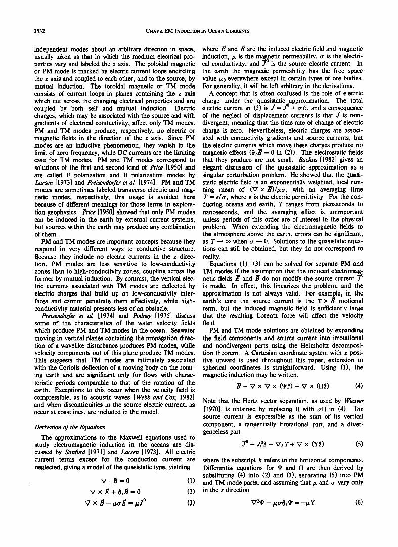
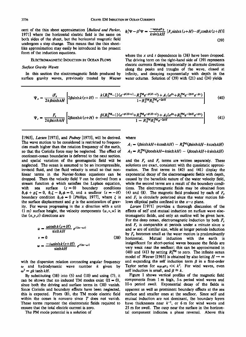
Figure 1 shows vertical profiles of the magnetic field components from 1 m high, 5-s period wind waves and 10-s period swell. Exponential decay of the fields is apparent as well as prominent boundary effects at the sea surface and smaller ones at the seafloor. Since self and

mutual induction are not dominant, the boundary layers have thicknesses near k -1, or 6 m for wind waves and 25 m for swell. The cusp near the surface in the horizontal component indicates a phase reversal. Above this


point the magnetic field is circularly polarized and retro- grade, and the sense reverses below it.

Model power spectra for wind waves and swell-induced electromagnetic fields can be obtained by combining (40)-(41), which give the field amplitude per unit wave height, with the Pierson-Moskowitz amplitude variance spectrum [Phillips, 1977]

E((o) -- 2•rag2' e -0'74((ø/(øm)-4 (42) (o 5

with (om the peak frequency, where the phase velocity of the waves equals that of the wind producing it, and a is a semi-empirical, dimensionless constant in the range 0.001-0.006. The Pierson-Moskowitz spectrum represents the statistical effects of complex, nonlinear wave-wave interactions and wave breaking. The advantage of combining (42) with (40)-(41) is that the electromagnetic spectra are independent of wave height and depend only on the distribution of wave periods. Theoretical spectra are contained in the work by Chave and Cox [1982] and are qualitatively like those obtained by Fraser [1966].

Kelvin Wave

3OO

ß 200

,,, 100

-r 0

I-

0 3000 6000

• •oo

,,, 0

• -100

0 '30'00' '60'00 OFFSHORE DISTANCE (km)

9 •.s ,.-' 1.0

_(2 0.5

•- 0.0 0 3000 6000

'" OFFSHORE DISTANCE (km)

OFFSHORE DISTANCE (krn)

> 1.0

J o.s 9 0.6 ,-7 0.4

o_ 0.2

• o.o '• ' '30'00' '60'00


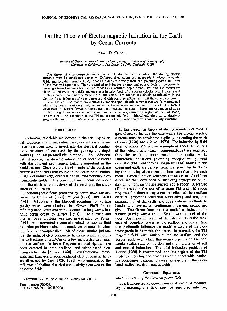
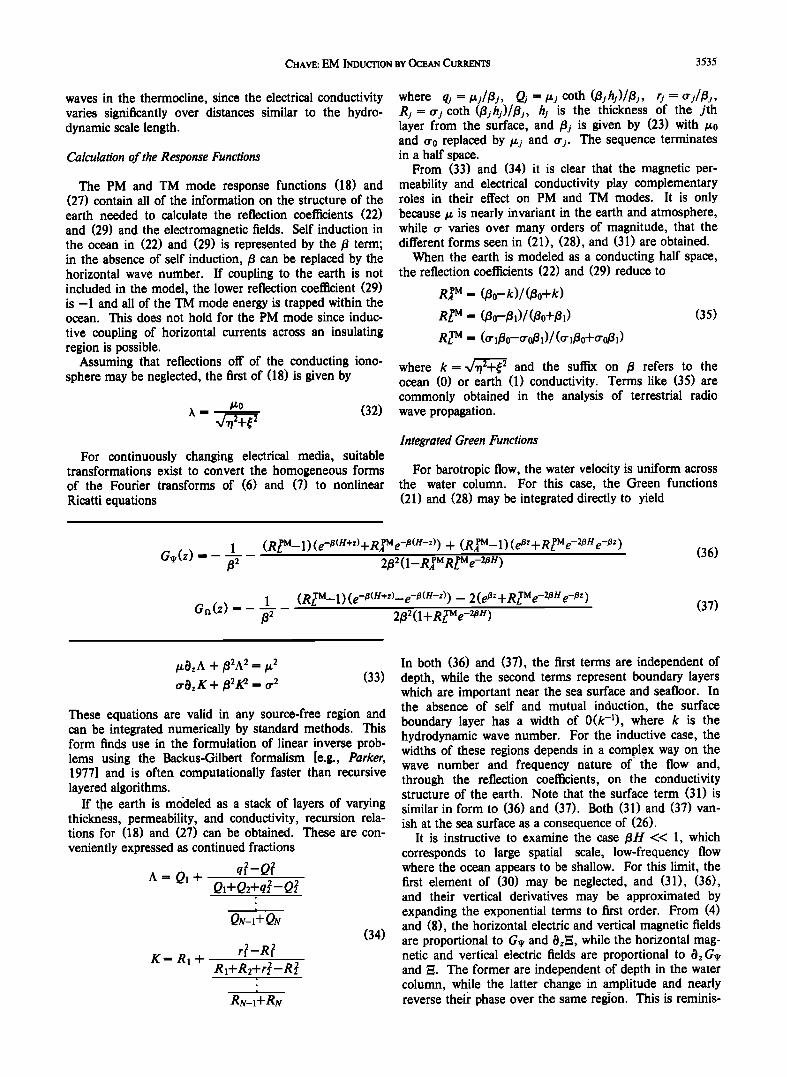
Fig. 2. The horizontal electric (left panels) and vertical electric (right panels) field amplitude and phase observed at the seafloor from a Kelvin wave propagating north along the California coast at 30øN with a surface height of 1 m at the coastline. The ocean depth is taken as 4 km, the seawater conductivity is 3.2 S m -1, and the mantle consists of a 100 km insulator overlying a 0.05 Sm -1 half space. The horizontal fields are separated into offshore (solid) and longshore (dashed) components.

Kelvin waves are often used as tide models due to their

analytic simplicity and their consistency with coastal observations of sea level [Hendershott, 1981]. Due to the low frequency of the tides, the Coriolis force plays a prominent part in the dynamics, and both PM and TM mode contributions to the electromagnetic fields are expected.

Tidal flow is governed by the Laplace tidal equations

with astronomical driving forces whose form is well determined. Kelvin waves are coastally trapped, nondispersive, free progressive wave solutions of the linearized shallow water equations

Ot u -- fv = --gOx•

Ot v Jr' fu =--gC•y• 8t• + H(OxU+OyV)= 0

(43)

120

z 40

• o

MAONETIC FIELD (nT)

10-7 10-5 10-3 10-1

i i i

/ /

MAGNETIC FIELD (nT)

120

z 40

• o

10-7 10-5 10-3 10-1 i ' i !

• ,,'

Fig. 1. Vertical profiles of the induced horizontal (top) and vertical (bottom) magnetic fields produced by one meter high surface gravity waves of 5-s (solid lines) and 10-s (dashed lines) period in a 100-m-deep ocean. The geomagnetic field has an amplitude of 3 x 104 nT, and the ocean conductivity is 3.2 S m -] while the earth conductivity is 0.05 S m -1. Horizontal lines are drawn to indicate the seafloor at 0 m and the sea surface at 100 m. The cusp in the top panel seen near the sea surface indicates a 180 ø change in the phase of the horizontal magnetic field.

where •; is the sea surface displacement, H is the constant ocean depth, and f--211sink is the Coriolis parameter, with 11 the rotation frequency of the earth and X the latitude. For fixed X, (43) are physical descriptions on a flat f plane which is tangent to the earth at the given latitude. The solution for a coastline along x--0, with the ocean occupying x •< 0,-H •< z •< 0, is given by

• ---- ek(f/o,)x ei(ky-(ot) u=O

(44) v= gk

z

w = -i(o(• + 1)(; for a unit (1 m) surface displacement, and the hydrodynamic dispersion relation is (o 2 -- gHk 2 connecting angular frequency (o and hydrodynamic wave number k for shallow water waves. The coordinates (x,y) refer to the offshore and longshore directions. The surface displacement and longshore velocity both decay exponentially offshore at a rate that is dependent on both water depth and latitude, while there is no offshore velocity component. The vertical velocity component may be neglected since w/v = O(kH) << 1. The longshore wavelength is quite large: for a water depth of 4 km at the semidiurnal period, k -1 -- 1350 kin. It is convenient to re-express (44) in geographic coordinates, denoted by primes, for a coastline striking at a clockwise angle a with respect to geographic north (u'= v sin a, v'= v cos a). The


cn 100

0

< -100

i i

0 3000 60•00 OFFSHORE DISTANCE (km)

• 100

,., 0

• -lOO

0 ' 30•00 ' "60•00 OFFSHORE DISTANCE (km)

=12

• 8

z • 0 < 0 3000 6000

OFFSHORE DISTANCE (km)

I

0 •30•00 6000 OFFSHORE DISTANCE (kin)

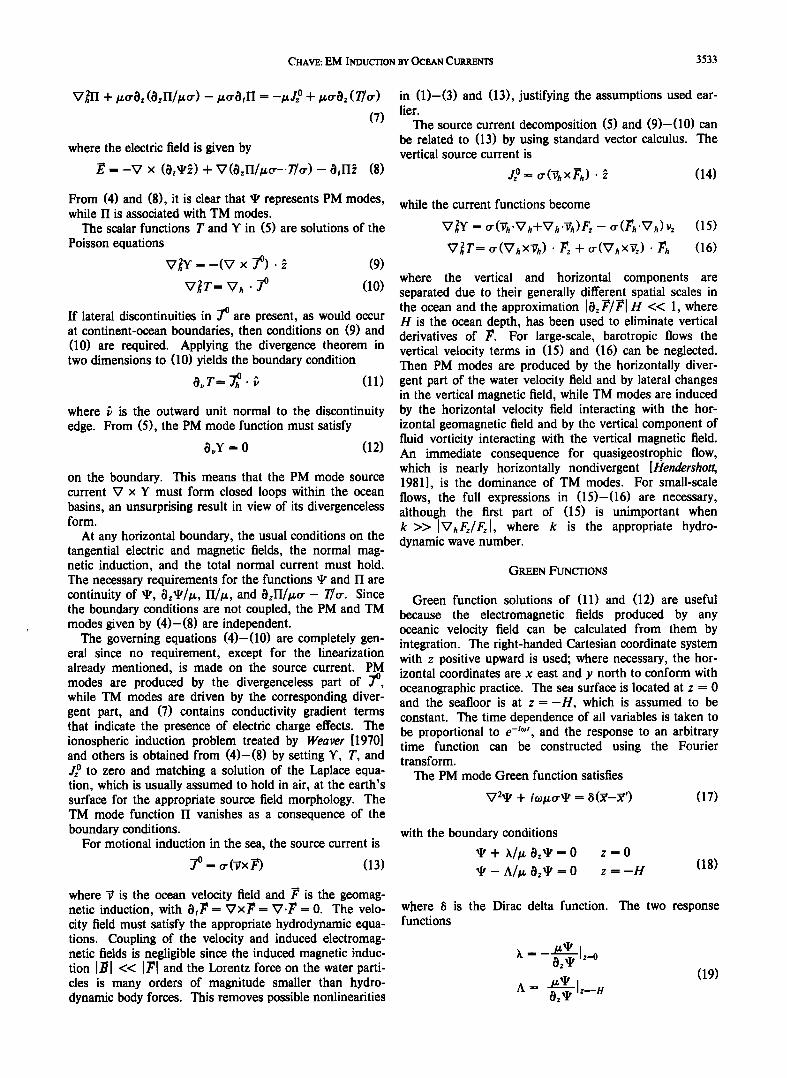
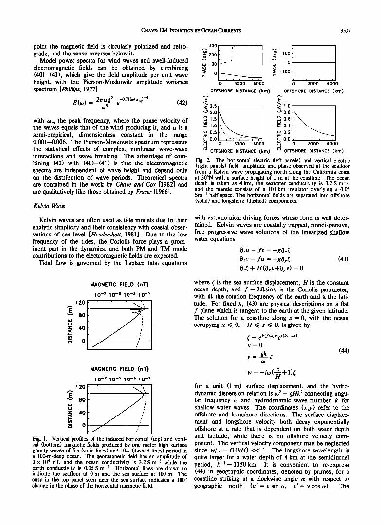
Fig. 3.' The magnetic field components for the model of Figure 2. See Figure 2 caption for details.

geomagnetic field is assumed to be geocentric with the two components Fy' = F0cosh, Fz' = -2F0sinh, where F0 • 3.7 x 10 4 nT is the geomagnetic field strength.

Since points near the coastline (i.e., within one hydrodynamic wavelength) are of special interest, the boundary conditions on (9) and (10) given by (11) and (12) must be used in separating the source current terms, to yield

i oJo-ogFz • ¾---- f2_oo2 [ek(f/a')x--eløc] (45)

o9 o-ogFz •

f2-co2 • ek(f/,,,)X_ekX (46)

jz o = trogkFy'sinot ekCr/,,,)x (47)

where the y and t dependence of (44) is understood. The vertical source current vanishes for north-south striking coastlines. In the absence of rotation (f--0), the TM mode source currents do not vanish, and (46) in particular exists as a consequence of the coastline discontinuity in 70 and (11)-(12). This means that the electromagnetic fields induced by shallow water waves (e.g., tsunamis) propagating along the coastline exhibit exponential offshore decay, a fact noted previously by Larsen [1968].

Taking Fourier transforms in the x coordinate of (45)-(47), substituting into (21)-(24) and (28)-(31), and using (36)-(37) gives the PM and TM mode potential functions

-i(otxoo'ogFz' [ 1 1 • = f2-o02 k(f/•)-t-i• G.(z) (48)

[ kF•'sin(z Gn (z) fI = --/xoo'og •(k(f /•)-Fi'rl)

f2--O•2 flea 1 '] • (z) k(f /•)+iw k+i•q (49)

where (k+i•o) -1 is the one-sided (x •< 0) Fourier

transform of e •. The offshore variation is recovered

using (20), while the longshore and time dependences are identical to that of (44). The electromagnetic fields are easily obtained by applying (4) and (8).

The assumption that the conductivity of the continent occupying x > 0, -H •< z •< 0 is identical to that of the ocean is implicit in (48) and (49). While this is not a realistic model of the earth since continental material has a

low electrical conductivity, the electromagnetic fields are insensitive to the nature of the coast-continent transition

at offshore distances much larger than a few times the depth of the ocean. Mathematical proof of this is presented in the appendix. Since significant differences between the electrical conductivity under the oceans and continents probably extends to depths of 10-100 km, the real zone over which (48)-(49) are in error is somewhat larger than a few kilometers, but it is not nearly as large as an inverse hydrodynamic wavelength k -1.

Figures 2 and 3 show the electric and magnetic fields as a function of offshore distance from a Kelvin wave of 1-m

surface displacement at the shore of a 4-km-deep ocean propagating north along the California coast at 30øN. The earth conductivity model consists of a nearly insulating (5 x 10 -7 S m-l), 100-km-thick layer overlying a 0.05 S m -1 half space. The deep conductivity is like that observed in magnetotelluric experiments [Filloux, 1981]. The hydrodynamic parameters and conductivity model are similar to those used by Larsen [1968], although his computational method was totally different. Larsen invoked the thin sheet approximation for the ocean, modeled the earth as an insulator overlying a superconducting mantle at 150km depth, made the continent an insulator, and solved the Maxwell equations numerically. The solutions of Figures 2 and 3 are nearly identical to those of Figure 6 of Larsen [1968] except for a 180 ø phase difference caused by different choice of horizontal coordinate orientation. The induced TM mode is zero, but a large electrostatic term given by (46) in (8) dominates the electric field and swamps the induced PM mode component. The vertical

300

• 200

w 100

'r 0

0 3000 6000


2.5

'•2.0

1.,5

1.o

0.5

0.0

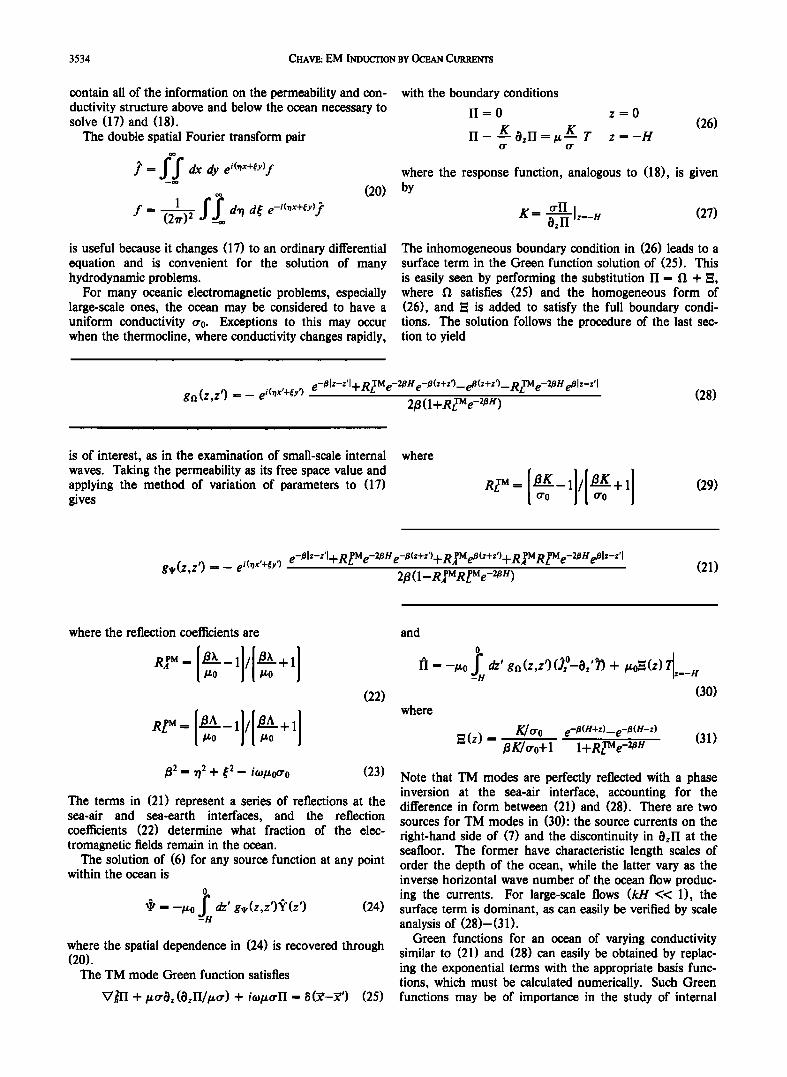
Fig. 4.

100

0

-100 !

6' 'o'oo' 6ooo OFFSHORE DISTANCE (kin)

> 1.0

ß 3 0.8 5 0.6 D. 0.4

ß __. 0.2

., ,"-,- • - ,-"'"•%•,, •o.o 0 3000 6000 ,., •) ' ,30•00 • '60'00

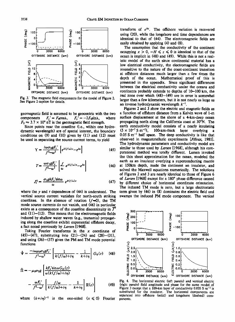
OFFSHORE DISTANCE (km) "' OFFSHORE DISTANCE (km) The horizontal electric (left panels) and vertical electric

(right panels) field amplitude and phase for the same model of Figure 3 except that a 100-km layer of conductivity 0.005 S m -1 is substituted for the insulator. The horizontal components are separated into offshore (solid) and longshore (dashed) components.


electric field is the open circuit value -Jzø/O'o, since no current flows through the insulating seafloor. Larsen's results with an insulating continent show transient differences in a zone a few tens of kilometers wide cen-

tered on the coast, especially in the vertical magnetic field, validating the conclusions of the appendix.

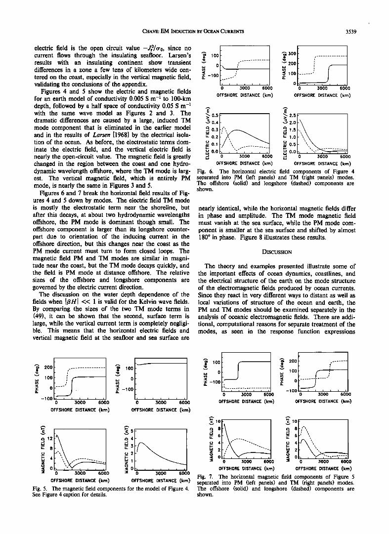
Figures 4 and 5 show the electric and magnetic fields for an earth model of conductivity 0.005 S m -• to 100-km depth, followed by a half space of conductivity 0.05 S m -• with the same wave model as Figures 2 and 3. The dramatic differences are caused by a large, induced TM mode component that is eliminated in the earlier model and in the results of Larsen [1968] by the electrical isola- tion of the ocean. As before, the electrostatic terms dom- inate the electric field, and the vertical electric field is nearly the open-circuit value. The magnetic field is greatly changed in the region between the coast and one hydrodynamic wavelength offshore, where the TM mode is largest. The vertical magnetic field, which is entirely PM mode, is nearly the same in Figures 3 and 5.

Figures 6 and 7 break the horizontal field results of Fig- ures 4 and 5 down by modes. The electric field TM mode is mostly the electrostatic term near the shoreline, but after this decays, at about two hydrodynamic wavelengths offshore, the PM mode is dominant though small. The offshore component is larger than its longshore counterpart due to orientation of the inducing current in the offshore direction, but this changes near the coast as the PM mode current must turn to form closed loops. The magnetic field PM and TM modes are similar in magnitude near the coast, but the TM mode decays quickly, and the field is PM mode at distance offshore. The relative

sizes of the offshore and longshore components are governed by the electric current direction.

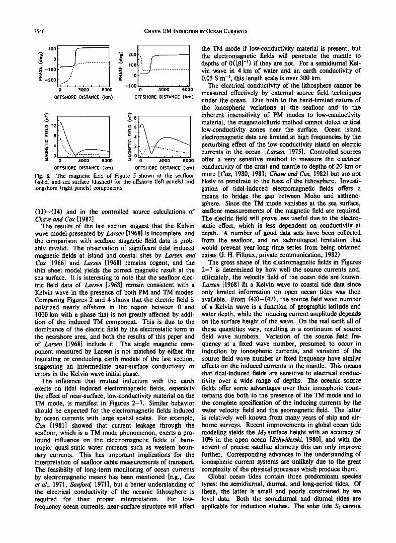
The discussion on the water depth dependence of the fields when ]13HI << 1 is valid for the Kelvin wave fields. By comparing the sizes of the two TM mode terms in (49), it can be shown that the second, surface term is large, while the vertical current term is completely negligible. This means that the horizontal electric fields and

vertical magnetic field at the seafloor and sea surface are

100

0

-1 O0

0 3000 6000


30O

200

lOO .......

, 'o'oo' 'o'oo OFFSHORE DISTANCE (km)

•o.4 9 0.3 "0.2

•,o.1 o o.o

• 1.s

• 1.0

• 0.5

0 3000 6000 • 0.0 OFFSHORE DISTANCE (km)

0 3000 6000


Fig. 6. The horizontal electric field components of Figure 4 separated into PM (left panels) and TM (right panels) modes. The offshore (solid) and longshore (dashed) components are shown.

nearly identical, while the horizontal magnetic fields differ in phase and amplitude. The TM mode magnetic field must vanish at the sea surface, while the PM mode component is smaller at the sea surface and shifted by almost 180 ø in phase. Figure 8 illustrates these results.

DISCUSSION

The theory and examples presented illustrate some of the important effects of ocean dynamics, coastlines, and the electrical structure of the earth on the mode structure

of the electromagnetic fields produced by ocean currents. Since they react in very different ways to distant as well as local variations of structure of the ocean and earth, the PM and TM modes should be examined separately in the analysis of oceanic electromagnetic fields. There are additional, computational reasons for separate treatment of the modes, as seen in the response function expressions

a• 200 ..........

-r 0

-lOO o 3000' ' 60'00


.•

,., 0

• -lOO

o o'oo o'oo OFFSHORE DISTANCE (km)

" 8

_o • 4 z

< 0 :• o 3000 6ooo


•0 .... 0 3000 6000


Fig. 5. The magnetic field components for the model of Figure 4. See Figure 4 caption for details.

100

0

-100

0 30'00' 6000 OFFSHORE DISTANCE (km)

200

100

o

-lOO 0 3000 6000


clo

o 8

-• 6

o 4

'-' 2 z

< 0

• lO

• 4

<• o 0 3000 6000 •


0 3000 6000


Fig. 7. The horizontal magnetic field components of Figure 5 separated into PM (left panels) and TM (right panels) modes. The offshore (solid) and longshore (dashed) components are shown.


lOO

o

-100

-200

'o'oo' 'o'oo OFFSHORE DISTANCE (km)

2OO

100

-100 0 ,50'00 60'00 OFFSHORE DISTANCE (kin)

•12

" 8

•'- 4 z

< 0-, ?'-,-; - - i

'• 0 ,5000 6000


0 3000 6000

OFFSHORE DISTANCE (kin)

Fig. 8. The magnetic field of Figure 5 shown at the seafloor (solid) and sea surface (dashed) for the offshore (left panels) and longshore (right panels) components.

(33)-(34) and in the controlled source calculations of Chave and Cox [1982].

The results of the last section suggest that the Kelvin wave model presented by Larsen [1968] is incomplete, and the comparison with seafloor magnetic field data is probably invalid. The observation of significant tidal induced magnetic fields at island and coastal sites by Larsen and Cox [1966] and Larsen [1968] remains cogent, and the thin sheet model yields the correct magnetic result at the sea surface. It is interesting to note that the seafloor electric field data of Larsen [1968] remain consistent with a Kelvin wave in the presence of both PM and TM modes. Comparing Figures 2 and 4 shows that the electric field is polarized nearly offshore in the region between 0 and 1000 km with a phase that is not greatly affected by addition of the induced TM component. This is due to the dominance of the electric field by the electrostatic term in the nearshore area, and both the results of this paper and of Larsen [1968] include it. The single magnetic component measured by Larsen is not matched by either the insulating or conducting earth models of the last section, suggesting an intermediate near-surface conductivity or errors in the Kelvin wave initial phase.

The influence that mutual induction with the earth

exerts on tidal induced electromagnetic fields, especially the effect of near-surface, low-conductivity material on the TM mode, is manifest in Figures 2-7. Similar behavior should be expected for the electromagnetic fields induced by ocean currents with large spatial scales. For example, Cox [1981] showed that current leakage through the seafloor, which is a TM mode phenomenon, exerts a pro- found influence on the electromagnetic fields of barotropic, quasi-static water currents such as western boundary currents. This has important implications for the• interpretation of seafloor cable measurements of transport. The feasibility of long-term monitoring of ocean currents by electromagnetic means has been mentioned [e.g., Cox et al., 1971; Sanford, 1971 ], but a better understanding of the electrical conductivity of the oceanic lithosphere is required for their proper interpretation. For low- frequency ocean currents, near-surface structure will affect

the TM mode if low-conductivity material is present, but the electromagnetic fields will penetrate the mantle to depths of 0<ll if they are not. For a semidiurnal Kel- vin wave in 4 km of water and an earth conductivity of 0.05 S m -1, this length scale is over 300 km.

The electrical conductivity of the lithosphere cannot be measured effectively by external source field techniques under the ocean. Due both to the band-limited nature of

the ionospheric variations at the seafloor and to the inherent insensitivity of PM modes to low-conductivity material, the magnetotelluric method cannot detect critical low-conductivity zones near the surface. Ocean island electromagnetic data are limited at high frequencies by the perturbing effect of the low-conductivity island on electric currents in the ocean [Larsen, 1975]. Controlled sources offer a very sensitive method to measure the electrical conductivity of the crust and mantle to depths of 20 km or more [Cox, 1980, 1981; Chave and Cox, 1982] but are not likely to penetrate to the base of the lithosphere. Investi- gation of tidal-induced electromagnetic fields offers a means to bridge the gap between Moho and astheno- sphere. Since the TM mode ,vanishes at the sea surface, seafloor measurements of the magnetic field are required. The electric field will prove less useful due to the electrostatic effect, which is less dependent on conductivity at depth. A number of good data sets have been collected from the seafloor, and no technological limitation that would prevent year-long time series from being obtained exists (J. H. Filloux, private communication, 1982).

The gross shape of the electromagnetic fields in Figures 2-7 is determined by how well the source currents and, ultimately, the velocity field of the ocean tide are known. Larsen [1968] fit a Kelvin wave to coastal tide data since only limited information on open ocean tides was then available. From (43)-(47), the source field wave number of a Kelvin wave is a function of geographic latitude and water depth, while the inducing current amplitude depends on the surface height of the wave. On the real earth all of these quantities vary, resulting in a continuum of source field wave numbers. Variation of the source field fre-

quency at a fixed wave number, presumed to occur in induction by ionospheric currents, and variation of the source field wave number at fixed frequency have similar effects on the induced currents in the mantle. This means that tidal-induced fields are sensitive to electrical conduc-

tivity over a wide range of depths. The oceanic source fields offer some advantages over their ionospheric coun- terparts due both to the presence of the TM mode and to the complete specification of the inducing currents by the water velocity field and the geomagnetic field. The latter is relatively well known from many years of ship and air- borne surveys. Recent improvements in global ocean tide modeling yields the M2 surface height with an accuracy of 10% in the open ocean [Schwiderski, 1980], and with the advent of precise satellite altimetry this can only improve further. Corresponding advances in the understanding of ionospheric current systems are unlikely due to the great complexity of the physical processes which produce them.

Global ocean tides contain three predominant species types' the semidiurnal, diurnal, and long-period tides. Of these, the latter is small and poorly constrained by sea level data. Both the semidiurnal and diurnal tides are applicable for induction studies. The solar tide S2 cannot


be used due to the very large solar heating effect on its ionospheric part. The magnetic field at the semidiurnal M2 tidal frequency contains at most a limited ionospheric part [Larsen, 1968], and its diurnal counterpart should behave in a similar way. The influence of ionospheric parts on the fields can be removed by comparing seafloor data to observatory data at inland sites for similar geomagnetic latitudes.

One potentially important quantity has been neglected in the analysis of this paper: the influence of seafloor topography in the electromagnetic fields. Sanford [1971] and Sklarz [1975] have applied perturbation methods to electromagnetic induction by large-scale ocean flow to examine this effect. They show that the largest change produced by topography is variation nf t_h_o. inducing currents by perturbation of the velocity field. This is accounted for by the tide model of Schwiderski [1980]. Deflection of horizontal induced currents by the topography must also be considered, especially if the relief is large and the surface electrical conductivity is low [Sklarz, 1975]. Since the magnetic field is an integral measure of electrical current, the influence on it is expected to be smaller than for the electric field. Topographic corrections can be obtained by perturbation or boundary integral equation methods. In addition, only topography with a length scale that is a significant fraction of a tidal wavelength is expected to produce long distance changes in the electric currents, and small-scale topography can be neglected, except locally.

APPENDIX: EM INDUCTION BY A KELVIN WAVE FOR AN INSULATING CONTINENT

In the text, equations (6)-(7) for the driving currents given by (45)-(47) are solved for the ocean in x--0, -H •< z •< 0, when the continent in x > 0, -H •< z •< 0 has the same conductivity as the ocean. Additional conditions on (6)-(7) are required if the continent is modeled as an insulator, a far more realistic approximation. In both cases the mantle conductivity is the same under both oceans and continents, neglecting possible deep structural differences between them.

Consider first the insulating seafloor and continent model used by Larsen [1968]. In the text it is shown that the insulating seafloor requires II--0 in the ocean. For an insulating continent the total electric current Jx must vanish at the continent edge, requiring that • = 0 at x = 0. Using the linearity of (6), the solution is separated into • = •0+ •1, where •0 is given by (48) and •1 satisfies

8z2Xt rl -- •2xtrl = 0 xtrl--0 on z--O, z=-H (A1)

The solution is expressible as a Fourier series

= ,,o .•, j27r 2 XlI1 E ,4• sin j•z exp •2+ x (A2) j--1 H' /./2

where the coefficients •lj are found by applying the condition •=0 at x--0 in the usual way. Due to the exponential term in (A2), the new term •1 decays/very quickly with x and is vanishingly small for x greater than

a few times -H. This accounts for the similarity of Fig- ures 5 and 6 to the results of Larsen [1968].

For a conductive seafloor, the solutions proceed in a similar way. At the continent edge, the tangential electric and magnetic fields and the normal magnetic induction must be continuous and the normal electric current must vanish, requiring that

ikOz•O - OxII0-- ikOz•c

O•Oz*0 + ikIIo = O•Oz*c (A3)

-o#xoo'ok•o + 8xOzHo-- 0

at x -- 0. The subscripts refer to the ocean and continent. *c satisfies Laplace's equation with boundary conditions given at x = 0 by (A3), at z -- -H given by (18) for zero conductivity, and finiteness conditions as x and z approach infinity. The solution in the continent is of no interest, and (A3) can be rearranged to give

OxOzIIo •o -- (^4)

o#•oo'ok

on x = 0. The potential is expanded as before into the zero-order solutions (48) and (49) and the first-order boundary terms. Fourier series like (A2) still appear, and the new terms are significant only near the boundary. The effect is one of mode conversion from TM into PM modes in a narrow boundary layer. Additional correction for current leakage through the mantle into the continent must be made; this is a two-dimensional problem not treated here.

,4cknowledgments. C.S. Cox provided his usual, unique physical insight during many fruitful discussions throughout this work. His interest in electromagnetic induction by ocean tides, stretching back nearly 20 years, provided the impetus for this investigation. R.L. Parker and G. Backus clarified some troublesome mathematical details. This work was supported by the National Science Foundation under grants OCE81-10399 and EAR 81-20949 and by the Office of Naval Research.

REFERENCES

Backus, G., The electric field produced in the mantle by the dynamo in the core, Phys. Earth Planet. Inter., 28, 191-214, 1982.

Bullard, E. C., and R. L. Parker, Electromagnetic induction in the oceans, in The Sea, V.4 Pt. 2, edited by A. E. Maxwell, pp. 695-730, Wiley, New York, 1971.

Chave, A.D., and C. S. Cox, Controlled electromagnetic sources for measuring electrical conductivity beneath the oceans, 1, Forward problem and model study, J. Geophys. Res., 87, 5327-5338, 1982.

Cox, C. S., Electromagnetic induction in the oceans and infer- ences on the constitution of the earth, Geophys. Surv., 4, 137-156, 1980.

Cox, C. S., On the electrical conductivity of the oceanic lithosphere, Phys. Earth Planet. Inter., 25, 196-201, 1981.

Cox, C. S., J. H. Filloux, and J. C. Larsen, Electromagnetic studies of ocean currents and the electrical conductivity below the seafloor, in The Sea, V.4 Pt.2, edited by A. E. Maxwell, pp. 637-693, Wiley, New York, 1971.

Filloux, J. H., Magnetotelluric exploration of the North Pacific: Progress report and preliminary soundings near a spreading ridge, Phys. Earth Planet. Inter., 25, 187-195, 1981.

Fraser, D.C., The magnetic fields of ocean waves, Geophys. J. R. astron. Soc., 11, 507-517, 1966.

Hendershott, M., Long waves and ocean tides, in Evolution of Phy- sical Oceanography, edited by B. A. Warren and C. Wunsch, pp. 292-341, MIT Press, Cambridge, Mass., 1981.


Larsen, J. C., Electric and magnetic fields induced by deep sea tides, Geophys. J. R. •4stron. Soc., 16, 47-70, 1968.

Larsen, J. C., The electromagnetic field of long and intermediate waves, J. Mar. Res., 29, 28-45, 1971.

Larsen, J. C., An introduction to electromagnetic induction in the ocean, Phys. Earth Planet. Inter., 7, 389-398, 1973.

Larsen, J. C., Low frequency (0.1-6.0 cpd) electromagnetic study of deep mantle electrical conductivity beneath the Hawaiian Islands, Geophys. J. R. •lstron. Soc., 43, 17-46, 1975.

Larsen, J. C., and C. S. Cox, Lunar and solar daily variation in the magnetotelluric field beneath the ocean, J. Geophys. Res., 71, 4441-4445, 1966.

Parker, R. L., Understanding inverse theory, /lnnu. Rev. Earth Planet. Sci., 5, 35-64, 1977.

Phillips, O. M., The Dynamics of the Upper Ocean, 2nd ed., Cam- bridge University Press, Cambridge, 336 pp, 1977.

Podney, W., Electromagnetic fields generated by ocean waves, J. Geophys. Res., 80, 2977-2990, 1975.

Preisendorfer, R., J. C. Larsen, and M. A. Sklarz, Electromag- netic fields induced by plane-parallel, internal and surface ocean waves, Hawaii Inst. of Geophys. Tech. Rep. 74-7, Honolulu, 1974.

Price, A. T., Electromagnetic induction in a semi-infinite conduc- tor with a plane boundary, Q. J. Mech./lppl. Math., 3, 385-410, 1950.

Sanford, T. B., Motionally induced electric and magnetic fields in the sea, J. Geophys. Res., 76, 3476-3492, 1971.

Schwiderski, E., On charting global ocean tides, Rev. Geophys. Space Phys., 18, 243-268, 1980.

Sklarz, M. A., The effect of topography on the electromagnetic fields induced by plane-parallel barotropic ocean waves, Ph.D. dissertation, 306 pp, Univ. of Hawaii, Honolulu, 1975.

Weaver, J. T., Magnetic variations associated with ocean waves and swell, J. Geophys. Res., 70, 1921-1929, 1965.

Weaver, J. T., The general theory of electromagnetic induction in a conducting half space, Geophys. J. R./lstron. Soc., 22, 83-100, 1970.

Webb, S., and C. S. Cox, Electromagnetic fields induced at the seafloor by Rayleigh-Stonely waves, J. Geophys. Res., 87, 4093-4102, 1982.

(Received September 16, 1982; accepted December 30, 1982.)

on the theory of electromagnetic induction in the earth · pdf fileon the theory of...

Documents