NASA/TP—2013–217494

On the Trend of the Annual Mean, Maximum,and Minimum Temperature and the DiurnalTemperature Range in the Armagh Observatory,Northern Ireland, Dataset, 1844 –2012Robert M. WilsonMarshall Space Flight Center, Huntsville, Alabama

November 2013

�������������� ������������

Since its founding, NASA has been dedicated to the advancement of aeronautics and space science. The �������������� ���������������������������������������������������������������������maintain this important role.

������������������������������������ ����!������"��������#���$������� ��������������%����������� �����������������&�������������������������������'� ������������the NASA STI Database, the largest collection of aeronautical and space science STI in the world. ������������������������������%�����(�����mechanism for disseminating the results of its research and development activities. These results �����(������ �����������������������"�����������$�)��������( �����������)�������������*

+� �-#6��#�!��:;!�#�����&�"���������������� �����������������<�����������phase of research that present the results of NASA programs and include extensive data ��������������������&����( ���������������������������������� ��������� ���and information deemed to be of continuing reference value. NASA’s counterpart of peer-reviewed formal professional papers but has less stringent limitations on manuscript length and extent of graphic presentations.

+� �-#6��#�!�>->�"��?:>&���������� ���������� ������������������������������������@� ������$��&�&$�B(������������������$�)������������$�� ������������������������minimal annotation. Does not contain extensive �������&

+� #���"�#��"�"-��"�&���������� ���������� �����������C������� �contractors and grantees.

+� #��E-"-�#-��:;!�#�����&�#������ ���������������������� ������������������$���������$��������$����������������������� ������������� ��������&

+� ��-#��!��:;!�#�����&��������$��������$�or historical information from NASA programs, projects, and mission, often concerned with subjects having substantial public interest.

+� �-#6��#�!��"���!�����&� English-language translations of foreign

��������� �������������������������NASA’s mission.

Specialized services that complement the STI �������������%�� �'�����������������( ���������custom thesauri, building customized databases, organizing and publishing research results…even providing videos.

E��������������������(��������������������������$�������������)��*

• Access the NASA STI program home page at G��*JJ)))&��&���&��'K

+� -C�������(��B(�����'������������� G����L��&���&��'K

+� �����������������6����?������ 757 –864–9658

+� O�����*� ������������������?���� >��������QRU� �����!������"��������#���� 6����$�V��WXYUQZWQ[[$�:��

i

NASA/TP—2013–217494

On the Trend of the Annual Mean, Maximum, and Minimum Temperature and the Diurnal Temperature Range in the Armagh Observatory,Northern Ireland, Dataset, 1844–2012Robert M. WilsonMarshall Space Flight Center, Huntsville, Alabama

November 2013

National Aeronautics andSpace Administration

Marshall Space Flight Center • Huntsville, Alabama 35812

ii

Available from:

NASA STI Information DeskMail Stop 148

NASA Langley Research CenterHampton, VA 23681–2199, USA

757–864–9658

This report is also available in electronic form at<http://www.sti.nasa.gov>

TRADEMARKS

Trade names and trademarks are used in this report for identification only. This usage does not constitute an official endorsement, either expressed or implied, by the National Aeronautics and Space Administration.

iii

TABLE OF CONTENTS

1. INTRODUCTION ............................................................................................................. 1

2. RESULTS AND DISCUSSION ......................................................................................... 3

2.1 Annual and 10-yma Values of Armagh Surface Air Temperatures and Diurnal Temperature Range ................................................................................... 3

2.2 Decadal and Sunspot Cycle Averages of Armagh Surface Air Temperatures and Diurnal Temperature Range .................................................................................. 6

2.3 Scatter Plots of Armagh Surface Air Temperatures Against Selected Climate-Forcing Factors Using Decadal and Sunspot Cycle Averages ....................................... 16

2.4 Multivariate Fits ........................................................................................................... 28

3. SUMMARY ....................................................................................................................... 39

REFERENCES ....................................................................................................................... 41

iv

LIST OF FIGURES

1. Annual and 10-yma values of ASAT mean temperature for 1844–2012 ..................... 3

2. Annual and 10-yma values of (a) ASAT max and ASAT min temperature and (b) DTR for 1844–2012 ...................................................................................... 5

3. Annual values of NSD for 1849–2012 ....................................................................... 7

4. Annual and 10-yma values of (a) SSN for 1843–2012, (b) aa for 1868–2012, and (c) SSA for 1875–2012 ........................................................................................ 9

5. Decadal (interval) averages of (a) SSN, (b) aa, and (c) SSA. SC averages of (d) SSN, (e) aa, and (f) SSA .................................................................................. 12

6. ASAT mean: (a) Decadal (interval) average and (b) SC average ................................. 13

7. Decadal (interval) average of (a) ASAT max, (b) ASAT min, and (c) DTR; SC average of (d) ASAT max, (e) ASAT min, and (f) DTR ....................................... 14

8. Decadal (interval) averages of (a) ASAT mean versus aa, (b) ASAT max versus aa, and (c) ASAT min versus aa; SC averages of (d) ASAT mean versus aa, (e) ASAT max versus aa, and (f) ASAT min versus aa .............................. 17

9. Annual and 10-yma values of (a) NAO for 1843–2012 and (b) AMO for 1856–2012 ............................................................................................................ 19

10. Annual and 10-yma values of (a) SOI for 1876–2012 and (b) PDO for 1900–2012 ............................................................................................................ 20

11. Decadal (interval) averages of (a) NAO, (b) AMO, (c) SOI, and (d) PDO; SC averages of (e) NAO, (f) AMO, (g) SOI, and (h) PDO ......................................... 23

12. MLCO2: (a) Annual values for 1959–2012, (b) decadal (interval) averages, and (c) SC averages ................................................................................................... 24

13. MLCO2: (a) Decadal averages of ASAT min versus decadal averages and (b) SC averages of ASAT min versus SC averages .............................................. 25

v

LIST OF FIGURES (Continued)

14. Decadal averages of (a) ASAT mean versus ASAT mean (aa, MLCO2), (b) ASAT max versus ASAT max (aa, MLCO2), and (c) ASAT min versus ASAT min (SOI, MLCO2); SC averages of (d) ASAT mean versus ASAT mean (aa, MLCO2), (e) ASAT max versus ASAT max (SOI, MLCO2), and (f) ASAT min versus ASAT min (PDO, MLCO2) .............................................. 30

15. First difference (fd) values based on decadal (interval) averages of (a) ASAT mean, (b) ASAT max, and (c) ASAT min; fd values based on SC averages of (d) ASAT mean, (e) ASAT max, and (f) ASAT min .............................................. 32

16. First difference (fd) values based on decadal (interval) averages of (a) aa, (b) NAO, (c) AMO, (d) SOI, (e) PDO, and (f) MLCO2; fd values based on SC averages of (g) aa, (h) NAO, (i) AMO, (j) SOI, (k) PDO, and (l) MLCO2 ...... 33

vi

LIST OF TABLES

1. Epochs and amplitudes for near sunspot cycle minimum .......................................... 11

2. Inferred regressions of y versus x using decadal averages and SC averages ................ 26

3. Results of multivariate fitting .................................................................................... 28

4. First differences of parametric decadal and SC averages ........................................... 31

5. Estimates of ASAT mean, max, and min for interval 17 (2010–2019) and SC24 using the inferred multivariate fits in conjunction with last known parametric values and the means of the parametric fd values, except for MLCO2 ...................... 35

6. Comparison of decadal and SC parametric values for intervals 16 (2000–2009) and 17 (2010–2019), and SC23 (1996–2007) and 24 (2008–present) ........................... 37

7. Monthly parametric values for 2013 .......................................................................... 38

vii

LIST OF ABBREVIATIONS AND ACRONYMS

10-yma 10-year moving average

aa aa (antipodal) geomagnetic index

aa min aa minimum amplitude

AMO Atlantic Multidecadal Oscillation (index)

ASAT Armagh surface air temperature

ASAT max ASAT maximum annual temperature

ASAT mean ASAT mean annual temperature, equal to (ASAT max + ASAT min)/2

ASAT min ASAT minimum annual temperature

DTR diurnal (daily) temperature range, equal to ASAT max – ASAT min

fd first difference

MLCO2 Mauna Loa carbon dioxide (index)

NAO North Atlantic Oscillation (index)

NOAA National Oceanic and Atmospheric Administration

NSD number of spotless days

NSD max NSD maximum amplitude

ONI Oceanic Niño Index

PDO Pacific Decadal Oscillation (index)

SC sunspot cycle

SOI Southern Oscillation Index

SSA sunspot area

SSA min SSA minimum amplitude

SSN sunspot number

SSN min SSN minimum amplitude

SST sea surface temperature

THC thermohaline circulation

USAF United States Air Force

viii

NOMENCLATURE

a y intercept

b slope

cl confidence level

n sample size (number)

Ry12 multivariate coefficient of correlation

R2y12 multivariate coefficient of determination

r coefficient of correlation

r2 coefficient of determination

Sy12 multivariate standard error of the estimate

sd standard deviation

se standard error of estimate

t t statistic for independent samples

x independent variable

x1 independent variable 1

x2 independent variable 2

y dependent variable

y′ alternate dependent variable

y″ alternate dependent variable

z normal deviate for the sample

1

TECHNICAL PUBLICATION

ON THE TREND OF THE ANNUAL MEAN, MAXIMUM, AND MINIMUM TEMPERATURE AND THE DIURNAL TEMPERATURE RANGE IN THE ARMAGH

OBSERVATORY, NORTHERN IRELAND, DATASET, 1844–2012

1. INTRODUCTION

One of the longest thermometer-based temperature records available for study is that of the Armagh Observatory, Northern Ireland.1–8 The Armagh meteorological station is located near the center of the Observatory grounds about 1 km northeast of the ancient city of Armagh, Northern Ireland, being situated about 64 m above sea level at the top of a small hill in an estate of natural woodland and parkland that measures about 7 ha (about 20 acres). Previous studies have shown that its rural environment has ensured that the temperature measurements suffer little to no urban microclimatic effects and that the Armagh temperature record serves as a good proxy for monitoring long-term trends in global and northern hemispheric surface air temperatures.4,5

Although the Armagh temperature record extends back to 1795, the most complete and reli-able (i.e., calibrated) temperature data extends back only to 1844, owing to the introduction and routine use of daily-read temperatures from maximum and minimum thermometers that began there in 1843. The Armagh surface air temperature (ASAT) dataset is accessible online at <http://climate.arm.ac.uk/scan.html>.

It has long been recognized that the Sun, being the source of energy input into the Earth’s climate system, acts as a major climate change forcing factor, especially for the preindustrial era.9–17 Evidence5,7,8 has also been described indicating some degree of solar cycle forcing and secular varia-tion in the ASAT data during the postindustrial era as well. However, because of the recent decrease in solar activity, concurrent with a continuing rise in surface air temperature, it is apparent that fac-tors other than solar forcing alone now dominate Earth’s climate system.8,18–21

One particular aspect of the continued warming has been a reduction over time in the differ-ence between the mean annual maximum and minimum temperatures, called the diurnal (or daily) temperature range (DTR). For example, Karl et al.22,23 have noted that a reduction in the DTR has been seen worldwide and that the reduction has occurred over an extended period of time, appar-ently related to a faster increase in higher minimum temperatures in comparison to the increase in maximum temperatures. Also, Easterling et al.24 have noted that inclusion of urban effects on the DTR appears negligible, whether measured using globally- or hemispherically-averaged time series. Likewise, Vose et al.25 have found that, on average, the minimum temperature increased more rapidly than the maximum temperature from 1950 to 2004, resulting in a significant DTR decrease that was

2

only evident during the interval 1950–1980. Many other studies from numerous countries around the world have found similar findings.26–41

In this study, the ASAT dataset is examined to determine the annual and 10-year moving aver-age (10-yma) variation of the mean (ASAT mean), maximum (ASAT max), and minimum (ASAT min) temperatures and its DTR for the interval 1844–2012. The temperature data are also examined in terms of decadal averages and sunspot cycle (SC) averages (i.e., the data are averaged over each SC, from sunspot cycle minimum to the next cycle minimum). Additionally, comparisons are made against the variations of sunspot number (SSN), the aa-geomagnetic index (aa), the sunspot area (SSA), the North Atlantic Oscillation (NAO) index, the Atlantic Multidecadal Oscillation (AMO) index, the Southern Oscillation Index (SOI), the Pacific Decadal Oscillation (PDO) index, and the Mauna Loa carbon dioxide (MLCO2) measurements in order to determine the relative strengths of the inferred statistical correlations between the ASAT data and these indices of climatic change.

3

2. RESULTS AND DISCUSSION

2.1 Annual and 10-yma Values of Armagh Surface Air Temperatures and Diurnal Temperature Range

Figure 1 displays the annual (thin jagged line) and 10-yma (thick smoothed line) values of the ASAT mean for the overall interval 1844–2012. The minimum annual ASAT mean measured 7.4 ºC in 1879 and the maximum (to date) annual ASAT mean measured 10.6 ºC in 2007, inferring an aver-age rate of increase in the annual ASAT mean of about 0.025 ºC yr–1 during the interval 1879–2007. In terms of the 10-yma values, used here to indicate trend, the minimum annual ASAT mean mea-sured 8.44 ºC in 1883 and the maximum annual ASAT mean measured 10.13 ºC in 2002 and 2003, inferring an average rate of increase in the 10-yma ASAT mean of about 0.014 ºC yr–1 during the interval 1883–2003. Overall, the average annual ASAT mean measures 9.25 ºC, having a standard deviation sd = 0.55 ºC. Use of the 10-yma values reduces the variance in the annual ASAT mean values by about 62%.

ASAT

Mea

n (°C

)

7

8

9

10

11 ASAT Mean (1844–2012)

1850 1900 1950 2000

7.4 °C (1879)

10.6 °C (2007)

Year

na = 85median = 9.21 °C

nb = 84nra = 32

��z = –3.3��nonrandom (cl>99.9%)

mean = 9.25 °Csd = 0.55 °C

Figure 1. Annual and 10-yma values of ASAT mean temperature for 1844–2012.

The median annual value of ASAT mean measures 9.21 ºC with 85 annual values equal to or larger than the median and 84 annual values smaller than the median, occurring in 32 positive- valued runs. Runs-testing42 yields the normal deviate for the sample z = –3.3, inferring that the annual ASAT mean values are distributed nonrandomly at confidence level cl >99.9%. Hence, the increase (trend) over time of ASAT mean is inferred to be real and statistically meaningful (important).

Examination of the 10-yma values of ASAT mean reveals that it was trending downwards between 1849 and 1883, decreasing from 9.46 to 8.44 ºC (about –0.03 ºC yr–1). Following this decline,

4

it rose sharply to 9.11 ºC between 1883 and 1901 (about 0.037 ºC yr–1). It then remained fairly level until about 1927 when it began to rise once again, increasing to 9.58 ºC in 1945 (about 0.031 ºC yr–1). From 1945 until about 1982, the ASAT mean decreased from 9.58 to 9.05 ºC (about 0.014 ºC yr–1). From 1982 to 2003, the ASAT mean increased to its peak value (as seen, thus far) of 10.13 ºC (about 0.051 ºC yr–1). Since 2003, the 10-yma ASAT mean has measured, respectively, 10.1, 10.02, 10, and 10.01 ºC for the years 2004–2007. Ten-year moving averages of the ASAT mean are found to have exceeded the annual long-term mean of 9.25 ºC between 1849 and 1856, 1933 and 1963, and every year since 1985, with the current peak exceeding the earlier peak in 1849 by more than 0.6 ºC. The 10.6 ºC measured for the ASAT mean in 2007 is 2.45 sd higher than the long-term mean of 9.25 ºC and the 7.4 ºC measured in 1879 is 3.36 sd lower than the long-term mean.

Now, the annual ASAT mean is a derived quantity, being the average of the ASAT max and ASAT min, which are provided by the daily-read maximum and minimum thermometers used at Armagh. Figure 2 displays the annual and 10-yma values of the ASAT max and ASAT min for the interval 1844–2012 and it also shows the variation of the DTR, which is simply the difference between ASAT max and ASAT min. Visually, a strong resemblance is evident between ASAT mean, max, and min.

5

Arm

agh

Surfa

ce A

ir Te

mpe

ratu

re (°

C)Da

ily Te

mpe

ratu

re R

ange

(DTR

)

ASAT Maximum (1844–2012)

ASAT Minimum (1844–2012)

DTR = ASAT Maximum – ASAT Minimum (1844–2012)

15

14

13

12

11

10

8

7

6

5

4

3

9

8

7

6

5

na = 85nb = 84

nra = 36 ��z = –2.07��nonrandom (cl>95%)

median = 12.8 °C

na = 85nb = 84

nra = 31 ��z = –3.61��nonrandom (cl>99.9%)

median = 5.65 °C

na = 85nb = 84

nra = 32 ��z = –3.3��nonrandom (cl>99.9%)

median = 7.19 °C

10.76 °C (1879)

4.04 °C (1879)

8.16 °C (1859)

6.96 °C (1997)

6.3 °C (1998)

14.42 °C (2007)

mean = 12.86 °Csd = 0.59 °C

mean = 5.64 °Csd = 0.56 °C

mean = 7.21 °Csd = 0.35 °C

20001950Year

19001850(b)

(a)

Figure 2. Annual and 10-yma values of (a) ASAT max and ASAT min temperature and (b) DTR for 1844–2012.

6

The ASAT max is found to vary nonrandomly (z = –2.07, cl >95%) between 10.76 ºC in 1879 and 14.42 ºC in 2007 and the mean ASAT max measures 12.86 ºC, having sd = 0.59 ºC. The ASAT min likewise is found to vary nonrandomly (z = –3.61, cl >99.9%) between 4.04 ºC in 1879 and 6.96 ºC in 1997 and the mean ASAT min measures 5.64 ºC, having sd = 0.56 ºC. Based on 10-yma values, ASAT max and ASAT min have ranged, respectively, from 12.05 ºC in 1883 to 13.77 ºC in 2004 and from 4.83 ºC in 1883 to 6.59 ºC in 2002. For the years after their respective peaks, 10-yma values of ASAT max have measured 13.75, 13.75, and 13.76 ºC, while 10-yma values of ASAT min have measured 6.53, 6.45, 6.34, 6.29, and 6.29 ºC. Based on their 10-yma values, the current peak values of ASAT max and ASAT min are found to exceed their earlier peaks (in 1849 and 1854, respectively) by 0.5 and 0.91 ºC, respectively. Thus, ASAT min has increased more rapidly over time than ASAT max, although during the current trend, ASAT min now appears to be declining more rapidly than ASAT max. The 14.42 ºC measured in 2007 for the annual ASAT max is 2.64 sd higher than the long-term mean annual ASAT max of 12.86 ºC and the 10.76 ºC measured in 1879 is 3.56 sd lower than the long-term mean; the 6.96 ºC measured in 1997 for the annual ASAT min is 2.34 sd higher than the long-term mean annual ASAT min of 5.64 ºC and the 4.04 ºC measured in 1879 is 2.86 sd lower than the long-term mean.

On average, the annual DTR measures about 7.21 ºC, having sd = 0.35 ºC. The annual DTR is found to have decreased from 8.16 ºC in 1859 to 6.3 ºC in 1998 (about –0.013 ºC yr–1). Based on its 10-yma value, it has decreased from 7.63 ºC in 1849 and 1850 to 6.75 ºC in 1995 (about –0.006 ºC yr–1). Since 1995, the 10-yma values of DTR have consistently increased in value to 7.42 ºC in 2007. The rise of late in the 10-yma values of DTR simply indicates that the decrease in ASAT max has not been as rapid as has been seen in ASAT min. Although indications are apparent for both rising and falling episodes of DTR over specific time intervals (i.e., annual values of DTR appear to be distrib-uted nonrandomly about the median of 7.19 ºC), the overall appearance of DTR is one that largely looks flat, especially based upon the variation of its 10-yma values. (No preferential, statistically important decrease with time is apparent for the overall annual DTR during the interval 1844–2012; r = –0.26, se = 1.58, cl <90%.)

2.2 Decadal and Sunspot Cycle Averages of Armagh Surface Air Temperatures and Diurnal Temperature Range

Of interest is a determination of the decadal and SC averages of ASAT mean, max, min, and the DTR. To determine the decadal averages (e.g., 1850–1859, 1860–1869, etc.), one simply adds the 10 yearly values together and divides by 10. To determine the SC averages, one simply adds the yearly values together over each SC and divides by the number of years from cycle minimum to next cycle minimum (typically, 10–12 years).

More than a century ago, Samuel Heinrich Schwabe, an apothecary and amateur astrono-mer, observed the Sun from Dessau, Germany, counting the number of spotless days (NSD) and the number of ‘clusters of spots’ that he saw daily during the year.43–47 He did this over an extended period of time (from 1826 to 1868). From his observations, he suggested that the Sun varied in spot-tiness over time (i.e., the sunspot cycle), with the peak in NSD corresponding to a minimum in solar activity (i.e., cycle minimum) and the maximum in clusters of spots corresponding to a maximum in solar activity (i.e., cycle maximum), determining the length of the cycle to be about 10–11 years. His

7

simple method for determining the size and shape of the sunspot cycle has since been supplanted by the use of the relative sunspot number, first introduced by Rudolf Wolf in 1848 and which continues in use today as the international sunspot number, calculated by the Solar Influences Data Analysis Center of the Royal Observatory of Belgium (originally, it was called Wolf or Zürich sunspot num-ber and was calculated by the Swiss Federal Observatory).47–51

Figure 3 depicts the variation of NSD during the interval 1849–2012. The spikes denote the years of maximum NSD (NSD max), corresponding to SC minimum years. For convenience, each spike is identified by its SC number located along the bottom of the figure. Generally, each SC has a well-defined NSD max indicating the cycle minimum year. An exception, however, possibly is the current SC24, which had NSD max in 2008 (265 spotless days), but an almost equal NSD in 2009 (262 days), thereby, creating apparent uncertainty about whether one should use 2008 or 2009 as the SC minimum year for SC24. (Strictly speaking, it is 2008.)

NSD

100

0

200

300

NSD (1849–2012)

1850

10 11 12 13 14 15 16 17 18 19 20 21 22 23 24

1900 1950 2000Year

Figure 3. Annual values of NSD for 1849–2012.

8

Figure 4 displays three other measures of solar activity. These include SSN (1843–2012), aa (1868–2012), and SSA (1875–2012). Each parameter is depicted both in terms of its annual aver-age and 10-yma value. For SSN, although the modern era of sunspot observations dates from the mid-1850s (i.e., cycle 10 onwards), the most reliable portion dates only from about 1882 (i.e., cycle 12 onwards), owing to changes made in the methodology for counting sunspots and the results of comparative studies against group SSN.52–58 Annual SSN values have varied between 1.4 (1913, SC15 minimum) and 190.2 (1957, SC19 maximum), having a long-term mean of 55.2 and sd of 43.5. Values of SSN (and NSD) are available online at <http://sidc.oma.be/index.php3> and at <http://www.ngdc.noaa.gov/stp/solar/ssndata.html>.

9

SSA

(�10

3 ) (m

illion

ths o

f a h

emisp

here

)

0.5

0(c)

1

1.5

2

2.5

3

3.5

1850 1900 1950 2000Year

SSA (1875–2012)

3.0485 (1957)RGO Adjusted USAF/SOON/NOAA

mean = 0.8387sd = 0.7477

aa G

eom

agne

tic In

dex (

nT)

10

5(b)

15

20

25

30

35

40 aa (1868–2012)

SSN (1843–2012)

37.1 nT (2003)

mean = 19.4 nTsd = 6.1 nT

6.1 nT (1901)

Modern EraMost Reliable

SSN

50

0(a)

100

150

200 190.2 (1957)

mean = 55.2sd = 43.5

109 11 12 13 14 15 16 17 18 19 20 21 22 23 24

Figure 4. Annual and 10-yma values of (a) SSN for 1843–2012, (b) aa for 1868–2012, and (c) SSA for 1875–2012.

10

The aa-geomagnetic index is also a measure of solar activity, but one that responds to the changing conditions (i.e., sporadic and recurrent events) in the solar wind.59–69 Annual aa values have varied between 6.1 nT (1901, SC14) and 37.1 nT (2003, SC23), having a long-term mean of 19.4 nT and sd = 6.1 nT. Values of the aa geomagnetic index are available online at <http://www. geomag.bgs.ac.uk/data_service/data/magnetic_indices/aaindex.html>.

It should be noted that, because of relocations of the magnetometer in Australia used to measure the aa index, Svalgaard et al.70 have suggested that the aa values prior to 1957 should be increased by about 3 nT for reasons of compatibility with the current measurements of the aa index. Doing so, one finds that the aa min associated with the current ongoing SC24 would then become the smallest aa min on record, strongly suggesting that SC24 likely will be the smallest SC of the modern era, smaller than either SC12 or SC14.71–74

The SSA provides a less subjective measure of solar activity, especially as compared to SSN. From May 1874 through December 1976, the Royal Greenwich Observatory determined from pho-tographic plates the area of individual sunspots.75 After 1976, sunspot areas have been estimated visually using the United States Air Force Solar Optical Observing Network with assistance from the National Oceanic and Atmospheric Administration (NOAA). Comparative studies76–78 indi-cated that the visual determinations of sunspot area appear to be underestimated by about 40%. The SSA values plotted in figure 4 have been corrected for this underestimate (i.e., values of sunspot area from 1977 onwards have been increased by multiplying the reported visual sunspot area by 1.4). The corrected values are available online at <http://solarscience.msfc.nasa.gov/greenwich.shtml>. Annual SSA values have varied between 7.5 millionths of a hemisphere (1913, SC15 minimum) to 3048.5 millionths of a hemisphere (1957, SC19 maximum), having a long-term mean of 838.7 mil-lionths of a hemisphere and sd of 747.7 millionths of a hemisphere.

Table 1 provides the epochs (years of occurrences) and amplitudes of SSN min, NSD max, aa min, and SSA min for each SC during the interval 1843–2012 (SC9–24). For every SC, SSN min and NSD max are found to occur simultaneously. For all SC except SC18 and 21, SSA min likewise is found to occur simultaneously with SSN min and NSD max. For SC18 and 21, SSA min is found to precede SSN min and NSD max by 1 year (based on annual averages). For aa min, it usually fol-lows SSN min by 1 year. Only for SC14, 15, and 19 did the aa min occur simultaneously with SSN min. (The value of aa min is a useful predictor for estimating the size, or strength, of the ongoing SC some 2–4 years in advance of its sunspot maximum amplitude.67,79) (Strictly speaking, the aa min for SC21 occurred in 1980 near SSN max, measuring about 2 nT lower than was seen in 1977, the year following SSN min. The value given in table 1 for SC21 is the aa min in the vicinity of SSN min.)

11

Table 1. Epochs and amplitudes for near sunspot cycle minimum.

Epoch AmplitudeCycle SSN Min NSD Max aa Min SSA Min SSN Min NSD Max aa Min SSA Min

9 1843 – – – 10.7 – – –10 1856 1856 – – 4.3 261 – –11 1867 1867 – – 7.3 222 – –12 1878 1878 1879 1878 3.4 280 7.1 22.213 1889 1889 1890 1890 6.3 212 10.7 76.714 1901 1901 1901 1901 2.7 287 6.1 27.915 1913 1913 1913 1913 1.4 311 8.7 7.516 1923 1923 1924 1923 5.8 200 10.2 54.717 1933 1933 1934 1933 5.7 240 13.4 91.318 1944 1944 1945 1943 9.6 159 16.4 124.719 1954 1954 1954 1954 4.4 241 17.2 34.620 1964 1964 1965 1964 10.2 112 14 53.921 1976 1976 1977 1975 12.6 105 20.3 166.422 1986 1986 1987 1986 13.4 129 19 124.723 1996 1996 1997 1996 8.6 165 16.1 81.924 2008 2008 2009 2008 2.9 265 8.7 22.8

Mean 6.8 212.6 12.1 68.4sd 3.7 65.7 5.4 48.2

Although much has been said80–82 about the ‘unusual’ prolonged minimum associated with SC24 (8 consecutive years containing 817 spotless days with 265 spotless days during the SSN min year), a look at figure 3 and table 1 fails to support that view. In terms of NSD during the SSN min year, SC24’s 265 spotless days is less than was seen for SC12 (280), 14 (287), and 15 (311), being com-parable to that of SC10 (261) and only slightly larger than that of SC17 (240) and 19 (241). Also, its 8 consecutive years containing at least one spotless day is shorter than that seen for SC11 (9 consecu-tive years), 12 (11 consecutive years), 14 (12 consecutive years), and 15 (9 consecutive years). Like-wise, its total number of spotless days (817 spotless days from its first spotless day in 2004 during the decline of the preceding cycle to the last spotless day in 2011 during its rise to maximum amplitude) is fewer than was seen for SC12 (1028), 14 (934), and 15 (1022). So, with regards to NSD during the SSN min year, the number of consecutive years containing spotless days and the total number of spotless days, SC24’s prolonged minimum is really not all that unusual and certainly SC24 failed to set any new records. However, in comparison to the most recent cycles, especially SC20 onwards, it indeed is unusual.

Figure 5 displays the variation of the decadal and SC averages for SSN, aa, and SSA. For SSN, its maximum decadal average occurred in interval 11 (1950–1959) measuring 91.7 and its mini-mum decadal average occurred in interval 6 (1900–1909) measuring 35.5. Similarly, its maximum SC average occurred in SC19 measuring 95 and its minimum SC average occurred in SC14 measur-ing 31.1. In comparison to the occurrences of minimum and maximum decadal and SC averages of ASAT mean, max, and min (see figs. 6 and 7), there is no apparent correspondence. Maximum decadal and SC averages for ASAT mean, max, and min all occurred in interval 16 (2000–2009) and SC23, and all minimum decadal and SC averages occurred in interval 4 (1890–1899) and SC12. The same is also true for the SSA averages. A slight difference, however, is noted for the aa-geomagnetic index, which had its maximum SC average occurring in SC22, measuring 25.9 nT, and its maximum decadal average occurring twice in intervals 11 (1950–1959) and 14 (1980–1989), measuring 25.1 nT.

12

SSA

(milli

onth

s of a

hem

isphe

re)

500

1,000

1,500

(c) (f)

(b) (e)

(a) (d)

1850–591

1900–096

1950–5911

2000–0916

Decade (Interval)Sunspot Cycle

544.1

100 12 14 16 18 20 22 24

477.8

1482.5 1,492

aa (n

T)

10

15

20

25

30

12.2

25.1

13.1

25.9

31.1

SSN 50

0

0

10091.7

35.5

95

Figure 5. Decadal (interval) averages of (a) SSN, (b) aa, and (c) SSA. SC averages of (d) SSN, (e) aa, and (f) SSA.

Figures 6 and 7 show the decadal and SC averages of ASAT mean, max, min, and DTR for the decadal interval 1850–1859 (denoted 1) through 2000–2009 (denoted 16) and for SC9–23. Using all available decadal or SC averages, the ASAT mean, max, and min appear to be rising over time, while the DTR appears to be declining over time.

13

ASAT

Mea

n (°C

)

y �y

7

8

9

10

11

Sunspot Cycle108 12 14 16 18 20 22 24(b)

y � = 7.7367 � 0.0855xr = 0.791, r2 = 0.626se = 0.258, cl > 99.5%

Note: y � ignores cycles 9–11y� = 8.548 � 0.043xr = 0.546, r2 = 0.298se = 0.239, cl > 98%

� Cycle 24 will have ASAT mean = 9.79 �� 0.26 °C

� Cycle 24 will have ASAT mean = 9.57 �� 0.24 °C

ASAT

Mea

n (°C

)

y �y

7

8

9

10

11

(a)

y� = 8.4591 � 0.0809xr = 0.817, r2 = 0.667se = 0.241, cl > 99.9%

Note: y� ignores decades 1–3y� = 8.812 � 0.05xr = 0.643, r2 = 0.414se = 0.335, cl > 98%

� Decade 17 will have ASAT mean = 9.84 �� 0.24 °C

� Decade 17 will have ASAT mean = 9.67 �� 0.33 °C

1850–591

1900–096

1950–5911

2000–0916

Decade (Interval)

Figure 6. ASAT mean: (a) Decadal (interval) average and (b) SC average.

14

DTR

(°C)

y

6

6.5

7

8

7.5

Decade (Interval)Sunspot Cycle

1850–591

1900–096

1950–5911

2000–0916(c)

y� = 7.3465 – 0.0177xr = –0.435, r 2 = 0.189se = 0.185, cl > 90%

� Decade 17 will have DTR = 7.05 �� 0.19 °C

y

108 12 14 16 18 20 22 24

Note: y � ignores cycles 9–11

y� = 7.6061 – 0.0252xr = –0.622, r 2 = 0.387se = 0.141, cl > 98%

� Cycle 24 will have DTR = 7 �� 0.14 °C

ASAT

Min

imum

(°C)

y �y

4

4.5

5

6

6.5

7

5.5

(b)

y� = 5.133 � 0.0594xr = 0.719, r 2 = 0.518se = 0.285, cl > 99.8%

� Decade 17 will have ASAT Minimum = 6.14 �� 0.29 °C

� Decade 17 will have ASAT Minimum = 6.30 �� 0.25 °C

y �y

Note: y � ignores decades 1–3

y� = 4.7119 � 0.0577xr = 0.682, r 2 = 0.465se = 0.290, cl > 99.5%

y �� = 3.9443 � 0.098xr = 0.836, r 2 = 0.699se = 0.253, cl > 99.9%

y �� = 4.7923 � 0.0888xr = 0.825, r 2 = 0.681se = 0.254, cl > 99.9%

� Cycle 24 will have ASAT Minimum = 6.1 �� 0.29 °C

� Cycle 24 will have ASAT Minimum = 6.30 �� 0.25 °C

Note: y � ignores cycles 9–11ASAT

Max

imum

(°C)

y �y

11.5

12

12.5

13.5

14

14.5

13

(a)

(f)

(e)

(d)

y� = 12.477 � 0.0425xr = 0.524, r 2 = 0.275se = 0.337, cl > 95%

� Decade 17 will have ASAT Maximum = 13.2 �� 0.34 °C

� Decade 17 will have ASAT Maximum = 13.38 �� 0.27 °C

y �y

Note: y � ignores decades 1–3y� = 12.3143 � 0.0326xr = 0.407, r 2 = 0.166se = 0.342, cl < 90%

y �� = 11.4091 � 0.0804xr = 0.755, r2 = 0.571se = 0.256, cl > 99.5%

y �� = 12.0984 � 0.0755xr = 0.766, r2 = 0.587se = 0.271, cl > 99.5%

� Cycle 24 will have ASAT Maximum = 13.1 �� 0.34 °C

� Cycle 24 will have ASAT Maximum = 13.34 �� 0.26 °C

Figure 7. Decadal (interval) average of (a) ASAT max, (b) ASAT min, and (c) DTR; SC average of (d) ASAT max, (e) ASAT min, and (f) DTR.

15

For the decadal averages of ASAT mean, the inferred regression is y = 8.812 + 0.050x, where x is the decadal time interval (1, 2, 3, etc.). It has a coefficient of correlation r = 0.64, a coefficient of determination r2 (a measure of the amount of variance explained by the inferred regression) = 0.41, a standard error of estimate se = 0.33 ºC and cl >98%. Decadal interval 16 (2000–2009) has the highest ASAT mean on record, equal to 10.08 ± 0.37 ºC. For the present decade 2010–2019 (inter-val 17), extrapolation of the inferred regression suggests that the ASAT mean will average about 9.67 ± 0.33 ºC (the ±1 se prediction interval), suggesting that it might be slightly cooler (≤10 ºC) than was seen during the previous decade (10.08 ºC). However, if one ignores the first three time intervals of declining ASAT mean, the resultant inferred regression y′ = 8.4591 + 0.0809x (r = 0.82, se = 0.24 ºC, and cl >99.9%) suggests that the ASAT mean will average about 9.84 ± 0.24 ºC during the present decade, a value slightly warmer than before (≤10.08 ºC) but probably still slightly cooler than the previous decade. Although not shown, it should be noted that, if one uses only the last four decadal intervals (13–16), then extrapolation of the resultant regression y″ = 4.838 + 0.326x (r = 0.98, se = 0.10 ºC, and cl >98%) suggests that the current decade 2010–2019 will have ASAT mean = 10.38 ± 0.1 ºC, or ASAT mean ≥10.28 ºC, which, if true, strongly suggests that the present decade will indeed be warmer than any previous decade, thereby, setting a new decadal ASAT mean temperature record.

For the SC averages, the inferred regression y suggests that the ASAT mean during SC24 will equal about 9.57 ± 0.24 ºC, or ASAT mean ≤9.81 ºC, meaning that the ASAT mean during the pres-ent ongoing SC24 would be expected to be slightly cooler than was observed in SC23, which has the warmest ASAT mean on record (10.09 ± 0.37 ºC). If true, then this provides supporting evidence for the suggestion by Solheim et al.83,84 that the average northern hemispheric temperature will be cooler during the present ongoing SC24 than was seen during SC23, although probably not as cool as they have suggested (0.9 ºC cooler).

Continuing with the SC averages, if one ignores the declining ASAT means that were seen during SC9–11, then one estimates a slightly warmer ASAT mean for SC24, about 9.79 ± 0.26 ºC, or ≤10.05 ºC. Again, if one examines only the most recent cycles SC21–23, the inferred correlation (y″ = –1.13 + 0.485x, r = 0.974, se = 0.16 ºC, and cl >90%) yields an even higher ASAT mean for the current ongoing SC24; namely, 10.51 ± 0.16 ºC, or ASAT mean ≥10.35 ºC, which, if true, would be warmer than was seen during SC23, thereby, setting a new record for the SC-averaged ASAT mean.

For ASAT max, its decadal average for 2010–2019 (interval 17) is expected to be 13.2 ± 0.34 ºC (using all decades), 13.38 ± 0.27 ºC (ignoring intervals 1–3), and 14 ± 0.12 ºC (using only the most recent intervals 13–16), and its SC24 average is expected to be 13.1 ± 0.34 ºC (using all cycles), 13.34 ± 0.26 ºC (ignoring SC9–11), and 14.04 ± 0.10 ºC (using only SC21–23). For ASAT min, its decadal average for 2010–2019 (interval 17) is expected to be 6.14 ± 0.29 ºC (using all decades), 6.3 ± 0.25  C (ignoring intervals 1–3), and 6.82 ± 0.19 ºC (using only intervals 13–16), and its SC24 average is expected to be 6.1 ± 0.29 ºC (using all cycles), 6.3 ± 0.25 ºC (ignoring SC9–11), and 7.03 ± 0.08 ºC (using only SC21–23). Therefore, dependent upon the size of the sample (i.e., the number of decadal intervals or SC used for predicting ASAT temperatures), one estimates decadal- and SC-averaged ASAT max and ASAT min, as well as ASAT mean, to be either cooler or warmer than the previous decade and SC23, possibly even setting new record values.

16

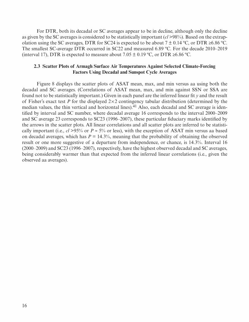
For DTR, both its decadal or SC averages appear to be in decline, although only the decline as given by the SC averages is considered to be statistically important (cl >98%). Based on the extrap-olation using the SC averages, DTR for SC24 is expected to be about 7 ± 0.14 ºC, or DTR ≥6.86 ºC. The smallest SC-average DTR occurred in SC22 and measured 6.89 ºC. For the decade 2010–2019 (interval 17), DTR is expected to measure about 7.05 ± 0.19 ºC, or DTR ≥6.86 ºC.

2.3 Scatter Plots of Armagh Surface Air Temperatures Against Selected Climate-Forcing Factors Using Decadal and Sunspot Cycle Averages

Figure 8 displays the scatter plots of ASAT mean, max, and min versus aa using both the decadal and SC averages. (Correlations of ASAT mean, max, and min against SSN or SSA are found not to be statistically important.) Given in each panel are the inferred linear fit y and the result of Fisher’s exact test P for the displayed 2 × 2 contingency tabular distribution (determined by the median values, the thin vertical and horizontal lines).41 Also, each decadal and SC average is iden-tified by interval and SC number, where decadal average 16 corresponds to the interval 2000–2009 and SC average 23 corresponds to SC23 (1996–2007), these particular fiduciary marks identified by the arrows in the scatter plots. All linear correlations and all scatter plots are inferred to be statisti-cally important (i.e., cl >95% or P ≈ 5% or less), with the exception of ASAT min versus aa based on decadal averages, which has P = 14.3%, meaning that the probability of obtaining the observed result or one more suggestive of a departure from independence, or chance, is 14.3%. Interval 16 (2000–2009) and SC23 (1996–2007), respectively, have the highest observed decadal and SC averages, being considerably warmer than that expected from the inferred linear correlations (i.e., given the observed aa averages).

17

ASAT

Min

imum

(°C)

y

4.5

5

5.5

6.5

7

6

aa10 15 20 25(c)

2000–2009

16 15

1098

36 75

4

1114

1312

y� = 4.4541 � 0.0615xr = 0.623, r2 = 0.388se = 0.33, cl > 98%

5225

� P = 14.3%

ASAT Minimum vs. aa

y

aa10 15 20 25

1996–2007

23

12

1413

20

1718

19

22

2115

1116

y� = 4.3911 � 0.0636xr = 0.656, r2 = 0.43se = 0.31, cl > 98%

7007

� P = 0.029%

ASAT Minimum vs. aa

ASAT

Max

imum

(°C)

y

12

12.5

13

14

13.5

(a)

(b)

(f)

(d)

(e)

2000–200916

1510

836 7 5

9

4

1114

1312

y� = 11.7137 � 0.0565xr = 0.604, r2 = 0.364se = 0.34, cl > 95%

6116

� P = 1.5%

ASAT Maximum vs. aa

ASAT Mean vs. aa ASAT Mean vs. aa

y

y

1996–200723

19

18

13

12

1415

1116

17 22

21

20

y� = 11.7168 � 0.0549xr = 0.621, r2 = 0.386se = 0.29, cl > 98%

6115

� P = 2.5%

ASAT Maximum vs. aa

ASAT

Mea

n (°C

)

y

8.5

9

9.5

10.5

10

2000–200916

1510

8

36 7 5

9

4

1413

1211

y� = 8.0919 � 0.0586xr = 0.633, r2 = 0.4se = 0.33, cl > 98%

6215

� P = 5.1%

Decadal Averages

1996–200723

19

18

13

12

14161511

1722

2120

y� = 8.1122 � 0.0561xr = 0.624, r2 = 0.389se = 0.31, cl > 95%

6115

� P = 2.5%

SC Averages

Figure 8. Decadal (interval) averages of (a) ASAT mean versus aa, (b) ASAT max versus aa, and (c) ASAT min versus aa; SC averages of (d) ASAT mean versus aa, (e) ASAT max versus aa, and (f) ASAT min versus aa.

18

Examination of the scatter plots of Armagh surface air temperatures (mean, max, and min) against aa reveals that the decadal and SC averages of aa can possibly explain about 36%–43% of the variance in the decadal and SC averages of the Armagh surface air temperatures. It is of interest to determine the relationship of Armagh temperatures against other climatic change factors (e.g., NAO, AMO, SOI, and PDO) to determine if they might provide greater explanation for reducing the variance in the Armagh surface air temperatures as compared to using the aa geomagnetic index.

Figure 9 displays the annual and 10-yma values of the NAO and AMO and figure 10 displays the annual and 10-yma values of the SOI and PDO. The NAO describes the difference in surface air pressure between two widely separated locations, in particular Iceland and the subtropical Atlantic Ocean basin (e.g., the Azores, Portugal, or Gilbraltar).83–88 The large-scale, air-mass movements described by the NAO controls the strength and direction of the westerly winds and storm tracks across the North Atlantic Ocean. During the positive phase of the NAO, there is a stronger subtropi-cal high-pressure center and a deeper than usual Icelandic low, while during the negative phase of the NAO, the opposite is true. Values for the NAO index are available online at <http://www.esrl.noaa.gov/psd/gcos_wgsp/Timeseries/Data/nao.long.data> and <http://www.cru.uea.ac.uk~timo/datapages/naoi.htm>.

19

AMO

(°C)

NAO

–0.5

0

0.5 AMO (1856–2012)0.451 (1878)

1850 1900 1950 2000Year

(b)

(a)

mean = 0 °Csd = 0.18 °C

–0.42 (1974)

–2.5

–2

–1.5

–1

–0.5

0

0.5

1

1.5

2 NAO (1843–2012)

1.58 (1868)

mean = 0.07sd = 0.52

–2.19 (2010)

Figure 9. Annual and 10-yma values of (a) NAO for 1843–2012 and (b) AMO for 1856–2012.

20

SOI

–25

–20

–15

–10

–5

0

5

10

15

20

25 SOI (1876–2012)

–20 (1905)

1850 1900 1950 2000

La Niña-Like

Year(b)

mean = 0.12 °Csd = 6.88 °C

20.8 (1917)

PDO

–2

–1.5

–1

–0.5

0

0.5

1

1.5

2

2.5 PDO (1900–2012)

–1.95 (1955)

El Niño-Like

(a)

mean = 0.01sd = 0.77

1.99 (1941)

Figure 10. Annual and 10-yma values of (a) SOI for 1876–2012 and (b) PDO for 1900–2012.

21

The AMO is a fluctuation in the detrended sea surface temperature in the North Atlantic Ocean north of the equator (i.e., 0–70 ºN. latitude).89–100 The AMO has a cycle length of about 65–70 years, fluctuating between warm (positive) and cold (negative) phases, believed to be related to variations in the Atlantic thermohaline circulation (THC), a density-driven, global circulation pat-tern that involves the movement of the warm equatorial surface waters to higher latitudes and the subsequent cooling and sinking of these waters into the deep ocean. The warm phase of the AMO appears to represent intervals of faster THC, while the cold phase of the AMO appears to represent intervals of slower THC. Values of the AMO index are available online at <http://www.esrl.noaa.gov/psd/data/correlation/amon.us.long.data>.

The SOI describes the atmospheric response to anomalous changes in surface air pressure between Tahiti, French Polynesia, and Darwin, Australia, which generally varies inversely with the Oceanic Niño Index (ONI), an index that describes the anomalous changes in the sea surface tem-perature (SST) in the Niño 3.4 region of the Pacific Ocean (located ±5 deg either side of the equator and ±25 deg either side of 145 ºW. longitude). Together, the variations in SOI and ONI are often used to describe the anomalous warming (El Niño) and cooling events (La Niña) associated with the El Niño-Southern Oscillation pattern.101–105 During warm events, the ONI ≥0.5 ºC and the SOI typi-cally is ≤–8 for at least 5 consecutive months, while during cool events the ONI ≤–0.5 ºC and the SOI is typically ≥8 for at least 5 consecutive months. Values of SOI are available online at <http://www.bom.gov.au/climate/current/soihtml.shtml>.

The PDO is defined as the leading principal component of the monthly SST anomalies in the North Pacific Ocean, northward of 20 ºN. The PDO fluctuates between warm (positive) and cool (negative) phases.106–112 During the warm phase, the western Pacific Ocean surface waters become cool and part of the eastern Pacific Ocean surface waters becomes warm, while during the cool phase, the opposite is true. Values of the PDO are available online at <http://jisao.washington.edu/pdo/PDO.latest>.

For the NAO, annually, its values have varied between 1.58 in 1868 to –2.19 in 2010, averaging about 0.07 with sd = 0.52. The –2.19 measured for NAO in 2010 is the most negative value ever seen, being about 4.3 sd lower than the long-term mean. In terms of its 10-yma values, they have varied between about 0.37 in 1909 and –0.42 in 2006.

For the AMO, annually, its values have varied between 0.451 ºC in 1878 and –0.42 ºC in 1974, averaging about 0 ºC with sd = 0.18 ºC. In terms of its 10-yma values, they have varied between –0.25 ºC in 1975 and 0.206 ºC in 2007. The 0.206 ºC measured in 2007 is about 0.037 ºC warmer than the previous peak in 1941 and about 0.102 ºC warmer than the peak of 1876. Warm phases of the AMO (based on 10-yma values in relation to the long-term mean) appear to persist about 35 years in length, while cool phases appear to persist about 30 years in length. The last cool phase was at peak (i.e., most negative 10-yma value) about 1975, with values becoming positive, indicative of the warm phase, about 1995/1996. Thus, the current warm phase, while perhaps having peaked in 2007, is expected to continue (i.e., positive 10-yma values of AMO) for at least another 20 years or so.

22

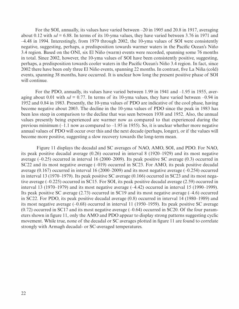
For the SOI, annually, its values have varied between –20 in 1905 and 20.8 in 1917, averaging about 0.12 with sd = 6.88. In terms of its 10-yma values, they have varied between 3.76 in 1971 and –4.48 in 1994. Interestingly, from 1979 through 2002, the 10-yma values of SOI were consistently negative, suggesting, perhaps, a predisposition towards warmer waters in the Pacific Ocean’s Niño 3.4 region. Based on the ONI, six El Niño (warm) events were recorded, spanning some 76 months in total. Since 2002, however, the 10-yma values of SOI have been consistently positive, suggesting, perhaps, a predisposition towards cooler waters in the Pacific Ocean’s Niño 3.4 region. In fact, since 2002 there have been only three El Niño events, spanning 22 months. In contrast, five La Niña (cold) events, spanning 38 months, have occurred. It is unclear how long the present positive phase of SOI will continue.

For the PDO, annually, its values have varied between 1.99 in 1941 and –1.95 in 1955, aver-aging about 0.01 with sd = 0.77. In terms of its 10-yma values, they have varied between –0.94 in 1952 and 0.84 in 1983. Presently, the 10-yma values of PDO are indicative of the cool phase, having become negative about 2003. The decline in the 10-yma values of PDO since the peak in 1983 has been less steep in comparison to the decline that was seen between 1938 and 1952. Also, the annual values presently being experienced are warmer now as compared to that experienced during the previous minimum (–1.1 now as compared to –1.95 in 1955). So, it is unclear whether more negative annual values of PDO will occur over this and the next decade (perhaps, longer), or if the values will become more positive, suggesting a slow recovery towards the long-term mean.

Figure 11 displays the decadal and SC averages of NAO, AMO, SOI, and PDO. For NAO, its peak positive decadal average (0.26) occurred in interval 8 (1920–1929) and its most negative average (–0.25) occurred in interval 16 (2000–2009). Its peak positive SC average (0.3) occurred in SC22 and its most negative average (–019) occurred in SC23. For AMO, its peak positive decadal average (0.167) occurred in interval 16 (2000–2009) and its most negative average (–0.254) occurred in interval 13 (1970–1979). Its peak positive SC average (0.166) occurred in SC23 and its most nega-tive average (–0.225) occurred in SC15. For SOI, its peak positive decadal average (2.59) occurred in interval 13 (1970–1979) and its most negative average (–4.42) occurred in interval 15 (1990–1999). Its peak positive SC average (2.73) occurred in SC19 and its most negative average (–4.6) occurred in SC22. For PDO, its peak positive decadal average (0.8) occurred in interval 14 (1980–1989) and its most negative average (–0.68) occurred in interval 11 (1950–1959). Its peak positive SC average (0.72) occurred in SC17 and its most negative average (–0.64) occurred in SC20. Of the four param-eters shown in figure 11, only the AMO and PDO appear to display strong patterns suggesting cyclic movement. While true, none of the decadal or SC averages plotted in figure 11 are found to correlate strongly with Armagh decadal- or SC-averaged temperatures.

23

PDO

1

0.5

0

–0.5

–1

(d)1850–59

11900–09

61950–59

112000–09

16Decade (Interval)

Decadal Averages SC Averages

0.8

–0.68

108 12 14 16 18 20 22 24Sunspot Cycle

0.72

–0.64

SOI

5

0

–5

(a)

(b)

(c)

(h)

(e)

(f)

(g)

2.59

–4.42

2.73

–4.6

AMO

(°C)

0

0.3

–0.3

0.167

–0.254 –0.225

NAO 0

0.3

–0.3

0.26

–0.25

0.3

–0.19

–0.166

Figure 11. Decadal (interval) averages of (a) NAO, (b) AMO, (c) SOI, and (d) PDO; SC averages of (e) NAO, (f) AMO, (g) SOI, and (h) PDO.

Figure 12 displays another parameter that strongly relates to climatic change—the MLCO2 index. The MLCO2 is a measure of the atmospheric concentration of CO2 as measured at the Mauna Loa Observatory on the Big Island of Hawaii.113–120 The Observatory is located on the northern slope of the volcano Mauna Loa at an elevation of 3,400 m above sea level and 800 m below its sum-mit. Annual means of MLCO2 (in units of ppm) are available on line at <ftp://ftp.cmdl.noaa.gov/ccg/co2/trends/co2_annmean_mlo.txt>.

24

MLCO

2 (pp

m)

MLCO

2 (pp

m)

MLCO

2 (pp

m)

300

325

350

350

375

400

(c) 108

1850 1900 1950 2000

12 14 16 18 20 22 24Sunspot Cycle

MLCO2 (1959–2012)

300

325

375

400

(b)

350

300

325

375

400

(a)

1850–591

1900–096

1950–5911

2000–0916

Decade (Interval)

Year

Figure 12. MLCO2: (a) Annual values for 1959–2012, (b) decadal (interval) averages, and (c) SC averages.

25

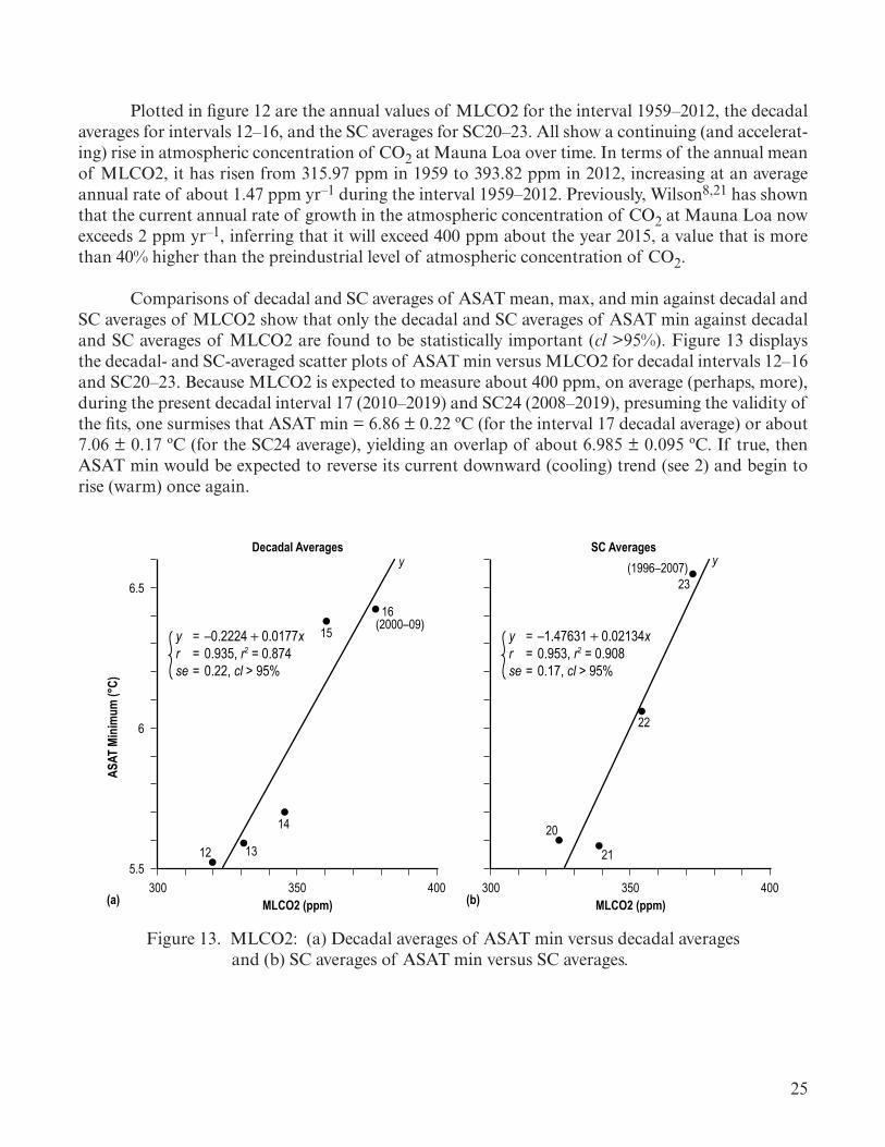
Plotted in figure 12 are the annual values of MLCO2 for the interval 1959–2012, the decadal averages for intervals 12–16, and the SC averages for SC20–23. All show a continuing (and accelerat-ing) rise in atmospheric concentration of CO2 at Mauna Loa over time. In terms of the annual mean of MLCO2, it has risen from 315.97 ppm in 1959 to 393.82 ppm in 2012, increasing at an average annual rate of about 1.47 ppm yr–1 during the interval 1959–2012. Previously, Wilson8,21 has shown that the current annual rate of growth in the atmospheric concentration of CO2 at Mauna Loa now exceeds 2 ppm yr–1, inferring that it will exceed 400 ppm about the year 2015, a value that is more than 40% higher than the preindustrial level of atmospheric concentration of CO2.

Comparisons of decadal and SC averages of ASAT mean, max, and min against decadal and SC averages of MLCO2 show that only the decadal and SC averages of ASAT min against decadal and SC averages of MLCO2 are found to be statistically important (cl >95%). Figure 13 displays the decadal- and SC-averaged scatter plots of ASAT min versus MLCO2 for decadal intervals 12–16 and SC20–23. Because MLCO2 is expected to measure about 400 ppm, on average (perhaps, more), during the present decadal interval 17 (2010–2019) and SC24 (2008–2019), presuming the validity of the fits, one surmises that ASAT min = 6.86 ± 0.22 ºC (for the interval 17 decadal average) or about 7.06 ± 0.17 ºC (for the SC24 average), yielding an overlap of about 6.985 ± 0.095 ºC. If true, then ASAT min would be expected to reverse its current downward (cooling) trend (see 2) and begin to rise (warm) once again.

ASAT

Min

imum

(°C)

5.5

6

6.5

(a) (b)300 350

1516

14

1312

400MLCO2 (ppm)

Decadal Averagesy

y� = –0.2224 � 0.0177xr = 0.935, r2 = 0.874se = 0.22, cl > 95%

300 350

23(1996–2007)

(2000–09)

22

21

20

400MLCO2 (ppm)

SC Averagesy

y� = –1.47631 � 0.02134xr = 0.953, r2 = 0.908se = 0.17, cl > 95%

Figure 13. MLCO2: (a) Decadal averages of ASAT min versus decadal averages and (b) SC averages of ASAT min versus SC averages.

26

Table 2 gives the inferred regressions and statistics (where a is the y-intercept, b is the slope, t is the t statistic for the slope, and n is the sample size) using both decadal and SC averages of ASAT mean, max, and min against SSN, aa, SSA, NAO, AMO, SOI, PDO, and MLCO2. For comparison, the sd and mean value are given for the y parameters (i.e., ASAT mean, max, and min). As previ-ously noted, based on linear regression analysis, the only inferred regressions found to be statistically important (cl >95%) are those against aa (ASAT mean, max, and min) and MLCO2 (ASAT min).

Table 2. Inferred regressions of y versus x using decadal averages and SC averages.

Parameter yDecadal Averages SC Averages

Parameter x Statistic ASAT Mean ASAT Max ASAT Min ASAT Mean ASAT Max ASAT MinSSN a 8.7283 12.4076 5.0495 8.7317 12.3529 5.060

b 0.0093 0.0078 0.0107 0.0088 0.0085 0.010r 0.416 0.338 0.453 0.470 0.445 0.502

rxr 0.173 0.114 0.205 0.221 0.198 0.252se 0.336 0.397 0.359 0.350 0.338 0.404sd 0.372 0.386 0.393 0.352 0.358 0.378

mean 9.239 12.838 5.638 9.233 12.836 5.635n 16 16 16 15 15 15t 1.784 1.266 1.921 1.763 1.763 1.737cl >90% <90% >90% <90% <90% <90%

aa a 8.0919 11.7137 4.4541 8.1122 11.7168 4.3911b 0.0586 0.0565 0.0615 0.0561 0.0549 0.0636r 0.633 0.604 0.623 0.624 0.621 0.656

rxr 0.400 0.364 0.388 0.389 0.386 0.430se 0.329 0.343 0.332 0.313 0.288 0.313sd 0.391 0.396 0.417 0.378 0.371 0.407

mean 9.235 12.816 5.652 9.222 12.802 5.648n 14 14 14 13 13 13t 2.71 2.507 2.822 2.604 2.769 2.953cl >98% >95% >98% >95% >98% >98%

SSA a 8.7289 12.2765 5.11238 8.72740 12.31425 5.10213b 0.0006 0.0006 0.00065 0.00057 0.00056 0.00063r 0.457 0.407 0.443 0.471 0.476 0.480

rxr 0.209 0.166 0.196 0.222 0.226 0.231se 0.549 0.502 0.400 0.370 0.436 0.374sd 0.386 0.384 0.419 0.392 0.384 0.423

mean 9.268 12.854 5.681 9.234 12.816 5.660n 13 13 13 12 12 12t 1.079 1.180 1.605 1.650 1.376 1.806cl <90% <90% <90% <90% <90% <90%

NAO a 9.3101 12.9170 5.7066 9.3352 12.9321 5.7255b –0.8503 –0.9486 –0.8243 –1.0051 –0.9484 –0.8896r –0.349 –0.375 –0.320 –0.369 –0.342 –0.303

rxr 0.122 0.141 0.102 0.136 0.117 0.092se 0.360 0.370 0.386 0.339 0.349 0.374sd 0.372 0.386 0.393 0.352 0.358 0.378

mean 9.239 12.838 5.638 9.233 12.836 5.635n 16 16 16 15 15 15t –1,395 –1.517 –1.262 –1.430 –1.311 –1.149cl <90% <90% <90% <90% <90% <90%

27

Parameter yDecadal Averages SC Averages

Parameter x Statistic ASAT Mean ASAT Max ASAT Min ASAT Mean ASAT Max ASAT MinAMO a 9.2298 12.8167 5.6405 9.2288 12.8177 5.6445

b 0.9105 1.0521 0.8073 0.8694 0.9128 0.7620r 0.320 0.368 0.265 0.322 0.343 0.261

rxr 0.102 0.135 0.070 0.104 0.118 0.068se 0.374 0.369 0.407 0.358 0.350 0.394sd 0.380 0.382 0.407 0.363 0.358 0.392

mean 9.224 12.810 5.635 9.223 12.811 5.639n 15 15 15 14 14 14t 1.217 1.423 0.990 1.179 1.266 0.938cl <90% <90% <90% <90% <90% <90%

SOI a 9.2652 12.8514 5.6766 9.2326 12.8148 5.6567b –0.0462 –0.0344 –0.0578 –0.0261 –0.0163 –0.0541r –0.249 –0.186 –0.286 –0.144 –0.093 –0.278

rxr 0.062 0.035 0.082 0.021 0.009 0.077se 0.390 0.394 0.420 0.406 0.402 0.426sd 0.386 0.384 0.419 0.392 0.384 0.423

mean 9.268 12.854 5.681 9.234 12.816 6.660n 13 13 13 12 12 12t –0.852 –0.628 –0.990 –0.463 –0.292 –0.915cl <90% <90% <90% <90% <90% <90%

PDO a 9.3593 12.9302 5.7876 9.3397 12.9115 5.7777b 0.0224 –0.0622 0.0997 –0.0351 –0.1128 0.0879r 0.030 –0.078 0.128 –0.057 –0.179 0.136

rxr 0.001 0.006 0.016 0.003 0.032 0.019se 0.352 0.374 0.363 0.337 0.339 0.349sd 0.335 0.356 0.347 0.318 0.324 0.332

mean 9.360 12.928 5.791 9.338 12.906 5.782n 11 11 11 10 10 10t 0.089 –0.234 0.385 –0.161 –0.515 0.390cl <90% <90% <90% <90% <90% <90%

MLC02 a 3.6064 7.2542 –0.2224 3.14464 7.40545 –1.47631b 0.0169 0.0167 0.0177 0.01818 0.01618 0.02134r 0.955 0.893 0.935 0.866 0.805 0.953

rxr 0.911 0.798 0.874 0.751 0.648 0.908se 0.478 0.473 0.217 0.292 0.213 0.170sd 0.412 0.436 0.441 0.430 0.412 0.459

mean 9.486 13.058 5.922 9.470 13.033 5.948n 5 5 5 4 4 4t 1.640 1.646 3.802 2.208 2.696 4.448cl <90% <90% >95% <90% <90% >95%

Table 2. Inferred regressions of y versus x using decadal averages and SC averages (Continued).

28

2.4 Multivariate Fits

Table 3 gives the inferred regressions and statistics (both for decadal averages and SC aver-ages) using multivariate fits for ASAT mean, max, and min against aa and MLCO2 in combination with each other and in combination with NAO, AMO, SOI, and PDO, ordered by the inferred coef-ficient of determination (r2). In table 3, Sy12 is the standard error of the estimate for parameter y based on parameters 1 and 2, Ry12 is the sample multiple correlation coefficient, R2

y12 sample coef-ficient of multiple determination for parameter y based on parameters 1 and 2, sy is the standard deviation for parameter y and n is the sample size. The strongest inferred multivariate regressions are those that incorporate combinations with MLCO2.

Table 3. Results of multivariate fitting.

Decadal AveragesInferred Multivariate Fit Sy12 Ry12 (rxr)12 sy n

ASAT mean (predicted) = 4.7642 – 0.0499aa + 0.0169MLCO2 0.103 0.984 0.969 0.412 5= 4.9579 + 0.8432AMO + 0.0132MLCO2 0.105 0.984 0.967 0.412 5= 2.9942 – 0.1826PDO + 0.0187MLCO2 0.115 0.980 0.961 0.412 5= 3.8364 – 0.3042NAO + 0.0163MLCO2 0.161 0.957 0.915 0.412 5= 3.5331 + 0.0050SOI + 0.0172MLCO2 0.173 0.955 0.912 0.412 5= 8.1679 + 0.0552aa + 0.7538AMO 0.310 0.684 0.468 0.391 14= 8.2082 + 0.0549aa – 0.5673NAO 0.315 0.673 0.454 0.391 14= 8.2290 + 0.0523aa – 0.0236SOI 0.337 0.603 0.363 0.386 13= 8.5219 + 0.0408aa + 0.0692PDO 0.321 0.513 0.263 0.335 11

ASAT max (predicted) = 9.4934 – 0.0981aa + 0.0167MLCO2 0.043 0.998 0.995 0.436 5= 8.0699 – 1.1338NAO + 0.0143MLCO2 0.129 0.978 0.956 0.436 5= 9.4387 + 1.3878AMO + 0.0106MLCO2 0.158 0.966 0.934 0.436 5= 6.2105 – 0.3002PDO + 0.0197MLCO2 0.172 0.951 0.905 0.436 5= 6.5504 + 0.0421SOI + 0.0188MLCO2 0.234 0.925 0.856 0.436 5= 11.8028 + 0.0525aa + 0.8845AMO 0.317 0.675 0.456 0.396 14= 11.8554 + 0.0520aa – 0.6900NAO 0.321 0.664 0.441 0.396 14= 11.8692 + 0.0495aa – 0.0130SOI 0.350 0.555 0.309 0.384 13= 12.1238 + 0.0393aa – 0.0169PDO 0.351 0.471 0.222 0.356 11

ASAT min (predicted) = 0.1705 – 0.0267SOI + 0.0165MLCO2 0.201 0.947 0.896 0.441 5= –0.5667 + 0.4211NAO + 0.0187MLCO2 0.202 0.946 0.895 0.441 5= –0.5678 – 0.0939PDO + 0.0187MLCO2 0.210 0.941 0.886 0.441 5= 0.3531 + 0.3764AMO + 0.0161MLCO2 0.213 0.940 0.884 0.441 5= –0.0252 – 0.0098aa + 0.0178MLCO2 0.220 0.936 0.876 0.441 5= 4.5209 + 0.0585aa + 0.6633AMO 0.341 0.659 0.434 0.417 14= 4.5600 + 0.0581aa – 9.5156NAO 0.343 0.653 0.427 0.417 14= 4.5681 + 0.0559aa – 0.0335SOI 0.363 0.612 0.374 0.419 13= 4.9082 + 0.0429aa + 0.1488PDO 0.328 0.534 0.286 0.347 11

SC AveragesASAT mean (predicted) = 4.8433 – 0.0923aa + 0.0195MLCO2 0.064 0.996 0.993 0.430 4

= 11.9386 + 3.3703AMO – 0.0064MLCO2 0.090 0.993 0.985 0.430 4= 3.6522 – 0.8432NAO + 0.0168MLCO2 0.223 0.954 0.910 0.430 4= 1.0434 – 0.4431PDO + 0.0244MLCO2 0.294 0.919 0.834 0.430 4= 1.6502 + 0.0719SOI + 0.0228MLCO2 0.364 0.872 0.761 0.430 4= 8.2621 + 0.0526aa – 0.7649NAO 0.302 0.684 0.467 0.378 13= 8.1712 + 0.0535aa + 0.6980AMO 0.306 0.674 0.454 0.378 13= 8.0374 + 0.0600aa + 0.0202SOI 0.338 0.626 0.391 0.392 12= 8.6093 + 0.0353aa – 0.2116PDO 0.317 0.475 0.226 0.319 10

29

SC AveragesInferred Multivariate Fit Sy12 Ry12 (rxr)12 sy n

ASAT max (predicted) = 5.7131 + 0.0815SOI + 0.0214MLCO2 0.044 0.998 0.996 0.412 4= 5.0020 – 0.5072PDO + 0.0233MLCO2 0.045 0.998 0.996 0.412 4= 17.2651 + 3.7792AMO – 0.0114MLCO2 0.122 0.985 0.971 0.412 4= 7.9579 – 0.9213NAO + 0.0147MLCO2 0.270 0.926 0.857 0.412 4= 10.1487 – 0.0178aa + 0.0095MLCO2 0.311 0.900 0.809 0.412 4= 11.7773 + 0.0522aa + 0.7160AMO 0.299 0.676 0.457 0.371 13= 11.8504 + 0.0517aa – 0.6811NAO 0.301 0.671 0.450 0.371 13= 11.6115 + 0.0604aa + 0.0302SOI 0.345 0.581 0.338 0.384 12= 12.1245 + 0.0376aa – 0.0980PDO 0.317 0.506 0.256 0.324 10

ASAT min (predicted) = –2.7867 – 0.2764PDO + 0.0252MLCO2 0.081 0.995 0.990 0.459 4= –2.3130 + 0.0404SOI + 0.0239MLCO2 0.122 0.988 0.977 0.459 4= –0.5820 – 0.0485aa + 0.0220MLCO2 0.145 0.983 0.967 0.459 4= 2.9507 + 1.6976AMO + 0.0090MLCO2 0.157 0.980 0.961 0.459 4= –1.2941 – 0.3008NAO + 0.0208MLCO2 0.217 0.962 0.926 0.459 4= 4.5178 + 0.0606aa – 0.6461NAO 0.322 0.691 0.478 0.407 13= 4.4414 + 0.0614aa + 0.5970AMO 0.325 0.686 0.471 0.407 13= 4.4081 + 0.0626aa – 0.0059SOI 0.355 0.651 0.424 0.422 12= 4.9372 + 0.0401aa + 0.1037PDO 0.324 0.512 0.262 0.332 10

As an example, comparing decadal averages of ASAT mean against decadal averages of aa and MLCO2 provides the greatest explanation for reducing the variance, from 40% to 97% as com-pared to using aa alone or from 91% to 97% as compared to using MLCO2 alone. Hence, it appears that one can estimate the decadal average of ASAT mean from the inferred multivariate regression based on estimations for the decadal averages of the aa-geomagnetic index and MLCO2; i.e., y = 4.8096 – 0.0506aa + 0.0168MLCO2, having r = 0.983 and se = 0.106. Comparing SC averages of ASAT mean against SC averages of aa and MLCO2, likewise, provides the greatest explanation for reducing the variance, from 39% to 99% as compared to using aa alone or from 75% to 99% as com-pared to using MLCO2 alone.

Figure 14 compares the observed decadal and SC averages of ASAT mean, max, and min with the inferred decadal and SC averages of ASAT mean, max, and min as given by the best multi-variate fits. The diagonal line in each panel is simply the 1:1 line for comparison. When the plotted value lies above the line, this means that the observed value is slightly higher than the predicted value, while when the plotted value lies below the line, it means the observed value is slightly lower than the predicted value. For both decadal and SC averages, the worst fit is for ASAT min (Ry12 = 0.95, Sy12 = 0.202 and Ry12 = 0.995, Sy12 = 0.081, respectively), although all fits generally have observed minus predicted values within the ±1 Sy12 prediction interval.

Table 3. Results of multivariate fitting (Continued).

30

ASAT

Min

imum

(Obs

erve

d)

5

6

5.5

7

6.5

(c)5 5.5 6 6.5

Ry12 = 0.947Sy12 = 0.201

7

1516

141312

ASAT Minimum (SOI, MLCO2)5 5.5 6 6.5

Ry12 = 0.995Sy12 = 0.081

7

23

2120

22

ASAT Minimum (PDO, MLCO2)

ASAT

Max

imum

(Obs

erve

d)

12

13

12.5

14

13.5

(b)

(a)

(f)

(e)

(d)

12 12.5 13 13.5

Ry12 = 0.998Sy12 = 0.043

14 12 12.5 13 13.5 14

15

16

14

13

12

ASAT Maximum (aa, MLCO2)

Ry12 = 0.998Sy12 = 0.044

23

21

2022

ASAT Maximum (SOI, MLCO2)

ASAT Mean (aa, MLCO2) ASAT Mean (aa, MLCO2)

Decadal Averages SC Averages

ASAT

Mea

n (O

bser

ved)

9

10

9.5

10.5

9 9.5 10 10.5 9 9.5 10 10.5

Ry12 = 0.984Sy12 = 0.103

15

16

1413

12Ry12 = 0.996Sy12 = 0.064

23

21

2022

Figure 14. Decadal averages of (a) ASAT mean versus ASAT mean (aa, MLCO2), (b) ASAT max versus ASAT max (aa, MLCO2), and (c) ASAT min versus ASAT min (SOI, MLCO2); SC averages of (d) ASAT mean versus ASAT mean (aa, MLCO2), (e) ASAT max versus ASAT max (SOI, MLCO2), and (f) ASAT min versus ASAT min (PDO, MLCO2).

31

From figure 14, it is apparent that if one had good estimates for the expected values of the x1 and x2 parameters, it might be possible to better predict ASAT mean, max, and min for both inter-val 17 (2010–2019) and SC24 than by simply using the inferred linear or mean fits. To accomplish this, one can determine the distributions of the first differences (fd) of the decadal and SC averages for each parameter, add the suggested parametric values to the last known values (interval 16 and SC23) to obtain parametric estimates for interval 17 or SC24, and then use these estimates in the inferred multivariate regressions to estimate ASAT mean, max, and min for interval 17 (2010–2019) and SC24. Table 4 lists the fds of the decadal and SC averages for ASAT mean, max, and min, as well as for aa, NAO, AMO, SOI, PDO, and MLCO2, and figures 15 and 16 display temporal plots of the parametric fds. Now, a positive fd means a larger parametric value for the following interval or SC, while a negative fd means a smaller parametric value for the following interval or SC. Because fd(MLCO2) appears to be growing faster from one interval or SC to the next, this suggests that the overall trend in ASAT mean, max, and min probably will tend to be upward over time, being modu-lated by the other climatic forcing factors.

Table 4. First differences of parametric decadal and SC averages.

Decadal AveragesASAT

Interval mean max min aa NAO AMO SOI PDO MLCO201–02 –0.40 –0.53 –0.28 – 0.12 – – – –02–03 –0.27 –0.41 –0.12 – –0.41 0.023 – – –03–04 –0.22 –0.11 –0.34 1.4 0.46 –0.042 – – –04–05 0.37 0.47 0.27 0.7 – –0.071 0.53 – –05–06 0.02 –0.19 0.22 –4.6 –0.01 –0.109 0.02 – –06–07 0.05 0.15 –0.03 3.8 –0.07 –0.084 0.31 –0.29 –07–08 0.15 0.05 0.24 – 0.11 0.066 2.04 0.19 –08–09 0.17 0.18 0.17 3.2 –0.21 0.004 –0.47 0.27 –09–10 0.25 0.33 0.16 3.3 0.05 –0.045 –4.22 –0.24 –10–11 –0.15 –0.17 –0.13 2.6 0.01 0.029 4.89 –0.86 –11–12 –0.27 –0.21 –0.32 –4.2 –0.16 –0.137 –2.14 0.14 –12–13 –0.02 –0.11 0.07 2.3 0.08 –0.246 2.34 0.13 10.5513–14 0.13 0.16 0.11 1.9 0.03 0.141 –4.87 1.21 14.6714–15 0.47 0.27 0.68 –0.8 0.12 0.104 –2.14 –0.46 14.9215–16 0.33 0.67 0.04 –3.5 –0.43 0.176 4.45 –0.45 18.13mean 0.04 0.04 0.05 0.5 –0.02 –0.014 0.06 –0.04 14.57

sd 0.26 0.33 0.27 2.9 0.22 0.115 3.08 0.57 3.11SC Averages

ASATSC mean max min aa NAO AMO SOI PDO MLCO2

09–10 –0.14 –0.24 –0.05 – 0.03 – – – –10–11 –0.17 –0.31 –0.03 – –0.01 0.021 – – –11–12 –0.61 –0.57 –0.65 –2.4 –0.06 0.013 – – –12–13 0.51 0.61 0.40 0.9 0.22 –0.074 –1.00 – –13–14 0.02 –0.14 0.19 –2.6 –0.02 –0.180 0.66 – –14–15 0.13 0.19 0.07 4.0 –0.01 –0.057 1.24 –0.31 –15–16 –0.06 –0.17 0.06 0.1 –0.11 0.214 –0.42 0.48 –16–17 0.37 0.44 0.09 3.1 –0.11 0.138 –1.49 0.39 –17–18 0.08 0.15 0.02 2.9 0.22 0.011 0.59 –1.33 –18–19 –0.12 –0.14 –0.11 1.4 –0.13 –0.043 2.47 0.03 –19–20 –0.13 –0.10 –0.17 –3.5 –0.14 –0.278 0.10 –0.06 –20–21 –0.14 –0.24 –0.02 3.8 0.10 0.014 –6.16 1.18 14.0921–22 0.29 0.29 0.48 1.0 0.25 0.080 –1.17 0.01 15.2322–23 0.68 0.67 0.49 –4.0 –0.49 0.255 3.87 –0.38 18.40mean 0.05 0.03 0.06 0.4 –0.02 0.009 –0.12 – 15.91

sd 0.33 0.37 0.29 2.9 0.19 0.146 2.57 0.69 2.23

32

fd(A

SAT

Mini

mum

)

–0.5

–1

0

0.5

1

(f) 108 12 14 16 18 20 22SC

mean = 0.06 °Csd = 0.29 °C

fd(A

SAT

Maxim

um)

–0.5

0

0.5

1

(e)

(d)

fd(A

SAT

Mini

mum

)

–0.5

0

0.5

1

(c) 20 4 6 8 10 12 14 16Interval

Decadal Averages SC Averages

mean = 0.05 °Csd = 0.27 °C

(b)

fd(A

SAT

Maxim

um)

–0.5

–1

–1

–1

–1

0

0.5

1

mean = 0.04 °Csd = 0.33 °C

(a)

fd(A

SAT

Mean

)0

0.5

–0.5

mean = 0.04 °Csd = 0.26 °C

mean = 0.03 °Csd = 0.37 °C

fd(A

SAT

Maxim

um)

–0.5

0

0.5

1

mean = 0.05 °Csd = 0.33 °C

Figure 15. First difference (fd) values based on decadal (interval) averages of (a) ASAT mean, (b) ASAT max, and (c) ASAT min; fd values based on SC averages of (d) ASAT mean, (e) ASAT max, and (f) ASAT min.

33

(l) 108 12 14 16 18 20 22SC

mean = 15.91 ppmsd = 2.23 ppm

mean = 0.12 °Csd = 2.57 °C

mean = 0sd = 0.69

mean = –0.04sd = 0.57

fd(M

LCO2

)fd

(PDO

)fd

(SOI

)fd

(AMO

)fd

(NAO

)fd

(aa)

25

2

5

0

–5

0

–2

20

15

10(f)

(k)(e)

(j)(d)

(i)(c)

(h)(b)

(g)(a)

20 4 6 8 10 12 14 16Interval

SC AveragesDecadal Averages

mean = 14.57 ppmsd = 3.11 ppm

mean = 0.009 °Csd = 0.146 °C

mean = –0.02 °Csd = 0.19 °C

mean = 0.4sd = 2.9

mean = –0.02sd = 0.22

mean = 0.06sd = 3.08

0.5–0.5

0

mean = 0.5sd = 2.9

0.5

0

5

–5

0

–0.5

mean = –0.014 °Csd = 0.115 °C

Figure 16. First difference (fd) values based on decadal (interval) averages of (a) aa, (b) NAO, (c) AMO, (d) SOI, (e) PDO, and (f) MLCO2; fd values based on SC averages of (g) aa, (h) NAO, (i) AMO, (j) SOI, (k) PDO, and (l) MLCO2.

34

From figure 15, one finds that, based on the decadal averages, fd(ASAT mean) = 0.04 ± 0.26 ºC (i.e., the mean ±1 sd prediction interval), fd(ASAT max) = 0.04 ± 0.33 ºC and fd(ASAT min) = 0.05 ± 0.27 ºC and, based on the SC averages, fd(ASAT mean) = 0.05 ± 0.33 ºC, fd(ASAT max) = 0.03 ± 0.37 ºC, and fd(ASAT min) = 0.06 ± 0.29 ºC. Adding these values to the last known values of interval 16 and SC23 yields estimates for interval 17 and SC24; namely, ASAT mean, max, and min equal to 10.12 ± 0.26, 13.83 ± 0.33, and 6.47 ± 0.27 ºC, respectively, for interval 17 based on decadal averages and ASAT mean, max, and min equal to 10.14 ± 0.33, 13.65 ± 0.37, and 6.61 ± 0.29 ºC, respectively, for SC24 based on SC averages.

Alternately, one can infer estimates for ASAT mean, max, and min using the inferred multi-variate regressions. Table 5 presents decadal and SC estimates for ASAT mean, max, and min based on the inferred multivariate regressions that use combinations coupled with MLCO2. Interval 17 and SC24 parametric values, except for MLCO2, are determined by adding the fd means and sd values as applied to the last known interval (16) and SC (23) parametric values. For the MLCO2 parametric value, linear regression analysis (not shown) suggests that fd(MLCO2) should be about 20.15 ± 1.05 for interval 16 and about 20.22 ± 0.82 for SC23, inferring that MLCO2 will measure about 398.71 ± 1.05 ppm for interval 17 (2010–2019) and about 393.04 ± 0.82 ppm for SC24. In the computations for decadal and SC averages of ASAT mean, max, and min, it is these values, respectively, that are used for MLCO2.

35

Table 5. Estimates of ASAT mean, max, and min for interval 17 (2010–2019) and SC24 using the inferred multivariate fits in conjunction with last known parametric values and the means of the parametric fd values, except for MLCO2.

Decadal Averages

Method x1 Value x2 Value

ASAT Value

(Predicted) Sy12 Ry12ASAT mean = 4.76 – 0.050aa + 0.017MLCO2 21.3(2.9) 398.71(1.05) 10.47 0.10 0.984

= 4.96 + 0.843AMO + 0.013MLCO2 0.153(0.115) 398.71(1.05) 10.26 0.11 0.984= 2.99 – 0.183PDO + 0.019MLCO2 –0.15(0.57) 398.71(1.05) 10.58 0.11 0.980= 3.84 – 0.304NAO + 0.016MLCO2 –0.27(0.22) 398.71(1.05) 10.30 0.16 0.957= 3.53 + 0.005SOI + 0.017MLCO2 0.09(3.08) 398.71(1.05) 10.31 0.17 0.955

ASAT max = 9.49 – 0.098aa + 0.017MLCO2 21.3(2.9) 398.71(1.05) 14.18 0.04 0.998= 8.07 – 1.13NAO + 0.014MLCO2 –0.27(0.22) 398.71(1.05) 13.96 0.13 0.978= 9.44 + 1.39AMO + 0.011MLCO2 0.153(0.115) 398.71(1.05) 14.04 0.16 0.966= 6.21 – 0.30PDO + 0.020MLCO2 –0.15(0.57) 398.71(1.05) 14.23 0.17 0.951= 6.55 + 0.04SOI + 0.019MLCO2 0.09(3.08) 398.71(1.05) 14.13 0.23 0.925

ASAT min = 0.17 – 0.03SOI + 0.017MLCO2 0.09(3.08) 398.71(1.05) 6.95 0.20 0.947= –0.57 + 0.42NAO + 0.019MLCO2 –0.27(0.22) 398.71(1.05) 6.89 0.20 0.946= –0.57 – 0.09PDO + 0.019MLCO2 –0.15(0.57) 398.71(1.05) 7.02 0.21 0.941= 0.35 + 0.38AMO + 0.016MLCO2 0.153(0.115) 398.71(1.05) 6.79 0.21 0.940= –0.03 – 0.01aa + 0.018MLCO2 21.3(2.9) 398.71(1.05) 6.93 0.22 0.936

SC AveragesASAT mean = 4.84 – 0.09aa + 0.020MLCO2 22.3(2.9) 393.04(0.82) 10.69 0.06 0.996

= 11.94 + 3.37AMO – 0.006MLCO2 0.175(0.146) 393.04(0.82) 10.17 0.09 0.993= 3.65 – 0.84NAO + 0.017MLCO2 –0.21(0.19) 393.04(0.82) 10.51 0.22 0.954= 1.04 – 0.44PDO + 0.024MLCO2 0.17(0.69) 393.04(0.82) 10.40 0.29 0.919= 1.65 + 0.07SOI + 0.023MLCO2 –0.61(2.57) 393.04(0.82) 10.65 0.36 0.872

ASAT max = 5.71 + 0.08SOI + 0.021MLCO2 –0.61(2.57) 393.04(0.82) 13.92 0.04 0.998= 5.00 – 0.51PDO + 0.023MLCO2 0.17(0.69) 393.04(0.82) 13.95 0.05 0.998= 17.27 + 3.78AMO – 0.011MLCO2 0.175(0.146) 393.04(0.82) 13.61 0.12 0.985= 7.96 – 0.92NAO + 0.015MLCO2 –0.21(0.19) 393.04(0.82) 14.05 0.27 0.926= 10.15 – 0.02aa + 0.010MLCO2 22.3(2.9) 393.04(0.82) 13.63 0.31 0.900

ASAT min = –2.79 – 0.28PDO + 0.025MLCO2 0.17(0.69) 393.04(0.82) 6.99 0.08 0.995= –2.31 + 0.04SOI + 0.024MLCO2 –0.61(2.57) 393.04(0.82) 7.10 0.12 0.988= –0.58 – 0.05aa + 0.022MLCO2 22.3(2.9) 393.04(0.82) 6.95 0.15 0.983= 2.95 + 1.70AMO + 0.009MLCO2 0.175(0.146) 393.04(0.82) 6.78 0.16 0.980= –1.29 – 0.30NAO + 0.021MLCO2 –0.21(0.19) 393.04(0.82) 7.03 0.22 0.962

From table 5, one finds that, presuming the validity of the inferred multivariate regressions and the accuracy of the expected x1 and x2 parametric values, the decadal average of ASAT mean for the current decade (interval 17, 2010–2019) is anticipated to be about 10.38 ± 0.14 ºC, determined by averaging the five individual predicted values. The lowest value measures 10.26 ºC based on the multivariate fit employing AMO and MLCO2, while the highest value measures 10.58 ºC based on the multivariate fit employing PDO and MLCO2. It should be noted that all predictions of ASAT mean from the multivariate regressions suggest that, for the current interval 17 (2010–2019), it will be warmer than was seen during any previous decade. Hence, a new record high seems likely at Armagh. If MLCO2 actually measures higher than the estimated 398.71 ppm for the current decade, then this would suggest an even higher temperature at Armagh. Likewise, positive values of AMO and SOI, which are indicative of warming in the Atlantic and cooling in the Pacific Niño 3.4 region,

36

also would be suggestive of somewhat higher temperatures at Armagh. On the other hand, a higher value of aa and/or positive values of PDO and NAO would suggest slightly lower temperatures at Armagh. Unfortunately, the current trend based on 10-yma values (see figs. 4, 9, 10, and 12) for all parameters is for higher MLCO2, lower aa, positive AMO, negative NAO, positive SOI, and negative PDO, these trends being highly suggestive of warmer temperatures at Armagh during the present decade. (Showstack121 has noted that the year 2012 was one of the 10 warmest years on record; see the summary report122 “State of the climate in 2012.” Also, Compo et al.123 have recently reported an independent confirmation of global land warming, inferred from observations of barometric pressure, sea surface temperature, and sea ice concentration using a physically based data assimila-tion system called the ‘20th Century Reanalysis.’)

For ASAT max and ASAT min, respectively, the averages are 14.11 ± 0.11 ºC and 6.92 ± 0.08 ºC, these values also being of record warmth, higher than for any previous decade. Accepting these values, one estimates the decadal DTR for interval 17 (2010–2019) to be about 7.19 ± 0.07 ºC, a value slightly higher than was seen in interval 16 (2000–2009), which measured 7.07 ± 0.46 ºC.

Based on SC averages, one estimates ASAT mean, max, and min, respectively, to be 10.48 ± 0.21, 13.83 ± 0.20, and 6.97 ± 0.12 ºC for SC24. In comparison, SC23 had ASAT mean, max, and min, respectively, equal to 10.09 ± 0.37, 13.62 ± 0.49, and 6.55 ± 0.38 ºC. Hence, based on this analy-sis, it appears that SC-averaged temperatures for SC24 could possibly be higher than was seen for SC23, in contrast to the prediction of Solheim et al.83,84

Table 6 provides a comparison of decadal and SC parametric averages for intervals 16 (2000–2009) and 17 (2010–present) and SC23 (1996–2007) and 24 (2008–present). For the average of the first 3 years of the decade, ASAT min, max, and mean have each been of higher average value for interval 16 (the previous decade) than for interval 17 (the present decade), while the DTR has been of smaller average value for interval 16 than for interval 17. The average values for the first 3 years of the decade for aa, NAO, AMO, SOI, PDO, and MLCO2 have been, respectively, higher, higher, lower, lower, higher, and lower for interval 16 than for interval 17. For the average of the first 5 years of the SC, ASAT min, max, and mean have been, respectively, higher, lower, and higher for SC23 than for SC24, and the DTR has been lower for SC23 than for SC24. The average values for the first 5 years of the sunspot cycle for aa, NAO, AMO, SOI, PDO, and MLCO2 have been, respectively, higher, higher, lower, lower, higher, and lower for SC23 than for SC24. Thus, the current values of the climate-forcing parameters are supportive for continued warming during interval 17 (the present decade, 2010–2019) and SC24 (2008–present).

37

Table 6. Comparison of decadal and SC parametric values for intervals 16 (2000–2009) and 17 (2010–2019), and SC23 (1996–2007) and 24 (2008–present).

A. Decadal ValuesInterval 16 (2000–2009)

ASATt min max mean DTR aa NAO AMO SOI PDO MLCO20 6.37 13.49 9.93 7.12 25.4 0.04 0.040 7.8 –0.59 369.521 5.95 13.19 9.57 7.24 22.4 –0.45 0.135 0.5 –0.56 371.132 6.78 13.62 10.20 6.84 22.7 –0.04 0.079 –6.1 0.22 373.223 6.20 13.85 10.03 7.65 37.1 –0.30 0.245 –3.1 0.97 375.774 6.65 13.77 10.21 7.12 23.0 0.01 0.219 –4.8 0.35 377.495 6.71 13.78 10.25 7.07 23.2 –0.25 0.305 –3.6 0.38 379.806 6.52 14.32 10.42 7.80 16.2 0.01 0.280 –1.9 0.19 381.907 6.78 14.42 10.60 7.64 15.0 –0.38 0.162 1.5 –0.20 383.768 6.01 13.50 9.76 7.49 14.2 –0.73 0.153 10.2 –1.27 385.599 6.21 13.96 9.84 7.25 8.7 –0.42 0.056 –0.2 –0.61 387.37

mean 6.42 13.79 10.08 7.32 20.8 –0.25 0.167 0.03 –0.11 378.56sd 0.31 0.38 0.31 0.31 7.8 0.25 0.093 5.31 0.65 6.16

Interval 17 (2010–2019)ASAT

t min max mean DTR aa NAO AMO SOI PDO MLCO20 4.71 12.72 8.72 8.01 12.3 –2.19 0.367 9.8 –0.31 389.851 6.72 13.83 10.28 7.11 14.9 0.64 0.119 13.3 –1.23 391.622 6.05 13.31 9.70 7.26 17.0 –0.63 0.234 –0.8 –1.10 393.82

B. Sunspot Cycle ValuesSC23 (1996–2007)

ASATt min max mean DTR aa NAO AMO SOI PDO MLCO20 5.84 12.61 9.23 6.77 18.6 –1.01 –0.053 5.7 0.64 362.591 6.96 13.68 10.32 6.72 16.1 –0.18 0.058 –11.7 1.46 363.712 6.94 13.24 10.09 6.30 21.0 0.26 0.382 –1.1 0.25 366.653 6.89 13.47 10.18 6.58 22.2 0.05 0.134 8.0 –1.06 368.334 6.37 13.49 9.93 7.12 25.4 0.04 0.040 7.8 –0.59 369.525 5.95 13.19 9.57 7.24 22.4 –0.45 0.135 0.5 –0.56 371.136 6.78 13.62 10.20 6.84 22.7 –0.04 0.079 –6.1 0.22 373.227 6.20 13.85 10.03 7.65 37.1 –0.30 0.245 –3.1 0.97 375.778 6.65 13.77 10.21 7.12 23.0 0.01 0.219 –4.8 0.35 377.499 6.71 13.78 10.25 7.07 23.2 –0.25 0.305 –3.6 0.38 379.80

10 6.52 14.32 10.42 7.80 16.2 0.01 0.280 –1.9 0.19 381.9011 6.78 14.42 10.60 7.64 15.0 –0.38 0.162 1.5 –0.20 383.76

mean 6.55 13.62 10.09 7.07 21.9 –0.19 0.166 –0.73 0.17 372.82sd 0.38 0.49 0.37 0.46 5.8 0.33 0.125 5.86 0.70 7.01

SC24 (2008–Present)ASAT

t min max mean DTR aa NAO AMO SOI PDO MLCO20 6.01 13.50 9.76 7.49 14.2 –0.73 0.153 10.2 –1.27 385.591 6.21 13.96 9.84 7.25 8.7 –0.42 0.056 –0.2 –0.61 387.372 4.71 12.72 8.72 8.01 12.3 –2.19 0.367 9.8 –0.31 389.853 6.72 13.83 10.28 7.11 14.9 0.64 0.119 13.3 –1.23 391.624 6.05 13.31 9.70 7.26 17.0 –0.63 0.234 –0.8 –1.10 393.82

38

Table 7 gives the known parametric values for 2013. Through July, ASAT min, max, and mean for the year 2013 are found to average, respectively, 5.13, 12.89, and 9.03 ºC, and the DTR averages 7.76 ºC. These compare to the full 2003 averages for interval 16 of 6.20, 13.85, 10.03, and 7.65 ºC. Hence, it appears that, while the present decade and SC might have higher ASAT temperature than the previous decade and SC, for the current year 2013, they likely will be cooler than was measured for 2003 (table 6, interval 16, t = 3) and for 2012 (table 6, interval 17, t = 2). (For aa, NAO, AMO, SOI, PDO, and MLCO2, they average, respectively, 16.0, –0.73, 0.155, 4.58, –0.47, and 397.66, so far, in 2013.)

Table 7. Monthly parametric values for 2013.

ASATMonth min max mean DTR aa NAO AMO SOI PDO MLCO2

Jan 2.5 7.6 5.1 5.1 11.8 1.08 0.156 –1.1 –0.13 395.51Feb 0.8 7.9 4.4 7.1 14.1 –0.26 0.145 –3.6 –0.43 396.80Mar 0.3 6.3 3.3 6.0 19.0 –3.75 0.187 11.1 –0.63 397.32Apr 3.2 11.6 7.4 8.4 10.8 0.03 0.169 0.3 –0.16 398.39May 6.3 14.9 10.6 8.6 18.3 – 0.133 8.4 0.08 399.76Jun 9.4 18.8 14.1 9.4 21.4 – 0.079 13.9 –0.78 398.58Jul 13.4 23.1 18.3 9.7 17.2 – 0.219 8.1 –1.25 397.23Aug – – – – 15.5 – – –0.5 – –

39

3. SUMMARY

This study has examined the Armagh mean, maximum, and minimum annual temperatures and the DTR for the interval 1844 –2012, in terms of 10-yma, decadal- and SC-averaged values. Also, it has examined the temperatures with respect to the variations of SSN, aa, SSA, NAO, AMO, SOI, PDO, and MLCO2. It is quite apparent that surface-air temperature as recorded by the maxi-mum and minimum thermometers at Armagh Observatory has increased over time, although the variation is best described as being episodic in nature superimposed on a long-term rise that began at the start of the industrial revolution. The rise in Armagh temperatures has been especially steep since about 1980. For example, based on 10-yma values between 1982 and 2003, ASAT mean warmed from 9.05 to 10.13 ºC, while ASAT max warmed from 12.60 to 13.77 ºC (in 2004), and ASAT min warmed from 5.51 to 6.59 ºC (in 2002). Armagh’s DTR decreased from 7.14 (in 1985) to 6.75 ºC (in 1995), but has been in continual rise since 1995, measuring 7.42 ºC in 2007 (the last available 10-yma value), being driven by larger annual decreases in ASAT min and an apparent flattening of ASAT max (2004–2007).

While Armagh temperature continued to rise in the 1980s, 1990s, and 2000s, in contrast, solar activity (based on 10-yma values) was in decline. Obviously, climate-forcing factors other than solar forcing alone must now be responsible for the continued warming at Armagh. Certainly, the atmo-spheric concentration of CO2 has increased every year since routine measurements first began at Mauna Loa, rising from 319.85 (in 1964) to 383.67 ppm (in 2007), based on 10-yma values. Likewise, the AMO is observed to have switched from the cool phase to the warm phase about 1995, with con-tinued warming in the AMO being observed between 1975 and 2007, rising from –0.250 to 0.206 ºC (based on 10-yma values).

Overall, both the decadal- and SC-averaged temperature at Armagh have been rising since interval 4 (1880–1889) and SC 12 (1878–1888), with decadal and SC averages rising faster since inter-val 13 (1970–1979) and SC21 (1976–1985). Extrapolation of the inferred linear regressions based on decadal averages since interval 13 suggests that ASAT mean, max, and min will measure, respectively, about 10.38 ± 0.10, 14 ± 0.12, and 6.82 ± 0.19 ºC for the current decade (interval 17, 2010–2019), while extrapolation of the inferred regressions based on SC averages since SC21 suggests ASAT mean, max, and min will measure, respectively, about 10.51 ± 0.10, 13.1 ± 0.34, and 7.03 ± 0.08 ºC for the current ongoing SC24 (expected to end about 2019). Extrapolation of the inferred regression for DTR suggests that it will measure about 7.05 ± 0.19 and 7 ± 0.14 ºC, respectively, for current interval 17 (2010–2019) and SC24 (2008–2019).

Comparison of ASAT mean, max, and min against solar cycle-related parameters finds that the only ones of statistical importance are those against the aa-geomagnetic index. Based on an assumed decadal average of aa = 21.3 nT for interval 17, one predicts that ASAT mean, max, and min will measure, respectively, >9.17, >12.76, and >5.61 ºC; based on an assumed SC average of aa = 22.3 nT for SC24, one predicts that ASAT mean, max, and min will measure, respectively, >9.17, >12.7, and >5.58 ºC.

40

Stronger correlations are inferred between Armagh temperatures and climate forcing factors when using multivariate predictions, especially those incorporating MLCO2 as one of the key driv-ers for climatic change. Now, decadal- and SC-averaged MLCO2 values are available only for the past five decades and four SCs. Presuming the validity of the inferred multivariate regressions and the accuracy of the expected values for the climate-forcing factors, one estimates that the present decade (interval 17, 2010–2019) will have ASAT mean, max, and min, respectively, equal to about 10.38 ± 0.14, 14.11 ± 0.11, and 6.92 ± 0.08 ºC, in very close agreement to the values deduced using simple linear regressions of Armagh temperature against decade interval number (since interval 13, 1980–1989). Similarly, the present ongoing SC24 is expected to have ASAT mean, max, and min, respectively, equal to about 10.48 ± 0.21, 13.83 ± 0.2, and 6.97 ± 0.12 ºC, also in very close agreement with the estimates based on the simple linear regressions (since SC21, 1976–1985). DTR is expected to measure about 7.19 ± 0.1 ºC for interval 17 (2010–2019) and about 6.86 ± 0.16 ºC for SC24, based on the estimates of ASAT max and min given above for interval 17 and SC24. (The prediction for warmer temperatures during SC24 given here contrasts the prediction of Solheim et al.83,84 who have predicted cooling rather than continued warming for SC24.)

41

REFERENCES

1. Butler, C. J.: “Maximum and minimum temperatures at Armagh Observatory, 1844-1992, and the length of the sunspot cycle,” Solar Phys., Vol. 152, pp. 35–42, 1994.

2. Butler, C.J.; and Johnson, D.J.: “The link between the solar dynamo and climate—the evi-dence from a long mean air temperature series from Northern Ireland,” Irish Astron. J., Vol. 21, Nos. 3–4, pp. 251–254, 1994.

3. Butler, C.J.; and Johnson, D.J.: “A provisional long mean air temperature series for Armagh Observatory,” J. Atmos. Sol.-Terr. Phys., Vol. 58, No. 15, pp. 1657–1672, November 1996.

4. Coughlin, A.D.S.; and Butler, C.J.: “Is urban spread affecting the mean temperature at Armagh Observatory?” Irish Astron. J., Vol. 25, No. 2, pp. 125–128, 1998.

5. Wilson, R.M.: “Evidence for solar-cycle forcing and secular variation in the Armagh Observa-tory temperature record (1844-1992),” J. Geophys. Res., Vol. 103, No. D10, pp. 11,159–11,171, May 1998.

6. Butler, C.J.; Garcia Suárez, A.M.; Coughlin, A.D.S.; and Morrell, C.: “Air temperatures at Armagh Observatory, Northern Ireland, from 1796-2002,” Int. J. Climatol., Vol. 25, pp. 1055–1079, 2005.

7. Wilson, R.M.; and Hathaway, D.H.: “Examination of the Armagh Observatory annual mean temperature record, 1844-2004,” NASA/TP—2006–214434, Marshall Space Flight Center, AL, 24 pp., July 2006.

8. Wilson, R.M.: “Estimating the Mean Surface Air Temperature at Armagh Observatory, North-ern Ireland and the Global Land-Ocean Temperature Index for Sunspot Cycle 24, the Current Ongoing Sunspot Cycle,” NASA/TP—2013–217484, 60 pp., July 2013.

9. Herschel, W.: “Observations tending to investigate the nature of the Sun, in order to find the causes or symptoms of its variable emission of light and heat; with remarks on the use that may possibly be drawn from solar observations,” Philos. T. R. Soc. Lon., Vol. 91, pp. 265–318, April 16, 1801.

10. Lean, J.; and Rind, D.: “Climate forcing by changing solar radiation,” J. Climate, Vol. 11, pp. 3069–3094, December 1998.

11. Van Geel, B.; Raspopov, O.M.; Renssen, H.; et al.: “The role of solar forcing upon climate change,” Quaternary Sci. Rev., Vol. 18, pp. 331–338, 1999.

42

12. Beer, J.; Mende, W.; and Stellmacher, R.: “The role of the Sun in climate forcing,” Quaternary Sci. Rev., Vol. 19, pp. 403–415, 2000.

13. Rind, D.: The Sun’s role in climate variations,” Science, Vol. 296, pp. 673–677, April 26, 2002.

14. Haigh, J.D.: “The effects of solar variability on the Earth’s climate,” Philos. T. R. Soc. Lon., Vol. 361, No. 1802, pp. 95–111, January 15, 2003.

15. De Jager, C.: “Solar forcing of climate. 1. Solar variability,” Space Sci. Rev., Vol. 120, Nos. 3–4, pp. 197–241, 2005.

16. Gray, L.J.; Beer, J.; Geller, M.; et al.: “Solar influences on climate,” Rev. Geophys., Vol. 48, No. 4, 53 pp., December 2010.

17. De Jager, C.: “Solar forcing of climate,” Surv. Geophys., Vol. 33, Nos. 3–4, pp. 445–451, 2012.

18. Hansen, J.E.; and Sato, M.: “Trends of measured climate forcing agents,” PNAS, Vol. 98, No. 26, pp. 14,778–14,783, December 18, 2001.

19. Hansen, J.E.; Sato, M.; Reudy, R.; et al.: “Global temperature change,” PNAS, Vol. 103, No. 39, pp. 14,288–14,293, September 26, 2006.

20. Lockwood, M.; and Fröhlich, C.: “Recent oppositely directed trends in solar climate forcings and the global mean surface air temperature,” Proc. R. Soc. A., Vol. 463, pp. 2447–2460, 2007.

21. Wilson, R.M.: “The Global Land-Ocean Temperature Index in relation to sunspot number, the Atlantic Multidecadal Oscillation index, the Mauna Loa atmospheric concentration of CO2, and anthropogenic carbon emissions,” NASA/TP—2013–217485, Marshall Space Flight Cen-ter, AL, 32 pp., July 2013.

22. Karl, T.R.; Kukla, G.; Razuvayev, V.N.; et al.: “Global warming: Evidence for asymmetric diur-nal temperature change,” Geophys. Res. Lett., Vol. 18, No. 12, pp. 2253–2256, December 1991.

23. Karl, T.R.; Jones, P.D.; Knight, R.W.; et al.: “Asymmetric trends of daily maximum and mini-mum temperature,” Bull. Am. Meteor. Soc., Vol. 74, No. 6, pp. 1007–1023, June 1993.

24. Easterling, D.R.; Horton, B.; Jones, P.D.; et al.: “Maximum and minimum temperature trends for the globe,” Science, Vol. 277, pp. 364–367, July 18, 1997.

25. Vose, R.S.; Easterling, D.R.; and Gleason, B.: “Maximum and minimum temperature trends for the globe: An update through 2004,” Geophys. Res. Lett., Vol. 32, L23822, 5 pp., 2005.

26. Skinner, W.R.; and Gullett, D.W.: “Trends of daily maximum and minimum temperature in Canada during the past century,” Climatol. Bull., Vol. 27, No. 2, pp. 63–77, 1993.

43

27. Gallo, K.P.; Owen, T.W.; Easterling, D.R.; and Jamason, P.F.: “Temperature trends in the U.S. Historical Climatology Network based on satellite-designated land use/land cover,” J. Climate, Vol. 12, pp. 1344–1348, 1999.

28. Quintana-Gomez, R.A.: “Trends of maximum and minimum temperatures in Northern South America,” J. Climate, Vol. 12, pp. 2104–2112, 1999.

29. Brunetti, M.; Buffoni, L.; Maugeri, M.; and Nanni, T.: “Trends in minimum and maximum daily temperatures in Italy from 1865 to 1996,” Theor. Appl. Climatol., Vol. 66, pp. 49–60, 2000.

30. Bonan, G.B.: “Observational evidence for reduction of daily maximum temperature by crop-lands in the Midwest United States,” J. Climate, Vol. 14, pp. 2430–2442, 2001.

31. Türkes, M.; Sümer, U.M.; and Demir, I.: “Re-evaluation of trends and changes in mean, maxi-mum and minimum temperatures in Turkey for the period 1929-1999,” Int. J. Climatol., Vol. 22, pp. 947–977, 2002.

32. Zhai, P.; and Pan, X.: “Trends in temperature extremes during 1951-1999 in China,” Geophys. Res. Lett., Vol. 30, No. 17, 4 pp., 2003.

33. Rusticucci, M.; and Barrucand, M.: “Observed trends and changes in temperature extremes over Argentina,” J. Climate, Vol. 17, pp. 4099–4107, October 15, 2004.

34. Robeson, S.M.: “Trends in time-varying percentiles of daily minimum and maximum tempera-ture over North America,” Geophys. Res. Lett., Vol. 31, L04203, 4 pp., 2004.

35. Braganza, K.; Karoly, D.J.; and Arblaster, J. M.: “Diurnal temperature range as an index of global climate change during the Twentieth Century,” Geophys. Res. Lett., Vol. 31, L13217, 4 pp., 2004.

36. Founda, D.; Papadopoulos, K.H.; Petrakis, M.; et al.: “Analysis of mean, maximum, and mini-mum temperature in Athens from 1897 to 2001 with emphasis on the last decade: Trends, warm events, cold events,” Global Planet. Change, Vol. 44, Nos. 1–4, pp. 27–38, December 2004.

37. Griffiths, G.M.; Chambers, L.E.; Haylock, M.R.; et al.: “Change in mean temperature as a predictor of extreme temperature change in the Asia-Pacific region,” Int. J. Climatol., Vol. 25, pp. 1301–1330, 2005.

38. Roy, S.S.; and Balling, Jr., R.C.: “Analysis of trends in maximum and minimum temperature, diurnal temperature range, and cloud cover over India,” Geophys. Res. Lett., Vol. 32, L12702, 4 pp., 2005.

39. Alexander, L.V.; Zhang, X.; Peterson, T.C.; et al.: “Global observed changes in daily climate extremes of temperature and precipitation,” J. Geophys. Res., Vol. 111, D05109, 22 pp., 2006.

44

40. Marengo, J.A.; and Camargo, C.C.: “Surface air temperature trends in Southern Brazil for 1960-2002,” Int. J. Climatol., Vol. 28, pp. 893–904, 2008.

41. Lapin, L.L.: Statistics for Modern Business Decisions, 2nd ed., Harcourt Brace and Jovanovich, Inc., New York, NY, 788 pp., 1978.

42. Schwabe, H.: “Sonnen-beobachtungen im Jahre 1843,” Astron. Nach., Vol. 21, No. 495, pp. 233–236, 1844.

43. Richardson, R.S.: “A Century of sunspots,” Astron. Soc. Pacific Leaflets, Vol. 5, No. 213, pp. 103–109, 1946.

44. Hoyt D.V.; and Schatten, K.H.: The Role of the Sun in Climate Change, Oxford University Press, Oxford, United Kingdom, 279 pp., 1997.

45. Wilson, R.M.: “A Comparison of Wolf’s Reconstructed Record of Annual Sunspot Number with Schwabe’s Observed Record of ‘Clusters of Spots’ for the Interval of 1826-1868,” Solar Phys., Vol. 182, pp. 217–230, 1998.

46. Arlt, A.: “The observations of Samuel Heinrich Schwabe,” Astron. Nach., Vol. 332, No. 8, pp. 805–814, October 2011.

47. Chernosky, E.J.; and Hagan, M.P.: “The Zürich sunspot number and its variations for 1700-1957,” J. Geophys. Res., Vol. 63, No. 4, pp. 775–788, December 1958.

48. Waldmeier, M.: The Sunspot-Activity in the Years 1610-1960, Schulthess & Co., Zürich, Swit-zerland, 171 pp., 1961.

49. Izenman, A.J.: “J. R. Wolf and the Zürich Sunspot Relative Number,” The Math. Intelligencer, Vol. 7, No. 1, pp. 27–33, 1985.

50. McKinnon, J.A.: “Sunspot numbers: 1610-1985 based on ‘The Sunspot-Activity in the Years 1610-1960,”’ Report UAG-95, World DATA Center A for Solar- Terrestrial Physics, Boulder, CO, 112 pp., January 1987.

51. Clette, F.; Berghmans, D.; Vanlommel, P.; et al.: “From the Wolf Number to the International Sunspot Index: 25 years of SIDC,” Adv. Space Res., Vol. 40, No. 7, pp. 919–928, 2007.

52. Hoyt, D.V.; Schatten, K.H.; and Nesmes-Ribes, E.: “The one hundredth year of Rudolf Wolf’s death: Do we have the correct reconstruction of solar activity?” Geophys. Res. Lett., Vol. 21, No. 18, pp. 2067–2070, September 1, 1994.

53. Hoyt, D.V.; and Schatten, K.H.: “Group sunspot numbers: A new solar activity reconstruc-tion,” Solar Phys., Vol. 181, pp. 491–512, 1998. (See also, Solar Phys., Vol. 179, pp. 189–219, 1998.)

45

54. Hathaway, D.H.; Wilson, R.M.; and Reichmann, E.J.: “Group sunspot numbers: Sunspot cycle characteristics,” Solar Phys., Vol. 211, pp. 357–370, 2002.

55. Kane, R.P.: “Some implications using the group sunspot number reconstruction,” Solar Phys., Vol. 205, pp. 383–401, 2002.

56. Faria, H.H.; Echer, E.; Rigozo, N.R.; et al.: “A comparison of the spectral characteristics of the Wolf sunspot number (RZ) and group sunspot number (RG),” Solar Phys., Vol. 223, pp. 305–318, 2004.

57. Hathaway, D.H.; and Wilson, R.M.: “What the sunspot record tells us about space weather,” Solar Phys., Vol. 224, pp. 5–19, 2005.

58. Li. K.J.; Gao, P.X.; and Su, T.W.: “The Schwabe and Gleissberg periods in the Wolf sunspot numbers and the group sunspot numbers,” Solar Phys., Vol. 229, pp. 181–198, 2005.

59. Mayaud, P.N.: “The aa indices: A 100-year series characterizing the magnetic activity,” J. Geo-phys. Res., Vol. 72, pp. 6870–6874, 1972.

60. Patel, V.L.: “14. Solar-Terrestrial Physics,” in Illustrated Glossary for Solar and Solar-Terrestrial Physics, Bruzek, A. and Durrant, C.J. (eds.), Astrophys. and Space Science Library, Vol. 69, D. Reidel Publishing Co., Dordrecht, The Netherlands, pp. 159–193, 1977.

61. Cliver, E.W.; and Boriakoff, V.: “The 22-year cycle of geomagnetic and solar wind activity,” J. Geophys. Res., Vol. 101, pp. 27,091–27,109, 1996.

62. Cliver, E.W.; Boriakoff, V.; and Feynman, J.: “Solar variability and climate change: Geomag-netic aa index and global surface temperature,” Geophys. Res. Lett., Vol. 25, No. 7, pp. 1035–1038, 1998.

63. Kishcha, P.V.; Dmitrieva, I.V.; and Obridko, V.N.: “Long-term variations of the solar-geomag-netic correlation, total solar irradiance, and northern hemispheric temperature (1868-1997),” J. Atmos. Solar-Terr. Phys., Vol. 61, pp. 799–808, 1999.

64. Richardson, I.G.; Cane, H.V.; and Cliver, E.W.: “Sources of geomagnetic activity during nearly three solar cycles (1972-2000),” J. Geophys. Res., Vol. 107, No. A8, 13 pp., 2002.

65. Clilverd, M.A.; Clark, T.D.G.; Clarke, E.; et al.: “The causes of long-term change in the aa index,” J. Geophys. Res., Vol. 107, No. A12, 7 pp., 2002.

66. Clilverd, M.A.; Clarke, E.; Ulich, T.; et al.: “Reconstructing the long-term aa index,” J. Geo-phys. Res., Vol. 110, A07205, 7 pp., 2005.

46

67. Wilson, R.M.; and Hathaway, D.H.: “An Examination of Selected Geomagnetic Indices in Relation to the Sunspot Cycle,” NASA/TP—2006–214711, Marshall Space Flight Center, AL, 52 pp., December 2006.

68. Wilson, R.M.; and Hathaway, D.H.: “On the Relationship between Solar Wind Speed, Geo-magnetic Activity and the Solar Cycle Using Annual Values,” NASA/TP—2008–215249, Mar-shall Space Flight Center, AL, 20 pp., February 2008.

69. Wilson, R.M.; and Hathaway, D.H.: “On the Relationship between Solar Wind Speed, Earthward-Directed Coronal Mass Ejections, Geomagnetic Activity and the Sunspot Cycle Using 12-Month Moving Averages,” NASA/TP—2008–215413, Marshall Space Flight Center, AL, 90 pp., June 2008.

70. Svalgaard, L.; Cliver, E.W.; and Le Sager, P.: “IHV: A new long-term geomagnetic index,” Adv. Space Res., Vol. 34, Issue 2, pp. 436–439, 2004.

71. Svalgaard, L.; Cliver, E.W.; and Kamide, Y.: “Sunspot cycle 24: Smallest cycle in 100 years?” Geophys. Res. Lett., Vol. 32, L01104, 4 pp., 2005.

72. Duhau, S.; and de Jager, C.: “The forthcoming Grand Minimum of solar activity,” J. Cosmol., Vol. 8, pp. 1983–1999, June 2010.

73. Feulner, G.; and Rahmstorf, S.: “On the effect of a new Grand Minimum of solar activity on the future climate on Earth,” Geophys. Res. Lett., Vol. 37, L05707, 5 pp., 2010.

74. Wilson, R.M.: “An Estimate of the Size and Shape of Sunspot Cycle 24 Based on Its Early Cycle Behavior Using the Hathaway-Wilson-Reichmann Shape-Fitting Function,” NASA/TP—2011–216461, Marshall Space Flight Center, AL, 32 pp., March 2011.

75. Yallop, B.D.; and Hohenkerk, C.Y.: “Distribution of sunspots 1874-1976,” Solar Phys., Vol. 68, No. 2, pp. 303–305, 1980.

76. Balmaceda, L.; Solanki, S.K.; and Krivova, N.: “A cross-calibrated sunspot areas time series since 1874,” Mem. S.A.It., Vol. 76, pp. 929–932, 2005.

77. Wilson, R.M.; and Hathaway, D.H.: “A Comparison of Rome Observatory Sunspot Area and Sunspot Number Determinations with International Measures, 1958-1998,” NASA/TP—2005–214191, Marshall Space Flight Center, AL, 20 pp., November 2005.

78. Wilson, R.M.; and Hathaway, D.H.: “On the Relation Between Sunspot Area and Sunspot Number,” NASA/TP—2006–214324, Marshall Space Flight Center, AL, 20 pp., February 2006.

79. Wilson, R.M.: “On the Level of Skill in Predicting Maximum Sunspot Number: A Com-parative Study of Single Variate and Bivariate Precursor Techniques,” Solar Phys., Vol. 125, pp. 143–155, 1990.

47

80. Livingston, W.; and Penn, M.: “Are sunspots different during this solar minimum?” Eos, Trans. AGU, Vol. 90, No. 30, pp. 257–258, July 28, 2009.

81. McDonald, F.B.; Webber, W.R.; and Reames, D.V.: “Unusual time histories of galactic and anomalous cosmic rays at 1 AU over the deep solar minimum of cycle 23/24,” Geophys. Res. Lett., Vol. 37, L18101, 5 pp., 2010.

82. Jian, L.K.; Russell, C.T.; and Luhmann, J.G.: “Comparing solar minimum 23/24 with historical solar wind records at 1 AU,” Solar Phys., Vol. 274, pp. 321–344, 2011.

83. Solheim, J.E.; Stordahl, K.; and Humlum, O.: “Solar activity and Svalbard temperatures,” Adv. Meteor., Vol. 2011, article ID 534146, 8 pp., 2011.

84. Solheim, J.E.; Stordahl, K.; and Humlum, O.: “The long sunspot cycle 23 predicts a significant temperature decrease in cycle 24,” J. Atmos. Sol.-Terr. Phys., Vol. 80, pp. 267–284, May 2012.

85. Hurrell, J.W.; Kushnir, Y.; and Visbeck, M.: “The North Atlantic Oscillation,” Science, Vol. 291, pp. 603–604, January 26, 2001.

86. Visbeck, M.H.; Hurrell, J.W.; Polvani, L.; and Cullen, H.M.: “The North Atlantic Oscillation: Past, present, and future,” PNAS, Vol. 98, No. 23, pp. 12,876–12,877, November 6, 2001.

87. Hurrell, J.W.; Kushnir, Y.; Ottersen, G.; and Visbeck, M. (eds.): The North Atlantic Oscillation: Climatic Significance and Environmental Impact, Geophys. Monogr. Ser., AGU, Washington, DC, Vol. 134, 279 pp., 2003.

88. Hurrell, J.W.; and Deser, C.: “North Atlantic climate variability: The role of the North Atlantic Oscillation,” J. Marine Sys., Vol. 79, pp. 231–244, 2010.

89. Broecker, W.S.: “The great ocean conveyor,” Oceanography, Vol. 4, pp. 79, 1991.

90. Schlesinger, M.E.; and Ramankutty, N.: “An oscillation in the global climate system of period 65-70 years,” Nature, Vol. 367, pp. 723–726, February 24, 1994.

91. Broecker, W.S.: “Thermohaline circulation, the Achilles Heel of our climate system: Will man-made CO2 upset the current balance?” Science, Vol. 278, No. 5343, pp. 1582–1588, Novem-ber 28, 1997.

92. Kerr, R.A.: “A North Atlantic climate pacemaker for the centuries,” Science, Vol. 288, No. 5473, pp. 1984–1985, June 16, 2000.

93. Enfield, D.B.; Mestas-Nuñez, A.M.; and Trimble, P.J.: “The Atlantic Multidecadal Oscillation and its relation to rainfall and river flows in the continental U.S.,” Geophys. Res. Lett., Vol. 28, No. 10, pp. 2077–2080, May 15, 2001.

48

94. Clark, P.U.; Pisias, N.G; Stocker, T.F.; and Weaver, A.J.: “The role of the thermohaline circula-tion in abrupt climate change,” Nature, Vol. 415, pp. 863–869, February 21, 2002.

95. Knight, J.F.; Allan, R.J.; Folland, C.K.; et al.: “A signature of persistent natural thermohaline circulation cycles in observed climate,” Geophys. Res. Lett., Vol. 32, L20708, 4 pp., 2005.

96. Kerr, R.A.: “Atlantic climate pacemaker for millennia past, decades hence?” Science, Vol. 309, pp. 41–42, July 1, 2005.

97. Dijkstra, H.A.; te Raa, L; Schmeits, M.; and Gerrits, J.: “On the physics of the Atlantic Multi-decadal Oscillation,” Ocean Dyn., Vol. 56, pp. 36–50, 2006.

98. Holzer, M.; and Primeau, F.W.: “The diffusive ocean conveyor,” Geophys. Res. Lett., Vol. 33, L14618, 5 pp., 2006.

99. Grossmann, I.; and Klotzbach, P.J.: “A review of North Atlantic modes of natural variability and their driving mechanisms,” J. Geophys. Res., Vol. 114, D24107, 14 pp., 2009.

100. Broecker, W.: The Great Ocean Conveyor: Discovering the Trigger for Abrupt Climate Change, Princeton University Press, Princeton, NJ, 154 pp., 2010.

101. Ropelewski, R.W.; and Halpert, M.S.: “Precipitation patterns associated with the high index phase of the Southern Oscillation,” J. Climate, Vol. 2, pp. 594–614, 1989.

102. Glantz, M.H.; Katz, R.W.; and Nicholls, N. (eds.): Teleconnections Linking Worldwide Climate Anomalies, Cambridge University Press, New York, NY, 535 pp., 1991.

103. Latif, M.; Anderson, D.; Barnett, T.; et al.: “A review of the predictability and prediction of ENSO,” J. Geophys. Res., Vol. 103, No. C7, pp. 14,375–14,393, June 30, 1998.

104. Alexander, M.A.; Bladé, I.; Newman, M.; et al.: “The atmospheric bridge: The influence of ENSO teleconnections on air-sea interaction over the global oceans,” J. Climate, Vol. 15, pp. 2205–2231, August 15, 2002.

105. Ashok, K.; Sabin, T.P.; Swapna, P.; and Murtugudde, R.G.: “Is a global warming signature emerging in the tropical Pacific?” Geophys. Res. Lett., Vol. 39, L02701, 5 pp., 2012.

106. Minobe, S.: “A 50-70 year climatic oscillation over the North Pacific and North America,” Geo-phys. Res. Lett., Vol. 24, No. 6, pp. 683–686, March 15, 1997.

107. Mantua, N.J.; Hare, S.R.; Zhang, Y.; et al.: “A Pacific interdecadal climate oscillation with impacts on Salmon Production,” Bull. Am. Meteor. Soc., Vol. 78, No. 6, pp. 1069–1079, June 1997.

108. Gershunov, A.; and Barnett, T.P.: “Interdecadal modulation of ENSO teleconnections,” Bull. Am. Meteor. Soc., Vol. 79, No. 12, pp. 2715–2725, December 1998.

49

109. McCabe, G.J.; and Dettinger, M.D.: “Decadal variations in the strength of ENSO teleconnections with precipitation in the Western United States,” Int. J. Climatol., Vol. 19, pp. 1399–1410, 1999.

110. Nigam, S.; Barlow, M.; and Berbery, E.H.: “Analysis links Pacific decadal variability to drought and stream flow in United States,” Eos, Trans. AGU, Vol. 80, No. 51, pp. 621–625, December 21, 1999.

111. Barlow, M.; Nigam, S.; and Berbery, E.H.: “ENSO, Pacific decadal variability, and U.S. summer-time precipitation, drought, and stream flow,” J. Climate, Vol. 14, pp. 2105–2128, May 1, 2001.

112. Mantua, N.J.; and Hare, S.R.: “The Pacific Decadal Oscillation,” J. Oceanogr., Vol. 58, pp. 35–44, 2002.

113. Keeling, C.D.: “The concentration and isotropic abundances of carbon dioxide in the atmo-sphere,” Tellus, Vol. 12, No. 2, pp. 200–203, May 1960.

114. Bolin, B.; and Keeling, C.D.: “Large-scale atmospheric mixing as deduced from seasonal and merid-ional variations of carbon dioxide,” J. Geophys. Res., Vol. 68, No. 13, pp. 3899–3920, July 1963.

115. Pates, J.C.; and Keeling, C.D.: “The concentration of atmospheric carbon dioxide in Hawaii,” J. Geophys. Res., Vol. 70, No. 24, pp. 6053–6076, December 1965.

116. Brown, C.W.; and Keeling, C.D.: “The concentration of atmospheric carbon dioxide in Antarc-tica,” J. Geophys. Res., Vol. 70, No. 24, pp. 6077–6085, December 1965.

117. Bolin, B.; and Bischof, W.: “Variations of the carbon dioxide content of the atmosphere in the Northern Hemisphere,” Tellus, Vol. 22, No. 4, pp. 431– 442, August 1970.

118. Keeling, C.D.; Bacastow, R.B.; Bainbridge, A.E.; et al.: “Atmospheric carbon dioxide varia-tions at Mauna Loa Observatory, Hawaii,” Tellus, Vol. 28, No. 6, pp. 538–551, December 1976.

119. Bacastow, R.B.; Keeling, C.D.; and Whorf, T.P.: “Seasonal amplitude increase in atmo-spheric CO2 concentration at Mauna Loa, Hawaii, 1959-1982,” J. Geophys. Res., Vol. 90, D6, pp. 10,529–10,540, October 1985.

120. Thoning, K.W.; Tans, P.P.; and Komhyr, W.D.: “Atmospheric carbon dioxide at Mauna Loa Observatory 2. Analysis of the NOAA GMCC data, 1974-1985,” J. Geophys. Res., Vol. 94, D6, pp. 8549–8565, June 1989.

121. Showstack, R.: “Climate report points to warming Earth,” Eos, Trans. AGU, Vol. 94, No. 34, p.  99, August 20, 2013.

122. Blunden, J.; and Arndt, D.S. (eds.): “State of the climate in 2012,” Bull. Am. Meteor. Soc., Vol. 94, No. 8, pp. S1–S238, 2013.

123. Compo, G.P.; Sardeshmukh, P.D.; Whitaker, J.S.; et al.: “Independent confirmation of global land warming without the use of station temperatures,” Geophys. Res. Lett., Vol. 40, pp. 3170–3174, 2013.

50

REPORT DOCUMENTATION PAGE Form ApprovedOMB No. 0704-0188

The public reporting burden for this collection of information is estimated to average 1 hour per response, including the time for reviewing instructions, searching existing data sources, gathering and maintaining the data needed, and completing and reviewing the collection of information. Send comments regarding this burden estimate or any other aspect of this collection of information, including suggestions for reducing this burden, to Department of Defense, Washington Headquarters Services, Directorate for Information Operation and Reports (0704-0188), 1215 Jefferson Davis Highway, Suite 1204, Arlington, VA 22202-4302. Respondents should be aware that notwithstanding any other provision of law, no person shall be subject to any penalty for failing to comply with a collection of information if it does not display a currently valid OMB control number.PLEASE DO NOT RETURN YOUR FORM TO THE ABOVE ADDRESS.

1. REPORT DATE (DD-MM-YYYY) 2. REPORT TYPE 3. DATES COVERED (From - To)

4. TITLE AND SUBTITLE 5a. CONTRACT NUMBER

5b. GRANT NUMBER

5c. PROGRAM ELEMENT NUMBER

6. AUTHOR(S) 5d. PROJECT NUMBER

5e. TASK NUMBER

5f. WORK UNIT NUMBER

7. PERFORMING ORGANIZATION NAME(S) AND ADDRESS(ES) 8. PERFORMING ORGANIZATION REPORT NUMBER

9. SPONSORING/MONITORING AGENCY NAME(S) AND ADDRESS(ES) 10. SPONSORING/MONITOR’S ACRONYM(S)

11. SPONSORING/MONITORING REPORT NUMBER

12. DISTRIBUTION/AVAILABILITY STATEMENT

13. SUPPLEMENTARY NOTES

14. ABSTRACT

15. SUBJECT TERMS

16. SECURITY CLASSIFICATION OF:a. REPORT b. ABSTRACT c. THIS PAGE

17. LIMITATION OF ABSTRACT 18. NUMBER OF PAGES

19a. NAME OF RESPONSIBLE PERSON

19b. TELEPHONE NUMBER (Include area code)

Standard Form 298 (Rev. 8-98)Prescribed by ANSI Std. Z39-18

On the Trend of the Annual Mean, Maximum, and Minimum Temperature and the Diurnal Temperature Range in the Armagh Observatory, Northern Ireland, Dataset, 1844–2012

Robert M. Wilson

George C. Marshall Space Flight CenterHuntsville, AL 35812

National Aeronautics and Space AdministrationWashington, DC 20546–0001

Unclassified-UnlimitedSubject Category 47Availability: NASA STI Information Desk (757–864–9658)

Prepared by the Science and Research Office, Science and Technology Office

M–1370

Technical Publication

NASA/TP—2013–217494

climate, climatic change, surface air temperature trends, DTR, Armagh Observatory

01–11–2013

UU 62

NASA

U U U

Examined are the annual averages, 10-year moving averages, decadal averages, and sunspot cycle (SC) length aver-ages of the mean, maximum, and minimum surface air temperatures and the diurnal temperature range (DTR) for the Armagh Observatory, Northern Ireland, during the interval 1844–2012. Strong upward trends are apparent in the Armagh surface-air temperatures (ASAT), while a strong downward trend is apparent in the DTR, especially when the ASAT data are averaged by decade or over individual SC lengths. The long-term decrease in the decadal- and SC-averaged annual DTR occurs because the annual minimum temperatures have risen more quickly than the annual maximum temperatures. Estimates are given for the Armagh annual mean, maximum, and minimum tem-peratures and the DTR for the current decade (2010–2019) and SC24.

STI Help Desk at email: help@sti.nasa.gov

STI Help Desk at: 757–864–9658

National Aeronautics andSpace AdministrationIS20George C. Marshall Space Flight CenterHuntsville, Alabama 35812