on the universal structure of human lexical...
TRANSCRIPT
On the universal structure of human lexical semanticsHyejin Youna,b,c,1, Logan Suttond, Eric Smithc,e, Cristopher Moorec, Jon F. Wilkinsc,f, Ian Maddiesong,h, William Croftg,and Tanmoy Bhattacharyac,i,1
aInstitute for New Economic Thinking at the Oxford Martin School, Oxford OX2 6ED, United Kingdom; bMathematical Institute, University of Oxford, OxfordOX2 6GG, United Kingdom; cSanta Fe Institute, Santa Fe, NM 87501; dAmerican Studies Research Institute, Indiana University, Bloomington, IN 47405;eEarth-Life Sciences Institute, Tokyo Institute of Technology, Meguro-ku, Tokyo 152-8550, Japan; fRonin Institute, Montclair, NJ 07043; gDepartment ofLinguistics, University of New Mexico, Albuquerque, NM 87131; hDepartment of Linguistics, University of California, Berkeley, CA 94720; and iMS B285, GrpT-2, Los Alamos National Laboratory, Los Alamos, NM 87545
Edited by E. Anne Cutler, University of Western Sydney, Penrith South, New South Wales, and approved December 14, 2015 (received for review October23, 2015)
How universal is human conceptual structure? The way conceptsare organized in the human brain may reflect distinct features ofcultural, historical, and environmental background in addition toproperties universal to human cognition. Semantics, or meaningexpressed through language, provides indirect access to the un-derlying conceptual structure, but meaning is notoriously difficultto measure, let alone parameterize. Here, we provide an empiricalmeasure of semantic proximity between concepts using cross-linguistic dictionaries to translate words to and from languagescarefully selected to be representative of worldwide diversity. Thesetranslations reveal cases where a particular language uses a single“polysemous” word to express multiple concepts that another lan-guage represents using distinct words. We use the frequency of suchpolysemies linking two concepts as a measure of their semanticproximity and represent the pattern of these linkages by a weightednetwork. This network is highly structured: Certain concepts are farmore prone to polysemy than others, and naturally interpretableclusters of closely related concepts emerge. Statistical analysisof the polysemies observed in a subset of the basic vocabulary showsthat these structural properties are consistent across different lan-guage groups, and largely independent of geography, environment,and the presence or absence of a literary tradition. The methodsdeveloped here can be applied to any semantic domain to revealthe extent to which its conceptual structure is, similarly, a universalattribute of human cognition and language use.
polysemy | human cognition | semantic universals | conceptual structure |network comparison
The space of concepts expressible in any language is vast. Therehas been much debate about whether semantic similarity of
concepts (i.e., the layout of this space) is shared across languages(1–9). On the one hand, all human beings belong to a single speciescharacterized by, among other things, a shared set of cognitiveabilities. On the other hand, the 6,000 or so extant human languagesspoken by different societies in different environments across theglobe are extremely diverse (10–12). This diversity reflects accidentsof history as well as adaptations to local environments. Notwith-standing the vast and multifarious forms of culture and language,most psychological experiments about semantic universality havebeen conducted on members of Western, educated, industrial, rich,democratic (WEIRD) societies, and it has been questioned whetherthe results of such research are valid across all types of societies (13).The fundamental problem of quantifying the degree to which con-ceptual structures expressed in language are due to universal prop-erties of human cognition, as opposed to the particulars of culturalhistory or the environment inhabited by a society, remains unresolved.A resolution of this problem has been hampered by a major
methodological difficulty. Linguistic meaning is an abstract constructthat needs to be inferred indirectly from observations, and hence isextremely difficult to measure. This difficulty is even more apparentin the field of lexical semantics, which deals with how concepts areexpressed by individual words. In this regard, meaning contrasts bothwith phonetics, in which instrumental measurement of physical
properties of articulation and acoustics is relatively straightforward,and with grammatical structure, for which there is general agreementon a number of basic units of analysis (14). Much lexical semanticanalysis relies on linguists’ introspection, and the multifaceted di-mensions of meaning currently lack a formal characterization. Toaddress our primary question, it is necessary to develop an empiricalmethod to characterize the space of concepts.We arrive at such a measure by noting that translations uncover
the alternate ways that languages partition meanings into words.Many words are polysemous (i.e., they have more than onemeaning); thus, they refer to multiple concepts to the extent thatthese meanings or senses can be individuated (15). Translationsuncover instances of polysemy where two or more concepts arefundamentally different enough to receive distinct words in somelanguages, yet similar enough to share a common word in otherlanguages. The frequency with which two concepts share a singlepolysemous word in a sample of unrelated languages provides ameasure of semantic similarity between them.We chose an unbiased sample of 81 languages in a phylogeneti-
cally and geographically stratified way, according to the methods oftypology and universals research (12, 16–18) (SI Appendix, section I).Our large and diverse sample of languages allows us to avoid thepitfalls of research based solely on WEIRD societies. Using it, wecan distinguish the empirical patterns we detect in the linguistic dataas contributions arising from universal conceptual structure fromthose contributions arising from artifacts of the speakers’ history orway of life.
Significance
Semantics, or meaning expressed through language, provides in-direct access to an underlying level of conceptual structure. Towhat degree this conceptual structure is universal or is dueto properties of cultural histories, or to the environment inhabitedby a speech community, is still controversial. Meaning is notori-ously difficult to measure, let alone parameterize, for quantitativecomparative studies. Using cross-linguistic dictionaries across lan-guages carefully selected as an unbiased sample reflecting thediversity of human languages, we provide an empirical measureof semantic relatedness between concepts. Our analysis uncoversa universal structure underlying the sampled vocabulary acrosslanguage groups independent of their phylogenetic relations,their speakers’ culture, and geographic environment.
Author contributions: H.Y., E.S., C.M., J.F.W., W.C., and T.B. designed research; H.Y., L.S., E.S.,C.M., J.F.W., I.M., and T.B. performed research; L.S. andW.C. collected the data; H.Y., E.S., C.M.,J.F.W., I.M., W.C., and T.B. analyzed data; and H.Y., E.S., C.M., W.C., and T.B. wrote the paper.
The authors declare no conflict of interest.
This article is a PNAS Direct Submission.
Freely available online through the PNAS open access option.1To whom correspondence may be addressed. Email: [email protected] or [email protected].
This article contains supporting information online at www.pnas.org/lookup/suppl/doi:10.1073/pnas.1520752113/-/DCSupplemental.
1766–1771 | PNAS | February 16, 2016 | vol. 113 | no. 7 www.pnas.org/cgi/doi/10.1073/pnas.1520752113

There have been several cross-linguistic surveys of lexical poly-semy, and its potential for understanding historical changes inmeaning (19) in domains such as body parts (20), cardinal directions(21), perception verbs (22), concepts associated with fire (23), andcolor metaphors (24). We add a new dimension to this existing bodyof research by using polysemy data from a systematically stratifiedglobal sample of languages to measure degrees of semantic similaritybetween concepts.Our cross-linguistic study starts with a subset of concepts from the
Swadesh list (25–28). Most languages express these concepts usingsingle words. From the list, we chose 22 concepts that refer tomaterial entities (e.g., STONE, EARTH, SAND, ASHES), celestialobjects (e.g., SUN, MOON, STAR), natural settings (e.g., DAY,NIGHT), and geographic features (e.g., LAKE. MOUNTAIN)rather than body parts, social relations, or abstract concepts. Thechosen concepts are not defined a priori with respect to culture,perception, or the self; yet, familiarity and experience with them areinfluenced by the physical environment that speakers inhabit.Therefore, any claim of universality of lexical semantics needs to bedemonstrated in these domains first. The detailed criteria of dataselection are elaborated in Materials and Methods and SI Appendix,section I.
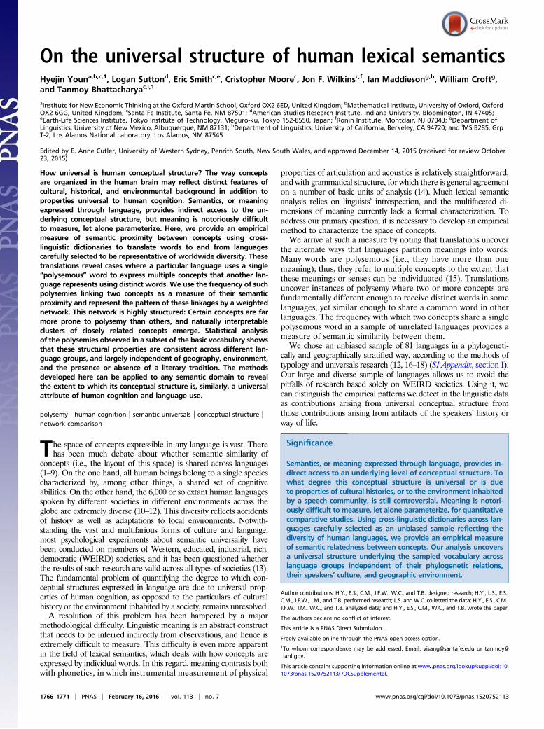
Constructing Semantic Network from TranslationsWe represent semantic relations obtained from dictionary transla-tions of the chosen concepts as a network. Two meanings are linkedif they can be reached from one another by a translation into somelanguage and then back. The link is weighted by the number of suchpaths (of length 2), that is, the number of polysemous words thatrepresent both meanings (details are provided in Materials andMethods). Fig. 1 illustrates the construction with examples from twolanguages. Translating the word SUN into Lakhota results in wí andáηpawí. Although the latter picks up no other meaning, wí is poly-semous: it possesses additional meanings of MOON and month, sothey are linked to SUN in the network. A similar polysemy is ob-served in Coast Tsimshian, where gyemk, the translation of SUN,
also means heat, thus providing a link between SUN and heat. Wewrite the initial Swadesh concepts (SUN and MOON in this ex-ample) in capital letters, whereas other concepts that arise throughtranslations (month and heat here) are written in lowercase letters.We restrict our study to the neighborhood of the initial Swadeshconcepts, so further translations of these latter concepts are notfollowed.With this approach, we can construct a semantic network for each
individual language. It is conceivable, however, that a group of lan-guages bears structural resemblances as a result of the speakers’sharing common historical or environmental features. A link betweenSUN and MOON, for example, recurs in both languages illustratedin Fig. 1, yet does not appear in many other languages, where otherlinks are seen instead. Thus, for example, SUN is linked to divinityand time in Japanese and to thirst and DAY/DAYTIME in theKhoisan language !Xóõ. The question is then the degree to whichthese semantic networks are similar across language groups, reflectinguniversal conceptual structure, and the extent to which they aresensitive to cultural or environmental variables, such as phylogenetichistory, climate, geography, or the presence of a literary tradition. Wetest such questions by constructing aggregate networks from groups oflanguages that share a common cultural and environmental propertyand comparing these networks between different language groups.
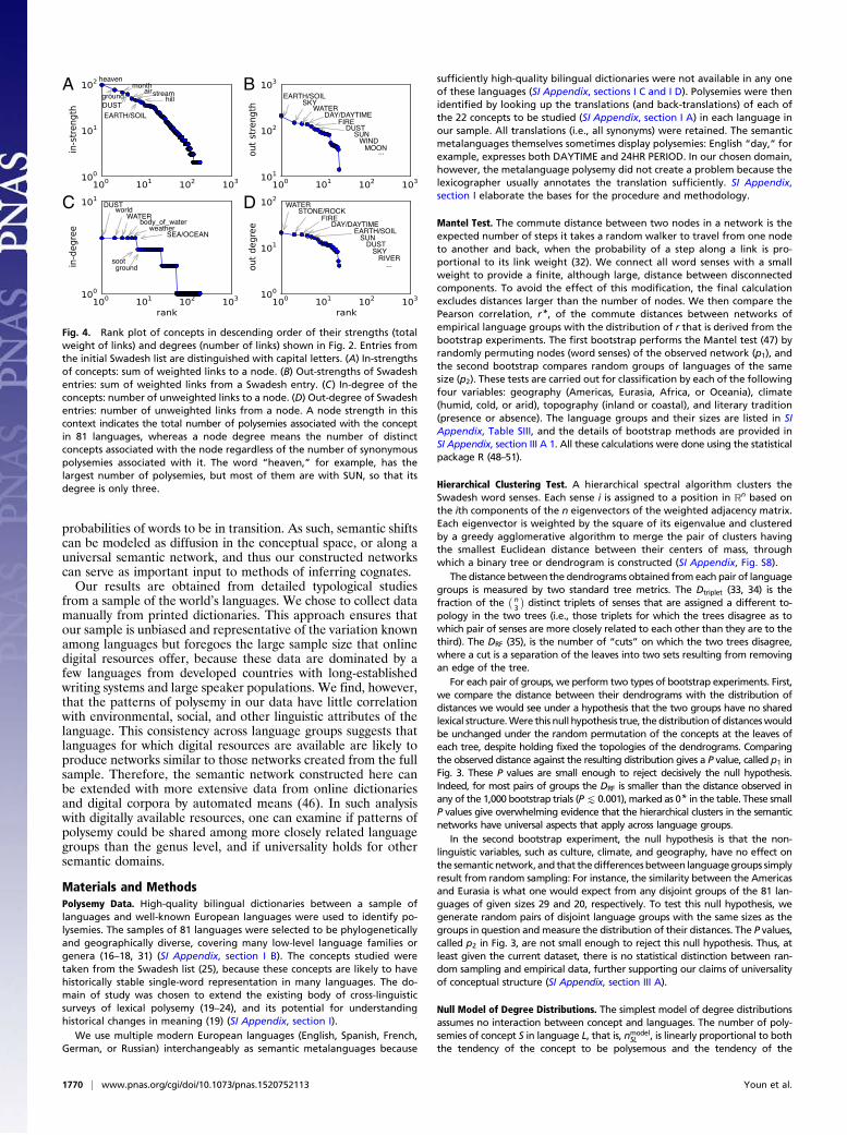
Semantic ClusteringsAs a point of comparison for the networks obtained from suchgroups of languages, we show the network obtained from the entireset of languages in Fig. 2 and SI Appendix, Fig. S6, displaying onlythe links that appear more than once. This network exhibits thebroad topological structure of polysemies observed in our data. Itreveals three almost disconnected clusters of concepts that are farmore prone to polysemy within each cluster than between them.These clusters admit a natural semantic interpretation. Thus, forexample, the semantically most uniform cluster, colored in blue,includes concepts related to water. A second, smaller cluster, col-ored in yellow, groups concepts related to solid natural materials(e.g., STONE/ROCK, MOUNTAIN) and associated landscapefeatures (e.g., forest, clearing, highlands). The third cluster, coloredin red, is more diverse, containing terrestrial terms (e.g., field, floor,ground, EARTH/SOIL), celestial objects [e.g., CLOUD(S), SKY,SUN, MOON], and units of time (e.g., DAY, NIGHT, YEAR).Although the clustering is strong, there do exist rare polysemiesthat occur only once in our dataset (and are thus not displayed inFig. 2) connecting the three clusters. Thus, for example, CLOUD(S)is polysemous with lightning in Albanian, whereas the latter ispolysemous with STONE/ROCK in !Xóõ, and whereas holy placeis a polysemy for MOUNTAIN in Kisi, it is instead polysemouswith LAKE in Wintu. The individual networks including suchweak links can be accessed in our web-based platform (29).The links defining each of the three clusters can be understood
in terms of well-known kinds of polysemies: metonymies (polysemybetween part and whole) and commonly found semantic extensionto hypernyms (more general concepts), hyponyms (more specificconcepts), and cohyponyms (specific concepts belonging to thesame category). The first cluster contains both liquid substancesand topographic features metonymically related to water. Thesubstance polysemies in this cluster are various liquids, cohypo-nyms of WATER. The topographic polysemies (e.g., LAKE,RIVER) are also linked as cohyponyms under “body of water” and“flowing water.” Similarly, in the third cluster, the bridge betweenthe terrestrial and celestial components is provided by the hypo-nyms of “granular aggregates,” which span both the terrestrialEARTH/SOIL, DUST, and SAND and the airborne SMOKEand CLOUD(S).
Evidence for Universal Semantic StructureThe semantic network across languages reveals a universal set ofrelationships among these concepts that possibly reflects human
gooypah gimgmdziws
MOON SUNheatmonth
Sample level: S
Words leveltranslation
Red: Coast_TsimshianBlue: Lakhota
Meaning level: m
ha
ha
SUN
gyemk
backtranslation
m
MOON
month heatMOON SUN
MOON SUN
6 4122 1
2
2 heatMOON
SUN
month2
2
2
1
1
A
B C
2
Unipartite: {m}
Fig. 1. Schematic figure of the construction of semantic networks. (A) Bipartitesemantic network constructed through translation (links from the first layer to thesecond layer) and back-translation (links from the second layer to the third layer)for the cases of MOON and SUN in two American languages: Coast Tsimshian (redlinks) and Lakhota (blue links). We write the starting concepts from the Swadeshlist (SUN, MOON) in capital letters, whereas other concepts that arise throughtranslation (month, heat) are in written in lowercase letters. (B) We link each pairof concepts with a weight equal to the number of translation–back-translationpaths. (C) Resulting weighted graph. More methodological information can befound in SI Appendix, section II.
Youn et al. PNAS | February 16, 2016 | vol. 113 | no. 7 | 1767
ANTH
ROPO
LOGY
PSYC
HOLO
GICALAND
COGNITIVESC
IENCE
S

conceptualization of these semantic domains (8, 12, 30). Alterna-tively, it has been postulated that such semantic relations arestrongly influenced by the physical environment that human soci-eties inhabit (31).To address this question, we group the languages by various
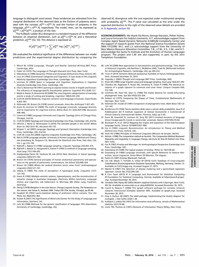
factors (SI Appendix, Table SIII) comprising the geography, cli-mate, or topography of the region where they are spoken, andthe presence or absence of a literary tradition in them, and wetest the effect of these factors on the semantic network. Wemeasured the similarity between these groups’ semantic networksin several ways. First, we measured the correlation between thecommute distances (32) between nearby concepts (Materials andMethods and SI Appendix, section III A 1). Then, to compare thesenetworks’ large-scale structure, we clustered the concepts in eachnetwork hierarchically as a dendrogram (SI Appendix, Fig. S8) andcompared them using two standard tree metrics (33–35): thetriplet distance (Dtriplet) and the Robinson–Foulds distance (DRF)(Materials and Methods and SI Appendix, section III A). To testwhether these networks are more similar than what we wouldexpect by chance, we performed bootstrap experiments, where wecompared each network with the one where the concepts wererandomly permuted (SI Appendix, section III). As shown by the p1values in Fig. 3, in every case, the networks of real language groupsare far more similar to each other than to these randomly per-muted networks, allowing us to reject decisively the null hypoth-esis that these semantic networks are completely uncorrelated(statistical details are provided in SI Appendix, section III B).
All these tests thus establish that different language groups doindeed have semantic structure in common. To explore this universalsemantic structure further, we tested a null hypothesis at the otherextreme, that cultural and environmental variables have no effect onthe semantic network. For this purpose, we performed a differentkind of bootstrap experiment, where we replaced each languagegroup with a random sample of the same size from the set of lan-guages. As denoted by p2 in Fig. 3, we find that, with rare exceptions,there is no statistical support (SI Appendix, section III B) for thehypothesis that the differences between the language groups studiedare any larger than between random groups of the same size. Thisfact means that the impacts of cultural and environmental factors areweaker than what can be established with our dataset; thus, ourresults are consistent with the hypothesis that semantic clusteringstructure is independent of culture and environment in thesesemantic domains.
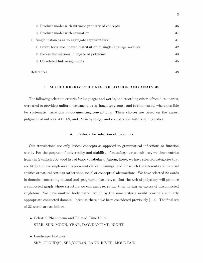
Heterogeneity of the Semantic NetworkThe universal semantic network shown in Fig. 2 is heterogeneousin both node degrees and link weights. The numbers of polysemiesinvolving individual meanings are uneven, possibly trending to-ward a heavy-tailed distribution (Fig. 4). This distribution indicatesthat concepts have different tendencies of being polysemous. Forexample, EARTH/SOIL has more than 100 polysemies, whereasSALT has only a few.Interestingly, we find that this heterogeneity is also universal: The
numbers of polysemies of the various concepts that we studied inany two languages are strongly correlated with each other. This
DUST
sawdust
soot
cloud_of_dust
pollen
dust_storm
cigarette
alcoholbeverage
SALT
juice
moisture
tide
WATERtemper_(of_metal)
interest_on_money
charmflavor
gunfire
flameblaze
burning_object
electricity
conflagrationfever
mold
ASH(ES)
embers
claypowder
country
gravel
mud
gunpowder
burned_object
SEA/OCEAN
stream
springcoast
RIVER
liquid
wave
EARTH/SOILfloor
bottom
debris
hole
ground
f i l th
field
homeland
flood
watercourse
flowing_water
torrent currentheat
firewoodpassion FIRE
angerhearth
moneyf l int
lump
gem
pebble
hailweight
battery
season
long_period_of_time
Christmasbirthday
summer
time
Pleiadeswinter
YEAR
SKY
atmosphere
abovehigh
top
air
space
chambered_nautilusmenseslunar_month
moonlight
menstruation_period
satelliteMOON
divinity
date
sunlight
weather
heat_of_sunSUN
month cold
mood
breeze
bodily_gases
breath
WIND
climate
direction
storm
STONE/ROCKcalculus
boulder
seedgallstone
cobble
MOUNTAIN
kidneystone
cliff
hi l l
metal
milestone pile
clearing
tombstoneforest
height24hr_period
heaven
ceiling
noon
thirst
swamp
pondwaterhole
tank
puddle
LAKEdawnafternoon
clock
DAY/DAYTIME
life
body_of_waterrain
sapbodily_fluid
lagoon
soup
teacolor
worldsandbank
NIGHT
evening beach
darknesslast_night
sandy_area
sleep
SAND
age
planet
celebrity asterisk
STAR
lodestarluck
fate
starfishheavenly_body
l ight
highlandsvolcano
slope
mountainous_region
mist
fog
haze
smell
CLOUD(S)
SMOKE fumes
tobacco
householdmatch
lampmeteor
burning clan
Fig. 2. Semantic network inferred from polysemy data. Concepts are linked when polysemous words cover both concepts. Swadesh words (the startingconcepts) are capitalized. The size of a node and the width of a link to another node are proportional to the number of polysemies associated with theconcept and with the two connected concepts, respectively. Links whose weights are at least 2 are shown, and their directions are omitted for simplicity. Thethick link from SKY to heaven, for example, shows that a large number of words in various languages have both SKY and heaven as meanings. Three distinctclusters, colored in red, blue, and yellow, are identified. These clusters may indicate a set of relationships among concepts that reflects a universal humanconceptual structure in these domains.
1768 | www.pnas.org/cgi/doi/10.1073/pnas.1520752113 Youn et al.

correlation holds despite the observation that the languages differ inthe overall magnitude of polysemy, so that the same concepts are farmore polysemous in some languages than in others (SI Appendix, Fig.S2). In fact, a simple formula predicts the number of polysemies, nSL,involving sense S in language L rather well (SI Appendix, Fig. S9):
nmodelSL ≡ nS ×
nLN, [1]
where nS is the number of polysemies involving sense S in theaggregate network from all languages, N is the total number ofpolysemies in this aggregate network, and nL is the number ofpolysemies in the language L. This formula is exactly what we wouldexpect (Materials and Methods and SI Appendix, section II B)if each language randomly and independently draws a subsetof polysemies for each concept S from the universal aggregatenetwork, which we can identify as an underlying “universal seman-tic space” (SI Appendix, Fig. S5). The data for only three concepts,MOON, SUN, and ASHES, deviate from this linear pattern bymore than the expected sampling errors (p≈ 0.01) in that theydisplay an initial rapid increase in nSL with nL, followed by asaturation or slower increase at larger values of nL (SI Appendix,Fig. S10). These deviations can be accommodated using a slightlymore complicated model described in SI Appendix, section IV.
DiscussionWe propose a principled method to construct semantic networkslinking concepts via polysemous words identified by cross-linguisticdictionaries. Based on the method, we found overwhelming evidencethat the semantic networks for different groups share a large amountof structure in common across geographic and cultural differences.Indeed, our results are consistent with the hypothesis that culturaland environmental factors have little statistically significant effect onthe semantic network of the subset of basic concepts studied here.
To a large extent, the semantic network appears to be a humanuniversal: For instance, SEA/OCEAN and SALT are more closelyrelated to each other than either is to SUN, and this pattern is truefor both coastal and inland languages.These findings have broad implications. Universal structures
in lexical semantics such as we observe can greatly aid re-construction of human history using linguistic data (37, 38).Much progress has been made in reconstructing the phylogeniesof word forms from known cognates in various languages, thanksto the ability to measure phonetic similarity and our knowledgeof the processes of sound change. The relationship between se-mantic similarity and semantic shift, however, is still poorly un-derstood. The standard view in historical linguistics is that anymeaning can change to any other meaning (39, 40), and noconstraint is imposed on what meanings can be compared withdetect cognates (41). In contrast to this view, we find that at leastsome similarities occur in a heterogeneous and clustered fashion.Previous studies (9, 19–21, 23, 24, 42–45) have investigated the
presence or absence of universality in how languages structurethe lexicon in a few semantic domains dealing with personalitems like body parts, perceptual elements like color metaphors,and cultural items like kinship relations. In this work, we studyinstead the domain of celestial and landscape objects that onemay a priori expect to be strongly affected by the environment.We find, however, that the semantic networks on which thesenatural objects lie are universal. It is generally accepted amonghistorical linguists that language change is gradual: Over his-torical time, words gain meanings when their use is extended tosimilar meanings and lose meanings when another word is ex-tended to the first word’s meaning. If such transitional situationsare common among polysemies, then the meaning shifts in thisdomain are likely to be equally universal, and the observedweights on different links of the semantic network reflect the
0.2 0.3 0.4 0.5 0.6 0.7
0.05
0.10
0.15
0.20
0.25
0.30
Americas vs. Oceania, triplet distanceA
Dtriplet
distribution
B
Fig. 3. (A) Illustration of our bootstrap experiments. The Dtriplet between the dendrograms of the Americas and Oceania is 0.56 (indicated by the downwardarrow) (33, 34). This value sits at the very low end of the distribution of distances generated by randomly permuted networks (the red-shaded profile on theright), but it is well within the distribution that we obtain by resampling random groups from the set of languages (the blue-shaded profile on the left). Thisfact gives strong evidence that each pair of groups shares an underlying semantic network, and that the differences between them are no larger than wouldresult from random sampling (details are provided in Materials and Methods). Therefore, these two language groups are much more closely related than ifconcepts were permuted randomly, showing they share a common semantic structure, but they are roughly as related as any pair of language groups of thesesizes, suggesting that the geographic and cultural difference between them have little effect on their structure. (B) Comparing distance metrics, the Pearsoncorrelation (r) between commute distances (32) on the semantic networks of groups and the Dtriplet and DRF among the corresponding dendrograms (33–35),on two bootstrap experiments to obtain p1 (Mantel test or randomly permuted dendrograms) and p2 (surrogate groups). The p1 values for the formerbootstrap (p2 values for the latter) are the fraction of 1,000 bootstrap samples whose distances are smaller (larger) than the observed distance. In either case,0* denotes a value below 0.001 (i.e., no bootstrap sample satisfied the condition). The Mantel test used 999 replicates for Pearson correlations to calculate p1
values, and 99 bootstrap samples (or 999 when marked with †) were used for p2. Given that we make 11 independent comparisons for any quantity, aBonferroni-corrected (36) significance threshold of p1,2 = 0.005 is appropriate for a nominal test size of p=0.05 (more extensively discussed in SI Appendix,section III B).
Youn et al. PNAS | February 16, 2016 | vol. 113 | no. 7 | 1769
ANTH
ROPO
LOGY
PSYC
HOLO
GICALAND
COGNITIVESC
IENCE
S
probabilities of words to be in transition. As such, semantic shiftscan be modeled as diffusion in the conceptual space, or along auniversal semantic network, and thus our constructed networkscan serve as important input to methods of inferring cognates.Our results are obtained from detailed typological studies
from a sample of the world’s languages. We chose to collect datamanually from printed dictionaries. This approach ensures thatour sample is unbiased and representative of the variation knownamong languages but foregoes the large sample size that onlinedigital resources offer, because these data are dominated by afew languages from developed countries with long-establishedwriting systems and large speaker populations. We find, however,that the patterns of polysemy in our data have little correlationwith environmental, social, and other linguistic attributes of thelanguage. This consistency across language groups suggests thatlanguages for which digital resources are available are likely toproduce networks similar to those networks created from the fullsample. Therefore, the semantic network constructed here canbe extended with more extensive data from online dictionariesand digital corpora by automated means (46). In such analysiswith digitally available resources, one can examine if patterns ofpolysemy could be shared among more closely related languagegroups than the genus level, and if universality holds for othersemantic domains.
Materials and MethodsPolysemy Data. High-quality bilingual dictionaries between a sample oflanguages and well-known European languages were used to identify po-lysemies. The samples of 81 languages were selected to be phylogeneticallyand geographically diverse, covering many low-level language families orgenera (16–18, 31) (SI Appendix, section I B). The concepts studied weretaken from the Swadesh list (25), because these concepts are likely to havehistorically stable single-word representation in many languages. The do-main of study was chosen to extend the existing body of cross-linguisticsurveys of lexical polysemy (19–24), and its potential for understandinghistorical changes in meaning (19) (SI Appendix, section I).
We use multiple modern European languages (English, Spanish, French,German, or Russian) interchangeably as semantic metalanguages because
sufficiently high-quality bilingual dictionaries were not available in any oneof these languages (SI Appendix, sections I C and I D). Polysemies were thenidentified by looking up the translations (and back-translations) of each ofthe 22 concepts to be studied (SI Appendix, section I A) in each language inour sample. All translations (i.e., all synonyms) were retained. The semanticmetalanguages themselves sometimes display polysemies: English “day,” forexample, expresses both DAYTIME and 24HR PERIOD. In our chosen domain,however, the metalanguage polysemy did not create a problem because thelexicographer usually annotates the translation sufficiently. SI Appendix,section I elaborate the bases for the procedure and methodology.
Mantel Test. The commute distance between two nodes in a network is theexpected number of steps it takes a random walker to travel from one nodeto another and back, when the probability of a step along a link is pro-portional to its link weight (32). We connect all word senses with a smallweight to provide a finite, although large, distance between disconnectedcomponents. To avoid the effect of this modification, the final calculationexcludes distances larger than the number of nodes. We then compare thePearson correlation, r*, of the commute distances between networks ofempirical language groups with the distribution of r that is derived from thebootstrap experiments. The first bootstrap performs the Mantel test (47) byrandomly permuting nodes (word senses) of the observed network (p1), andthe second bootstrap compares random groups of languages of the samesize (p2). These tests are carried out for classification by each of the followingfour variables: geography (Americas, Eurasia, Africa, or Oceania), climate(humid, cold, or arid), topography (inland or coastal), and literary tradition(presence or absence). The language groups and their sizes are listed in SIAppendix, Table SIII, and the details of bootstrap methods are provided inSI Appendix, section III A 1. All these calculations were done using the statisticalpackage R (48–51).
Hierarchical Clustering Test. A hierarchical spectral algorithm clusters theSwadesh word senses. Each sense i is assigned to a position in Rn based onthe ith components of the n eigenvectors of the weighted adjacency matrix.Each eigenvector is weighted by the square of its eigenvalue and clusteredby a greedy agglomerative algorithm to merge the pair of clusters havingthe smallest Euclidean distance between their centers of mass, throughwhich a binary tree or dendrogram is constructed (SI Appendix, Fig. S8).
The distance between the dendrograms obtained from each pair of languagegroups is measured by two standard tree metrics. The Dtriplet (33, 34) is thefraction of the
� n3
�distinct triplets of senses that are assigned a different to-
pology in the two trees (i.e., those triplets for which the trees disagree as towhich pair of senses are more closely related to each other than they are to thethird). The DRF (35), is the number of “cuts” on which the two trees disagree,where a cut is a separation of the leaves into two sets resulting from removingan edge of the tree.
For each pair of groups, we perform two types of bootstrap experiments. First,we compare the distance between their dendrograms with the distribution ofdistances we would see under a hypothesis that the two groups have no sharedlexical structure.Were this null hypothesis true, the distributionof distanceswouldbe unchanged under the random permutation of the concepts at the leaves ofeach tree, despite holding fixed the topologies of the dendrograms. Comparingthe observed distance against the resulting distribution gives a P value, called p1 inFig. 3. These P values are small enough to reject decisively the null hypothesis.Indeed, for most pairs of groups the DRF is smaller than the distance observed inany of the 1,000 bootstrap trials (PK0.001), marked as 0* in the table. These smallP values give overwhelming evidence that the hierarchical clusters in the semanticnetworks have universal aspects that apply across language groups.
In the second bootstrap experiment, the null hypothesis is that the non-linguistic variables, such as culture, climate, and geography, have no effect onthe semantic network, and that thedifferencesbetween languagegroups simplyresult from random sampling: For instance, the similarity between the Americasand Eurasia is what one would expect from any disjoint groups of the 81 lan-guages of given sizes 29 and 20, respectively. To test this null hypothesis, wegenerate random pairs of disjoint language groups with the same sizes as thegroups in question andmeasure the distribution of their distances. The P values,called p2 in Fig. 3, are not small enough to reject this null hypothesis. Thus, atleast given the current dataset, there is no statistical distinction between ran-dom sampling and empirical data, further supporting our claims of universalityof conceptual structure (SI Appendix, section III A).
Null Model of Degree Distributions. The simplest model of degree distributionsassumes no interaction between concept and languages. The number of poly-semies of concept S in language L, that is, nmodel
SL , is linearly proportional to boththe tendency of the concept to be polysemous and the tendency of the
A B
C D
Fig. 4. Rank plot of concepts in descending order of their strengths (totalweight of links) and degrees (number of links) shown in Fig. 2. Entries fromthe initial Swadesh list are distinguished with capital letters. (A) In-strengthsof concepts: sum of weighted links to a node. (B) Out-strengths of Swadeshentries: sum of weighted links from a Swadesh entry. (C) In-degree of theconcepts: number of unweighted links to a node. (D) Out-degree of Swadeshentries: number of unweighted links from a node. A node strength in thiscontext indicates the total number of polysemies associated with the conceptin 81 languages, whereas a node degree means the number of distinctconcepts associated with the node regardless of the number of synonymouspolysemies associated with it. The word “heaven,” for example, has thelargest number of polysemies, but most of them are with SUN, so that itsdegree is only three.
1770 | www.pnas.org/cgi/doi/10.1073/pnas.1520752113 Youn et al.
language to distinguish word senses. These tendencies are estimated from themarginal distribution of the observed data as the fraction of polysemy associ-ated with the concept, pdata
S =ndataS =N, and the fraction of polysemy in the
language, pdataL =ndata
L =N, respectively. The model, then, can be expressed aspmodelSL =pdata
S pdataL , a product of the two.
The Kullback–Leibler (KL) divergence is a standard measure of the differencebetween an empirical distribution, such as pdata
SL ≡ndataSL =N, and a theoretical
prediction, pmodelSL (52, 53). This distance is expressed as:
D�pdataSL
��pmodelSL
�≡
XS, L
pdataSL log
�pdataSL
.pmodelSL
�.
We evaluated the statistical significance of the differences between our modelpredictions and the experimental degree distribution by comparing the
observed KL divergence with the one expected under multinomial samplingwith probability pmodel
SL . The P value was calculated as the area under theexpected distribution to the right of the observed value (details are providedin SI Appendix, section IV).
ACKNOWLEDGMENTS. We thank Ilia Peiros, George Starostin, Petter Holme,and Laura Fortunato for helpful comments. H.Y. acknowledges support fromComplex Agent Based Dynamic Networks (CABDyN) Complexity Center andthe support of research grants from the National Science Foundation (GrantSMA-1312294). W.C. and L.S. acknowledge support from the University ofNew Mexico Resource Allocation Committee. T.B., J.F.W., E.S., C.M., and H.Y.acknowledge the Santa Fe Institute and the Evolution of Human Languagesprogram. The project and C.M. are also supported, in part, by the JohnTempleton Foundation.
1. Whorf BL (1956) Language, Thought and Reality: Selected Writing (MIT Press,Cambridge, MA).
2. Fodor JA (1975) The Language of Thought (Harvard Univ Press, New York).3. Wierzbicka A (1996) Semantics: Primes and Universals (Oxford Univ Press, Oxford, UK).4. Lucy JA (1992) Grammatical Categories and Cognition: A Case Study of the Linguistic
Relativity Hypothesis (Cambridge Univ Press, Cambridge, UK).5. Levinson SC (2003) Space in Language and Cognition: Explorations in Cognitive
Diversity (Cambridge Univ Press, Cambridge, UK).6. Choi S, Bowerman M (1991) Learning to express motion events in English and Korean:
The influence of language-specific lexicalization patterns. Cognition 41(1-3):83–121.7. Majid A, Boster JS, BowermanM (2008) The cross-linguistic categorization of everyday
events: a study of cutting and breaking. Cognition 109(2):235–250.8. Croft W (2010) Relativity, linguistic variation and language universals. CogniTextes
4:303–307.9. Witkowski SR, Brown CH (1978) Lexical universals. Annu Rev Anthropol 7:427–451.10. Evans N, Levinson SC (2009) The myth of language universals: Language diversity
and its importance for cognitive science. Behav Brain Sci 32(5):429–448, discussion448–494.
11. Comrie B (1989) Language Universals and Linguistic Typology (Univ of Chicago Press,Chicago), 2nd Ed.
12. Croft W (2003) Typology and Universals (Cambridge Univ Press, Cambridge, UK), 2nd Ed.13. Henrich J, Heine SJ, Norenzayan A (2010) The weirdest people in the world? Behav
Brain Sci 33(2-3):61–83, discussion 83–135.14. Shopen T, ed (2007) Language Typology and Syntactic Description (Cambridge Univ
Press, Cambridge, UK), 2nd Ed.15. Croft W, Cruse DA (2004) Cognitive Linguistics (Cambridge Univ Press, Cambridge, UK).16. Bell A (1978) Language samples. Universals of Human Language, Method and Theory,
eds Greenberg JH, Ferguson CA, Moravcsik EA (Stanford Univ Press, Palo Alto, CA),Vol 1, pp 123–156.
17. Rijkhoff J, Bakker D (1998) Language sampling. Linguistic Typology 2(3):263–314.18. Rijkhoff J, Bakker D, Hengeveld K, Kahrel P (1993) A method of language sampling.
Stud Lang 17(1):169–203.19. Koptjevskaja-Tamm M, Vanhove M, eds (2012) New directions in lexical typology.
Linguistics 50(3):373–743.20. Brown CH (1976) General principles of human anatomical partonomy and specula-
tions on the growth of partonomic nomenclature. Am Ethnol 3(3):400–424.21. Brown CH (1983) Where do cardinal direction terms come from? Anthropological
Linguistics 25(2):121–161.22. Viberg Å (1983) The verbs of perception: A typological study. Linguistics 21(1):
123–162.23. Evans N (1992) Multiple semiotic systems, hyperpolysemy, and the reconstruction of
semantic change in Australian languages. Diachrony Within Synchrony: LanguageHistory and Cognition, eds Kellermann G, Morrissey MD (Peter Lang, Frankfurt,Germany).
24. Derrig S (1978)Metaphor in the color lexicon. Chicago Linguistic Society, The Parasession onthe Lexicon, eds Farkas D, Jacobsen WM, Todrys KW (The Society, Chicago), pp 85–96.
25. Swadesh M (1952) Lexico-statistical dating of prehistoric ethnic contacts. Proc AmPhilos Soc 96(4):452–463.
26. Kessler B (2001) The Significance of Word Lists (Center for the Study of Language andInformation, Stanford, CA).
27. Lohr M (1998) Methods for the genetic classification of languages. PhD dissertation(University of Cambridge, Cambridge, UK).
28. Lohr M (2000) New approaches to lexicostatistics and glottochronology. Time Depthin Historical Linguistics, eds Renfrew C, McMahon AMS, Trask RL (McDonald Institutefor Archaeological Research, Cambridge, UK), pp 209–222.
29. Youn H (2015) Semantic Network (polysemy) Available at hyoun.me/language/index.html. Accessed December 22, 2015.
30. Vygotsky L (2002) Thought and Language (MIT Press, Cambridge, MA).31. Dryer MS (1989) Large linguistic areas and language sampling. Stud Lang 13(2):257–292.32. Chandra AK, Raghavan P, Ruzzo WL, Smolensy R, Tiwari P (1996) The electrical re-
sistance of a graph captures its commute and cover times. Comput Complex 6(4):312–340.
33. Critchlow DE, Pearl DK, Qian CL (1996) The triples distance for rooted bifurcatingphylogenetic trees. Syst Biol 45(3):323–334.
34. Dobson AJ (1975) Comparing the Shapes of Trees, Combinatorial Mathematics III(Springer, New York).
35. Robinson DF, Foulds LR (1981) Comparison of phylogenetic trees. Math Biosci 53(1-2):131–147.
36. Bonferroni CE (1936) Teoria statistica delle classi e calcolo delle probabilità. Issue 8 ofPubblicazioni del R Instituto Superiore di Scienze Economiche e Commerciali diFirenze (Libreria internazionale Seeber, Florence, Italy), pp 3–62.
37. Dunn M, Greenhill SJ, Levinson SC, Gray RD (2011) Evolved structure of languageshows lineage-specific trends in word-order universals. Nature 473(7345):79–82.
38. Bouckaert R, et al. (2012) Mapping the origins and expansion of the Indo-Europeanlanguage family. Science 337(6097):957–960.
39. Fox A (1995) Linguistic Reconstruction: An Introduction to Theory and Method(Oxford Univ Press, Oxford, UK).
40. Hock HH (1986) Principles of Historical Linguistics (Mouton de Gruyter, Berlin).41. Nichols J (1996) The comparative method as heuristic. The Comparative Method Reviewed:
Regularity and Irregularity in Language Change, eds Durie M, Ross M (Oxford Univ Press,New York).
42. Fox R (1967) Kinship and Marriage: An Anthropological Perspective (Cambridge UnivPress, Cambridge, UK).
43. Greenberg JH (1949) The logical analysis of kinship. Philos Sci 16(1):58–64.44. Greenberg JH (1966) Language Universals, with Special Reference to Feature Hier-
archies, Janua Linguarum, Series Minor 59 (Mouton, The Hague).45. Parkin R (1997) Kinship (Blackwell, Oxford).46. List J-M, Mayer T, Terhalle A, Urban M (2014) CLICS: Database of Cross-Linguistic
Colexifications (Forschungszentrum Deutscher Sprachatlas, Marburg, Germany), Version 1.0.Available at CLICS.lingpy.org. Accessed August 27, 2015.
47. Mantel N (1967) The detection of disease clustering and a generalized regressionapproach. Cancer Res 27(2):209–220.
48. R Core Team (2015) R: A Language and Environment for Statistical Computing(R Foundation for Statistical Computing, Vienna), Available at https://www.R-project.org/. Accessed November 30, 2015.
49. Venables WN, Ripley BD (2002)Modern Applied Statistics with S (Springer, New York),4th Ed. Available at www.stats.ox.ac.uk/pub/MASS4. Accessed November 30, 2015.
50. Csardi G, Nepusz T (2006) The igraph software package for complex networkresearch, InterJournal (Complex Systems) 1695. Available at igraph.org/. AccessedNovember 30, 2015.
51. Dray S, Dufour AB (2007) The ade4 package: Implementing the duality diagram forecologists. J Stat Softw 22(4):1–20.
52. Kullback S, Leibler RA (1951) On information and sufficiency. Annals of MathematicalStatistics 22(1):79–86.
53. Cover TM, Thomas JA (1991) Elements of Information Theory (Wiley, New York).
Youn et al. PNAS | February 16, 2016 | vol. 113 | no. 7 | 1771
ANTH
ROPO
LOGY
PSYC
HOLO
GICALAND
COGNITIVESC
IENCE
S

Supporting Information: On the Universal Structure of Human Lexical
Semantics
Hyejin Youn,1, 2, 3 Logan Sutton,4 Eric Smith,3, 5 Cristopher Moore,3 Jon F.
Wilkins,3, 6 Ian Maddieson,7, 8 William Croft,7 and Tanmoy Bhattacharya3, 9
1Institute for New Economic Thinking at the Oxford Martin School, Oxford, OX2 6ED, UK
2Mathematical Institute, University of Oxford, Oxford, OX2 6GG, UK
3Santa Fe Institute, 1399 Hyde Park Road, Santa Fe, NM 87501, USA
4American Studies Research Institute, Indiana University, Bloomington, IN 47405, USA
5Earth-Life Sciences Institute, Tokyo Institute of Technology,
2-12-1-IE-1 Ookayama, Meguro-ku, Tokyo, 152-8550, Japan
6Ronin Institute, Montclair, NJ 07043
7Department of Linguistics, University of New Mexico, Albuquerque, NM 87131, USA
8Department of Linguistics, University of California, Berkeley, CA 94720, USA
9MS B285, Grp T-2, Los Alamos National Laboratory, Los Alamos, NM 87545, USA.

2
CONTENTS
I. Methodology for Data Collection and Analysis 3
A. Criteria for selection of meanings 3
B. Criteria for selection of languages 4
C. Semantic analysis of word senses 6
D. Bidirectional translation, and linguists’ judgments on aggregation of meanings 9
E. Trimming, collapsing, projecting 15
II. Notation and Methods of Network Representation 16
A. Network representations 16
1. Multi-layer network representation 17
2. Directed-hyper-graph representation 19
3. Projection to directed simple graphs and aggregation over target languages 19
B. Model for semantic space represented as a topology 20
1. Interpretation of the model into network representation 21
2. Beyond the available sample data 22
C. The aggregated network of meanings 23
D. Synonymous polysemy: correlations within and among languages 23
E. Node degree and link presence/absence data 26
F. Node degree and Swadesh meanings 26
III. Universal Structure: Conditional dependence 27
A. Comparing semantic networks between language groups 28
1. Mantel test 28
2. Hierarchical clustering test 29
B. Statistical significance 32
C. Single-language graph size is a significant summary statistic 32
D. Conclusion 33
IV. Model for Degree of Polysemy 33
A. Aggregation of language samples 33
B. Independent sampling from the aggregate graph 34
1. Statistical tests 34
3
2. Product model with intrinsic property of concepts 36
3. Product model with saturation 37
C. Single instances as to aggregate representation 41
1. Power tests and uneven distribution of single-language p-values 42
2. Excess fluctuations in degree of polysemy 43
3. Correlated link assignments 45
References 48
I. METHODOLOGY FOR DATA COLLECTION AND ANALYSIS
The following selection criteria for languages and words, and recording criteria from dictionaries,
were used to provide a uniform treatment across language groups, and to compensate where possible
for systematic variations in documenting conventions. These choices are based on the expert
judgment of authors WC, LS, and IM in typology and comparative historical linguistics.
A. Criteria for selection of meanings
Our translations use only lexical concepts as opposed to grammatical inflections or function
words. For the purpose of universality and stability of meanings across cultures, we chose entries
from the Swadesh 200-word list of basic vocabulary. Among these, we have selected categories that
are likely to have single-word representation for meanings, and for which the referents are material
entities or natural settings rather than social or conceptual abstractions. We have selected 22 words
in domains concerning natural and geographic features, so that the web of polysemy will produce
a connected graph whose structure we can analyze, rather than having an excess of disconnected
singletons. We have omitted body parts—which by the same criteria would provide a similarly
appropriate connected domain—because these have been considered previously [1–4]. The final set
of 22 words are as follows:
• Celestial Phenomena and Related Time Units:
STAR, SUN, MOON, YEAR, DAY/DAYTIME, NIGHT
• Landscape Features:
SKY, CLOUD(S), SEA/OCEAN, LAKE, RIVER, MOUNTAIN
4
• Natural Substances:
STONE/ROCK, EARTH/SOIL, SAND, ASH(ES), SALT, SMOKE, DUST, FIRE, WATER,
WIND
B. Criteria for selection of languages
The statistical analysis of typological features of languages inevitably requires assumptions
about which observations are independent samples from an underlying generative process. Since
languages of the world have varying degrees of relatedness, language features are subject to Gal-
ton’s problem of non-independence of samples, which can only be overcome with a full historical
reconstruction of relations. However, long-range historical relations are not known or not accepted
for most language families of the world [5]. It has become accepted practice to restrict to single
representatives of each genus in statistical typological analyses [6, 7].1
In order to minimize redundant samples within our data, we selected only one language from
each genus-level family [8]. The sample consists of 81 languages chosen from 535 genera in order to
maximize geographical diversity, taking into consideration population size, presence or absence of a
written language, environment and climate, and availability of a good quality bilingual dictionary.
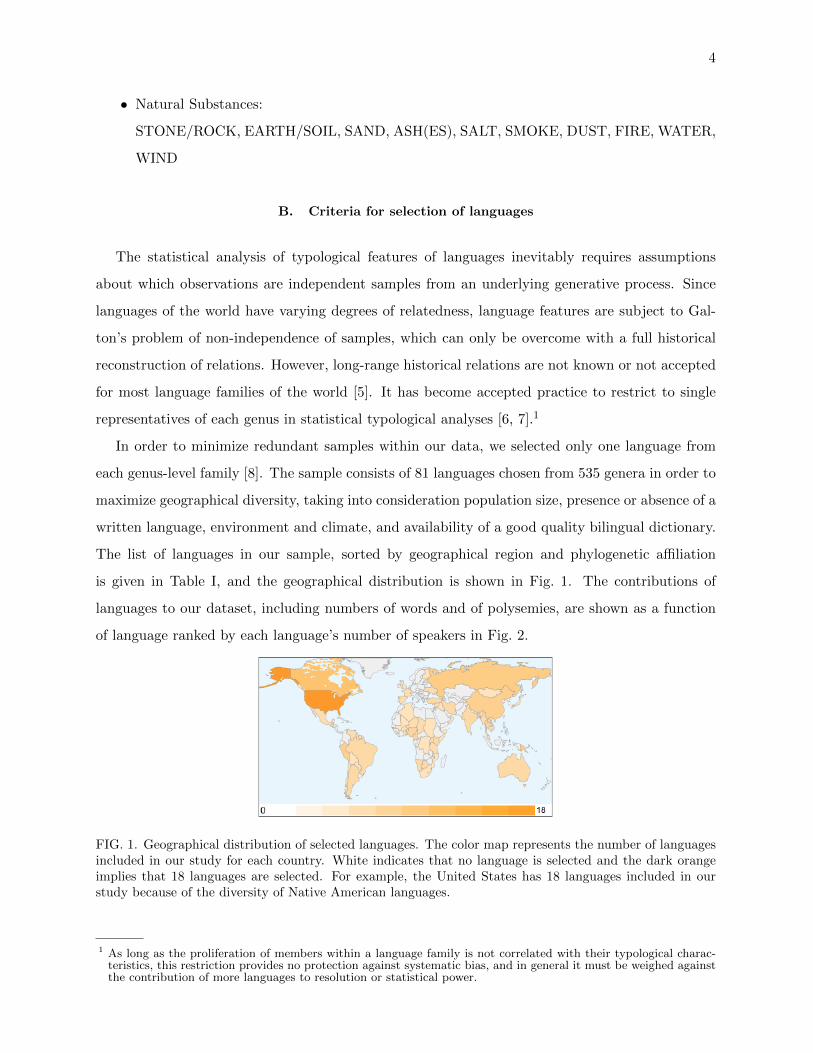
The list of languages in our sample, sorted by geographical region and phylogenetic affiliation
is given in Table I, and the geographical distribution is shown in Fig. 1. The contributions of
languages to our dataset, including numbers of words and of polysemies, are shown as a function
of language ranked by each language’s number of speakers in Fig. 2.
FIG. 1. Geographical distribution of selected languages. The color map represents the number of languagesincluded in our study for each country. White indicates that no language is selected and the dark orangeimplies that 18 languages are selected. For example, the United States has 18 languages included in ourstudy because of the diversity of Native American languages.
1 As long as the proliferation of members within a language family is not correlated with their typological charac-teristics, this restriction provides no protection against systematic bias, and in general it must be weighed againstthe contribution of more languages to resolution or statistical power.
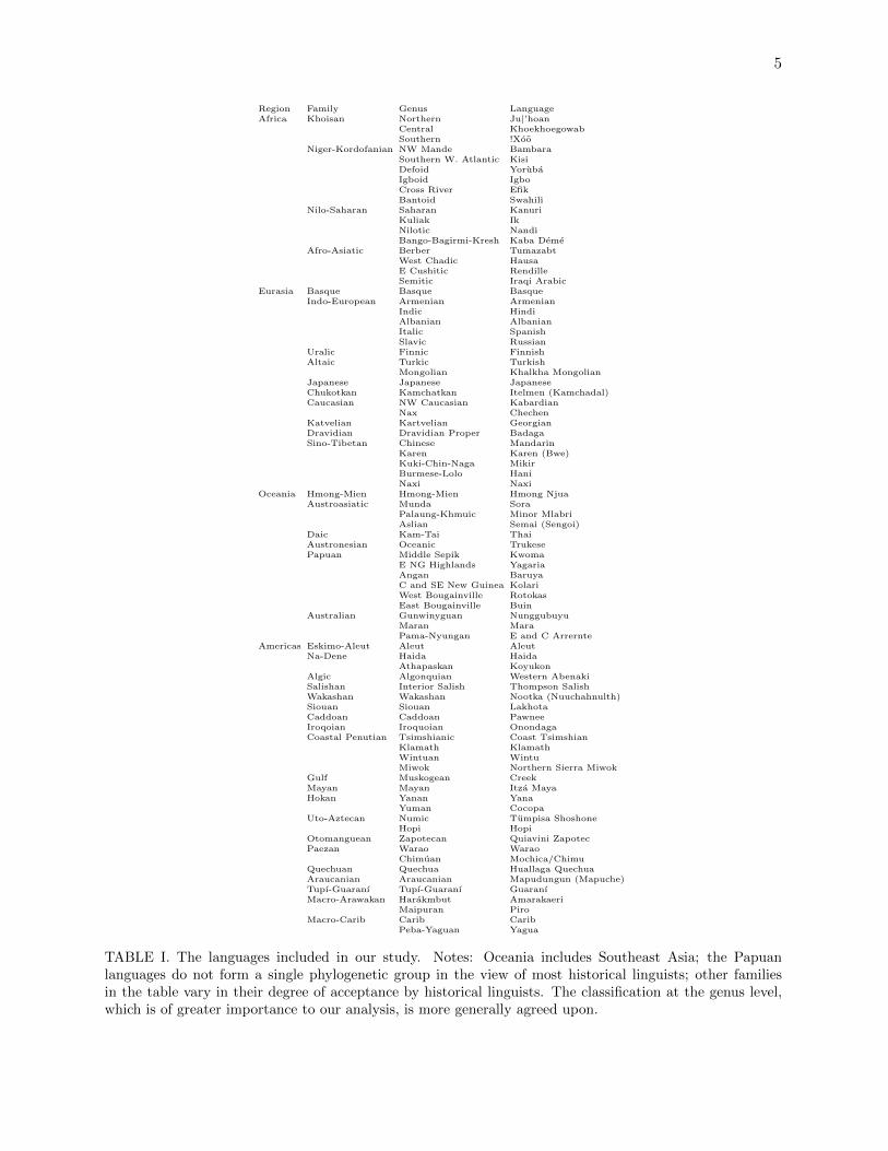
5
Region Family Genus LanguageAfrica Khoisan Northern Ju|’hoan
Central KhoekhoegowabSouthern !Xoo
Niger-Kordofanian NW Mande BambaraSouthern W. Atlantic KisiDefoid YorubaIgboid IgboCross River EfikBantoid Swahili
Nilo-Saharan Saharan KanuriKuliak IkNilotic NandiBango-Bagirmi-Kresh Kaba Deme
Afro-Asiatic Berber TumazabtWest Chadic HausaE Cushitic RendilleSemitic Iraqi Arabic
Eurasia Basque Basque BasqueIndo-European Armenian Armenian
Indic HindiAlbanian AlbanianItalic SpanishSlavic Russian
Uralic Finnic FinnishAltaic Turkic Turkish
Mongolian Khalkha MongolianJapanese Japanese JapaneseChukotkan Kamchatkan Itelmen (Kamchadal)Caucasian NW Caucasian Kabardian
Nax ChechenKatvelian Kartvelian GeorgianDravidian Dravidian Proper BadagaSino-Tibetan Chinese Mandarin
Karen Karen (Bwe)Kuki-Chin-Naga MikirBurmese-Lolo HaniNaxi Naxi
Oceania Hmong-Mien Hmong-Mien Hmong NjuaAustroasiatic Munda Sora
Palaung-Khmuic Minor MlabriAslian Semai (Sengoi)
Daic Kam-Tai ThaiAustronesian Oceanic TrukesePapuan Middle Sepik Kwoma
E NG Highlands YagariaAngan BaruyaC and SE New Guinea KolariWest Bougainville RotokasEast Bougainville Buin
Australian Gunwinyguan NunggubuyuMaran MaraPama-Nyungan E and C Arrernte
Americas Eskimo-Aleut Aleut AleutNa-Dene Haida Haida
Athapaskan KoyukonAlgic Algonquian Western AbenakiSalishan Interior Salish Thompson SalishWakashan Wakashan Nootka (Nuuchahnulth)Siouan Siouan LakhotaCaddoan Caddoan PawneeIroqoian Iroquoian OnondagaCoastal Penutian Tsimshianic Coast Tsimshian
Klamath KlamathWintuan WintuMiwok Northern Sierra Miwok
Gulf Muskogean CreekMayan Mayan Itza MayaHokan Yanan Yana
Yuman CocopaUto-Aztecan Numic Tumpisa Shoshone
Hopi HopiOtomanguean Zapotecan Quiavini ZapotecPaezan Warao Warao
Chimuan Mochica/ChimuQuechuan Quechua Huallaga QuechuaAraucanian Araucanian Mapudungun (Mapuche)Tupı-Guaranı Tupı-Guaranı GuaranıMacro-Arawakan Harakmbut Amarakaeri
Maipuran PiroMacro-Carib Carib Carib
Peba-Yaguan Yagua
TABLE I. The languages included in our study. Notes: Oceania includes Southeast Asia; the Papuanlanguages do not form a single phylogenetic group in the view of most historical linguists; other familiesin the table vary in their degree of acceptance by historical linguists. The classification at the genus level,which is of greater importance to our analysis, is more generally agreed upon.

6
FIG. 2. Vocabulary measures of languages in the dataset ranked in descending order of the size of the speakerpopulations. Population sizes are taken from Ethnologue. Each language is characterized by the numberof meanings in our polysemy dataset, of unique meanings, of non-unique meanings defined by exclusion ofall single occurrences, and of polysemous words (those having multiple meanings), plotted in blue, green,red, and cyan, respectively. We find a nontrivial correlation between population of speakers and data sizeof languages.
C. Semantic analysis of word senses
All of the bilingual dictionaries translated object language words into English, or in some
cases, Spanish, French, German or Russian (bilingual dictionaries in the other major languages
were used in order to gain maximal phylogenetic and geographic distribution). That is, we use
English and the other major languages as the semantic metalanguage for the word senses of the
object language words used in the analysis. English (or any natural language) is an imperfect
semantic metalanguage, because English itself has many polysemous words and divides the space
of concepts in a partly idiosyncratic way. This is already apparent in Swadesh’s own list: he
treated STONE/ROCK and EARTH/SOIL as synonyms, and had to specify that DAY referred
to DAYTIME as opposed to NIGHT, rather than a 24-hour period. However, the selection of a
concrete semantic domain including many discrete objects such as SUN and MOON allowed us to
avoid the much greater problems of semantic comparison in individuating properties and actions
or social and psychological concepts.
We followed lexicographic practice in individuating word senses across the languages. Lexicog-
raphers are aware of polysemies such as DAYTIME vs. 24 HOUR PERIOD and usually indicate
these semantic distinctions in their dictionary entries. There were a number of cases in which

7
different lexicographers appeared to use near-synonyms when the dictionaries were compared in
our cross-linguistic analysis. We believe that these choices of near-synonyms in English transla-
tions may not reflect genuine subtle semantic differences but may simply represent different choices
among near-synonyms made by different lexicographers. These near-synonyms were treated as a
single sense in the polysemy analysis; they are listed in Table II.
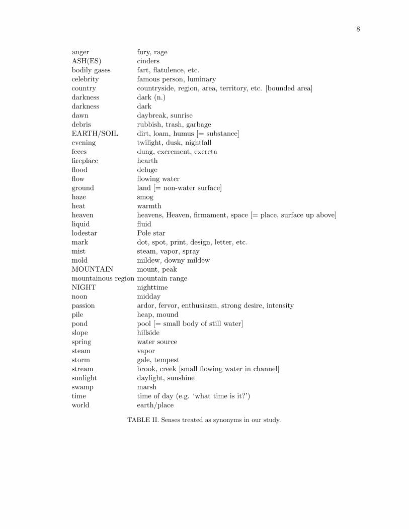
8
anger fury, rageASH(ES) cindersbodily gases fart, flatulence, etc.celebrity famous person, luminarycountry countryside, region, area, territory, etc. [bounded area]darkness dark (n.)darkness darkdawn daybreak, sunrisedebris rubbish, trash, garbageEARTH/SOIL dirt, loam, humus [= substance]evening twilight, dusk, nightfallfeces dung, excrement, excretafireplace hearthflood delugeflow flowing waterground land [= non-water surface]haze smogheat warmthheaven heavens, Heaven, firmament, space [= place, surface up above]liquid fluidlodestar Pole starmark dot, spot, print, design, letter, etc.mist steam, vapor, spraymold mildew, downy mildewMOUNTAIN mount, peakmountainous region mountain rangeNIGHT nighttimenoon middaypassion ardor, fervor, enthusiasm, strong desire, intensitypile heap, moundpond pool [= small body of still water]slope hillsidespring water sourcesteam vaporstorm gale, tempeststream brook, creek [small flowing water in channel]sunlight daylight, sunshineswamp marshtime time of day (e.g. ‘what time is it?’)world earth/place
TABLE II. Senses treated as synonyms in our study.

9
D. Bidirectional translation, and linguists’ judgments on aggregation of meanings
For each of the initial 22 Swadesh entries, we have recorded all translations from the met-
alanguage into the target languages, and then the back-translations of each of these into the
metalanguage. Back-translation results in the additional meanings beyond the original 22 Swadesh
meanings.
A word in a target language is considered polysemous if its back-translation includes multi-
ple words representing multiple senses as described in subsection I C. In cases where the back-
translation produces the same sense through more than one word in the target language, we call
it synonymous polysemy, and we take into account the degeneracy of each such polysemy in our
analysis as weighted links. The set of translations/back-translations of all 22 Swadesh meanings
for each target language constitutes our characterization of that language. The pool of translations
over the 81 target languages is the complete data set.
The dictionaries used in our study are listed below.
1. Dickens, Patrick. 1994. English-Ju|’hoan, Ju|’hoan-English dictionary. Koln: Rudiger
Koppe Verlag.
2. Haacke, Wilfrid H. G. and Eliphas Eiseb. 2002. A Khoekhoegowab dictionary, with an
English-Khoekhoegowab index. Windhoek: Gamsberg Macmillan.
3. Traill, Anthony. 1994. A !Xoo dictionary. Koln: Rudiger Koppe Verlag.
4. Bird, Charles and Mamadou Kante. Bambara-English English-Bambara Student Lexicon.
Bloomington: Indiana University Linguistics Club.
5. Childs, G. Tucker. 2000. A dictionary of the Kisi language, with an English-Kisi index.
Koln: Rudiger Koppe Verlag.
6. Wakeman, C. W. (ed.). 1937. A dictionary of the Yoruba language. Ibadan: Oxford Uni-
versity Press.
7. Abraham, R. C. 1958. Dictionary of modern Yoruba. London: University of London Press.
8. Welmers, Beatrice F. & William E. Welmers. 1968. Igbo: a learners dictionary. Los Angeles:
University of California, Los Angeles and the United States Peace Corps.
9. Goldie, Hugh. 1964. Dictionary of the Efik Language. Ridgewood, N.J.
10. Awde, Nicholas. 2000. Swahili Practical Dictionary. New York: Hippocrene Books.
11. Johnson, Frederick. 1969. Swahili-English Dictionary. New York: Saphrograph.
12. Kirkeby, Willy A. 2000. English-Swahili Dictionary. Dar es Salaam: Kakepela Publishing
Company (T) LTD.
10
13. Cyffer, Norbert. 1994. English-Kanuri Dictionary. Koln: Rudiger Koppe Verlag.
14. Cyffer, Norbert and John Hutchison (eds.). 1990. A Dictionary of the Kanuri Language.
Dordrecht: Foris Publications.
15. Heine, Bernd. 1999. Ik dictionary. Koln: Rudiger Koppe Verlag.
16. Creider, Jane Tapsubei and Chet A. Creider. 2001. A Dictionary of the Nandi Language.
Koln: Rudiger Koppe Verlag.
17. Palayer, Pierre, with Massa Solekaye. 2006. Dictionnaire deme (Tchad), precede de notes
grammaticales. Louvain: Peeters.
18. Delheure, J. 1984. Dictionnaire mozabite-francais. Paris: SELAF. [Tumzabt]
19. Abraham, R. C. 1962. Dictionary of the Hausa language (2nd ed.). London: University of
London Press.
20. Awde, Nicholas. 1996. Hausa-English English-Hausa Dictionary. New York: Hippocrene
Books.
21. Skinner, Neil. 1965. Kamus na turanci da hausa: English-Hausa Dictionary. Zaria, Nigeria:
The Northern Nigerian Publishing Company.
22. Pillinger, Steve and Letiwa Galboran. 1999. A Rendille Dictionary. Koln: Rudiger Koppe
Verlag.
23. Clarity, Beverly E., Karl Stowasser, and Ronald G. Wolfe (eds.) and D. R. Woodhead and
Wayne Beene (eds.). 2003. A dictionary of Iraqi Arabic: English-Arabic, Arabic-English.
Washington, DC: Georgetown University Press.
24. Aulestia, Gorka. 1989. Basque-English Dictionary. Reno: University of Nevada Press.
25. Aulestia, Gorka and Linda White. 1990. English-Basque Dictionary. Reno:University of
Nevada Press.
26. Aulestia, Gorka and Linda White. 1992. Basque-English English-Basque Dictionary. Reno:
University of Nevada Press.
27. Koushakdjian, Mardiros and Dicran Khantrouni. 1976. English-Armenian Modern Dictio-
nary. Beirut: G. Doniguian & Sons.
28. McGregor, R.S. (ed.). 1993. The Oxford Hindi-English Dictionary. Oxford: Oxford Univer-
sity Press.
29. Pathak, R.C. (ed.). 1966. Bhargavas Standard Illustrated Dictionary of the English Language
(Anglo-Hindi edition). Chowk, Varanasi, Banaras: Shree Ganga Pustakalaya.
30. Prasad, Dwarka. 2008. S. Chands Hindi-English-Hindi Dictionary. New Delhi: S. Chand &
Company.
11
31. Institut Nauk Narodnoj Respubliki Albanii. 1954. Russko-Albanskij Slovar’. Moscow: Go-
sudarstvennoe Izdatel’stvo Inostrannyx i Natsional’nyx Slovarej.
32. Newmark, Leonard (ed.). 1998. Albanian-English Dictionary. Oxford/New York: Oxford
University Press.
33. Orel, Vladimir. 1998. Albanian Etymological Dictionary. Leiden/Boston/Koln: Brill.
34. MacHale, Carlos F. et al. 1991. VOX New College Spanish and English Dictionary. Lincol-
nwood, IL: National Textbook Company.
35. The Oxford Spanish Dictionary. 1994. Oxford/New York/Madrid: Oxford University Press.
36. Mjuller, V. K. Anglo-russkij Slovar’. Izd. Sovetskaja Enciklopedija.
37. Ozhegov. Slovar’ Russkogo Jazyka. Gos. Izd. Slovarej.
38. Smirnickij, A. I. Russko-anglijskij Slovar’. Izd. Sovetskaja Enciklopedija.
39. Hurme, Raija, Riitta-Leena Malin, and Olli Syaoja. 1984. Uusi Suomi-Englanti Suur-
Sanakirja. Helsinki: Werner Soderstrom Osakeyhtio.
40. Hurme, Raija, Maritta Pesonen, and Olli Syvaoja. 1990. Englanti-Suomi Suur-Sanakirja:
English-Finnish General Dictionary. Helsinki: Werner Soderstrom Osakeyhtio.
41. Bayram, Ali, S. Serdar Turet, and Gordon Jones. 1996. Turkish-English Comprehensive
Dictionary. Istanbul: Fono/Hippocrene Books.
42. Hony, H. C. 1957. A Turkish-English Dictionary. Oxford: Oxford University Press.
43. Bawden, Charles. 1997. Mongolian-English Dictionary. London/New York: Kegan Paul
International.
44. Hangin, John G. 1970. A Concise English-Mongolian Dictionary. Indiana University Pub-
lications Volume 89, Uralic and Altaic Series. Bloomington: Indiana University.
45. Masuda, Koh (Ed.). 1974. Kenkyushas New Japanese-English Dictionary. Tokyo: Kenkyusha
Limited.
46. Worth, Dean S. 1969. Dictionary of Western Kamchadal. (University of California Publica-
tions in Linguistics 59.) Berkeley and Los Angeles: University of California Press.
47. Jaimoukha, Amjad M. 1997. Kabardian-English Dictionary, Being a Literary Lexicon of
East Circassian (First Edition). Amman: Sanjalay Press.
48. Klimov, G.A. and M.S. Xalilov. 2003. Slovar Kavkazskix Jazykov. Moscow: Izdatelskaja
Firma.
49. Lopatinskij, L. 1890. Russko-Kabardinskij Slovar i Kratkoju Grammatikoju. Tiflis: Ti-
pografija Kantseljarii Glavnonacalstvujuscago grazdanskoju castju na Kavkaz.
50. Aliroev, I. Ju. 2005. Cecensko-Russkij Slovar. Moskva: Akademia.
12
51. Aliroev, I. Ju. 2005. Russko-Cecenskij Slovar. Moskva: Akademia.
52. Amirejibi, Rusudan, Reuven Enoch, and Donald Rayfield. 2006. A Comprehensive Georgian-
English Dictionary. London: Garnett Press.
53. Gvarjalaze, Tamar. 1974. English-Georgian and Georgian-English Dictionary. Tbilisi:
Ganatleba Publishing House.
54. Hockings, Paul and Christiane Pilot-Raichoor. 1992. A Badaga-English dictionary. Berlin:
Mouton de Gruyter.
55. Institute of Far Eastern Languages, Yale University. 1966. Dictionary of Spoken Chinese.
New Haven: Yale University Press.
56. Henderson Eugenie J. A. 1997. Bwe Karen Dictionary, with texts and English-Karen word
list, vol. II: dictionary and word list. London: University of London School of Oriental and
African Studies.
57. Walker, G. D. 1925/1995. A dictionary of the Mikir language. New Delhi: Mittal Publica-
tions (reprint).
58. Lewis, Paul and Bai Bibo. 1996. Hani-English, English-Hani dictionary. London: Kegan
Paul International.
59. Pinson, Thomas M. 1998. Naqxi-Habaq-Yiyu Geezheeq Ceeqhuil: Naxi-Chinese-English Glos-
sary with English and Chinese index. Dallas: Summer Institute of Linguistics.
60. Heimbach, Ernest E. 1979. White Hmong-English Dictionary. Ithaca: Cornell Southeast
Asia Program, Linguistic Series IV.
61. Ramamurti, Rao Sahib G.V. 1933. English-Sora Dictionary. Madras: Government Press.
62. Ramamurti, Rao Sahib G.V. 1986. Sora-English Dictionary. Delhi: Mittal Publications.
63. Rischel, Jørgen. 1995. Minor Mlabri: a hunter-gatherer language of Northern Indochina.
Copenhagen: Museum Tusculanum Press.
64. Means, Nathalie and Paul B. Means. 1986. Sengoi-English, English-Sengoi dictionary.
Toronto: The Joint Centre on Modern East Asia, University of Toronto and York University.
[Semai]
65. Becker, Benjawan Poomsan. 2002. Thai-English, English-Thai Dictionary. Bangkok/Berkeley:
Paiboon Publishing.
66. Goodenough, Ward and Hiroshi Sugita. 1980. Trukese-English dictionary. (Memoirs of the
American Philosophical Society, 141.) Philadelphia: American Philosophical Society.
67. Goodenough, Ward and Hiroshi Sugita. 1990. Trukese-English dictionary, Supplementary
volume: English-Trukese and index of Trukese word roots. (Memoirs of the American Philo-
13
sophical Society, 141S.) Philadelphia: American Philosophical Society.
68. Bowden, Ross. 1997. A dictionary of Kwoma, a Papuan language of the north-east New
Guinea. (Pacific Linguistics, C-134.) Canberra: The Australian National University.
69. Renck, G. L. 1977. Yagaria dictionary. (Pacific Linguistics, Series C, No. 37.) Canberra:
Research School of Pacific Studies, Australian National University.
70. Lloyd, J. A. 1992. A Baruya-Tok Pisin-English dictionary. (Pacific Linguistics, C-82.)
Canberra: The Australian National University.
71. Dutton, Tom. 2003. A dictionary of Koiari, Papua New Guinea, with grammar notes.
(Pacific Linguistics, 534.) Canberra: Australia National University.
72. Firchow, Irwin, Jacqueline Firchow, and David Akoitai. 1973. Vocabulary of Rotokas-Pidgin-
English. Ukarumpa, Papua New Guinea: Summer Institute of Linguistics.
73. Laycock, Donald C. 2003. A dictionary of Buin, a language of Bougainville. (Pacific Lin-
guistics, 537.) Canberra: The Australian National University.
74. Heath, Jeffrey. 1982. Nunggubuyu Dictionary. Canberra: Australian Institute of Aboriginal
Studies.
75. Heath, Jeffrey. 1981. Basic Materials in Mara: Grammar, Texts, Dictionary. (Pacific Lin-
guistics, C60.) Canberra: Research School of Pacific Studies, Australian National University.
76. Henderson, John and Veronica Dobson. 1994. Eastern and Central Arrernte to English
Dictionary. Alice Springs: Institute for Aboriginal Development.
77. Bergsland, Knut. 1994. Aleut dictionary: unangam tunudgusii. Fairbanks: Alaska Native
Language Center, University of Alaska.
78. Enrico, John. 2005. Haida dictionary: Skidegate, Masset and Alaskan dialects, 2 vols. Fair-
banks and Juneau, Alaska: Alaska Native Language Center and Sealaska Heritage Institute.
79. Jette, Jules and Eliza Jones. 2000. Koyukon Athabaskan dictionary. Fairbanks: Alaska
Native Language Center.
80. Day, Gordon M. 1994. Western Abenaki Dictionary. Hull, Quebec: Canadian Museum of
Civilization.
81. Thompson, Laurence C. and M. Terry Thompson (compilers). 1996. Thompson River Sal-
ish Dictionary. (University of Montana Occasional Papers in Linguistics 12.). Missoula,
Montana: University of Montana Linguistics Laboratory.
82. Stonham, John. 2005. A Concise Dictionary of the Nuuchahnulth Language of Vancouver
Island. Native American Studies 17. Lewiston/Queenston/Lampeter: The Edwin Mellen
Press.

14
83. Lakota Language Consortium. 2008. New Lakota Dictionary. Bloomington: Lakhota Lan-
guage Consortium.
84. Parks, Douglas R. and Lula Nora Pratt. 2008. A dictionary of Skiri Pawnee. Lincoln:
University of Nebraska Press.
85. Woodbury, Hanni. 2003. Onondaga-English / English-Onondaga Dictionary. Toronto: Uni-
versity of Toronto Press.
86. Dunn, John Asher. Smalgyax: A Reference Dictionary and Grammar for the Coast
Tsimshian Language. Seattle: University of Washington Press. [Coast Tsimshian]
87. Barker, M. A. R. 1963. Klamath Dictionary. University of California Publications in Lin-
guistics 31. Berkeley: University of California Press.
88. Pitkin, Harvey. Wintu Dictionary. (University of California Publications in Linguistics, 95).
Berkeley and Los Angeles: University of California Press.
89. Callaghan, Catherine A. 1987. Northern Sierra Miwok Dictionary. University of California
Publications in Linguistics 110. Berkeley/Los Angeles/London: University of California
Press.
90. Martin, Jack B. and Margaret McKane Mauldin. 2000. A dictionary of Creek/Muskogee.
Omaha: University of Nebraska Press.
91. Hofling, Charles Andrew and Felix Fernando Tesucun. 1997. Itzaj Maya-Spanish-English
Dictionary/Diccionario Maya Itaj-Espanol-Ingles. Salt Lake City: University of Utah Press.
92. Sapir, Edward and Morris Swadesh. Yana Dictionary (University of California Papers in
Linguistics, 22). Berkeley: University of California Press.
93. Crawford, James Mack, Jr. 1989. Cocopa Dictionary. University of California Publications
in Linguistics Vol. 114, University of California Press.
94. Dayley, Jon P. 1989. Tumpisa (Panamint) Shoshone Dictionary. (University of California
Publications in Linguistics 116.) Berkeley: Univ. of California Press.
95. Hopi Dictionary Project (compilers). 1998. Hopi Dictionary/Hopıikwa Lavaytutuveni: A
Hopi-English dictionary of the Third Mesa Dialect. Tucson: University of Arizona Press.
96. Munro, Pamela, & Felipe H. Lopez. 1999. Di’csyonaary X:tee’n Dıi’zh Sah Sann Lu’uc: San
Lucas Quiavinı Zapotec Dictionary: Diccionario Zapoteco de San Lucas Quiavinı (2 vols.).
Los Angeles: UCLA Chicano Studies Research Center.
97. de Barral, Basilio M.a. 1957. Diccionario Guarao-Espanol, Espanol-Guarao. Sociedad de
Ciencias Naturales La Salle, Monografias 3. Caracas: Editorial Sucre.
98. Bruning, Hans Heinrich. 2004. Mochica Worterbuch/Diccionario Mochica: Mochica-

15
Castellano/Castellano-Mochica. Lima: Universidad de San Martin de Porres, Escuela
Profesional de Turismo y Hotelerıa.
99. Salas, Jose Antonio. 2002. Diccionario Mochica-Castellano/Castellano-Mochica. Lima:
Universidad de San Martin de Porres, Escuela Profesional de Turismo y Hotelerıa.
100. Weber, David John, Felix Cayco Zambrano, Teodoro Cayco Villar, Marlene Ballena Dvila.
1998. Rimaycuna: Quechua de Huanuco. Lima: Instituto Linguıstico de Verano.
101. Catrileo, Marıa. 1995. Diccionario Linguistico-Etnografico de la Lengua Mapuche. Santiago:
Editorial Andres Bello.
102. Erize, Esteban. 1960. Diccionario Comentado Mapuche-Espanol. Buenos Aires: Cuadernos
del Sur.
103. Britton, A. Scott. 2005. Guaranı-English, English-Guaranı Concise Dictionary. New York:
Hippocrene Books, Inc.
104. Mayans, Antonio Ortiz. 1973. Nuevo Diccionario Espanol-Guaranı, Guarani-Espanol
(Decima Edicion). Buenos Aires: Librerıa Platero Editorial.
105. Tripp, Robert. 1995. Diccionario Amarakaeri-Castellano. Serie Linguıstica Peruana 34.
Instituto Linguıstico de Verano: Ministerio de Educacion.
106. Matteson, Esther. 1965. The Piro (Arawakan) Language. University of California Publica-
tions in Linguistics 42. Berkeley/Los Angeles: University of California Press.
107. Mosonyi, Jorge C. 2002. Diccionario Basico del Idioma Karina. Barcelona, Venezuela:
Gobernacion del Estado Anzoategui, Direccion de Cultura, Fondo Editorial del Caribe.
108. Powlison, Paul S. 1995. Nijyami Niquejadamusiy May Niquejadamuju, May Niquejadamusiy
Nijyami Niquejadamuju: Diccionario Yagua-Castellano. Serie Linguıstica Peruana 35. In-
stituto Linguıstico de Verano: Ministerio de Educacion.
E. Trimming, collapsing, projecting
Our choice of starting categories is meant to minimize culturally or geographically specific
associations, but inevitably these enter through polysemy that results from metaphor or metonymy.
To attempt to identify polysemies that express some degree of cognitive universality rather than
pure cultural “accident”, we include in this report only polysemies that occurred in two or more
languages in the sample. The original data comprises 2263 words, translated from a starting list of
22 Swadesh meanings, and 826 meanings as distinguished by English translations. After removal
of the polysemies occurring in only a single language, the dataset was reduced to 2257 words and
16
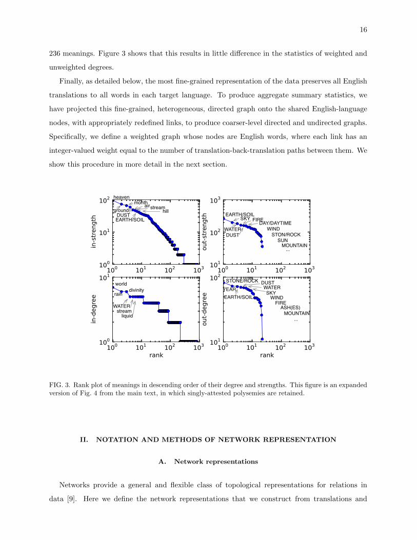
236 meanings. Figure 3 shows that this results in little difference in the statistics of weighted and
unweighted degrees.
Finally, as detailed below, the most fine-grained representation of the data preserves all English
translations to all words in each target language. To produce aggregate summary statistics, we
have projected this fine-grained, heterogeneous, directed graph onto the shared English-language
nodes, with appropriately redefined links, to produce coarser-level directed and undirected graphs.
Specifically, we define a weighted graph whose nodes are English words, where each link has an
integer-valued weight equal to the number of translation-back-translation paths between them. We
show this procedure in more detail in the next section.
heaven
groundmonth
DUST
airstream
EARTH/SOILhill EARTH/SOIL
SKY
WATER
FIRE
DUST
DAY/DAYTIME
world
raindivinity
WATERstreamliquid
STONE/ROCKYEAREARTH/SOIL
DUSTWATERSKYWINDFIREASH(ES)MOUNTAIN
...
WINDSTON/ROCKSUNMOUNTAIN...
FIG. 3. Rank plot of meanings in descending order of their degree and strengths. This figure is an expandedversion of Fig. 4 from the main text, in which singly-attested polysemies are retained.
II. NOTATION AND METHODS OF NETWORK REPRESENTATION
A. Network representations
Networks provide a general and flexible class of topological representations for relations in
data [9]. Here we define the network representations that we construct from translations and
17
back-translation to identify polysemies.
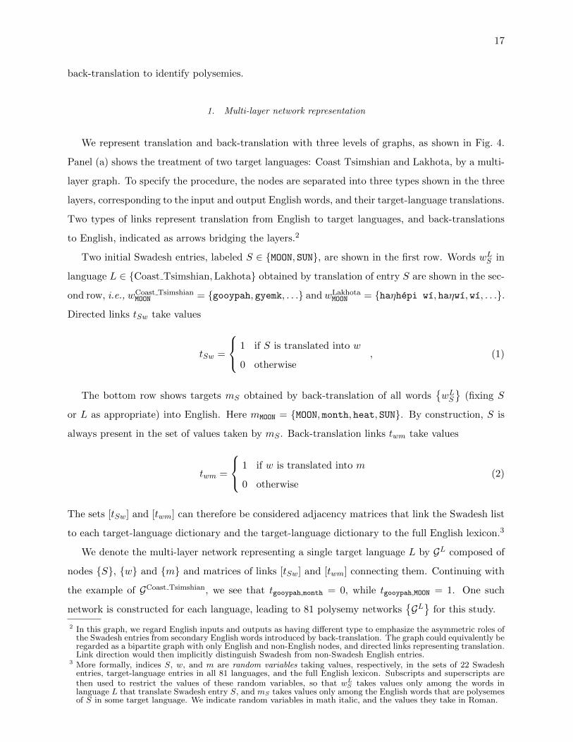
1. Multi-layer network representation
We represent translation and back-translation with three levels of graphs, as shown in Fig. 4.
Panel (a) shows the treatment of two target languages: Coast Tsimshian and Lakhota, by a multi-
layer graph. To specify the procedure, the nodes are separated into three types shown in the three
layers, corresponding to the input and output English words, and their target-language translations.
Two types of links represent translation from English to target languages, and back-translations
to English, indicated as arrows bridging the layers.2
Two initial Swadesh entries, labeled S ∈ {MOON, SUN}, are shown in the first row. Words wLS in
language L ∈ {Coast Tsimshian,Lakhota} obtained by translation of entry S are shown in the sec-
ond row, i.e., wCoast TsimshianMOON = {gooypah, gyemk, . . .} and wLakhota
MOON = {haηhepi wı, haηwı, wı, . . .}.
Directed links tSw take values
tSw =
1 if S is translated into w
0 otherwise, (1)
The bottom row shows targets mS obtained by back-translation of all words{wLS}
(fixing S
or L as appropriate) into English. Here mMOON = {MOON, month, heat, SUN}. By construction, S is
always present in the set of values taken by mS . Back-translation links twm take values
twm =
1 if w is translated into m
0 otherwise(2)
The sets [tSw] and [twm] can therefore be considered adjacency matrices that link the Swadesh list
to each target-language dictionary and the target-language dictionary to the full English lexicon.3
We denote the multi-layer network representing a single target language L by GL composed of
nodes {S}, {w} and {m} and matrices of links [tSw] and [twm] connecting them. Continuing with
the example of GCoast Tsimshian, we see that tgooypah,month = 0, while tgooypah,MOON = 1. One such
network is constructed for each language, leading to 81 polysemy networks{GL}
for this study.
2 In this graph, we regard English inputs and outputs as having different type to emphasize the asymmetric roles ofthe Swadesh entries from secondary English words introduced by back-translation. The graph could equivalently beregarded as a bipartite graph with only English and non-English nodes, and directed links representing translation.Link direction would then implicitly distinguish Swadesh from non-Swadesh English entries.
3 More formally, indices S, w, and m are random variables taking values, respectively, in the sets of 22 Swadeshentries, target-language entries in all 81 languages, and the full English lexicon. Subscripts and superscripts arethen used to restrict the values of these random variables, so that wLS takes values only among the words inlanguage L that translate Swadesh entry S, and mS takes values only among the English words that are polysemesof S in some target language. We indicate random variables in math italic, and the values they take in Roman.
18
...
gyemgmáatkgooypah gimgmdziws
MOON SUNheatmonth
Sample level: S
Words level: wLtranslation tSw
áŋpawí
Red: Coast_TsimshianBlue: Lakhota
wí
Meaning level: m
haŋhépi_wí
haŋwí
SUN
gyemk
backtranslation twm
m
wC wL
MOON
month heatMOON SUN
MOON SUN
6 4122 12
2
Bipartite: {S} and {m}
heatMOON
SUN
month2
2
2
1
1
Unipartite: {m}
month heatMOON SUN
MOON SUN
3 2111 11
1
Coast_Tsimshian:
month heatMOON SUN
MOON SUN
3 211
1
1
Lakhota
(a)
(b) (c)
(d) (e)
(f)
Coast TsimshianLakhota
kLS1(MOON) kLS3(SUN) kLS3(YEAR) kLS4(STAR)
...
...6 5 ...5...
4...
...
...... ...
...
... ...
2
FIG. 4. Schematic figure of the construction of network representations. Panel (a) illustrates the multi-layer polysemy network from inputs MOON and SUN for two American languages: Coast Tsimshian andLakhota. Panels (b) and (c) show the directed bipartite graphs for the two languages individually, whichlose information about the multiple-polysemes “gyemk” and “wı’ found respectively in Coast Tsimshian andLakhota. Panel (d) shows the bipartite directed graph formed from the union of links in graphs (b) and(c). Link weights indicate the total number of translation/back-translation paths that connect each pair ofEnglish-language words. Panel (e) shows the unipartite directed graph formed by identifying and mergingSwadesh entries in two different layers. Link weights here are the number of polysemies across languagesin which at least one polysemous word connects the two concepts. Directed links go from the Swadesh-listseed words (MOON and SUN here) to English words found in the back-translation step. Panel (f) is a tableof link numbers nLS =
∑w,m tSwtwm where tSw and twm are binary (0 or 1) to express, respectively, a link
from S to w, and from w to m in this paper.∑w tSwtwm gives the number of paths between S and m in
network representations.

19
The forward translation matrix TL> ≡ [tSw] has size 22×Y L, where Y L is the number of distinct
translation in language L of all Swadesh entries, and the reverse translation matrix TL< ≡ [twm] has
size Y L × ZL, where ZL is the number of distinct back-translation to English through all targets
in language L. For example, Y Coast Tsimshian = 27 and ZCoast Tsimshian = 33.
2. Directed-hyper-graph representation
It is common that multipartite simple graphs have an equivalent expression in terms of directed
hyper-graphs [10]. A hyper-graph, like a simple graph, is defined from a set of nodes and a collection
of hyper-edges. Unlike edges in a simple graph, each of which has exactly two nodes as boundary
(dyadic), a hyper-edge can have an arbitrary set of nodes as its boundary. Directed hyper-edges
have boundaries defined by pairs of sets of nodes, called inputs and outputs, to the hyper-edge.
In a hyper-graph representation, we may regard all English entries as nodes, and words wLS
as hyper-edges. The input to each hyper-edge is a single Swadesh entry S, and the outputs are
the set of all back-translation mw. It is perhaps more convenient to regard the simple graph in
its bipartite, directed form, as the starting point for conversion to the equivalent hyper-graph. A
separate hyper-graph may be formed for each language, or the words from multiple languages may
be pooled as hyper-edges in an aggregate hyper-graph.
3. Projection to directed simple graphs and aggregation over target languages
The hyper-graph representation is a complete reflection of the input data. However, hyper-
graphs are more cumbersome to analyze than simple networks, and the heterogeneous character
of hyper-edges can be an obstacle to simple forms of aggregation. Therefore, most of our analysis
is performed on a projection of the tri-partite graph onto a simple network with only one kind of
node (English words). The node set may continue to be regarded as segregated between inputs
and outputs to (now bidirectional) translation, leaving a bipartite network with two node types,
or alternatively we may pass directly to a simple directed graph in which all English entries are of
identical type, and the directionality of bidirectional translations carries all information about the
asymmetry between Swadesh and non-Swadesh entries with respect to our translation procedure.
Directed bipartite graph representations for Coast Tsimshian and Lakhota separately are shown in
Fig. 4 (b) and (c), respectively, and the aggregate bipartite network for the two target languages
is shown in Fig. 4 (d).
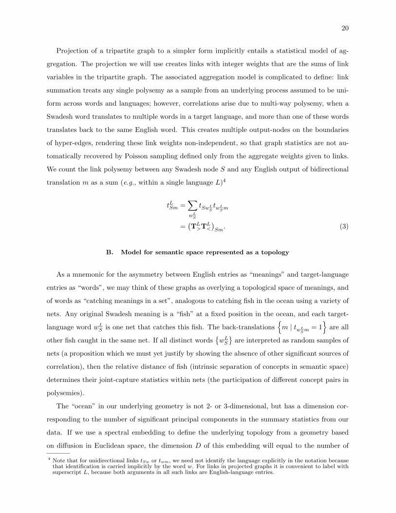
20
Projection of a tripartite graph to a simpler form implicitly entails a statistical model of ag-
gregation. The projection we will use creates links with integer weights that are the sums of link
variables in the tripartite graph. The associated aggregation model is complicated to define: link
summation treats any single polysemy as a sample from an underlying process assumed to be uni-
form across words and languages; however, correlations arise due to multi-way polysemy, when a
Swadesh word translates to multiple words in a target language, and more than one of these words
translates back to the same English word. This creates multiple output-nodes on the boundaries
of hyper-edges, rendering these link weights non-independent, so that graph statistics are not au-
tomatically recovered by Poisson sampling defined only from the aggregate weights given to links.
We count the link polysemy between any Swadesh node S and any English output of bidirectional
translation m as a sum (e.g., within a single language L)4
tLSm =∑wLS
tSwLStwLSm
=(TL>TL
<
)Sm. (3)
B. Model for semantic space represented as a topology
As a mnemonic for the asymmetry between English entries as “meanings” and target-language
entries as “words”, we may think of these graphs as overlying a topological space of meanings, and
of words as “catching meanings in a set”, analogous to catching fish in the ocean using a variety of
nets. Any original Swadesh meaning is a “fish” at a fixed position in the ocean, and each target-
language word wLS is one net that catches this fish. The back-translations{m | twLSm = 1
}are all
other fish caught in the same net. If all distinct words{wLS}
are interpreted as random samples of
nets (a proposition which we must yet justify by showing the absence of other significant sources of
correlation), then the relative distance of fish (intrinsic separation of concepts in semantic space)
determines their joint-capture statistics within nets (the participation of different concept pairs in
polysemies).
The “ocean” in our underlying geometry is not 2- or 3-dimensional, but has a dimension cor-
responding to the number of significant principal components in the summary statistics from our
data. If we use a spectral embedding to define the underlying topology from a geometry based
on diffusion in Euclidean space, the dimension D of this embedding will equal to the number of
4 Note that for unidirectional links tSw or twm, we need not identify the language explicitly in the notation becausethat identification is carried implicitly by the word w. For links in projected graphs it is convenient to label withsuperscript L, because both arguments in all such links are English-language entries.

21
English-language entries recovered in the total sample, and a projection such as multi-dimensional
scaling may be used to select a smaller number of dimensions [11, 12]. In this embedding, diffusion
is isotropic and all “nets” are spherical. More generally, we could envision a lower-dimensional
“ocean” of meanings, and consider nets as ellipsoids characterized by eccentricity and principal
directions as well as central locations. This picture of the origin of polysemy from an inherent
semantic topology is illustrated in Fig. 5, and explained in further detail in the next section.
heatMOON
SUNmonth
gooypah
gyemk
wí
áŋpawí
satellite
moonlightluna
Red: Coast_TsimshianBlue: LakhotaGreen: Spanish
FIG. 5. Hypothetical word-meaning and meaning-meaning relationships using a subset of the data fromFig. 4. In this relation, translation and back-translation across different languages reveal polysemies throughwhich we measure a distance between one concept and another concept.
1. Interpretation of the model into network representation
For an example, consider the projection of the small set of data shown in Fig. 4 (b) and (c).
Words in L = Coast Tsimshian are colored red. For these, we find S = MOON is connected to
m = MOON via the three wLS values gyemgmaatk, gooypah, and gyemk. tCoast TshimshianMOON MOON is, hence,
3, whereas tCoast TshimshianSUN heat = 1 (via gyemk). From the words in L = Lakhota, colored blue in
Fig. 4(c), we see that again tLakhotaMOON MOON = 3, while tLakhotaSUN heat = 0 because there is no polysemy between
these entries in Lakhota.
Diffusion models of projection, which might be of interest of diachronic meaning shift in his-
torical linguistics, is mediated by polysemous intermediates, suggest alternative choices of pro-
jection as well. Instead of counting numbers of polysemes∣∣{wLS}∣∣ between some S and a given
m, a link might be labeled with the share of polysemy of S that goes to that m. This weight-
ing gives tCoast TshimshianMOON MOON = 3/6, because only gyemgmaatk, gooypah, and gyemk are in com-
mon out of 6 and tCoast TshimshianMOON heat = 1/6, because only gyemk is associated out of six polysemes

22
between MOON and heat. In the interpretation of networks as Markov chains of diffusion pro-
cesses, this weight gives the (normalized) probability of transition to m when starting from S, as
tLSm =(∑
wLStSwLS
twLSm
)/(∑
m′∑
w′LStSw′L
Stw′L
Sm′
).
We may return to the analogy of catching fish in a high-dimensional sea, which is the underlying
(geometric or topological) semantic space, referring to Fig. 5. Due to the high dimensionality of
this sea, whether any particular fish m is caught depends on both the position and the angle with
which the net are cast. When the distance between S and m is very small, the angle may matter
little. A cast at a slightly different angle, if it caught S, would again catch m as well. If, instead,
m is far from the center of a net cast to catch S, only for a narrow range of angles will both S and
m be caught. An integer-weighted network measures the number of successes in catching the fish
m as a proxy for relative distance from S. The fractionally-weighted network allows us to consider
the probability of success of catching any fish other than S. If we cast a net many times but only
one succeeds in producing a polysemy, we should think that other meanings m are all remote from
S. Under a fractional weighting, the target language and the English Swadesh categorization may
have different rates of sampling, which appear in the translation dictionary. Our analysis uses
primarily the integer-weighted network.
2. Beyond the available sample data
In the representation of the fine-grained graph as a directed, bipartite graph, English words S
and m, and target-language words w, are formally equivalent. The asymmetry in their roles comes
only from the asymmetry in our sampling protocol over instances of translation. An ideal, fully
symmetric dataset might contain translations between all pairs of languages (L,L′). In such a
dataset, polysemy with respect to any language L could be obtained by an equivalent projection of
all languages other than L. A test for the symmetry of the initial words in such a dataset can come
from projecting out all intermediate languages other than L and L′, and comparing the projected
links from L to L′ through other intermediate languages, against the direct translation dictionary.
A possible area for future work from our current dataset (since curated all-to-all translation will not
be available in the foreseeable future), is to attempt to infer the best approximate translation maps,
e.g. between Coast Tsimshian and Lakhota, through an intermediate sum TCoast Tsimshian< TLakhota
>
analogous to Eq. (3), as a measure of the overlap of graphs GCoast Tsimshian and GLakhota.

23
EARTH/SOIL
DUSTASHES
SAND SMOKE
CLOUD(S)
SKY
DAY/DAYTIME
SUNMOON
STAR
YEAR
MOUNTAIN
STONE/ROCK
SALTSEA/OCEAN
WATER
LAKE
RIVERFIRE
FIG. 6. Connectance graph of Swadesh meanings excluding non-Swadesh English words.
C. The aggregated network of meanings
The polysemy networks of 81 languages, constructed in the previous subsection, are aggregated
into one network structure as shown in Fig. 2 in the main text. Two types of nodes are distinguished
by the case of the label on each node. All-capital labels indicate Swadesh words while all-lowercase
indicate non-Swadesh words. The width of each link is the number of polysemes joining the two
meanings at its endpoints, including in this count the sum of all synonyms within each target
language that reproduce the same polysemy. For example, the thick link between SKY and heaven
implies the existence of the largest number of distinct polysemes between these two compared to
those between any two other entries in the graph.
D. Synonymous polysemy: correlations within and among languages
Synonymous polysemy provides the first, in a series of tests that we will perform, to determine
whether the aggregate graph generated by addition of polysemy-links is a good summary statistic
for the process of word-meaning pairing in actual languages that leads to polysemy. The null model
for sampling from the aggregate graph is that each word from a some Swadesh entry S has a fixed
probability to be polysemous with a given meaning entry m, independent of the presence or absence
of any other polysemes of S with m in the same language. Violations of the null model include
excess synonymous polysemy (suggesting, in our picture of an underlying semantic space, that the
“proximity” of meanings is in part dynamically created by formation of polysemies, increasing their
likelihood of duplication), or deficit synonymous polysemy (suggesting that languages economize

24
0 10 20 30 40 50 60
1.0
1.1
1.2
1.3
1.4
1.5
FIG. 7. The number of synonymous polysemies within a language is correlated with the number of languagescontaining a given polysemy. The horizontal axis indicates the number of languages (out of 81) in which aSwadesh entry S is polysemous with a given meaning m for meanings found to be polysemous in at least twolanguages. The vertical axis indicates the average number of synonymous polysemies per language in whichthe polysemous meaning is represented. Circle areas are proportional to the number of meanings m overwhich the average was taken. The red line represents the least-squares regression over all (non-averaged)data and has slope and intercept of 0.0029 and 1.05, respectively.
on the semantic scope of words by avoiding duplications).
The data presented in Fig. 7 shows that if a given polysemy is represented in more languages, it
is also more likely to be captured by more than one word within a given language. This is consistent
with a model in which proximity relationships among meanings are preexisting. Models in which
the probability of a synonymous polysemy was either independent of the number of polysemous
languages (corresponding to a slope of zero in Fig. 7) or quadratic in the number of languages were
rejected by both AIC and BIC tests.
We partitioned the synonymous polysemy data and performed a series of Mann-Whitney U
tests. We partitioned all polysemies according to the following scheme: a polysemy was a member
of the set cs,p if the language contained the number of polysemies, p, for the given Swadesh word,
s of which shared this polysemous meaning. For each category, we constructed a list Ds,p of the
numbers of languages in which each polysemous meaning in the set cs,p is found. We then tested
all pairs of Ds1,p and Ds2,p for whether they could have been drawn from the same distribution.

25
D0,1 D1,1 0.167 2.53× 10−433
D0,2 D1,2 0.333 1.08× 10−170
D0,2 D2,2 0.0526 1.39× 10−56
D1,2 D2,2 0.158 2.10× 10⁻¹⁴
D0,3 D1,3 0.500 7.18× 10−44
D0,3 D2,3 0.167 1.11× 10⁻²⁸
D0,3 D3,3 0.0222 4.81× 10⁻⁹
D1,3 D2,3 0.333 6.50× 10⁻⁵
D1,3 D2,3 0.0444 4.53× 10⁻⁵
D2,3 D3,3 0.133 9.28× 10⁻⁴
D0,4 D1,4 1.00 3.15× 10⁻¹⁷
D0,4 D2,4 0.0714 1.86× 10⁻¹³
D0,4 D3,4 0.0667 5.63× 10⁻⁵
D1,4 D2,4 0.0714 7.66× 10⁻⁴
D1,4 D3,4 0.0667 0.084
D2,4 D3,4 0.993 1.0
D0,5 D1,5 0.143 1.03× 10⁻²⁷
D0,5 D2,5 0.182 6.20× 10⁻⁷
D0,5 D3,5 0.0323 5.09× 10⁻⁶
D1,5 D2,5 1.27 0.35
D1,5 D3,5 0.226 0.15
D2,5 D3,5 0.177 0.06
D0,6 D1,6 1.00 0.15
D0,6 D2,6 0.0247 1.44× 10⁻⁵
D1,6 D2,6 0.0247 0.06
D0,7 D1,7 1.00 0.20
In most comparisons, the null hypothesis that the two lists were drawn from the same dis-
tribution was strongly rejected, always in the direction where the list with the larger number of
synonymous polysemies (larger values of s) contained larger numbers, meaning that those poly-
semies were found in more different languages. For a few of the comparisons, the null hypothesis
was not rejected, corresponding to those cases where one or both lists included a small number of
entries (< 10).
26
The table II D shows all comparisons for lists of greater than length one. The first two columns
indicate which two lists are being compared. The third column gives the ratio of the median values
of the two lists, with values less than one indicating that the median of the list in the column one
is lower than the median of the list in the column two.
We return to demonstrate a slight excess of probability to include individual entries in poly-
semies, in Sec. IV.
E. Node degree and link presence/absence data
The goodness of this graph as a summary statistic, and the extent to which the heterogeneity of
its node degree and the link topology reflect universals in the sense advocated by Greenberg [13],
may be defined as the extent to which individual language differences are explained as fluctuations
in random samples. We begin systematic tests of the goodness of the aggregate graph with the
degrees of its nodes, a coarse-grained statistic that is most likely to admit the null model of
random sampling, but which also has the best statistical resolution among the observables in our
data. These tests may later be systematically refined by considering the presence/absence statistics
of the set of polysemy links, their covariances, or higher-order moments of the network topology.
At each level of refinement we introduce a more restrictive test, but at the same time we lose
statistical power because the number of possible states grows faster than the data in our sample.
We let nLm denote the degree of meaning m—defined as the sum of weights of links to m—
in language L. Here m may stand for either Swadesh or non-Swadesh entries ({S} ⊂ {m}).
nm ≡∑
L nLm is then the degree of meaning m in the aggregated graph of Fig. 2 (main text),
shown in a rank-size plot in Fig. 3. N ≡∑
m nm =∑
m,L nLm denotes the sum of all link weights
in the aggregated graph.
F. Node degree and Swadesh meanings
The Swadesh list was introduced to provide a priority for the use of lexical items, which favored
universality, stability, and some notion of “core” or “basic” vocabulary. Experience within historical
linguistics suggests qualitatively that it satisfies these criteria well, but the role of the Swadesh
list within semantics has not been studied with quantitative metrics. We may check the degree to
which the items in our basic list are consistent with a notion of core vocabulary by studying their
position in the rank-size distribution of Fig. 4 in the main text.
27
Our sampling methodology naturally places the starting search words (capitalized black char-
acters) high in the distribution, such as EARTH/SOIL, WATER and DAY/DAYTIME with more than
100 polysemous words, because they are all connected to other polysemes produced by polysemy
sampling. Words that are not in the original Swadesh list, but which are uncovered as polysemes
(red), are less fully sampled. They show high degree only if they are connected to multiple Swadesh
entries.5 These derived polysemes fall mostly in the power-law tail of the rank-size distribution in
Fig. 3. The few entries of high degree serve as candidates for inclusion in an expanded Swadesh
list, on the grounds that they are frequently recovered in basic vocabulary. Any severe violation
of the segregation of Swadesh from non-Swadesh entries (hence, the appearance of many derived
polysemes high in the rank-size distribution) would have indicated that the Swadesh entries were
embedded in a larger graph with high clustering coefficient, and would have suggested that the
low-ranking Swadesh words were not statistically favored as starting points to sample a semantic
network.6
III. UNIVERSAL STRUCTURE: CONDITIONAL DEPENDENCE
We performed an extensive range of tests to determine whether language differences in the dis-
tribution of 1) the number of polysemies, 2) the number of meanings (unweighted node degree),
and 3) the average proximity of meanings (weighted node degree, or “strength”) are correlated
with language relatedness, or with geographic or cultural characteristics of the speaker popula-
tions, including the presence or absence of a writing system. The interpretation is analogous to
that of population-level gene frequencies in biology. Language differences that covary with relat-
edness disfavor the Greenbergian view of typological universals of human language, and support a
Whorfian view that most language differences are historically contingent and recur due to vertical
transmission within language families. Differences that covary with cultural or geographical param-
eters suggest that language structure responds to extra-linguistic conditions instead of following
universal endogenous constraints. We find no significant regression of the patterns in our degree
distribution on any cladistic, cultural, or geographical parameters. At the same time, we found
single-language degree distributions consistent with a model of random sampling (defined below),
suggesting that the degree distribution of polysemies is an instance of a Greenbergian universal.
Ruling out dummy variables of clade and culture has a second important implication for studies
5 Note that two non-Swadesh entries cannot be linked to each other, even if they appear in a multi-way polysemy,because our protocol for projecting hypergraphs to simple graphs only generates links between the (Swadesh)inputs and the outputs of bidirectional translation.
6 With greater resources, a bootstrapping method to extend the Swadesh list by following second- and higher-orderpolysemes could provide a quantitative measure of the network position of the Swadesh entries among all relatedwords.
28
of this kind. We chose to collect data by hand from printed dictionaries, foregoing the sample
size and speed of the many online language resources now available, to ensure that our sample
represents the fullest variation known among languages. Online dictionaries and digital corpora
are dominated by a few languages from developed countries, with long-established writing systems
and large speaker populations, but most of these fall within a small number of European or Asian
language families. Our demonstration that relatedness does not produce a strong signal in the
parameters we have measured opens the possibility of more extensive sampling from digital sources.
We note two caveats regarding such a program, however. First, languages for this study were
selected to maximize phylogenetic distance, with no two languages being drawn from the same
genus. It is possible that patterns of polysemy could be shared among more closely related groups
of languages. Second, the strength of any phylogenetic signal might be expected to vary across
semantic domains, so any future analysis will need to be accompanied by explicit universality tests
like those performed here.
A. Comparing semantic networks between language groups
We performed several tests to see if the structure of the polysemy network depends, in a sta-
tistically significant way, on typological features, including the presence or absence of a literary
tradition, geography, topography, and climate. The geographical information is obtained from the
LAPSyD database [14]. We choose the climate categories as the major types A (Humid), B (Arid),
and C–E (Cold) from the Koppen-Geiger climate classification [15], where C–E have been merged
since each of those had few or no languages in our sample. We list the typological features that
are tested, and the numbers of languages for each feature shown in parentheses in the table III
1. Mantel test
Given a set S of languages, we define a weighted graph between English words as shown in
Fig. 2 in the main text. Each matrix entry Aij is the total number of foreign words, summed over
all languages in S, that can be translated or back-translated to or from both ith and j. From
this network, we find the commute distance between the vertices. The commute distance is the
expected number of steps a random walker needs to take to go from one vertex to another [16]. It
is proportional to the more commonly used resistance distance by a proportionality factor of the
sum of all resistances (inverse link weights) in the network.
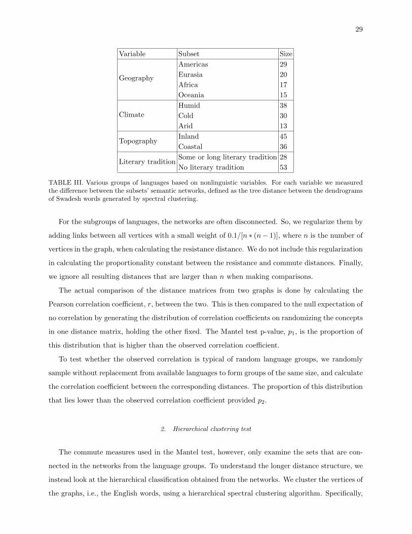
29
Variable Subset Size
Geography
Americas 29
Eurasia 20
Africa 17
Oceania 15
ClimateHumid 38
Cold 30
Arid 13
TopographyInland 45
Coastal 36
Literary traditionSome or long literary tradition 28
No literary tradition 53
TABLE III. Various groups of languages based on nonlinguistic variables. For each variable we measuredthe difference between the subsets’ semantic networks, defined as the tree distance between the dendrogramsof Swadesh words generated by spectral clustering.
For the subgroups of languages, the networks are often disconnected. So, we regularize them by
adding links between all vertices with a small weight of 0.1/[n ∗ (n− 1)], where n is the number of
vertices in the graph, when calculating the resistance distance. We do not include this regularization
in calculating the proportionality constant between the resistance and commute distances. Finally,
we ignore all resulting distances that are larger than n when making comparisons.
The actual comparison of the distance matrices from two graphs is done by calculating the
Pearson correlation coefficient, r, between the two. This is then compared to the null expectation of
no correlation by generating the distribution of correlation coefficients on randomizing the concepts
in one distance matrix, holding the other fixed. The Mantel test p-value, p1, is the proportion of
this distribution that is higher than the observed correlation coefficient.
To test whether the observed correlation is typical of random language groups, we randomly
sample without replacement from available languages to form groups of the same size, and calculate
the correlation coefficient between the corresponding distances. The proportion of this distribution
that lies lower than the observed correlation coefficient provided p2.
2. Hierarchical clustering test
The commute measures used in the Mantel test, however, only examine the sets that are con-
nected in the networks from the language groups. To understand the longer distance structure, we
instead look at the hierarchical classification obtained from the networks. We cluster the vertices of
the graphs, i.e., the English words, using a hierarchical spectral clustering algorithm. Specifically,
30
we assign each word i a point in Rn based on the ith components of the eigenvectors of the n× n
weighted adjacency matrix, where each eigenvector is weighted by the square of its eigenvalue.
We then cluster these points with a greedy agglomerative algorithm, which at each step merges
the pair of clusters with the smallest squared Euclidean distance between their centers of mass.
This produces a binary tree or dendrogram, where the leaves are English words, and internal nodes
correspond to groups and subgroups of words. We obtained these for all 826 English words, but
for simplicity we we show results here for the 22 Swadesh words.
Doing this where S is the set of all 81 languages produces the dendrogram shown in Fig. 8.
We applied the same approach where S is a subgroup of the 81 languages, based on nonlinguistic
variables such as geography, topography, climate, and the presence or absence of a literary tradition.
These groups are shown, along with the number of languages in each, in Table III.
For each nonlinguistic variable, we measured the difference between the semantic network for
each pair of language groups, defined as the distance between their dendrograms. We used two
standard tree metrics taken from the phylogenetic literature. The triplet distance Dtriplet [17, 18]
is the fraction of the(n3
)distinct triplets of words that are assigned a different topology in the two
trees: that is, such that the trees disagree as to which pair of these three words is more closely
related to each other than to the third. The Robinson-Foulds distance DRF [19] is the number
of “cuts” on which the two trees disagree, where a cut is a separation of the leaves into two sets
resulting from removing an edge of the tree.
We then performed two types of bootstrap experiments, comparing these distances to those
one would expect under the null hypotheses. First we considered the hypothesis that there is no
underlying notion of relatedness between senses—for instance, that every pair of words is equally
likely to be siblings in the dendrogram. If this were true, then the dendrograms of each pair of
groups would be no closer than if we permuted the senses on their leaves randomly (while keeping
the structure of the dendrograms the same). Comparing the actual distance between each pair of
groups to the resulting distribution gives the p-values, labeled p1, shown in Figure 3 in the main
text. These p-values are small enough to decisively reject the null hypothesis; indeed, for most
pairs of groups the Robinson-Foulds distance is smaller than that observed in any of the 1000
bootstrap trials, making the p-value effectively zero. This gives overwhelming evidence that the
semantic network has universal aspects, applying across language groups: for instance, in every
group we tried, SEA/OCEAN and SALT are more related than either is to SUN.
In the second type of bootstrap experiment, the null hypothesis is that the nonlinguistic variables
have no effect on the semantic network, and that the differences between language groups simply

31
STAR
YEAR
WIND
SKY
NIGHT
CLOUDHSLSMOKE
SUN
DAYêDAYTIMEMOON
SEAêOCEANLAKE
RIVER
WATER
SALT
MOUNTAIN
STONEêROCKFIRE
DUST
ASHHESLEARTHêSOILSAND
FIG. 8. The dendrogram of Swadesh words generated from spectral clustering on the polysemy networktaken over all 81 languages. The three largest groups are highlighted; roughly speaking, they compriseearth-related, water-related, and sky-related concepts.
result from random sampling: for instance, that the distance between the dendrograms for the
Americas and Eurasia is what one would expect from any disjoint subsets S1, S2 of the 81 languages
of sizes |S1| = 29 and |S2| = 20 respectively. To test this, we generate random pairs of disjoint
subsets with the same sizes as the groups in question, and measure the resulting distribution of
distances. The resulting p-values are labeled p2 in Table 1. These p-values are not small enough
to reject the null hypothesis. Thus, at least given the current data set, it does not appear that
these nonlinguistic variables have a statistically significant effect on the semantic network—further
supporting our thesis that it is, at least in part, universal.
For illustration, in Fig. 3 (main text) we compare the triplet distance between the dendrograms
for Americas and Oceania with the distributions from the two bootstrap experiments. These two
groups are closer than less than 2% of the trees where senses have been permuted randomly, but
38% of the random pairs of subsets of size 29 and 15 are farther away. Using a p-value of 0.05 as
the usual threshold, we can reject the hypothesis that these two groups have no semantic structure
in common; moreover, we cannot reject the hypothesis that the differences between them are due
to random sampling rather than geographic differences.

32
B. Statistical significance
The p-values reported in Fig. 3 have to be corrected for multiple tests. Eleven independent
comparisons are performed for each of the metrics, so a low p-value is occasionally expected simply
by chance. In fact, under the null hypothesis, a column will contain a single p = 0.01 by chance
about 10% of the time. To correct for this, one can employ a Bonferroni correction [20] leading to
a significance threshold of 0.005 for each of the 11 tests, corresponding to a test size of p = 0.05.
Most of the comparisons in the p1 columns for r and DRF are comfortably are below this threshold,
implying that the networks obtained from different language groups are indeed significantly more
similar than comparable random networks.
A Bonferroni correction, however, is known to be aggressive: it controls the false positive er-
ror rate but leads to many false negatives [21], and is not appropriate for establishing the lack
of significance for the p2 columns. The composite hypothesis that none of the comparisons are
statistically significant leads to the predictions that the corresponding p-values are uniformly dis-
tributed between 0 and 1. One can, therefore, test the obtained p-values against this expected
uniform distribution. We performed a Kolmogorov-Smirnov test for uniformity for each column
of the table. This composite p-value is about 0.11 and 0.27 for the p2 columns corresponding to
Dtriplet and DRF, showing that these columns are consistent with chance fluctuations. The p-value
corresponding to the p2 column for r is about 0.03, evidence that at least one pair of networks
are more dissimilar than expected for a random grouping of languages. This is consistent with the
indication from the Bonferroni threshold as well—the comparison of Americas and Eurasia has a
significant p-value, as possibly also the comparison between Humid and Arid. Removing either of
these comparisons raises the composite p-value to 0.10, showing that such a distribution containing
one low p-value (but not two) would be expected to occur by chance about 10% of the time.
C. Single-language graph size is a significant summary statistic
The only important language-dependent variable not attached to words in the aggregate graph
of Fig. 2 (main text), which is a strongly significant summary statistic for samples, is the total link
weight in the language, nL ≡∑
S nLS . In the next section we will quantify the role of this variable
in producing single-language graphs as samples from the aggregate graph, conditioned on the total
weight of the language.
Whereas we do associate node degree and link weight in the aggregate graph with inherent and
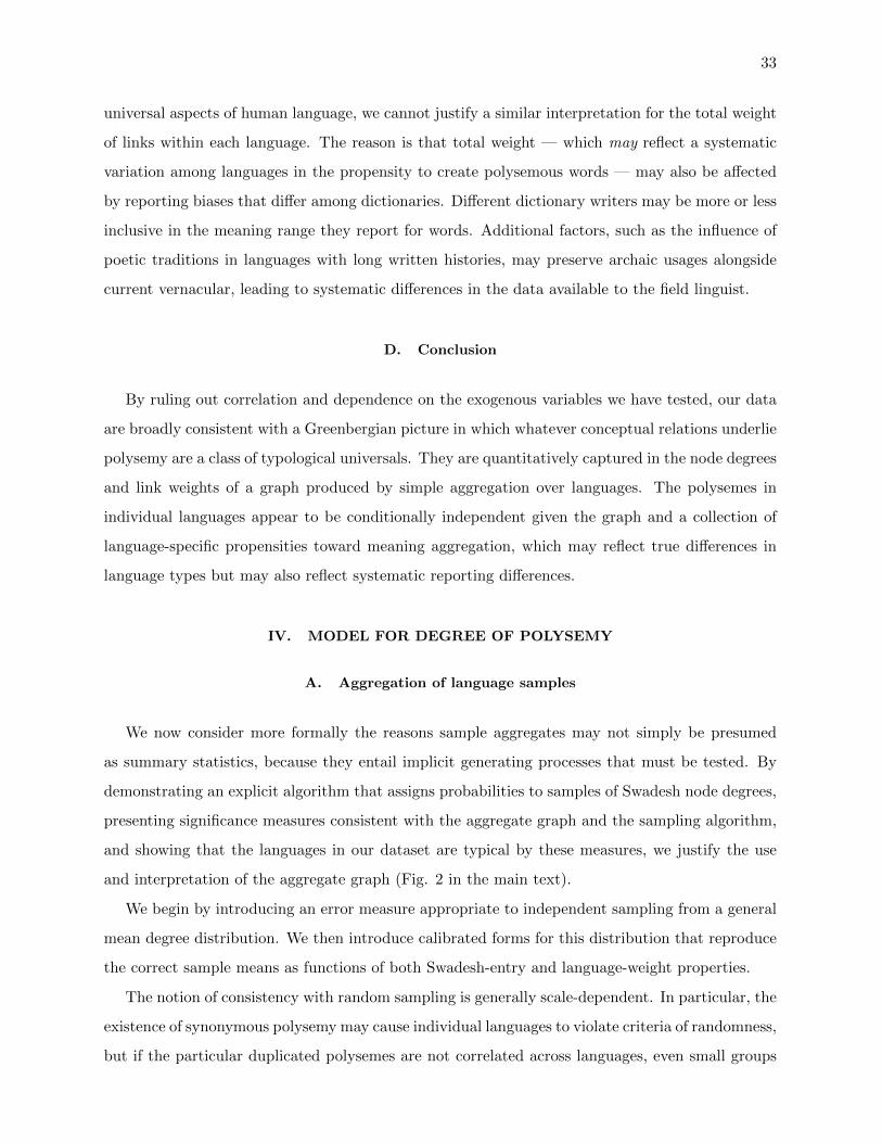
33
universal aspects of human language, we cannot justify a similar interpretation for the total weight
of links within each language. The reason is that total weight — which may reflect a systematic
variation among languages in the propensity to create polysemous words — may also be affected
by reporting biases that differ among dictionaries. Different dictionary writers may be more or less
inclusive in the meaning range they report for words. Additional factors, such as the influence of
poetic traditions in languages with long written histories, may preserve archaic usages alongside
current vernacular, leading to systematic differences in the data available to the field linguist.
D. Conclusion
By ruling out correlation and dependence on the exogenous variables we have tested, our data
are broadly consistent with a Greenbergian picture in which whatever conceptual relations underlie
polysemy are a class of typological universals. They are quantitatively captured in the node degrees
and link weights of a graph produced by simple aggregation over languages. The polysemes in
individual languages appear to be conditionally independent given the graph and a collection of
language-specific propensities toward meaning aggregation, which may reflect true differences in
language types but may also reflect systematic reporting differences.
IV. MODEL FOR DEGREE OF POLYSEMY
A. Aggregation of language samples
We now consider more formally the reasons sample aggregates may not simply be presumed
as summary statistics, because they entail implicit generating processes that must be tested. By
demonstrating an explicit algorithm that assigns probabilities to samples of Swadesh node degrees,
presenting significance measures consistent with the aggregate graph and the sampling algorithm,
and showing that the languages in our dataset are typical by these measures, we justify the use
and interpretation of the aggregate graph (Fig. 2 in the main text).
We begin by introducing an error measure appropriate to independent sampling from a general
mean degree distribution. We then introduce calibrated forms for this distribution that reproduce
the correct sample means as functions of both Swadesh-entry and language-weight properties.
The notion of consistency with random sampling is generally scale-dependent. In particular, the
existence of synonymous polysemy may cause individual languages to violate criteria of randomness,
but if the particular duplicated polysemes are not correlated across languages, even small groups

34
of languages may rapidly converge toward consistency with a random sample. Indeed the section
II D shows the independence of synonymous polysemy. Therefore, we do not present only a single
acceptance/rejection criterion for our dataset, but rather show the smallest groupings for which
sampling is consistent with randomness, and then demonstrate a model that reproduces the excess
but uncorrelated synonymous polysemy within individual languages.
B. Independent sampling from the aggregate graph
Figure 2 (main text) treats all words in all languages as independent members of an unbiased
sample. To test the appropriateness of the aggregate as a summary statistic, we ask: do random
samples, with link numbers equal to those in observed languages, and with link probabilities
proportional to the weights in the aggregate graph, yield ensembles of graphs within which the
actual languages in our data are typical?
1. Statistical tests
The appropriate summary statistic to test for typicality, in ensembles produced by random
sampling (of links or link-ends) is the Kullback-Leibler (KL) divergence of the sample counts from
the probabilities with which the samples were drawn [22, 23]. This is because the KL divergence
is the leading exponential approximation (by Stirling’s formula) to the log of the multinomial
distribution produced by Poisson sampling.
The appropriateness of a random-sampling model may be tested independently of how the
aggregate link numbers are used to generate an underlying probability model. In this section, we
will first evaluate a variety of underlying probability models under Poisson sampling, and then we
will return to tests for deviations from independent Poisson samples. We first introduce notation:
For a single language, the relative degree (link frequency), which is used as the normalization
of a probability, is denoted as pdataS|L ≡ nLS/nL, and for the joint configuration of all words in all
languages, the link frequency of a single entry relative to the total N will be denoted pdataSL ≡
nLS/N =(nLS/n
L) (nL/N
)≡ pdataS|L p
dataL .
Corresponding to any of these, we may generate samples of links to define the null model for
a random process, which we denote nLS , nL, etc. We will generally use samples with exactly the
same number of total links N as the data. The corresponding sample frequencies will be denoted
by psampleS|L ≡ nLS/nL and psample
SL ≡ nLS/N =(nLS/n
L) (nL/N
)≡ psample
S|L psampleL , respectively.

35
Finally, the calibrated model, which we define from properties of aggregated graphs, will be
the prior probability from which samples are drawn to produce p-values for the data. We denote
the model probabilities (which are used in sampling as “true” probabilities rather than sample
frequencies) by pmodelS|L , pmodel
SL , and pmodelL .
For nL links sampled independently from the distribution psampleS|L for language L, the multinomial
probability of a particular set{nLS}
may be written, using Stirling’s formula to leading exponential
order, as
p({nLS}| nL
)∼ e−n
LD(psampleS|L
∥∥∥pmodelS|L
)(4)
where the Kullback-Leibler (KL) divergence [22, 23]
D(psampleS|L
∥∥∥ pmodelS|L
)≡∑S
psampleS|L log
psampleS|L
pmodelS|L
. (5)
For later reference, note that the leading quadratic approximation to Eq. (5) is
nLD(psampleS|L
∥∥∥ pmodelS|L
)≈ 1
2
∑S
(nLS − nLpmodel
S|L
)2nLpmodel
S|L, (6)
so that the variance of fluctuations in each word is proportional to its expected frequency.
As a null model for the joint configuration over all languages in our set, if N links are drawn
independently from the distribution psampleSL , the multinomial probability of a particular set
{nLS}
is given by
p({nLS}| N)∼ e−ND
(psampleSL
∥∥∥pmodelSL
)(7)
where7
D(psampleSL
∥∥∥ pmodelSL
)≡∑S,L
psampleSL log
(psampleSL
pmodelSL
)
= D(psampleL
∥∥∥ pmodelL
)+∑L
psampleL D
(psampleS|L
∥∥∥ pmodelS|L
).
(8)
7 As long as we calibrate pmodelL to agree with the per-language link frequencies nL/N in the data, the data will
always be counted as more typical than almost-all random samples, and its probability will come entirely from theKL divergences in the individual languages.

36
Multinomial samples of assignments nLS to each of the 22× 81 (Swadesh,Language) pairs, with
N links total drawn from distribution pLSnull
, will produce KL divergences uniformly distributed in
the coordinate dΦ ≡ e−DKLdDKL, corresponding to the uniform increment of cumulative proba-
bility in the model distribution. We may therefore use the cumulative probability to the right of
D(pdataSL
∥∥ pmodelSL
)(one-sided p-value), in the distribution of samples nLS , as a test of consistency of
our data with the model of random sampling.
In the next two subsections we will generate and test candidates for pmodel which are different
functions of the mean link numbers on Swadesh concepts and the total links numbers in languages.
2. Product model with intrinsic property of concepts
In general we wish to consider the consistency of joint configurations with random sampling, as
a function of an aggregation scale. To do this, we will rank-order languages by increasing nL, form
non-overlapping bins of 1, 3, or 9 languages, and test the resulting binned degree distributions
against different mean-degree and sampling models. We denote by⟨nL⟩
the average total link
number in a bin, and by⟨nLS⟩
the average link number per Swadesh entry in the bin. The simplest
model, which assumes no interaction between concept and language properties, makes the model
probability pmodelSL a product of its marginals. It is estimated from data without regard to binning,
as
pproductSL ≡ nSN× nL
N. (9)
The 22× 81 independent mean values are thereby specified in terms of 22 + 81 sample estimators.
The KL divergence of the joint configuration of links in the actual data from this model, under
whichever binning is used, becomes
D(pdataSL
∥∥∥ pmodelSL
)= D
(⟨nLS⟩
N
∥∥∥∥∥nSN⟨nL⟩
N
)(10)
As we show in Fig. 11 below, even for 9-language bins which we expect to average over a large
amount of language-specific fluctuation, the product model is ruled out at the 1% level.
We now show that a richer model, describing interaction between word and language proper-
ties, accepts not only the 9-language aggregate, but also the 3-language aggregate with a small
adjustment of the language size to which words respond (to produce consistency with word-size
and language-size marginals). Only fluctuation statistics at the level of the joint configuration of
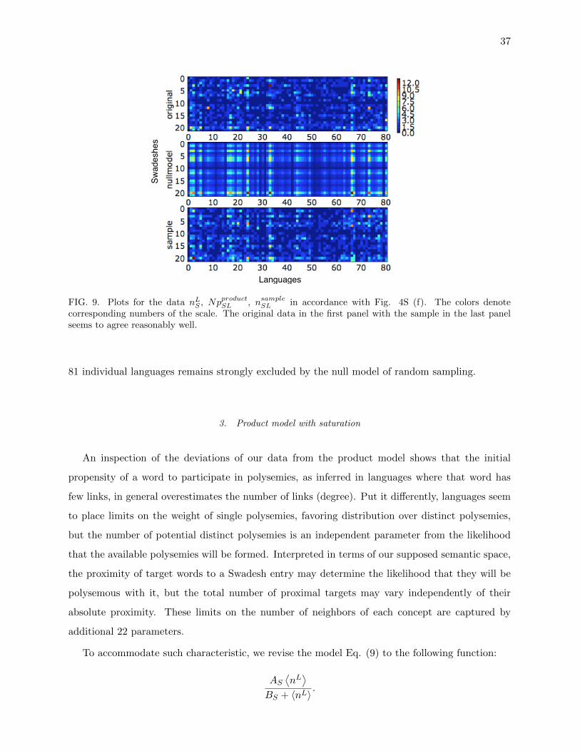
37
Languages
Swadeshes
FIG. 9. Plots for the data nLS , NpproductSL , nsampleSL in accordance with Fig. 4S (f). The colors denotecorresponding numbers of the scale. The original data in the first panel with the sample in the last panelseems to agree reasonably well.
81 individual languages remains strongly excluded by the null model of random sampling.
3. Product model with saturation
An inspection of the deviations of our data from the product model shows that the initial
propensity of a word to participate in polysemies, as inferred in languages where that word has
few links, in general overestimates the number of links (degree). Put it differently, languages seem
to place limits on the weight of single polysemies, favoring distribution over distinct polysemies,
but the number of potential distinct polysemies is an independent parameter from the likelihood
that the available polysemies will be formed. Interpreted in terms of our supposed semantic space,
the proximity of target words to a Swadesh entry may determine the likelihood that they will be
polysemous with it, but the total number of proximal targets may vary independently of their
absolute proximity. These limits on the number of neighbors of each concept are captured by
additional 22 parameters.
To accommodate such characteristic, we revise the model Eq. (9) to the following function:
AS⟨nL⟩
BS + 〈nL〉.

38
0 20 40 60
0
10
20
30
40
0 20 40 600
5
10
15
20
25
<nL>bin
nLS=WATER
nLS=MOON
<nL>bin
FIG. 10. Plots of the saturating function (11) with the parameters given in Table IV, compared to⟨nLS⟩
(ordinate) in 9-language bins (to increase sample size), versus bin-averages⟨nL⟩
(abscissa). Red line is drawnthrough data values, blue is the product model, and green is the saturation model. WATER requires nosignificant deviation from the product model (BWATER/N � 20), while MOON shows the lowest saturationvalue among the Swadesh entries, at BMOON ≈ 3.4.
where degree numbers⟨nLS⟩
for each Swadesh S is proportional to AS and language size, but is
bounded by BS , the number of proximal concepts. The corresponding model probability for each
language then becomes
psatSL =(AS/BS)(nL/N)
1 + nL/BS≡
pSpdataL
1 + pdataL N/BS. (11)
As all BS/N →∞ we recover the product model, with pdataL ≡ nL/N and pS → nS/N .
A first-level approximation to fit parameters AS and BS is given by minimizing the weighted
mean-square error
E ≡∑L
1
〈nL〉∑S
(⟨nLS⟩−
AS⟨nL⟩
BS + 〈nL〉
)2
. (12)
The function (12) assigns equal penalty to squared error within each language bin ∼⟨nL⟩, propor-
tional to the variance expected from Poisson sampling. The fit values obtained for AS and BS do
not depend sensitively on the size of bins except for the Swadesh entry MOON in the case where all
81 single-language bins are used. MOON has so few polysemies, but the MOON/month polysemy
is so likely to be found, that the language Itelman, with only one link, has this polysemy. This point
leads to instabilities in fitting BMOON in single-language bins. For bins of size 3–9 the instability
is removed. Representative fit parameters across this range are shown in Table IV. Examples of
the saturation model for two words, plotted against the 9-language binned degree data in Fig. 10,
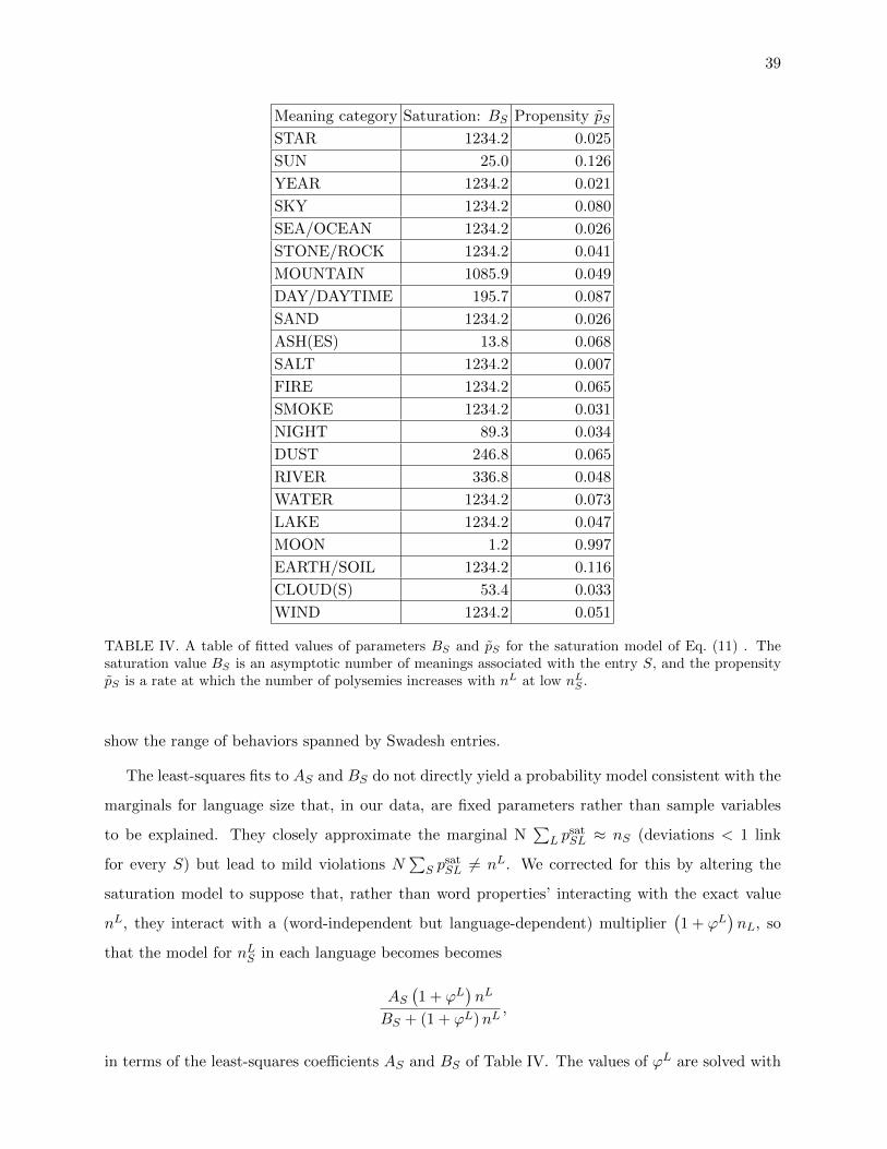
39
Meaning category Saturation: BS Propensity pS
STAR 1234.2 0.025
SUN 25.0 0.126
YEAR 1234.2 0.021
SKY 1234.2 0.080
SEA/OCEAN 1234.2 0.026
STONE/ROCK 1234.2 0.041
MOUNTAIN 1085.9 0.049
DAY/DAYTIME 195.7 0.087
SAND 1234.2 0.026
ASH(ES) 13.8 0.068
SALT 1234.2 0.007
FIRE 1234.2 0.065
SMOKE 1234.2 0.031
NIGHT 89.3 0.034
DUST 246.8 0.065
RIVER 336.8 0.048
WATER 1234.2 0.073
LAKE 1234.2 0.047
MOON 1.2 0.997
EARTH/SOIL 1234.2 0.116
CLOUD(S) 53.4 0.033
WIND 1234.2 0.051
TABLE IV. A table of fitted values of parameters BS and pS for the saturation model of Eq. (11) . Thesaturation value BS is an asymptotic number of meanings associated with the entry S, and the propensitypS is a rate at which the number of polysemies increases with nL at low nLS .
show the range of behaviors spanned by Swadesh entries.
The least-squares fits to AS and BS do not directly yield a probability model consistent with the
marginals for language size that, in our data, are fixed parameters rather than sample variables
to be explained. They closely approximate the marginal N∑
L psatSL ≈ nS (deviations < 1 link
for every S) but lead to mild violations N∑
S psatSL 6= nL. We corrected for this by altering the
saturation model to suppose that, rather than word properties’ interacting with the exact value
nL, they interact with a (word-independent but language-dependent) multiplier(1 + ϕL
)nL, so
that the model for nLS in each language becomes becomes
AS(1 + ϕL
)nL
BS + (1 + ϕL)nL,
in terms of the least-squares coefficients AS and BS of Table IV. The values of ϕL are solved with

40
0.04 0.045 0.05 0.055 0.06 0.065 0.07 0.075 0.08
0
50
100
150
200
250
300
350
400
450
500
DKL(samples || saturation model)
His
tog
ram
co
un
ts
FIG. 11. Kullback-Leibler divergence of link frequencies in our data, grouped into non-overlapping 9-language bins ordered by rank, from the product distribution (9) and the saturation model (11). ParametersAS and BS have been adjusted (as explained in the text) to match the word- and language-marginals. From10,000 random samples nLS , (green) histogram for the product model; (blue) histogram for the saturationmodel; (red dots) data. The product model rejects the 9-language joint binned configuration at the at1% level (dark shading), while the saturation model is typical of the same configuration at ∼ 59% (lightshading).
Newton’s method to produce N∑
S psatSL → nL, and we checked that they preserve N
∑L p
satSL ≈ nS
within small fractions of a link. The resulting adjustment parameters are plotted versus nL for
individual languages in Fig. 12. Although they were computed individually for each L, they form
a smooth function of nL, possibly suggesting a refinement of the product model, but also perhaps
reflecting systematic interaction of small-language degree distributions with the error function (12).
-0.5
-0.4
-0.3
-0.2
-0.1
0
0.1
0.2
0 10 20 30 40 50 60 70
L
nL
ϕ
FIG. 12. Plot of the correction factor ϕL versus nL for individual languages in the probability model usedin text, with parameters BS and pS shown in Table IV. Although ϕL values were individually solved withNewton’s method to ensure that the probability model matched the whole-language link values, the resultingcorrection factors are a smooth function of nL.
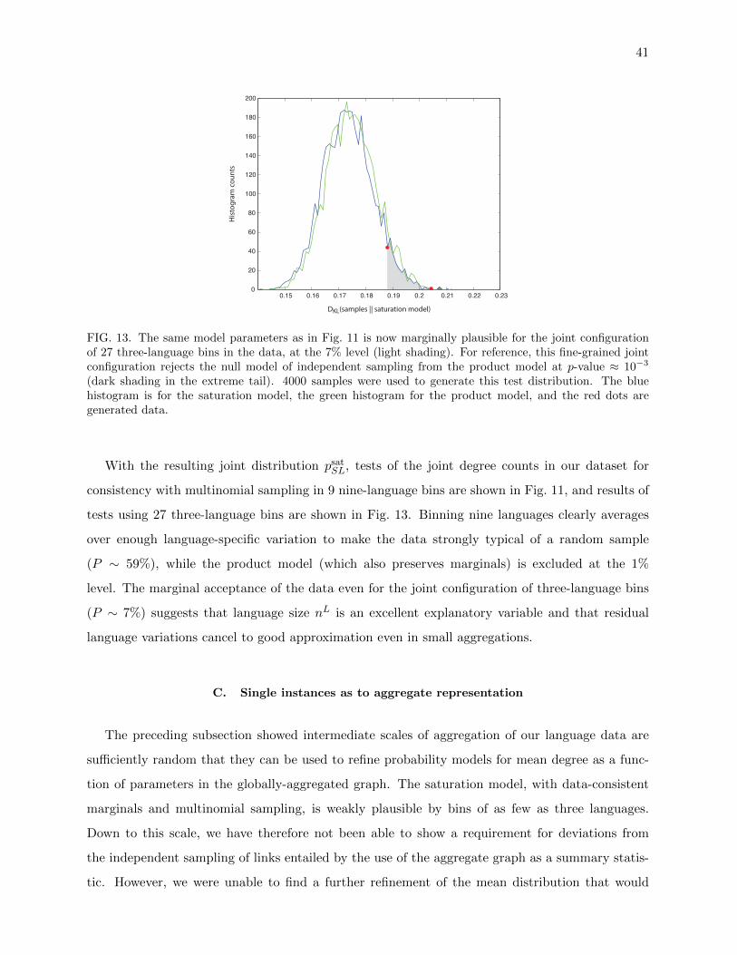
41
0.15 0.16 0.17 0.18 0.19 0.2 0.21 0.22 0.23
0
20
40
60
80
100
120
140
160
180
200
DKL(samples || saturation model)
His
tog
ram
co
un
ts
FIG. 13. The same model parameters as in Fig. 11 is now marginally plausible for the joint configurationof 27 three-language bins in the data, at the 7% level (light shading). For reference, this fine-grained jointconfiguration rejects the null model of independent sampling from the product model at p-value ≈ 10−3
(dark shading in the extreme tail). 4000 samples were used to generate this test distribution. The bluehistogram is for the saturation model, the green histogram for the product model, and the red dots aregenerated data.
With the resulting joint distribution psatSL, tests of the joint degree counts in our dataset for
consistency with multinomial sampling in 9 nine-language bins are shown in Fig. 11, and results of
tests using 27 three-language bins are shown in Fig. 13. Binning nine languages clearly averages
over enough language-specific variation to make the data strongly typical of a random sample
(P ∼ 59%), while the product model (which also preserves marginals) is excluded at the 1%
level. The marginal acceptance of the data even for the joint configuration of three-language bins
(P ∼ 7%) suggests that language size nL is an excellent explanatory variable and that residual
language variations cancel to good approximation even in small aggregations.
C. Single instances as to aggregate representation
The preceding subsection showed intermediate scales of aggregation of our language data are
sufficiently random that they can be used to refine probability models for mean degree as a func-
tion of parameters in the globally-aggregated graph. The saturation model, with data-consistent
marginals and multinomial sampling, is weakly plausible by bins of as few as three languages.
Down to this scale, we have therefore not been able to show a requirement for deviations from
the independent sampling of links entailed by the use of the aggregate graph as a summary statis-
tic. However, we were unable to find a further refinement of the mean distribution that would
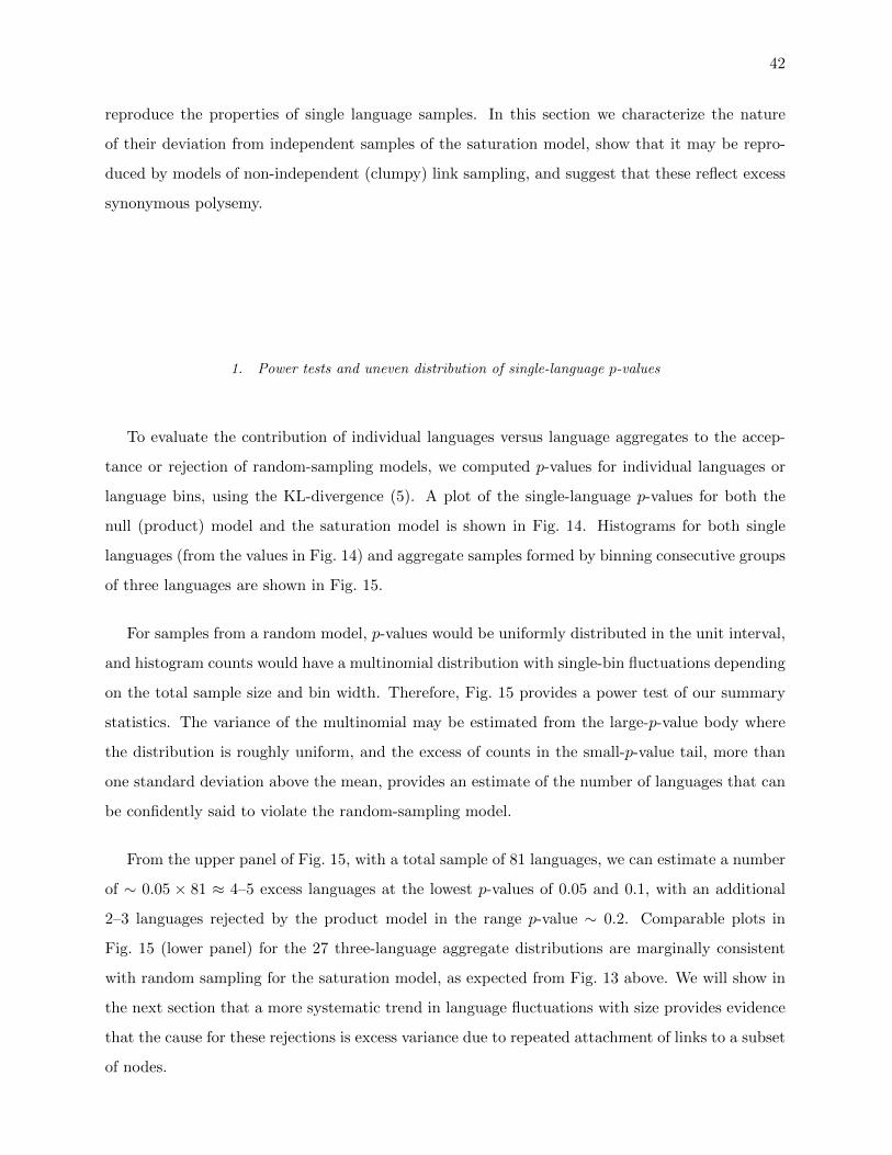
42
reproduce the properties of single language samples. In this section we characterize the nature
of their deviation from independent samples of the saturation model, show that it may be repro-
duced by models of non-independent (clumpy) link sampling, and suggest that these reflect excess
synonymous polysemy.
1. Power tests and uneven distribution of single-language p-values
To evaluate the contribution of individual languages versus language aggregates to the accep-
tance or rejection of random-sampling models, we computed p-values for individual languages or
language bins, using the KL-divergence (5). A plot of the single-language p-values for both the
null (product) model and the saturation model is shown in Fig. 14. Histograms for both single
languages (from the values in Fig. 14) and aggregate samples formed by binning consecutive groups
of three languages are shown in Fig. 15.
For samples from a random model, p-values would be uniformly distributed in the unit interval,
and histogram counts would have a multinomial distribution with single-bin fluctuations depending
on the total sample size and bin width. Therefore, Fig. 15 provides a power test of our summary
statistics. The variance of the multinomial may be estimated from the large-p-value body where
the distribution is roughly uniform, and the excess of counts in the small-p-value tail, more than
one standard deviation above the mean, provides an estimate of the number of languages that can
be confidently said to violate the random-sampling model.
From the upper panel of Fig. 15, with a total sample of 81 languages, we can estimate a number
of ∼ 0.05 × 81 ≈ 4–5 excess languages at the lowest p-values of 0.05 and 0.1, with an additional
2–3 languages rejected by the product model in the range p-value ∼ 0.2. Comparable plots in
Fig. 15 (lower panel) for the 27 three-language aggregate distributions are marginally consistent
with random sampling for the saturation model, as expected from Fig. 13 above. We will show in
the next section that a more systematic trend in language fluctuations with size provides evidence
that the cause for these rejections is excess variance due to repeated attachment of links to a subset
of nodes.

43
0 10 20 30 40 50 60 70 80 90
−4
−3.5
−3
−2.5
−2
−1.5
−1
−0.5
0
log
10
(P)
Language (rank)
FIG. 14. log10(p−value) by KL divergence, relative to 4000 random samples per language, plotted versuslanguage rank in order of increasing nL. Product model (green) shows equal or lower p-values for almostall languages than the saturation model (blue). Three languages – Basque, Haida, and Yoruba – had valuep = 0 consistently across samples in both models, and are removed from subsequent regression estimates.A trend toward decreasing p is seen with increase in nL.
2. Excess fluctuations in degree of polysemy
If we define the size-weighted relative variance of a language analogously to the error term in
Eq. (12), as
(σ2)L ≡ 1
nL
∑S
(nLS − nLpmodel
S|L
)2, (13)
Fig. 16 shows that − log10(p−value) has high rank correlation with(σ2)L
and a roughly linear
regression over most of the range.8 Two languages (Itelmen and Hindi), which appear as large
outliers relative to the product model, are within the main dispersion in the saturation model,
showing that their discrepancy is corrected in the mean link number. We may therefore understand
a large fraction of the improbability of languages as resulting from excess fluctuations of their degree
numbers relative to the expectation from Poisson sampling.
Fig. 17 then shows the relative variance from the saturation model, plotted versus total average
link number for both individual languages and three-language bins. The binned languages show no
significant regression of relative variance away from the value unity for Poisson sampling, whereas
single languages show a systematic trend toward larger variance in larger languages, a pattern that
8 Recall from Eq. (6) that the leading quadratic term in the KL-divergence differs from(σ2
)Lin that it presumes
Poisson fluctuation with variance nLpmodelS|L at the level of each word, rather than uniform variance ∝ nL across
all words in a language. The relative variance is thus a less specific error measure.

44
0 0.1 0.2 0.3 0.4 0.5 0.6 0.7 0.8 0.9 10
0.05
0.1
0.15
0.2
0.25
0.3
0.35
P (bin center)
Fra
ctio
n o
f la
ng
ua
ge
s w
ith
pro
ba
bili
ty P
Unambiguous excesslow-P samples
0 0.1 0.2 0.3 0.4 0.5 0.6 0.7 0.8 0.9 10
0.05
0.1
0.15
0.2
0.25
0.3
0.35
P (bin center)
Fra
ctio
n o
f la
ng
ua
ge
s w
ith
pro
ba
bili
ty P
FIG. 15. (Upper panel) Normalized histogram of p-values from the 81 languages plotted in Fig. 14. Thesaturation model (blue) produces a fraction ∼ 0.05 × 81 ≈ 4–5 languages in the lowest p-values {0.05, 0.1}above the roughly-uniform background for the rest of the interval (shaded area with dashed boundary). Afurther excess of 2–3 languages with p-values in the range [0, 0.2] for the product model (green) reflects thepart of the mismatch corrected through mean values in the saturation model. (Lower panel) Correspondinghistogram of p-values for 27 three-language aggregate degree distributions. Saturation model (blue) is nowmarginally consistent with a uniform distribution, while the product model (green) still shows slight excessof low-p bins. Coarse histogram bins have been used in both panels to compensate for small sample numbersin the lower panel, while producing comparable histograms.
we will show is consistent with “clumpy” sampling of a subset of nodes. The disappearance of
this clumping in binned distributions shows that the clumps are uncorrelated among languages at
similar nL.
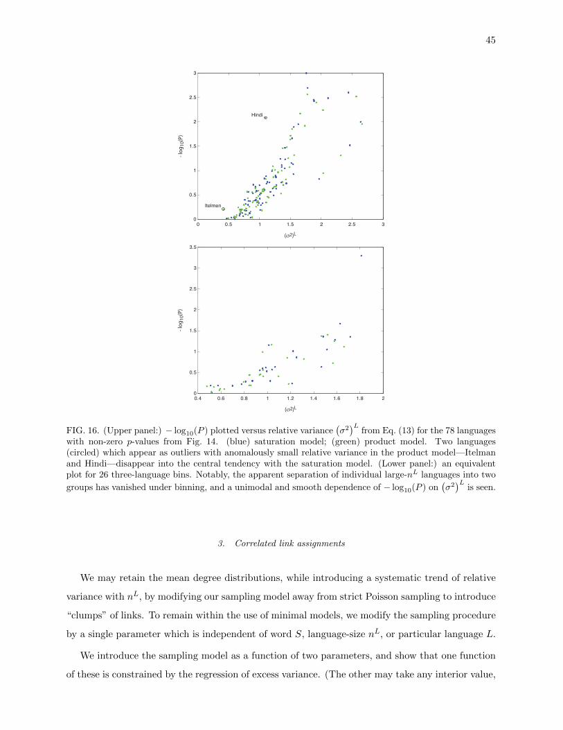
45
0 0.5 1 1.5 2 2.5 3
0
0.5
1
1.5
2
2.5
3
(σ2)L
- lo
g1
0(P
)
Itelmen
Hindi
0.4 0.6 0.8 1 1.2 1.4 1.6 1.8 2
0
0.5
1
1.5
2
2.5
3
3.5
(σ2)L
- lo
g1
0(P
)
FIG. 16. (Upper panel:) − log10(P ) plotted versus relative variance(σ2)L
from Eq. (13) for the 78 languageswith non-zero p-values from Fig. 14. (blue) saturation model; (green) product model. Two languages(circled) which appear as outliers with anomalously small relative variance in the product model—Itelmanand Hindi—disappear into the central tendency with the saturation model. (Lower panel:) an equivalentplot for 26 three-language bins. Notably, the apparent separation of individual large-nL languages into two
groups has vanished under binning, and a unimodal and smooth dependence of − log10(P ) on(σ2)L
is seen.
3. Correlated link assignments
We may retain the mean degree distributions, while introducing a systematic trend of relative
variance with nL, by modifying our sampling model away from strict Poisson sampling to introduce
“clumps” of links. To remain within the use of minimal models, we modify the sampling procedure
by a single parameter which is independent of word S, language-size nL, or particular language L.
We introduce the sampling model as a function of two parameters, and show that one function
of these is constrained by the regression of excess variance. (The other may take any interior value,

46
0 10 20 30 40 50 60 70
0
0.5
1
1.5
2
2.5
3
nL
(σ2
)L
(σ2)L = 0.011938 nL + 0.87167
(σ2)L = 0.0023919 nL + 0.94178
FIG. 17. Relative variance from the saturation model versus total link number nL for 78 languages excludingBasque, Haida, and Yoruba. Least-squares regression are shown for three-language bins (green) and indi-vidual languages (blue), with regression coefficients inset. Three-language bins are consistent with Poissonsampling at all nL, whereas single languages show systematic increase of relative variance with increasingnL.
so we have an equivalence class of models.) In each language, select a number B of Swadesh entries
randomly. Let the Swadesh indices be denoted {Sβ}β∈1,...B. We will take some fraction of the total
links in that language, and assign them only to the Swadeshes whose indices are in this privileged
set. Introduce a parameter q that will determine that fraction.
We require correlated link assignments be consistent with the mean determined by our model
fit, since binning of data has shown no systematic effect on mean parameters. Therefore, for the
random choice {Sβ}β∈1,...B, introduce the normalized density on the privileged links
πS|L ≡pmodelS|L∑B
β=1 pmodelSβ |L
(14)
if S ∈ {Sβ}β∈1,...B and πS|L = 0 otherwise. Denote the aggregated weight of the links in the
privileged set by
W ≡B∑β=1
pSβ |L. (15)
Then introduce a modified probability distribution based on the randomly selected links, in the
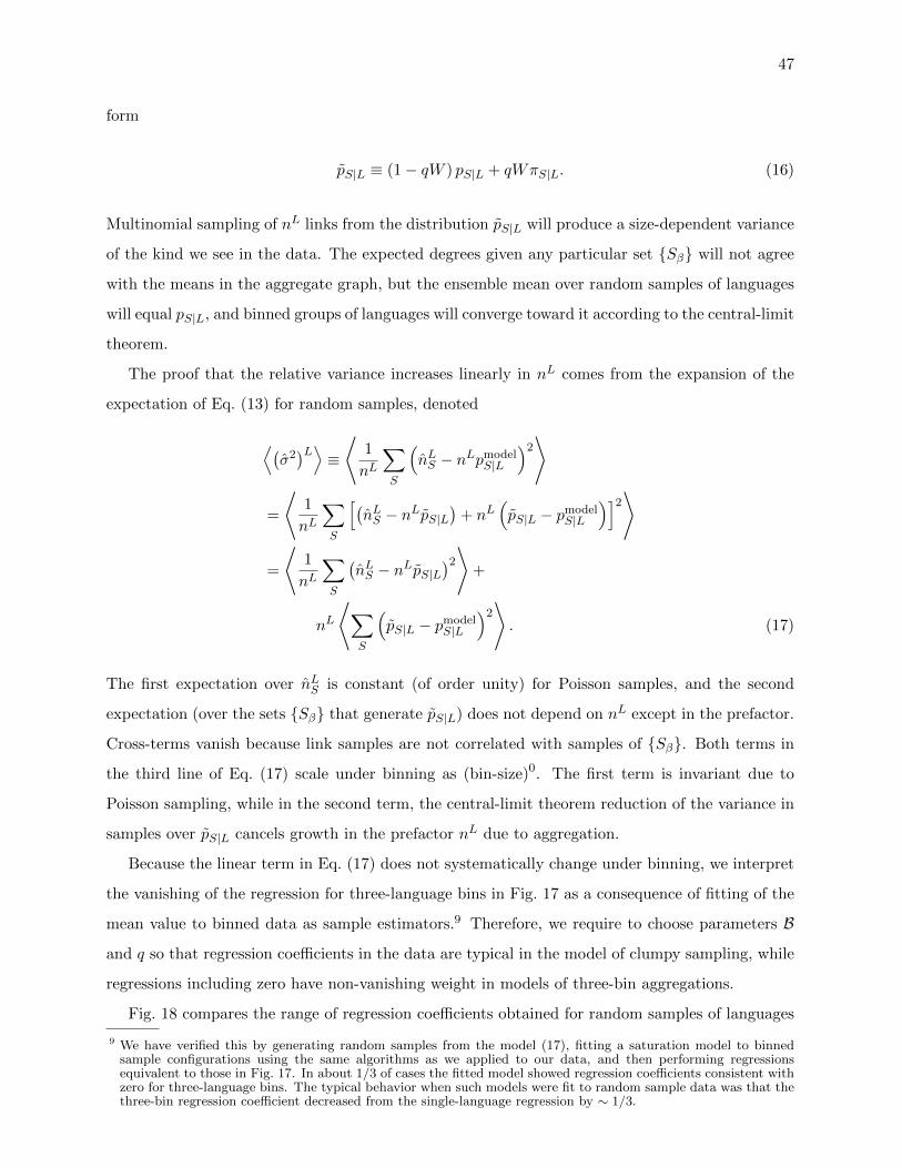
47
form
pS|L ≡ (1− qW ) pS|L + qWπS|L. (16)
Multinomial sampling of nL links from the distribution pS|L will produce a size-dependent variance
of the kind we see in the data. The expected degrees given any particular set {Sβ} will not agree
with the means in the aggregate graph, but the ensemble mean over random samples of languages
will equal pS|L, and binned groups of languages will converge toward it according to the central-limit
theorem.
The proof that the relative variance increases linearly in nL comes from the expansion of the
expectation of Eq. (13) for random samples, denoted
⟨(σ2)L⟩ ≡ ⟨ 1
nL
∑S
(nLS − nLpmodel
S|L
)2⟩
=
⟨1
nL
∑S
[(nLS − nLpS|L
)+ nL
(pS|L − pmodel
S|L
)]2⟩
=
⟨1
nL
∑S
(nLS − nLpS|L
)2⟩+
nL
⟨∑S
(pS|L − pmodel
S|L
)2⟩. (17)
The first expectation over nLS is constant (of order unity) for Poisson samples, and the second
expectation (over the sets {Sβ} that generate pS|L) does not depend on nL except in the prefactor.
Cross-terms vanish because link samples are not correlated with samples of {Sβ}. Both terms in
the third line of Eq. (17) scale under binning as (bin-size)0. The first term is invariant due to
Poisson sampling, while in the second term, the central-limit theorem reduction of the variance in
samples over pS|L cancels growth in the prefactor nL due to aggregation.
Because the linear term in Eq. (17) does not systematically change under binning, we interpret
the vanishing of the regression for three-language bins in Fig. 17 as a consequence of fitting of the
mean value to binned data as sample estimators.9 Therefore, we require to choose parameters B
and q so that regression coefficients in the data are typical in the model of clumpy sampling, while
regressions including zero have non-vanishing weight in models of three-bin aggregations.
Fig. 18 compares the range of regression coefficients obtained for random samples of languages
9 We have verified this by generating random samples from the model (17), fitting a saturation model to binnedsample configurations using the same algorithms as we applied to our data, and then performing regressionsequivalent to those in Fig. 17. In about 1/3 of cases the fitted model showed regression coefficients consistent withzero for three-language bins. The typical behavior when such models were fit to random sample data was that thethree-bin regression coefficient decreased from the single-language regression by ∼ 1/3.

48
with the values{nL}
in our data, from either the original saturation model psatS|L, or the clumpy
model pS|L randomly re-sampled for each language in the joint configuration. Parameters used
were (B = 7, q = 0.975).10 With these parameters, ∼ 1/3 of links were assigned in excess to ∼ 1/3
of words, with the remaining 2/3 of links assigned according to the mean distribution.
−0.02 −0.01 0 0.01 0.02 0.03 0.04 0.05
0
1
2
3
4
5
6
7x 10
5
FIG. 18. Histograms of regression coefficients for language link samples{nLS}
either generated by Poisson
sampling from the saturation model pmodelS|L fitted to the data (blue), or drawn from clumped probabilities
pS|L defined in Eq. (16), with the set of privileged words {Sβ} independently drawn for each language(green). Solid lines refer to joint configurations of 78 individual languages with the nL values in Fig. 17.Dashed lines are 26 non-overlapping three-language bins.
The important features of the graph are: 1) Binning does not change the mean regression
coefficient, verifying that Eq. (17) scales homogeneously as (bin-size)0. However, the variance for
binned data increases due to reduced number of sample points; 2) the observed regression slope
0.012 seen in the data is far out of the support of multinomial sampling from psatS|L, whereas with
these parameters, it becomes typical under{pS|L
}while still leaving significant probability for the
three-language binned regression around zero (even without ex-post fitting).
[1] Brown, C. H., General principles of human anatomical partonomy and speculations on the growth of
partonomic nomenclature. Am. Ethnol. 3, 400-424 (1976).
[2] Brown, C. H., A theory of lexical change (with examples from folk biology, human anatomical parton-
omy and other domains). Anthropol. Linguist. 21, 257-276 (1979).
10 Solutions consistent with the regression in the data may be found for B ranging from 3–17. B = 7 was chosen asan intermediate value, consistent with the typical numbers of nodes appearing in our samples by inspection.

49
[3] Brown, C. H. & Witkowski, S. R., Figurative language in a universalist perspective. Am. Ethnol. 8
596-615 (1981).
[4] Witkowski, S. R., & Brown, C. H., Lexical universals. Ann. Rev. of Anthropol. 7 427-51 1978).
[5] Millar, R. M., Trask’s historical linguistics (Oxford University Press, London, 2007)
[6] Dryer, M. S. (1989) Large linguistic areas and language sampling. Studies in Language 13 257–292.
[7] Dryer, M. S. (2013) Genealogical language list. World Atlas of Language Structures Online, ed. M.S.
Dryer and M. Haspelmath. (Available online at http://wals.info, Accessed on 2015-10-15.)
[8] Haspelmath, M., Dryer, M., Gil, D., & Comrie, B., The World Atlas of Language Structures (Book with
interactive CD-ROM (Oxford University Press, Oxford, 2005).
[9] Albert, Reka and Barabasi, Albert-Laszlo, Statistical mechanics of complex networks, Rev. Mod. Phys.
74 1 47–97 (2002).
[10] Berge, Claude, Graphs and hypergraphs (North-Holland, Amsterdam, 1973).
[11] Luo, Bin and Wilson, Richard C. and Hancock, Edwin R., Spectral embedding of graphs, Pattern
recognition 36, 2213–2230 (2003).
[12] Von Luxburg, Ulrike, A Tutorial on Spectral Clustering, Statistics and Computing, 17, 395–416 (2007).
[13] Greenberg, Joseph H, Universals of language (MIT Press, Cambridge, MA, 1966).
[14] Lyon-Albuquerque Phonological Systems Database, http://www.lapsyd.ddl.ish-lyon.cnrs.fr/.
[15] Kottek, M, Grieser, J, Beck, C, Rudolf, B, and Rubel F (2006). World map of the Koppen-Geiger
climate classification updated. Meteorologische Zeitschrift 15 259-263.
[16] Chandra AK, Raghavan P, Ruzzo WL, Smolensy R and Tiwari P (1996) The electrical resistance of a
graph captures its commute and cover times Computational Complexity 6(4) 312–340.
[17] Dobson, A. J., Comparing the Shapes of Trees, Combinatorial mathematics III, (Springer-Verlag, New
York 1975).
[18] Critchlow, D. E., Pearl, D. K., & Qian, C. L., The triples distance for rooted bifurcating phylogenetic
trees. Syst. Biol. 45, 323–334 (1996).
[19] Robinson, D. F., & Foulds, L. R., Comparison of phylogenetic trees. Math. Biosci. 53, 131–147 (1981).
[20] Bonferroni, CE (1936) Teoria statistica delle classi e calcolo delle probabilita. Pubblicazioni del R
Instituto Superiore di Scienze Economiche e Commerciali di Firenze 8, 3–62.
[21] Pemeger, TV (1998), What’s wrong with Bonferroni adjustments, Brit. Med. J. 316, 1236–1238.
[22] Kullback, S and Leibler RA (1951) On information and sufficiency. Annals of Mathematical Statistics
22 79-86. doi:10.1214/aoms/1177729694.
[23] Cover, Thomas M. and Thomas, Joy A., Elements of Information Theory, (Wiley, New York, 1991).