On the Usage of Musical Keys: A Descriptive

Statistical Perspective

Ethan Paik Marzban1 and Caren Marzban2*

Student1: Home-schooled, Seattle, WA 98199

Mentor2: Department of Statistics, University of Washington, Seattle, WA

98105-6698

*Corresponding Author: marzban@stat.washington.edu

Abstract

A great deal has been written about the affinity between composers and

musical keys. For instance, it is well-known that Mozart composed the

majority of his works in the key of C major, and that some of Beethoven's

most popular works are in the key of C minor. But little is written about

composers’ least used keys, or more generally about their usage of all

keys. Here, a methodology is proposed which allows one to 1) concisely

describe a composer’s usage of keys, and 2) compare different composers

in terms of their key usage. The main tool underlying the former is the

key histogram, and the latter is displayed in terms of the scatter plot of

keys and further quantified by the correlation coefficient. The comparison

itself is performed in two ways: 2a) pairwise, between all composers, and

2b) by comparing each composer's key histogram with a “gold standard”

key histogram (e.g., key histogram across all composers). The former

allows for a focused comparison of key usage between two composers,

while the latter is useful for ranking of the composers in terms of their key

usage. The method is demonstrated on a list of ten composers. For

example, it was found that Mozart composed primarily in the keys of C,

D, E, F, G, and E-flat; and with very few to no works in any other key. By

contrast, Rachmaninoff’s works appear in every key, with near-equal

frequency (as assessed by the chi-squared statistic). The pairwise

Home Submit Archive Contact

comparisons show that some expected similarities between composers

(e.g., Haydn and Mozart), as well as some expected dissimilarities (e.g.,

Haydn and Rachmaninoff), can be placed on a firm, quantitative setting.

The comparison of the individual composers' key usage with the key

usage across all ten composers, suggests that Rachmaninoff and Schubert

occupy the extremes, respectively least similar and most similar to the

key usage across all ten composers.

Introduction

The concept of the musical key (key, for short) has played an important

role in shaping the history of Western music1. The Greeks utilized a

system which was abandoned after the fall of the Roman Empire2.

Throughout the Middle Ages, musicians experimented with various

modes, but by the end of the Baroque era the notion of a key had become

commonplace3. The resulting system consisted of a series of seven

“natural” notes, each augmented by lower and higher notes referred to as

“flat” and “sharp,” respectively. A key specifies whether each note is to be

played in the natural, flat, or sharp. Most of western classical music

employs about 12 keys (referred to as diatonic) which are usually

specified by one of the letters, A, B, C, D, E, F, G, followed by “sharp”,

“flat,” or nothing. Additionally, these keys appear in a “minor” or “major”

variety (with the “major” often not denoted), leading to a total of 24 keys.

Works written in minor keys are generally considered sad or melancholic,

while major keys normally invoke happiness and excitement. Buelow4

thoroughly explains the use and the affects of such musical devices. With

the seven letters A through G, along with the specifications

“natural/sharp/flat”, and “major/minor”, one can construct more than 24

keys, but many of the keys are in fact tonally equivalent. For example, C-

flat major is tonally equivalent to B major. Therefore, 24 is the number of

distinct keys.

For a composer the choice of a key is a complex matter including mood

(happy versus sad), and the choice of the instrument because different

instruments have an affinity for different keys. As a result, the list of all

keys in which a composer has composed is dictated by a wide range of

factors. In spite of the complexity in choosing a key, most composers

have some “favorite” keys and some keys in which they rarely compose.

For example, many of Bach's most significant works are in the key of D

minor (e.g., Art of Fugue BWV 1080, or Chaconne from the solo violin

sonata BWV 1004), and Beethoven is known to have used the key of C

minor for his most dramatic works (e.g., Symphony No. 5, Op. 67).5

The most frequently used key, and the least frequently used key, are only

extremes of a more general concept, called a key histogram. For a

specific composer, to build a key histogram one simply counts the

number of works in each key, and then plots that number versus the keys.

The key with the smallest count can be considered the least favorite,

while the most favored key would be the one with the largest count. The

entire histogram, however, conveys more information; it displays not only

the least or most favored keys, but the composer's sentiment regarding all

keys. As shown below, some composers tend to write in many keys and

with comparable frequency, while other composers tend to write in only

a specific set of keys, and not at all in other keys. Also, the histogram of

keys for a specific composer is unique to that composer, because it is

extremely unlikely that two composers would write exactly the same

number of pieces in the same set of keys. As such, the histogram of keys

for a given composer is characteristic of the composer in the same way a

fingerprint is a unique characteristic of a person. For this reason, a

histogram is a useful tool for quantifying a composer’s usage of keys.

(The proposal to study composers in terms of their key histogram is not

new; for example, it has been used for comparing Schubert's major and

minor works.6)

Associating a composer with a unique key histogram offers the possibility

of quantitatively comparing two or more composers in terms of their key

usage. Indeed, the comparison can be done in multiple ways. On the one

hand, one can compare two composers directly in terms of their

respective histograms. Although there exist many methods for comparing

two histograms, one intuitive method is based on the correlation between

histograms, and is described in the next section. On the other hand, such

pair-wise comparison of composers involves many comparisons; for ten

composers, there exist 45 (i.e., 10 choose 2) comparisons: 1st with 2nd,

1st with 3rd, ..., 1st with 10th , 2nd with 3rd, ..., 9th with 10th. Although

these comparisons may be useful if two specific composers are to be

compared, an alternative method of comparing composers is to compare

each composer’s histogram with a single “gold standard” histogram. The

choice of the gold standard is ambiguous, but two possibilities are

described in the next section.

In this paper, it is proposed that a composer’s key usage can be

characterized in terms of a histogram of the keys, and that these

histograms not only summarize a given composers sentiment regarding

all keys, but also offer the possibility of comparing composers in terms of

their key usage. The next section presents details of the proposed method,

and demonstrates it on ten composers. The conclusion section presents

the results specific to the ten composers examined here, and is followed

by a discussion and ways in which the method can be generalized.

Materials and Methods

Data

The connection between composers and keys is partly dictated by the

instruments for which they compose. For instance, for a composer who

writes primarily for the Piano, the key of C Major is the simplest key

because it corresponds to all of the white keys on the keyboard. A

“difficult” key is C-sharp major because every note is sharped. For most

wind instruments the key of E Major is a difficult key, and so an orchestral

work in that key is somewhat unnatural7. As a result, the relationship

between composers and their key usage is confounded by the choice of

instruments. In order to avoid this complexity, and still be able to

compare composers in terms of their key usage, the focus here is placed

only on composers who have written works for a wide range of

instruments. Based on this criterion, ten relatively well-known composers

are selected; see Table 1.

For each composer, the International Music Score Library Project

(IMSLP)8 is consulted for obtaining a list of works, and the associated

keys. Obtaining a count of the number of works in a given key is

somewhat ambiguous. For example, many composers have revisited a

work years after it was conceived, in which case the key associated with

the work would be counted twice. Such ambiguities plague even the total

number of works written by a composer. For example, Beethoven has 137

works with unique Opus numbers, but there are many works without an

opus number (denoted with the symbol “WoO” for “Without Opus”). The

latter are generally considered early pieces, and often neglected in

concert or recording repertoire. For that reason, here WoO are excluded

from analysis. However, the Hungarian Dances of Brahms, though well-

known and well-recorded are in fact works without an opus number,

because they were composed over the span of a decade. For the current

paper, these works are included in the analysis. Some works with an

opus number are not listed as having a key (e.g., Brahms' Alto Rhapsody),

and are therefore excluded from the analysis. Finally, it should be noted

that the single key associated with a work is not necessarily the only key

appearing in that work; most works explore a wide range of keys in spite

of a unique key associated with the work as a whole. The final count of

works for each composer is listed in Table 1, and the analysis is

performed on the single key reported by IMSLP.

Method

For each composer, the histogram of keys is computed. It provides a

visual display of the composer's key preference. In order to simplify the

task of comparing histograms, instead of plotting the count of each key, it

is customary to plot the proportion of the works in each key.9

The comparison of key histograms between composers is more complex

because it can be done in one of two ways: a pair-wise comparison, or a

comparison of each composer’s histogram with a “gold standard”

histogram. One possible gold standard is a histogram consisting of an

equal number of works for each key. Such a histogram implies that the

corresponding (fictitious) composer has no affinity for any specific key,

and so, has composed the same number of works in each and every key.

This gold standard is the basis of the chi-squared test, wherein for a given

composer the count associated with each key is compared with what one

would expect if the composer had no affinity with any particular key. Said

differently, this gold standard is relevant if one aims to test whether a

given composer has no affinity for any key. An alternative gold standard is

the histogram of keys across all composers. Such a histogram can be

considered as an “average key histogram” across all composers.

Equivalently, it can be viewed as the key histogram of an “average

composer.” With this choice of the gold standard, one can quantify how

far each composer is from the “average composer” in terms of key usage.

The visual similarity of two histograms can be displayed in a more

objective fashion. Each histogram is essentially a list of 24 numbers (or

proportions), one for each of the keys. And so the comparison of one

histogram with another is tantamount to the comparison of a list of 24

numbers with another list of 24 numbers. One appropriate tool for that

purpose is the scatterplot9, wherein one represents each key with a point

whose x and y coordinates are the numbers in the two lists. Generally,

any linear pattern of points in such a scatter plot is indicative of the

similarity of the underlying histograms. A perfect agreement between the

two lists (histograms) would manifest itself as 24 points along a straight

line on such a scatter plot. At the other extreme, complete dissimilarity

between two histograms would lead to a scatter plot of 24 randomly

distributed points.

The linear pattern in a scatter plot can be summarized/quantified in terms

of a single number, called the correlation coefficient9, denoted by the

symbol r. A perfectly linear relationship, with all of the points in the

scatter plot falling on a straight line, leads to r=±1 (plus or minus

depending on the slope of the linear pattern), while a random pattern of

points scattered across the scatter plot corresponds to r=0. The

correlation coefficients for all 45 pairwise comparisons are computed.

Also computed are the correlation coefficients between each composer's

histogram and the aforementioned “average histogram”.

Results

For the data at hand, the overall histogram of the 4,854 works is shown in

Figure 1. The symbols on the x-axis denote the 24 keys as follows: “C”

and “Cm” denote C major and C minor, respectively. The symbols “#”

and “b” denote sharp and flat, respectively. For example, “Ebm” denotes

the key of E-flat minor. The dashed horizontal line is the histogram of a

fictitious composer who composes with equal proportion (1/24 ≈ 0.042)

in each and every key.

Figure 1. The histogram of the keys for each of the ten composers in

this study. (The order of the composers is explained below.) Recall that

each of these histograms can be viewed as a “fingerprint” characterizing

the composer’s usage of keys. This analogy is clearly visible in Figure 2

where no two histograms are identical.

Each panel in Figure 2 also shows the number of works for each compose

(n), and the value of the chi-squared statistic (chi-sqd). The latter is a

measure of how much the histogram deviates from the dashed horizontal

line. A small value (e.g., 85.5 for Brahms) implies that the composer

wrote with nearly equal proportion in each key. A large value (e.g.,

1165.8 for Mozart) suggests that the works are far less-evenly distributed

across all keys. The corresponding p-values (testing the statistical

significance of the difference between the histogram and the dashed line)

are all less than 0.001. Therefore, none of the 10 composers examined

here have written truly evenly across all keys. In other words, each

composer has an affinity for some set of keys.

Figure 2. Histogram of keys for each of the 10 composers.

Figure 3 shows two scatter plots for pairwise comparisons; the diagonal

(dashed) line has been added to aid in assessing any linear relationship.

The top panel is a scatter plot of the histogram of keys for Mozart versus

that of Haydn. This scatter plot displays one other piece of information,

which will be discussed in the next paragraph. That information is related

to the fact that points in the scatter plot have been replaced by the letter

of the corresponding key. Ignoring that information, the close proximity of

the points (letters) to the diagonal line indicates that there is a linear

pattern. By contrast, the relatively large amount of scatter of points in the

bottom panel suggests no linear relationship between the histogram of

keys for Rachmaninoff and Haydn.

It was noted that points on these scatter plots have been displayed with

letters denoting the corresponding key (the sharp/flat and major/minor

specifications have been suppressed for visual clarity). For example, in

the top panel, consider the “C” in the upper/right corner of the scatter

plot The coordinates of this point are (0.16, 0.17). In other words, 16% of

the works of Haydn are in the key of C, and 17% of the works of Mozart

are in that key. The closeness of these two percentages is reflected in the

closeness of that point to the diagonal line. The display of the keys in a

scatter plot aids in pinpointing the differences between composers' key

usage.

As mentioned above, in order to minimize the number of pairwise

comparisons one can compare each composer’s histogram to the overall

histogram (Figure 1). Recall that this comparison essentially measures

how much each composer deviates from the “average” (or “typical”)

composer. The resulting scatter plots, and the corresponding correlation

coefficients (r) are shown in Figure 4. Note the increasing pattern of the r-

values, which is in fact the reason for the order of the composers in this

figure.

Discussion

A method is put forth for quantitatively assessing and comparing

composers in terms of their key usage. The method is based on several

common statistical tools: the key usage itself is quantified with a

histogram, and comparisons between composers are performed in terms

of scatter plots and correlation coefficients. The notion of an “average

composer” is introduced as a means of comparing all of the composers

with a single “gold standard.” The method is illustrated by application to

ten composers. Some of the specific conclusions in this particular

application are as follows: Rachmaninoff and Brahms composed in a

wide range of keys, while Haydn, Mozart, and Beethoven had strong

preferences in favor of the keys C, D, and G, and against the keys C-

sharp, A-flat minor, B-flat minor, and E-flat minor.

According Figure 1 shows that about 10% of all 4,854 works written by

the composers studied here are in the key of D (the most frequent key),

closely followed by C (9.2%); the least frequent key is A-flat minor

(0.3%). Some of the features of this histogram can be explained by the

definition of each key. For example, the fact that A-flat minor is the least

frequent key across the 4,854 works of the 10 composers can be

attributed to the 7 flats associated with that key - difficult to play on any

instrument.  

The key histogram for each of the ten composers (Figure 2) has a wide

range of implications. Consider two extreme examples - Brahms and

Mozart. It is evident that Brahms composed most evenly in almost all

keys, while Mozart clearly has some “favorite” keys, namely C and D,

followed closely by F and B-flat. This dissimilarity between Brahms' and

Mozart’s histogram can be contrasted by the similarity of Brahms' and

Rachmaninoff's histogram.

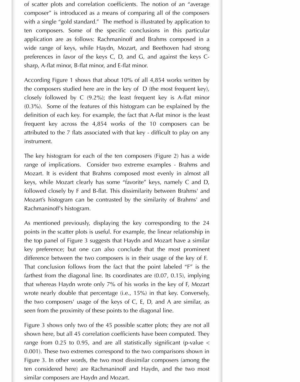
As mentioned previously, displaying the key corresponding to the 24

points in the scatter plots is useful. For example, the linear relationship in

the top panel of Figure 3 suggests that Haydn and Mozart have a similar

key preference; but one can also conclude that the most prominent

difference between the two composers is in their usage of the key of F.

That conclusion follows from the fact that the point labeled “F” is the

farthest from the diagonal line. Its coordinates are (0.07, 0.15), implying

that whereas Haydn wrote only 7% of his works in the key of F, Mozart

wrote nearly double that percentage (i.e., 15%) in that key. Conversely,

the two composers' usage of the keys of C, E, D, and A are similar, as

seen from the proximity of these points to the diagonal line.

Figure 3 shows only two of the 45 possible scatter plots; they are not all

shown here, but all 45 correlation coefficients have been computed. They

range from 0.25 to 0.95, and are all statistically significant (p-value <

0.001). These two extremes correspond to the two comparisons shown in

Figure 3. In other words, the two most dissimilar composers (among the

ten considered here) are Rachmaninoff and Haydn, and the two most

similar composers are Haydn and Mozart.

As shown above, an alternative to pairwise comparisons is to compare

each composer's histogram to the histogram of all works. The

corresponding scatter plots are shown in Figure 4; the corresponding r-

values range from 0.36 to 0.91 (all with p-values < 0.001). Given the

large scatter of points in the top/left panel, it follows that Rachmaninoff’s

key usage is the least similar to the overall key usage (r = 0.36). Said

differently, Rachmaninoff can be considered the most atypical of the ten

composers examined here. By contrast, both Schubert and Tchaikovsky

have a key usage which is very similar to the overall key usage (r = 0.91).

As such, they can be considered the most typical of the ten composers.

The work presented here can be extended in a number of ways. Here,

the key associated with each work is that officially assigned to that work

according to IMSLP. For example, the key associated with Beethoven’s 5th

symphony is C minor, regardless of the key changes within the first

movement, or across the various movements. It will be interesting to

apply the above analysis to each and every key that makes an appearance

anywhere in a work. Other possible extensions would take into account

the musical form (e.g., symphony versus solo-instrument), the choice of

the instrument (e.g., piano versus clarinet), and the musical era to which

the composer belongs.

Finally, one can supplement the above analysis by providing “theoretical”

arguments that may explain the conclusions found here. For example, the

ranking of the composers in Figure 4 begs some explanation. The manner

in which Rachmaninoff emerges as an atypical composer may be

attributed to the fact that he belongs to a different era than the rest of the

composers. However, that explanation is not entirely satisfactory for two

reasons: 1) Brahms, a transition composer between the Classical era and

the Romantic era, is the second-ranking atypical composer, while 2)

Bach, a Baroque composer, emerges as a relatively typical composer (r =

0.86). In other words, the composer’s era appears to be unrelated to the

ranking in Figure 4. In way of a different explanation, one may suspect

the ranking is a consequence of the total number of works written by

each composer. If that were the case, then the number of works

displayed atop each panel in Figure 2 would display some pattern

(increasing or decreasing); but they do not. As such, there appears to be

no simple theoretical explanation for the ranking of the composers in

Figure 4. Another possible explanation may follow from analyzing the

historically established relationships between composers; for example, it

is well-known that Mendelssohn was influenced by Bach10; this may

explain why both composers appear with comparable correlation

coefficients (r=0.86) in Figure 4. It will be important to establish other

©THE JOURNAL OF EXPERIMENTAL SECONDARY SCIENCE, ISSN#2162-8092

such historical connections in order to explain the conclusions found

here.

References

1. Comprehensive musical analysis. Metuchen, N.J.: Scarecrow Press.

White, J. D. 1994.

2. The New Oxford History of Music, Volume I. Oxford University Press.

Wellesz, E. (1957).

3. Medieval music. New York: W.W. Norton. Hoppin, R. H. (1978).

4. Buelow, G. J. (2001). Affects, Theory of the. The New Grove

Dictionary of Music and Musicians, second edition, edited by Stanley

Sadie and John Tyrrell. London: Macmillan Publishers.

5. Beethoven's Piano Sonatas: A Short Companion. New Haven: Yale

University Press. p. 134, Rosen, C. (2002).

6. Nettheim, N. (1999). The Statistics of Schubert's Keys. The

Schubertian, No. 26, 2-3. http://nettheim.com/publications/schuberts-

keys.htm

7. Instrumentation/orchestration. New York: Longman, Blatter, A. (1980).

8. IMSLP/Petrucci Music Library: Free Public Domain Sheet Music. N.p.,

n.d. Web. 20 Aug. 2013. http://imslp.org.

9. Mind on Statistics, Thomson Learning, Inc., Utts, J. M. and Heckard,

R.F. (2007).

10. Mendelssohn: A Life in Music. Oxford Press, Todd, L. (2003).

Acknowledgements

We thank Bahman Shahid-Saless, the director of the Boulder Chamber

Philharmonic, and Richard Karpen, School of Music, University of

Washington, for reading an early version of this article and for providing

useful comments.