on the variance curve of outputs for some queues and networks yoni nazarathy gideon weiss yoav...
TRANSCRIPT

1
On the variance curve of outputs for some queues and
networks
Yoni NazarathyGideon WeissYoav Kerner
QPA Seminar,EURANDOM January 8, 2009

2
Queueing System
Output Counts
t
1( , )D t
3( , )D t 2( , )D t
Var( ( ))D t
t
( )D t
Example 1: Stationary stable M/M/1, D(t) is PoissonProcess:( )
Example 2: Stationary M/M/1/1 with . D(t) is RenewalProcess(Erlang(2, )):
21 1 1
Var( ( ))4 8 8
tD t t e
Var( ( ))D t t
(1)Vt B o
B
V
Asymptotic Variance RateV
B Y-intercept

3
Outline of the Talk: Models and Methods
Outline of the Talk: Models and Methods
Models:• Finite Capacity Birth Death Queues (M/M/1/K)
• General Lossless Queues
• M/G/1 Queue
• Push-Pull (infinite supply) Network
• Infinite supply re-entrant line
Methods:• Markovian Arrival Process (MAP)
• Embedding in Renewal Reward
• Regenerative Simulation (Renewal Reward)
• Diffusion Limits

4
Finite CapacityBirth-Death Queues
5
1*
0
K
ii
V v
2
2 ii i
i
Mv M
d
*
1i i iM D P
1
i
i jj
P
0
i
i jj
D d
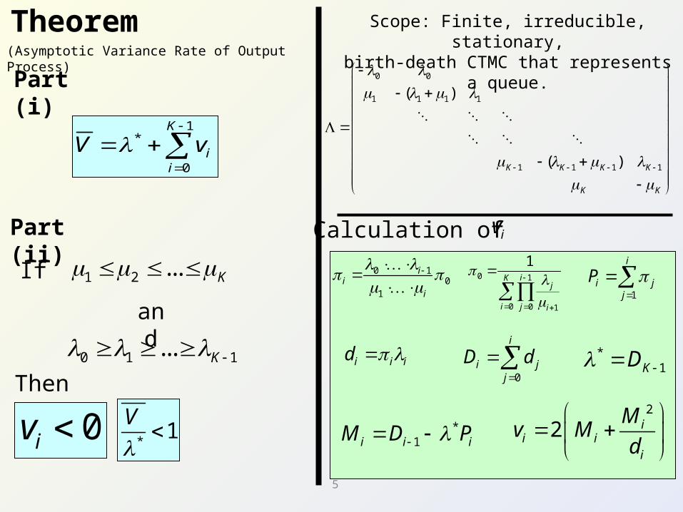
Theorem
i i id
Part (i)
Part (ii)
0iv
1 2 ... K
0 1 1... K
*1
V
0 0
1 1 1 1
1 1 1 1
( )
( )K K K K
K K
*1KD
Scope: Finite, irreducible, stationary,birth-death CTMC that represents a queue.
0 10
1
ii
i
0 1
0 0 1
1iK
j
i j i
and
If
Then
Calculation of iv
(Asymptotic Variance Rate of Output Process)

6
**
V V
BRAVO Effect (M/M/1/K)
2
2
1 2 1
1 3
21
3 6 3
(1 )(1 (1 2 ) (1 ) )1
(1 )
K K K
K
K K
K KV
K
2lim
3KV

7
C D
* * 2 * 2 3 2Var ( ) 2( ) 2 2( ) 2 ( )1 1 r bt
BV
D t D D t D O t e
0 0
1 1 1 1
1 1 1 1
( )
( )K K K K
K K
1
1
0 0
0 0
0
0K
K
* 1D *E[ ( )]D t t
0 0
1 1 1
1 1 1
0 ( )
0 ( )
0K K K
K
Generator Transitions without events Transitions with events
1( )1
, 0r b
Method: Markovian Arrival Process

8
General LosslessQueues
9
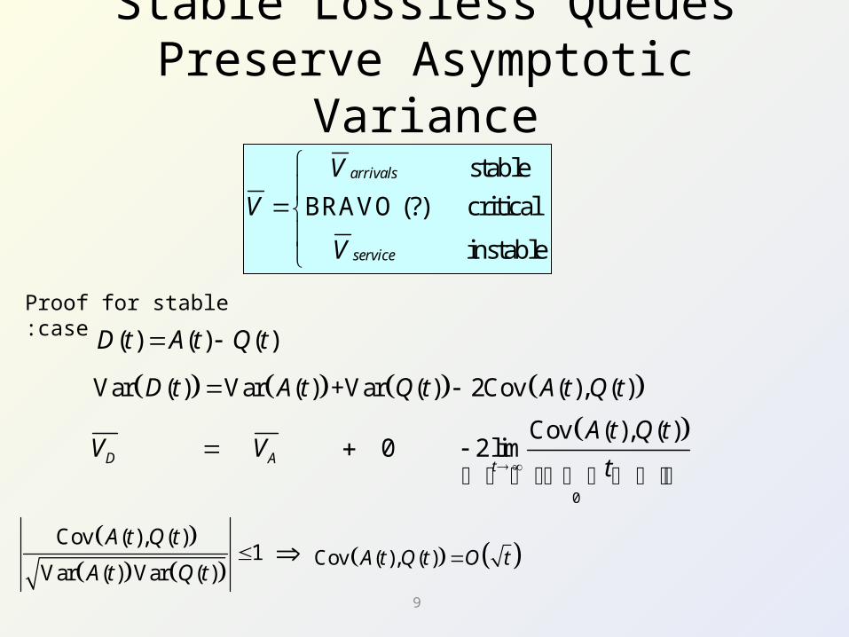
Stable Lossless Queues Preserve Asymptotic Variance
stable
BRAVO (?) critical
instable
arrivals
service
V
V
V
Cov ( ), ( )1
Var ( ) Var ( )
A t Q t
A t Q t Cov ( ), ( )A t Q t O t
( ) ( ) ( )D t A t Q t
0
Var ( ) Var ( ) +Var ( ) 2Cov ( ), ( )
Cov ( ), ( ) 0 2 limD A
t
D t A t Q t A t Q t
A t Q tV V
t
Proof for stable case:

10
M/G/1 Queue

11
M/G/1 Linear AsymptoteTheorem:
4 4 2 4 2 2 2 3 3 2 4 3 3
2
2
3 6 18 18 10 18 4 (1 )Stationary
12(1 )
Starting Empty(1 )
c c c c c
B
( ) (1)Var D t t B o
1, 2 (Exponential like) B 0
1, 2 B 0
1, 2 B 0
c
c
c

12
Shape of Variance Curve (?)
0 B
0 B
0t
Var ( )D t
1, 2 B 0
1, 2 B 0
c
c
Pas Op: Possible non-sense ahead
!!!

13
( )R t
Derivation Method:Embedding in Renewal Reward
( )D t
t
V
V
a
ar
r ( )
( ) (1
(1)
)
R RR t V t
D t V
o
t o
B
B
2
11
1
R
R
R
nV m
m
V
B
V
B
0t
0 0( ) ( )D t R t
Busy Cycle Duration
Number Customers
Served
14
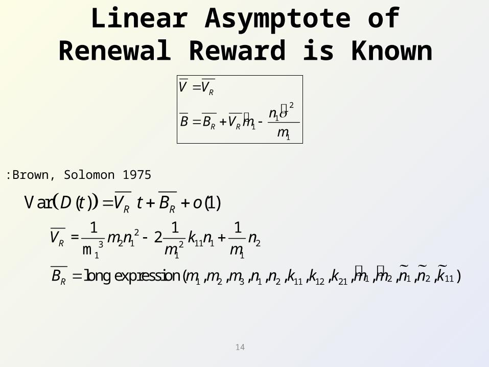
Linear Asymptote of Renewal Reward is Known
Linear Asymptote of Renewal Reward is Known
Var ( ) (1)R RD t V t B o
22 1 11 1 23 2
1 1 1
1 2 1 2 111 2 3 1 2 11 12 21
1 1 1 = 2
m
long expression( , , , , , , , , , , , , )
R
R
V m n k n nm m
B m m m n n k k k m m n n k
Brown, Solomon 1975:
2
11
1
R
R R
V V
nB B V m
m

15
Using in Regenerative Simulation

16
t
1( , )D t
3( , )D t 2( , )D t ( )Var D T
VT
( )D t
( )(1)
Var D T BV o
T T T
Naive Estimation of Asymptotic Variance:
There is bias due to intercept:
Regenerative Estimation of Asymptotic Variance:
22 1 11 1 23 2
1 1 1
1 1 1 = 2
mRV m n k n nm m
Estimate moments of busy cycle and number served…. Plug in…
17
0 .2 0 .4 0 .6 0 .8 1 .0 1 .2
0 .2
0 .4
0 .6
0 .8
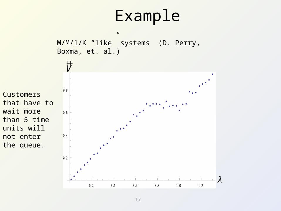
Example
M/M/1/K “like” systems (D. Perry, Boxma, et. al.)
V
Customers that have to wait more than 5 time units will not enter the queue.

18
A Push-Pull Queueing Network
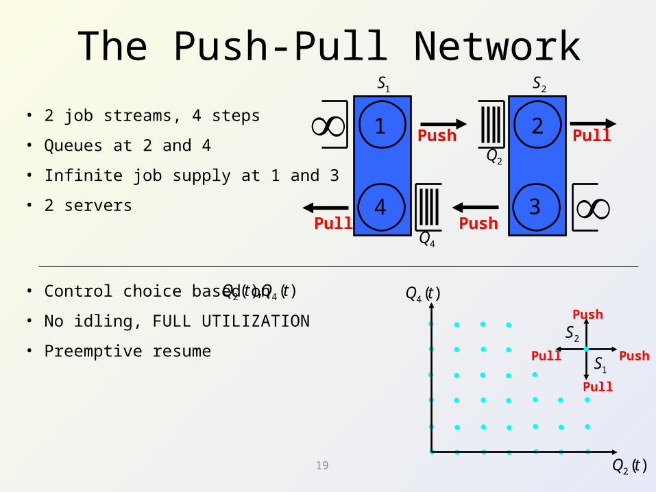
19 2 ( )Q t
4 ( )Q t
1S
2S
• 2 job streams, 4 steps
• Queues at 2 and 4
• Infinite job supply at 1 and 3
• 2 servers
The Push-Pull Network
1 2
34
1S 2S
2 4( ), ( )Q t Q t• Control choice based on
• No idling, FULL UTILIZATION
• Preemptive resume
Push
Push
Pull
Pull
Push
Push
Pull
Pull
2Q
4Q

20
Policies
1 2
4 3
Inherently stable
Inherently unstable
Policy: Pull priority (LBFS)
Policy: Linear thresholds
1 2
4 3
1 2
34
TypicalBehavior:
2 ( )Q t
4 ( )Q t
2,4
1S 2S
3
4
2 1
1,3
TypicalBehavior:
5 0 1 0 0 1 5 0 2 0 0 2 5 0 3 0 0
5
1 0
2 2 4Q Q
4 1 2Q Q
Server: “don’t let opposite queue go below threshold”
1S
2S
Push
Pull
Pull
Push
1,3

21
KSRS
1 2
34

22
M/G/. Pull Priority
M G
MG
2 2 2 2 2 21 11 1 2 1 2 2 1 1 1 2 1 1 2 2 23
1 2 1 2
(1 )( ) ( )( )( )
V c c
Using the Renewal Reward Method :
1
2
1 1,c
2 2,c
Number served of type 1, during a cycle is 0 w.p. . 2
1 2

23
Using DiffusionLimits
Now assume general processing times with finite second moment.

24
Network View of the Model
1
1 4 2 3
k
k
1
Dynamics
( ) sup{ : }
(0) 0, ( )
( ) ( ) , ( ) ( )
D ( ) ( ( ))
(0) 0, Q (t) 0
( ) (0) ( ) ( )
nj
k kj
k k
k k
k
k k k k
S t n t
T T t
T t T t t T t T t t
t S T t
Q
Q t Q D t D t
4 1 2 1
0 0
Pull priority policy
( ) ( ) 0 ( ) ( ) 0t t
Q s dT s Q s dT s 4 1 2 1 2 2 4 3
0 0
2 4 4 4 2 21 20 0
Linear thresholds policy
{0 ( ) ( )} ( ) 0 {0 ( ) ( )} ( ) 0
1 1
{ ( ) ( )} ( ) 0 { ( ) ( )} ( ) 0
1 1
1 1
t t
t t
Q s Q s dT s Q s Q s dT s
Q s Q s dT s Q s Q s dT s
2 4 1 2 3 4
Network process
( ) ( ), ( ), ( ), ( ), ( ), ( )Y t Q t Q t T t T t T t T t
or
1 2
34
1S 2S

25
Stability Result
( ) Q(t), U(t)X t
1 2
34
Queue Residual
is strong Markov with state space
( )X t
Theorem: X(t) is positive Harris recurrent.
Proof follows framework of Jim Dai (1995)
2 Things to Prove:
1. Stability of fluid limit model
2. Compact sets are petite
Positive Harris Recurrence:

26
Diffusion Scaling
Now find a limiting process, such that . ( )D t ( ) ( )wn
nD t D t
Var (1)V D
27
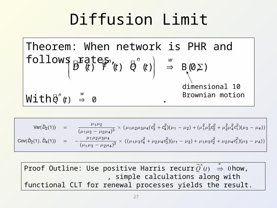
Diffusion Limit
Theorem: When network is PHR and follows rates,
With .
( ) ( ) ( ) B(0, )n wn n
D t T t Q t
10 dimensional Brownian motion
( ) 0wn
Q t
Proof Outline: Use positive Harris recurrence to show, , simple calculations along with functional CLT for renewal processes yields the result.

28
Infinite SupplyRe-entrant Lines

29
Infinite Supply Re-entrant Line
4
2
1C
1 3
56
78
10 9
( )D t
2C 3C
4C
2
13
1
: For any stable policy (e.g. LBFS): .k
k C
mkk C
Thm V
1
1Infinite QueuesSupply
1
1
2 21
1
1 {2,..., } ... ,
1 .
Means: ,...,
Variances: ,...,
1, i=2,...,Ii
I
k
k
kk C
i kk C
K C C
C
m m
m
m

30
“Renewal Like”
4
2
1C
1 3
56
78
10 9
2C 3C
4C1
1
2
3
kk C
kk C
V
m
1C
1
6
8
10
Renewal Output1 1 1 1 2 2 2 2 3 3 3 31 6 8 10 1 6 8 10 1 6 8 10
Job 1 Job 2 Job 3
, , , , , , , , , , , ,....x x x x x x x x x x x x
1 1 1 1 2 2 2 3 3 3 31 6 8 10 6 8 1 1 6 8 10
201, , , , , , , , , , , , ,...x x x x x x x x x x xx

31
Thank You

32
Extensions

33
• Inherently stable network
• Inherently unstable network
• Unbalanced network
• Completely balanced network
Configuration 1 2
34
1 2
4 3
1 2
4 3
1 2 1 2
4 3 4 3
or
1 2
4 3

34
Calculation of Rates
1
2
2 3 41 2 1
1 3 2 4
4 1 23 4 3
1 3 2 4
( )
( )
1 4 3 21 , 1
1 2
4 3
1 1 2 2
4 4 3 3
1 2
34
Corollary: Under assumption (A1), w.p. 1,
every fluid limit satisfies: .
k - Time proportion server works on k
k -Rate of inflow, outflow through k
Full utilization:
Stability:
( ) , ( )k kk kT t t D t t

35
Memoryless Processing(Kopzon et. al.)
1 2
4 3
Inherently stable
Inherently unstable
Policy: Pull priority
Policy: Generalized thresholds
1 2
4 3
1 2
34
1S 2S
Alternating M/M/1 Busy Periods
Results:Explicit steady state:
Stability (Foster – Lyapounov)
- Diagonal thresholds
2 ( )Q t
4 ( )Q t
- Fixed thresholds

36

37

38

39

40

41
Proof Outline
1*
0
K
ii
V v
Whitt: Book: 2001 - Stochastic Process Limits,.
Paper: 1992 - Asymptotic Formulas for Markov Processes…
1) Lemma: Look at M(t) instead of D(t).
2) Proposition: The “Fully Counting” MAP of M(t) has associated MMPP with same variance.
3) Results of Ward Whitt: An explicit expression of asymptotic variance rate of birth-death MMPP.
42
t
3 2 1
2 4 2
1 1 2
a b c
a
b
c
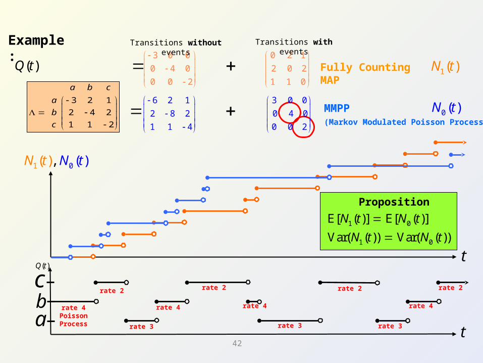
MMPP (Markov Modulated Poisson Process)
Example:
0 ( )N t
tabc
( )Q t
rate 4Poisson Process
rate 2
rate 3
rate 4
rate 2
rate 4
rate 3
rate 2
rate 3
rate 4
rate 2
1 0
1 0
E[ ( )] E[ ( )]
Var( ( )) Var( ( ))
N t N t
N t N t
Proposition
3 0 0 0 2 1
0 4 0 2 0 2
0 0 2 1 1 0
6 2 1 3 0 0
2 8 2 0 4 0
1 1 4 0 0 2
Transitions without events Transitions with events
1( )N tFully Counting MAP
1( ),N t
( )Q t
0 ( )N t

43
0 1 KK – 1
Some intuition for M/M/1/K-BRAVO
…

44
V
c
c
M/M/40/40
M/M/10/10
M/M/1/40
1
K=20K=30
c=30
c=20

45
V
1
MAP used for PH/PH/1/40 with Erlang and Hyper-Exp distributions
1
2

46
The “2/3 property”The “2/3 property”
K
• GI/G/1/K
• SCV of arrival = SCV of service
• 1 V2 42 33
3 21
2 3
6 2 455 3
1 2 132 3

47
,
2 3
,
1
11
lim Corr( ( ), ( )) 15 5 3
4 12 2 4
1
K
t
K
R
KD t L t
K K K
R
1 12
,1 2 1 2 2 1
(1 )(1 3 ) (1 )(3 )
(1 )(1 (2 1)(1 ) )((1 )(1 ) 4( 1)(1 ) )
K K K K
KK K K K K
KR
K
0.139772 1
1lim Corr( ( ), ( )) 1
41
12
tD t L t
For Large K
( )D t
( )L t
48
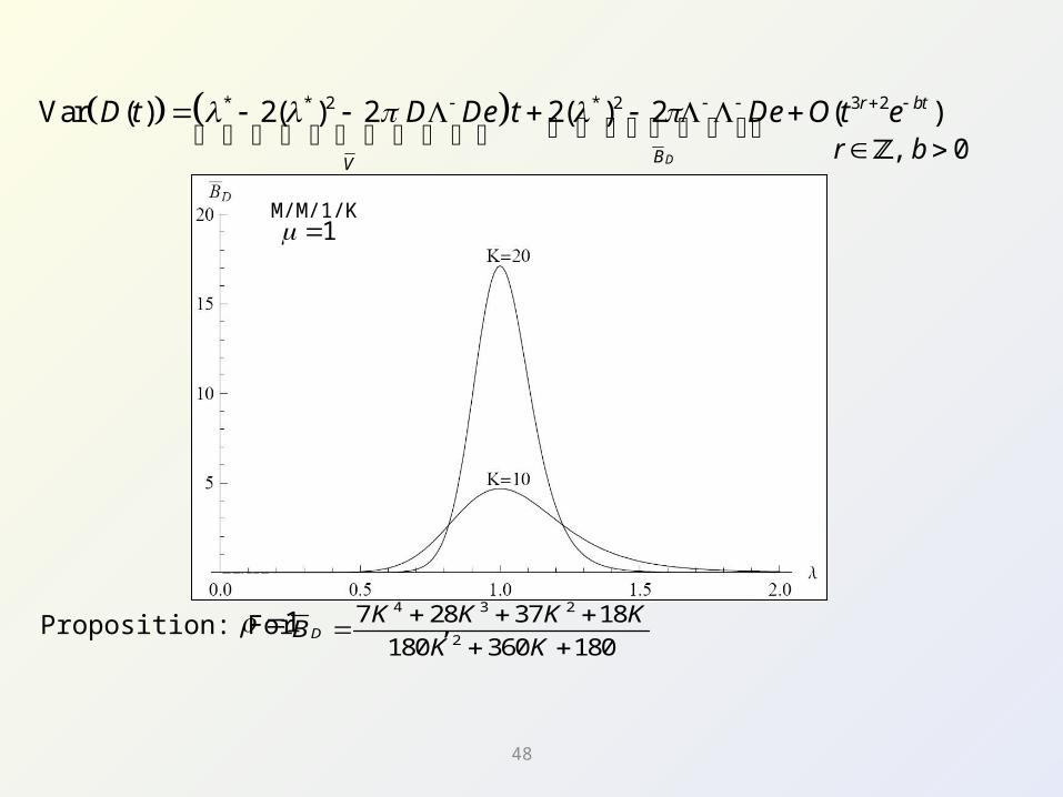
Proposition: For ,4 3 2
2
7 28 37 18
180 360 180D
K K K KB
K K
M/M/1/K1
* * 2 * 2 3 2Var ( ) 2( ) 2 2( ) 2 ( )
D
r bt
BV
D t D De t De O t e , 0r b
1