on the well-posedness of a mathematical model of quorum
TRANSCRIPT

On the Well-Posedness of a Mathematical Model ofQuorum-Sensing in Patchy Biofilm Communities
Stefanie Sonner1, Messoud A Efendiev1,∗, Hermann J Eberl2
1 Institute for Biomathematics and Biometry,Helmholtz Center Munich, Neuherberg, Germany
2 Department of Mathematics and Statistics,University of Guelph, Guelph, On, Canada
∗ corresponding author
April 15, 2011
AbstractWe analyze a system of reaction-diffusion equations that models quorum-
sensing in a growing biofilm. The model comprises two nonlinear diffusion effects:a porous medium type degeneracy, and super diffusion. We prove the well-posedness of the model. In particular, we present for the first time a uniquenessresult for this type of problem. Moreover, we illustrate the behavior of modelsolutions in numerical simulations.
MSC2010: 35K65, 35K57, 92C17, 92D25
1 Introduction
Most bacteria live in biofilm communities rather than in planktonic cultures. Biofilmsare bacterial accumulations forming on biotic or abiotic surfaces (called substrata)in aqueous surroundings. Whenever the environmental conditions allow for bacterialgrowth, cells attach to the substratum and start to grow and divide. They produce agel-like layer, the so-called EPS (extracellular polymeric substances) [13]. Embeddedin the self-produced EPS biofilm bacteria are better protected against harmful envi-ronmental impacts than planktonic bacteria. For example, cells in biofilm colonies aremore resistant against antibiotic agents, and the EPS protects them against mechanicalwash-out [13].
Biofilms are important in applications in various fields. They are beneficially usedin environmental engineering technologies, e.g. for groundwater protection and wastew-ater treatment. However, in other occurrences biofilms can be harmful. If they form
1

on implants and natural surfaces in the human body, they can provoke bacterial infec-tions. Biofilm contamination can lead to health risks in food processing environments,and biofouling of industrial equipment or ships can cause severe economic defects forthe industry.
Quorum-sensing is a cell-cell communication mechanism used by bacteria to coordi-nate gene expression and behavior in groups based on the local density of the bacterialpopulation [12]. Bacteria constantly produce and release low amounts of signalingmolecules (also called autoinducers). When the concentration of autoinducers passesa certain threshold, the cells are rapidly induced, and switch from a so-called down-regulated to an up-regulated state. In an up-regulated state they typically produce thesignaling molecule at a highly increased rate.
Quorum sensing is not yet very well-understood. Different biological theories andinterpretations exist [12], which are currently actively researched, both in experimentalmicrobiology and in mathematical and theoretical biology, primarily for planktonicbacterial populations but also in the context of biofilms. In this paper we are concernedwith analytical aspects of the biofilm growth and quorum sensing model introduced in[10].
Mathematical models of biofilms have been studied for several decades. They rangefrom traditional one-dimensional models that describe biofilms as homogeneous layers,to more recent two- and three-dimensional biofilm models that account for the spa-tial heterogeneity of biofilm communities that can be observed in the lab. For thelatter a variety of mathematical modeling concepts has been suggested, including dis-crete stochastic particle based models, discrete stochastic cellular automata, and de-terministic continuum models based on the description of the mechanical properties ofbiofilms [23]. The model that we study is based on an interpretation of a biofilm asa continuous, spatially structured microbial population. It is a system of four highlynonlinear reaction-diffusion equations for the dependent variables volume fractions ofup-regulated and down-regulated cells, concentration of a growth limiting nutrient andconcentration of the signaling molecule. The model was originally proposed in [10],where in numerical simulations the contribution of environmental hydrodynamics tothe transport of signaling molecules and its effect on inter-colony communication andup-regulation was studied. Analytical aspects of the model were not addressed; forexample the question of well-posedness was left open. This will be studied in ourarticle.
The quorum-sensing model extends the single-species biofilm growth model that wasoriginally proposed in [6]. It is combined with a model for quorum-sensing in planktoniccultures that was suggested in [16]. The prototype biofilm model [6] consists of tworeaction-diffusion equations for the biomass density and the growth limiting substrate.The diffusion coefficient for biomass vanishes for vanishing biomass density and itblows up if the biomass density approaches an upper bound. Thus, the model containstwo nonlinear diffusion effects. It degenerates like the porous medium equation andit shows super diffusion. This prototype model was mathematically analyzed andnumerically studied in a series of papers, for both mathematical and biological interest(cf. [3, 5, 7, 9]). In particular, an existence and uniqueness result could be established.
The prototype single-species single-substrate biofilm model has been previously
2
extended to model biofilms which consist of several types of biomass and accountfor multiple dissolved substrates. The model introduced in [2] describes the diffusiveresistance of biofilms against the penetration by antibiotics. In [19] an amensalis-tic biofilm control system was modeled (a beneficial biofilm controls the growth of apathogenic biofilm). In both articles, existence proofs for the solutions were given,and numerical studies were presented. The structure of the governing equations of thementioned multi-species models is similar, however, differs essentially from the mono-species model. Therefore, the analytical results for the prototype model could not allbe carried over to the more involved dual-species case. For example, the question ofuniqueness of solutions remained unanswered in [2] and [19].
Compared to the models in [2, 19], the particularity of the quorum sensing modelis, that adding the governing equations for the two biomass fractions, i.e. for the up-and down-regulated cells, we recover exactly the mono-species biofilm model. Takingadvantage of the results obtained in [9] for the single-species model we are able toprove the existence and uniqueness of solutions of the quorum-sensing model and thecontinuous dependence of solutions on initial data. We want to emphasize that it is thefirst time a uniqueness result is obtained for multi-species diffusion-reaction models ofbiofilms that extend the prototype model [6]. Our proof of the existence of solutions isbased on the non-degenerate approximations developed in [9]. However, our approachin the present paper is different and leads to a uniqueness result for the solutions. Wehope that this will help us to answer the question of uniqueness of solutions for theantibiotic and probiotic model, which was left open in the articles [2] and [19].
2 Mathematical Model
A mathematical description of quorum-sensing in biofilms requires to distinguish twotypes of bacteria, the up-regulated cells and the down-regulated cells, and to include amechanism by which cells switch between these two states.
We are concerned with the model of quorum sensing in biofilm communities pro-posed in [10], which extends the mono-species biofilm growth model [6] and combinesit with a mathematical model of quorum-sensing for suspended populations [18]. Thedependent model variables are the volume fraction occupied by the down-regulated andup-regulated cells, the concentration of the signaling molecule, and the concentrationof the growth-limiting nutrient. The EPS is implicitly taken into account, in the sensethat biomass volume fractions describe the sum of biomass and EPS assuming thattheir volume ratio is constant. Since the number of cells that can be accommodatedper unit volume is limited by a given constant, the volume fraction occupied by biomasscan also be understood as a measure for biomass density.
The model is formulated in terms of a system of nonlinear reaction-diffusion equa-tions in a bounded spatial domain Ω ⊂ Rn, n ∈ 1, 2, 3. The spatial independentvariable is denoted by x ∈ Ω and t ≥ 0 denotes the time variable. The dependentvariables X and Y denote the volume fractions occupied by down- and up-regulatedbiomass, respectively. The dependent variables A and S denote the concentrations ofthe autoinducer and of the growth controlling substrate. Both are assumed to be dis-
3

solved and do not occupy space. In dimensionless form, these four dependent variablessatisfy the parabolic system
∂tX = dO · (DM(M)OX) + k3XS
k2+S− k4X − k5A
mX + k5Y
∂tY = dO · (DM(M)OY ) + k3Y S
k2+S− k4Y + k5A
mX − k5Y
∂tS = O · (DS(M)OS)− k1SM
k2+S
∂tA = O · (DA(M)OA)− γA + αX + (α + β)Y.
(1)
The constants d, k2 and γ are positive, m ≥ 1 and the coefficients k1, k3, k4, k5, α andβ are non-negative. The total biomass fraction M = X + Y denotes the volumefraction occupied by up-regulated or down-regulated cells. The biomass componentsare normalized with respect to the physically maximal possible cell density, hence wenecessarily require M = X + Y ≤ 1. The autoinducer concentration A is normalizedwith respect to the threshold concentration for induction. Thus, induction occurslocally in the biofilm if A reaches approximately 1 from below. If A locally decreasesfrom a value larger than 1 to a value below 1, down-regulation at constant rate k5
will dominate. Finally, the substrate concentration S is normalized with respect to acharacteristic value for the system, such as the nutrient concentration at the boundaryof the domain, if Dirichlet conditions are applied.
The solid region occupied by the biofilm as well as the liquid area are assumedto be continua. The actual biofilm is then described by the region Ω2(t) := x ∈Ω | M(x, t) > 0 and the liquid surroundings by Ω1(t) := x ∈ Ω | M(x, t) = 0. Thesubstratum, on which the biofilm grows, is part of the boundary ∂Ω.
In our model, induction switches the cells between down- and up-regulated states,without changing their growth behavior. This includes, for example, microbial systemsin which induction affects only virulence factors, or the composition of EPS but nottheir production rates. Under this hypothesis we can assume that the spatial spreadingof both biomass fractions is described by the same diffusion operator
DM(M) :=Ma
(1−M)b
with a, b ≥ 1. The biomass motility constant d > 0 in the equations for the biomasscomponents is small compared to the diffusion coefficients DS and DA of the dissolvedsubstrates. This reflects that the cells are to some extent immobilized in the EPSmatrix. Spatial expansion of the biofilm is driven by biomass accumulation. Thebiomass diffusion coefficient DM(M) vanishes when the total biomass approaches zeroand blows up when the biomass density tends to its maximum value. The polynomialdegeneracy Ma is well-known from the porous medium equation, it guarantees thatspatial spreading is negligible for low values of M and yields the separation of biofilmand liquid phase, i.e. a finite speed of interface propagation. Spreading of biomassonly takes place when the total biomass fraction takes values close to its maximalpossible value. For M = 1 instantaneous spreading occurs, known as the effect ofsuper diffusion. The singularity at M = 1 ensures the maximal bound for the biomassdensity, which is a physical limitation as the number of cells that fits into a unit volumeis bounded. Since biomass is produced as long as sufficient nutrients are available, this
4

upper bound cannot be guaranteed by the growth terms alone. The degeneracy Ma
alone does not yield this maximum bound for the cell density, while the singularity (1−M)−b does not guarantee the separation of biofilm and liquid region by a sharp interface.Consequently, both nonlinear diffusion effects together are required to describe spatialexpansion of the biofilm.
The diffusion coefficients of the dissolved substrates depend on the cell densityas well, however in a non-critical way. The diffusion coefficients DS and DA are lowerinside the biofilm than in the surrounding liquid region. In [10] the linearization ansatz
DS,A(M) = DS,A(0)−M(DS,A(0)−DS,A(1)
),
is made, where DS,A(0) denotes the diffusion coefficient in water and and DS,A(1)the diffusion coefficient in a fully compressed biofilm. Hence, the functions DS(M)and DA(M) are bounded from below and above by a positive constant and essentiallybehave like Fickian diffusion. In fact, in many cases, in particular for substrates ofsmall molecule size, such as oxygen, carbon, etc., DS,A(0) ≈ DS,A(1). Without loss ofgenerality in the sequel we assume
DS(M) = d1
DA(M) = d2,
where the constants d1 and d2 are positive.Apart from the spatial spreading of biomass and the diffusive transport of signaling
molecules and nutrients the following processes are included in the model:
• Up-regulated and down-regulated biomass is produced due to the consumptionof nutrients. This mechanism is described by Monod reaction terms, where theconstant k3 reflects the maximum specific growth rate, and k2 the Monod halfsaturation constant. The constant k1 is the maximum specific consumption rate,which can be computed from the maximum growth rate and a yield coefficientthat indicates how much substrate is required to produce a unit of biomass.Generally, k1 À k3 holds. For our non-dimensional formulation we choose thetime-scale for growth, i.e. 1/k3, for normalization. Thus, k3 = 1.
• Natural cell death is included and described by the lysis rate k4. This effect canbe dominant compared to cell growth, if the substrate concentration becomessufficiently small.
• The signaling molecules decay abiotically at rate γ.
• Due to an increase of the autoinducer concentration A down-regulated cells areconverted into up-regulated cells at rate κ5A
m. Modeling this by mass actionkinetics we obtain for the degree of polymerization m in the synthesis of thesignaling molecule, m = 2. We lump additional secondary processes into thisconstant and obtain a value 2 < m < 3 [10]. Up-regulated cells are convertedback to down-regulated cells at constant rate κ5. If A < 1 the latter effectdominates, if A > 1 up-regulation is super-linear.
5
• Finally, down-regulated cells produce the signaling molecule at rate α, while up-regulated cells produce it at the increased rate α + β, where β is one order ofmagnitude larger than α. For technical reasons, we will require in our analysisα + β > γ, i.e. the signaling molecule production rate of the up-regulated cells ishigher than the abiotic decay rate. For all practical purposes, this is not a severemodel restriction; see also Table 4.1, where a set of parameters is compiled fromthe literature. If the opposite was true, the autoinducer molecules would decayfaster than they are produced in an up-regulated system and no noteworthyaccumulation could take place.
It remains to specify initial and boundary values for the biomass fractions andsubstrate concentrations to complete the model (2), which will be made more precisein the following section.
3 Analysis
3.1 Preliminaries
We study, for technical reasons, the model in the auxiliary form
∂tX = dO · (DM(M)OX) + k3XS
k2+S− k4X − k5|A|mX + k5|Y |
∂tY = dO · (DM(M)OY ) + k3Y S
k2+S− k4Y + k5|A|mX − k5|Y |
∂tS = d1∆S − k1SM
k2+S
∂tA = d2∆A− γA + αX + (α + β)Y.
(2)
but point out that non-negative solutions of (1) solve (2) and vice versa, i.e. afternon-negativity is shown |.| can be removed from the first and second equation of (2) toobtain (1).
For simplicity we assume homogeneous Dirichlet boundary conditions for the biomasscomponents X and Y and the concentration of the signaling molecule A, and constantDirichlet conditions for the nutrient concentration S
X|∂Ω = Y |∂Ω = A|∂Ω = 0
S|∂Ω = 1.(3)
If the biofilm is contained in the inner region of Ω, away from its boundary, thissituation describes a growing biofilm in the absence of a substratum. Such biofilms areoften called microbial flocs, which play a major role in biological wastewater treatment.The boundary conditions imposed on the concentration of nutrients reflect a constantunlimited nutrient supply at the boundary of the considered domain. Similarly, keepingA = 0 at the boundary, enforces a removal of autoinducers from the domain. Theseare very specific boundary conditions, primarily chosen for convenience. However, thesolution theory we develop in the following sections easily carries over to more generalboundary values, which are relevant and often more appropriate for applications.
6

The initial data for the model variables are given by
X|t=0 = X0, Y |t=0 = Y0, S|t=0 = S0, A|t=0 = A0 (4)
with S0, X0, Y0, A0 ∈ L2(Ω) satisfying the compatibility conditions and
0 ≤ S0(x) ≤ 1, 0 ≤ A0(x) ≤ 1
X0(x) ≥ 0, Y0(x) ≥ 0, X0(x) + Y0(x) ≤ 1(5)
for almost every x ∈ Ω. In fact, usually, the initial autoinducer concentration A0 ≡ 0.For T > 0 we denote the parabolic cylinder by QT := Ω×]0, T ].
Definition 3.1. We call the vector valued function (X, Y, A, S) a solution of system(2) with boundary and initial data (3) and (4), if its components belong to the class
X, Y,A, S ∈ C([0, T ]; L2(Ω)) ∩ L∞(QT )
A, S ∈ L2((0, T ); H1(Ω))
DM(M)OX, DM(M)OY ∈ L2((0, T ); L2(Ω))
for any T > 0 and satisfy system (2) in distributional sense.
To be more precise, if (X, Y, A, S) is a solution according to Definition 3.1, thenthe equality∫
Ω
X(x, T )ϕ(x)dx−∫
Ω
X0(x)ϕ(x)dx = −d
∫
QT
DM(M(x, t))OX(x, t) · Oϕ(x)dtdx
+
∫
QT
(k3
X(x, t)S(x, t)
k2 + S(x, t)− k4X(x, t)− k5|A(x, t)|mX(x, t) + k5|Y (x, t)|
)ϕ(x)dtdx
holds for all test-functions ϕ ∈ C∞c (Ω) and almost every T > 0. The determining
equations for the other components of the solution are defined in an analogous way.Compared to other biofilm models with several particulate substances, such as
[2, 19], the particularity of the quorum-sensing model (2) is that we recover the single-species biofilm growth model for the total biomass fraction M and the nutrient concen-tration S. Indeed, adding the equations for the biomass fractions X and Y in system(2) we obtain
∂tM = dO · (DM(M)OM) + k3
MSk2+S
− k4M
∂tS = d1∆S − k1SM
k2+S
(6)
with initial and boundary values
M |∂Ω = 0, S|∂Ω = 1
M |t=0 = M0 = X0 + Y0, S|t=0 = S0,
which is exactly the single species biofilm-model proposed in [6]. A solution theory forthis system was developed in [9]. Our proof of the well-posedness of the quorum-sensingmodel will be essentially based on the results obtained for the mono-species model. Forthe convenience of the reader we recall and summarize all relevant properties of thesolutions of system (6), which will be used in the sequel. The following theorem yieldsexistence and regularity results for the solutions.
7
Theorem 3.2. If the initial data satisfy
S0 ∈ L∞(Ω) ∩H1(Ω)
0 ≤ S0(x) ≤ 1, S0|∂Ω = 1
M0 ∈ L∞(Ω), F (M0) ∈ H10 (Ω)
M0 ≥ 0, ‖M0‖L∞(Ω) < 1,
(7)
where F (M) :=∫ M
0za
(1−z)b dz, 0 ≤ M < 1, then there exists a unique solution (M, S)
satisfying (6) in the sense of distributions and the solution belongs to the class
M,S ∈ L∞(Ω× R+) ∩ C(R+; L2(Ω))
F (M), S ∈ L∞(R+; H1(Ω)) ∩ C(R+; L2(Ω))
0 ≤ S(x, t),M(x, t) ≤ 1, ‖M‖L∞(Ω×R+) < 1.
(8)
Furthermore, the following estimates hold
‖S(t)‖2H1(Ω) + ‖F (M(t))‖2
H1(Ω) ≤ C(‖S0‖2H1(Ω) + ‖F (M0)‖2
H1(Ω) + 1)
‖S(t)‖2H1(Ω) + ‖∂tS(t)‖2
H−1(Ω) + ‖F (M(t))‖2H1(Ω)
+ ‖M(t)‖2Hs(Ω) + ‖∂tM(t)‖2
H−1(Ω) ≤ C(1 +1
tκ),
for some constant C ≥ 0, where 0 < s < 1b+1
and κ ≥ 1. The constants are independentof the initial data (S0,M0).
For further details and the proof see Theorem 3.1 in [9]. Moreover, the semigroupgenerated by the solutions of system (6) is Lipschitz-continuous in L1(Ω)-norm. Thefollowing result recalls Theorem 3.2 of [9].
Proposition 3.3. Let (S,M) and (S, M) be two solutions of system (6) corresponding
to initial data (S0,M0), respectively (S0, M0), and the initial data satisfy the assump-tions of the previous theorem. Then, the following estimate holds
‖S(t)− S(t)‖L1(Ω) + ‖M(t)− M(t)‖L1(Ω)
≤ e(k1+k2+k3)t(‖S0 − S0‖L1(Ω) + ‖M0 − M0‖L1(Ω)
).
In particular, the solution is unique within class (8).
Another important result for our analysis is that the biomass density does notattain the singularity as long as the initial concentration does not take this value (cf.Proposition 3.3 in [3]).
Proposition 3.4. If the initial data (S0,M0) satisfy the assumptions of Theorem 3.2and there exists some δ ∈ (0, 1) such that
‖M0‖L∞(Ω) = 1− δ,
then the corresponding solution (S, M) satisfies
‖M(t)‖L∞(Ω) ≤ 1− η
for t > 0 and some η ∈ (0, 1), where the constant η depends on δ and Ω only.
8

Consequently, the substrate concentration S and the total biomass density M canbe regarded as known functions and the original system (2) reduces to a system ofequations for the biomass fraction X and the concentration of the quorum-sensingsignaling molecule A
∂tX = dO · (DOX) + k3XS
k2 + S− k4X − k5|A|mX + k5(M −X)
∂tA = d2∆A− γA + αX + (α + β)(M −X),
where the diffusion coefficient of the biomass fraction is defined by D(x, t) := (M(x,t))a
(1−M(x,t))b .
Here, we used the positivity of the biomass component Y , which will be proved in Sec-tion 3.3. We rewrite this non-autonomous semi-linear system with bounded coefficientsas
∂tX = dO · (DOX) + gX − k5|A|mX + h
∂tA = d2∆A− γA− βX + l,(9)
where the interaction terms are given by the known functions
g(x, t) := k3S(x, t)
k2 + S(x, t)− k4 − k5
h(x, t) := k5M(x, t) ≥ 0
l(x, t) := (α + β)M(x, t) ≥ 0.
Note that all coefficient functions are bounded, g, h, l ∈ L∞(Ω×R+) by Theorem 3.2,and the diffusion coefficient D is non-negative and bounded by Theorem 3.3. Indeed,if the initial density satisfies 0 ≤ M0 < 1 − δ for some δ ∈ (0, 1), then there exists apositive constant η ∈ (0, 1) such that 0 ≤ M(x, t) ≤ 1 − η for almost all t > 0 andx ∈ Ω. Consequently,
0 ≤ D(x, t) =(M(x, t))a
(1−M(x, t))b≤ 1
(1−M(x, t))b≤ 1
ηb,
that is, D is non-negative and satisfies D ∈ L∞(Ω× R+).The solution theory can be extended to less regular initial data and other boundary
conditions. Moreover, it was shown in [9] that the semi-group generated by the solutionsof system (6) is continuous in L1(Ω)-norm and possesses a compact global attractor.
3.2 Uniqueness
In this paragraph we prove the uniqueness and L2(Ω)-Lipschitz-continuity of solutionswith respect to initial data of the semi-linear parabolic system (9) with bounded co-efficients, which degenerates when the total biomass density M approaches zero. Weconsider initial data X0, Y0, A0 ∈ H1
0 (Ω), S0 ∈ H1(Ω) such that S0|∂Ω = 1 and
0 ≤ S0, X0, Y0, A0 ≤ 1, ‖X0 + Y0‖L∞(Ω) < 1.
9

Theorem 3.5. We assume that the initial data (X0, Y0, S0, A0) satisfy the assumptionsstated above. Then, there exists at most one non-negative solution (X,A) of system(9) within the class of solutions considered in Definition 3.1.
Proof. We assume (X, A) and (X, A) are two such solutions corresponding to initial
data (X0, A0) and define their differences u := X−X and v := A− A. Then, v belongsto the space L2((0, T ); H1
0 (Ω)), u satisfies DM(M(t))Ou(t) ∈ L2(Ω) for almost everyt ∈ (0, T ] and ∂tu, ∂tv ∈ L2((0, T ); H−1(Ω)) for some T > 0. Moreover, the functions uand v satisfy the system
∂tu = dO · (DOu) + gu− k5(A
mX − AmX)
∂tv = d2∆v − γv − βu
with zero initial and boundary conditions
v|t=0 = u|t=0 = 0
u|∂Ω = v|∂Ω = 0.
If we formally multiply the second equation by v and integrate over Ω, we obtain theestimate
1
2
d
dt‖v(·, t)‖2
L2(Ω) = −d2‖Ov(·, t)‖2L2(Ω) − γ‖v(·, t)‖2
L2(Ω) − β⟨u(·, t)v(·, t)⟩
L2(Ω)
≤ −γ‖v(·, t)‖2L2(Ω) − β
⟨u(·, t)v(·, t)⟩
L2(Ω)
where we used the positivity of d2. Multiplying the first equation by u and integratingover Ω yields
1
2
d
dt‖u(·, t)‖L2(Ω) = −d
∫
Ω
D(x, t)|Ou(x, t)|2dx +
∫
Ω
g(x, t)|u(x, t)|2dx
−k5
∫
Ω
[Am(x, t)X(x, t)− Am(x, t)X(x, t)]u(x, t)dx.
In order to estimate the last integral we observe
AmX − AmX = Amu + X(Am − Am) = Amu + vXm
∫ 1
0
(sA + (1− s)A)m−1ds.
Since D, A and X are non-negative we obtain
1
2
d
dt‖u(·, t)‖L2(Ω) ≤
∫
Ω
g(x, t)|u(t, x)|2dx + k5
∫
Ω
Am(x, t)u2(x, t)dx
+ k5
∫
Ω
X(x, t)v(x, t)u(x, t)m
∫ 1
0
(sA(x, t) + (1− s)A(x, t))m−1dsdx
≤ C1‖u(·, t)‖L2(Ω) + C2
⟨u(·, t)v(·, t)⟩
L2(Ω),
10

for some constants C1, C2 ≥ 0. Here, we used that the functions A, A, X and g belong tothe class L∞(QT ). Adding both inequalities and using the Cauchy-Schwarz inequalityyields
d
dt
(‖u(., t)‖2L2(Ω) + ‖v(., t)‖2
L2(Ω)
) ≤ C3
(‖u(., t)‖2L2(Ω) + ‖v(., t)‖2
L2(Ω)
), (10)
for some C3 ≥ 0. Invoking Gronwall’s Lemma and the initial conditions u|t=0 = v|t=0 =0, it follows u = v = 0 almost everywhere.
For the definiteness of the integrals appearing in the estimates of our proof we referto the next paragraph.
Note that the proof of Theorem 3.5 implies the Lipschitz-continuity in L2(Ω)-normof the semigroup generated by the solutions of the initial-/boundary-value problem (9).
Corollary 3.6. Let (X, A) and (X, A) be two solutions of system (9) within the class
of the previous theorem corresponding to initial data (X0, A0), respectively (X0, A0).Then, the following estimate holds
‖X(·, t)− X(·, t)‖2L2(Ω) + ‖A(·, t)− A(·, t)‖2
L2(Ω)
≤ eCt(‖X0 − X0‖2
L2(Ω) + ‖A0 − A0‖2L2(Ω)
),
for some constant C ≥ 0.
Proof. The estimate follows immediately from inequality (10) in the proof of Theorem3.5 and Gronwall’s Lemma.
Hence, assuming existence and uniqueness of solutions, the semi-group generatedby the solutions of system (9) is Lipschitz-continuous in the topology of L2(Ω)×L2(Ω)
‖(X(t)− X(t), A(t)− A(t))‖L2(Ω)×L2(Ω) ≤ eCt‖(X(0)− X(0), A(0)− A(0)
)‖L2(Ω)×L2(Ω).
As we pointed out in the preliminary paragraph of this section the question ofuniqueness of solutions of the original system (2) reduces to prove the uniquenessof solutions of the semi-linear system (9). We formally obtained the uniqueness ofsolutions of the quorum-sensing model, the existence of solutions within the statedclass will be shown in the following paragraph.
3.3 Existence
In order to prove the existence of solutions of the original system we consider non-degenerate auxiliary systems and show that the solutions of the auxiliary systemsconverge to the solution of the degenerate problem when the regularization parametertends to zero. The ideas are based on the method developed in [9] for the mono-speciesmodel and the strategy applied in [2] and [19] to prove the existence of solutions of
11
multi-species biofilm models. For small ε > 0 we define the non-degenerate approxi-mation of system (2) by
∂tX = dO · (Dε,M(M)OX) + k3XS
k2+S− k4X − k5|A|mX + k5|Y |
∂tY = dO · (Dε,M(M)OY ) + k3Y S
k2+S− k4Y + k5|A|mX − k5|Y |
∂tS = d1∆S − k1SM
k2+S
∂tA = d2∆A− γA + αX + (α + β)Y,
(11)
where the regularized diffusion coefficient is defined as
Dε,M(z) :=
(z+ε)a
(1−z)b z ≤ 1− ε1εb z ≥ 1− ε.
Furthermore, we assume the initial data is regular and smooth, namely, that it belongsto the class
S0 ∈ L∞(Ω) ∩H1(Ω), 0 ≤ S0(x) ≤ 1, S0|∂Ω = 1
A0 ∈ L∞(Ω) ∩H10 (Ω), 0 ≤ A0(x) ≤ 1
M0 = X0 + Y0 ∈ L∞(Ω), X0, Y0, F (M0) ∈ H10 (Ω)
X0, Y0 ≥ 0, ‖M0‖L∞(Ω) < 1,
(12)
where F (M) :=∫ M
0za
(1−z)b dz, for 0 ≤ M < 1.
Adding the equations for the biomass components X and Y of system (11) werecover the non-degenerate auxiliary system for the single-species model
∂tM = dO · (Dε,M(M)OM) + k3MS
k2+S− k4M
∂tS = d1∆S − k1SM
k2+S,
(13)
which is a regularized version of (6). In [9] it was shown that for every (sufficientlysmall) ε > 0 there exists a unique solution (Sε,Mε) of system (13) and the solutionsare uniformly bounded with respect to the regularization parameter ε. Moreover, ifthe initial data belongs to class (12), the solution Mε is separated from the singularity.To be more precise, there exists a constant η ∈ (0, 1), which is independent of ε, suchthat Mε(x, t) < 1− η holds for all x ∈ Ω, t > 0 (cf. Proposition 6 in [9]).
Hence, we may regard Mε = Xε + Yε and Sε as known functions and the problemreduces to prove the existence of solutions of the semi-linear system
∂tX = dO · (DεOX) + gεX − k5|A|mX + hε
∂tA = d2∆A− γA− βX + lε
X|∂Ω = 0, A|∂Ω = 0
X|t=0 = X0, A|t=0 = A0.
(14)
The diffusion coefficient is defined as Dε(x, t) := Dε,M(Mε(x, t)) and the interactionfunctions are given by
gε(x, t) := k3Sε(x, t)
k2 + Sε(x, t)− k4 − k5
hε(x, t) := k5Mε(x, t) ≥ 0
lε(x, t) := (α + β)Mε(x, t) ≥ 0,
12

where (Mε, Sε) denotes the solution of the non-degenerate approximation (13). Here,we already used the positivity of the biomass component Yε, which will be proved inthe following lemma. In order to abbreviate the notation we introduce the new reactionterms f ε
1 and f ε2,
f ε1(x, t,X(x, t), A(x, t)) := gε(x, t)X(x, t)− k5|A(x, t)|mX(x, t) + hε(x, t)
f ε2(x, t,X(x, t), A(x, t)) := −γA(x, t)− βX(x, t) + lε(x, t).
We first show that all components of the solution of the non-degenerate approxi-mation are non-negative and bounded.
Lemma 3.7. The components of the solution (Xε, Yε, Sε, Aε) of the auxiliary system(11) are non-negative and belong to the class L∞(Ω× R+).
Proof. The substrate concentration Sε and the total biomass density Mε = Xε +Yε arenon-negative and bounded by 1 according to Proposition 6 in [9]. We will show thatthe components Xε, Yε and Aε are non-negative. As Xε +Yε = Mε ≤ 1 this immediatelyimplies the boundedness of the biomass fractions Xε and Yε. The boundedness of themolecule concentration Aε then follows by a comparison theorem for scalar parabolicequations (cf. [22]). Indeed, the constant Amax := α+β
γ> 1 is a supersolution for Aε.
It satisfies Amax|∂Ω ≥ 0 = Aε|∂Ω, Amax|t=0 ≥ A0 = Aε|t=0 and
∂tAmax − d2∆Amax + γAmax − αXε − (α + β)Yε
= γAmax − αXε − (α + β)Yε ≥ γAmax − α− β = 0,
where we used that α + β > γ (cf. Section 2). It remains to prove the positivityof the components Xε, Yε and Aε. To this end we again apply a comparison theoremfor parabolic equations to the biomass fraction of down-regulated cells: The constantX = 0 is a subsolution for Xε. Indeed, it satisfies Xε|∂Ω ≥ 0 = X|∂Ω, X0 = Xε|t=0 ≥0 = X|t=0 and
∂tX − dO · (Dε,M(Mε)OX)− k3XSε
k2 + Sε
+ k4X + k5|Aε|mX − k5|Yε| = −k5|Yε| ≤ 0.
By the same arguments and owing to the positivity of Xε, the constant solution Y = 0is also a subsolution for Yε, so we conclude Yε ≥ 0. Finally follows Aε ≥ 0, by comparingwith the subsolution A = 0 for the biomass fraction Aε and using the fact that thecomponents Xε and Yε are non-negative.
Having established positivity and uniform boundedness of solutions we are in aposition to prove the existence of solutions of the reduced system (14). To this end wetreat the region where the total biomass density becomes small and its complementin QT := Ω×]0, T ] separately. In [9] it was shown that the solution (S,M) of thesingle-species model is obtained via the L2(Ω)-limit of the solutions (Sε,Mε) of thenon-degenerate approximations
S(t) = limε→0
Sε(t), M(t) = limε→0
Mε(t)
13

in C([0, T ]; L2(Ω)), where T > 0 is arbitrary. We now define the domains
Qδ,T := (x, t) ∈ QT | M(t, x) < δand Qc
δ,T := QT \Qδ,T for some δ ∈ (0, 1). Note that both subsets are open due to theHolder-continuity of the solution M (cf. [2]).
Lemma 3.8. We assume the initial data belongs to class (12). Then, for all sufficientlysmall ε > 0 there exists a unique solution (Aε, Xε) of the auxiliary system (14) satisfying
Xε, Aε ∈ L2((0, T ); H10 (Ω)) ∩ C([0, T ]; L2(Ω)) ∩ L∞(QT )
∂tXε, ∂tAε ∈ L2((0, T ); H−1(Ω)).
Moreover, the solutions are uniformly bounded with respect to ε and satisfy the estimates
maxt∈[0,T ]
‖Xε(·, t)‖L2(Ω) + ‖Xε‖L2((0,T );H10 (Ω)) + ‖∂tXε‖L2((0,T );H−1(Ω) ≤ Cε
4
(1 + ‖X0‖L2(Ω)
)
maxt∈[0,T ]
‖Aε(·, t)‖L2(Ω) + ‖Aε‖L2((0,T );H10 (Ω)) + ‖∂tAε‖L2((0,T );H−1(Ω)) ≤ C5(1 + ‖A0‖L2(Ω)),
for some constants Cε4, C5 ≥ 0, where C5 is independent of ε. The solutions are even
Holder-continuousXε ∈ Cαε,
αε2 (QT ), Aε ∈ Cα, α
2 (QT )
for some αε, α > 0. The Holder constant αε depends on the parameter ε, the data anduniform bound of the approximate solutions only, the constant α is independent of ε.
Finally, restricted to the domain Qcδ,T the solutions Xε satisfy all estimates uni-
formly. To be more precise, the constant Cε4 in the inequality above and the Holder
constant αε are independent of ε > 0 for the family of approximate solutions Xε,where Xε := Xε|Qc
δ,T.
Proof. If the initial data M0 and S0 belong to class (12) the total biomass density Mε
satisfies Mε(t, x) < 1− η in QT for some η ∈ (0, 1), and the constant η is independentof ε. This implies that the diffusion coefficient Dε is positive and uniformly boundedfrom above by a constant independent of ε. Indeed, for all ε < η
εa ≤ Dε(Mε(x, t)) =(Mε(x, t) + ε)a
(1−Mε(x, t))b≤ (1− η + ε)a
(1− (1− η))b≤ 1
ηb
holds, that is Dε ∈ L∞(QT ) and strictly positive. Hence, for all sufficiently smallε > 0 the semi-linear auxiliary system (14) is regular and uniformly parabolic. Thefunctions gε, hε, lε, Aε and Xε are uniformly bounded with respect to the regularizationparameter ε by Lemma 3.7, which implies that the interaction functions f ε
1 and f ε2 are
uniformly bounded in QT . By standard arguments (Galerkin approximations) followthe existence and uniqueness of the approximate solution (Xε, Aε) belonging to theclass stated in the lemma and satisfying the given estimates (cf. [21]). Moreover, theHolder-continuity of solutions follows from Theorem 10.1, Chapter III in [20].
Note that due to the uniform boundedness of the approximate solutions the com-ponent Aε satisfies the semi-linear equation
∂tAε − d2∆Aε = Hε,
14

where the function Hε is uniformly bounded, ‖Hε‖L∞(QT ) ≤ c, for some constant cindependent of ε > 0. Hence, the constants in the estimates for the component Aε canbe chosen independently of ε.
Finally, if ε > 0 is sufficiently small, then Mε ≥ δ2
holds in the region Qcδ,T . Hence,
the diffusion coefficient restricted to the domain Qcδ,T is uniformly bounded from above
and below by a positive constant, which is independent of ε > 0
(δ
2
)a
≤ (δ
2+ ε)a ≤ Dε(Mε(x, t)) =
(Mε(x, t) + ε)a
(1−Mε(x, t))b≤ 1
ηb.
It is a well-known fact for non-degenerate parabolic equations of second order withcoefficients in L∞(Ω), that the solution is bounded in terms of the coefficients of theequation (cf. [20]), which concludes the proof of the lemma.
In the sequel, we will use this lemma to pass to the limit in the region Qcδ,T . To
pass to the limit in the region Qδ,T further requires uniform estimates for the family ofapproximate solutions.
Lemma 3.9. If ε > 0 is sufficiently small, the product√DεOXε is uniformly bounded
in L2(QT ) and the approximate solutions satisfy Xε(t) ∈ Hs(Ω) for some s > 0 andalmost every t > 0. Moreover, there exists ε0 > 0 such that for all ε < ε0
‖Xε‖L2((0,T );Hs(Ω)) ≤ C
holds, where the constant C ≥ 0 is independent of ε.
Proof. Multiplying the first equation of system (14) by Xε and integrating over Ω weobtain
1
2
d
dt‖Xε(·, t)‖2
L2(Ω) + d
∫
Ω
Dε(x, t)|OXε(x, t)|2dx
=
∫
Ω
Xε(x, t)f ε1 (x, t, Xε(x, t), Aε(x, t)) dx ≤ C6,
for some constant C6 ≥ 0. Due to Lemma 3.7 the constant C6 is independent of ε. Byintegrating this inequality from 0 to T > 0 follows the first statement of the lemma.
Furthermore, for sufficiently small ε > 0 we obtain Xε ≤ Mε ≤ 1 − η and conse-quently
Xaε ≤ Dε,M(Xε) =
(Xε + ε)a
(1−Xε)b≤ (Xε + Yε + ε)a
(1− (Xε + Yε))b= Dε,M(Mε)
holds. So we derive the estimate∫
Ω
Xaε (x, t)|OXε(x, t)|2dx ≤
∫
Ω
Dε,M(Mε(x, t))|OXε(x, t)|2dx ≤ C7,
for some constant C7 ≥ 0 independent of the regularization parameter ε > 0. This
shows that Xa2ε (t)|OXε(t)| ∈ L2(Ω) or equivalently, X
a2+1
ε (t) ∈ H1(Ω) for almost everyt ∈]0, T ]. Finally, if a function satisfies ϕβ ∈ H1(Ω) for some β > 1, then ϕ ∈ W s,2β(Ω)
15

holds for all s ≤ 1β. This implies Xε(t) ∈ W s,2(a
2+1)(Ω) for s ≤ 1
a2+1
. Since the
domain Ω is bounded and a ≥ 1 the embedding W s,2a(Ω) → Hs(Ω) is continuous andwe deduce Xε(t) ∈ Hs(Ω) for some positive s > 0. In particular, this proves thatthe family of approximate solutions Xε is uniformly bounded in the Hilbert spaceL2((0, T ); Hs(Ω)).
Lemma 3.10. There exist functions
X∗ ∈ L∞(QT ) ∩ L2((0, T ); Hs(Ω))
A∗ ∈ L∞(QT ) ∩ L2((0, T ); H10 (Ω))
and a sequence (εk)k∈N tending to zero for k →∞ such that the family of solutions ofthe auxiliary systems (14) converge weakly
Xεk X∗, Aεk
A∗
in L2((0, T ); Hs(Ω)), respectively L2((0, T ); H10 (Ω)), and strongly
Xεk→ X∗, Aεk
→ A∗
in C([0, T ]; L2(Ω)) when k tends to infinity.
Proof. We will prove the convergence and existence of the limit for the biomass fractionX∗, the arguments are similar for the molecule concentration A∗. By Lemma 3.9for sufficiently small ε > 0 the family of approximate solutions Xεε>0 is uniformlybounded in the Hilbert space L2((0, T ); Hs(Ω)) for some s > 0. Hence, there existsan element X∗ ∈ L2((0, T ); Hs(Ω)) and a sequence (εk)k∈N tending to zero for k →∞such that the sequence (Xεk
)k∈N converges weakly to X∗ in L2((0, T ); Hs(Ω)).Furthermore, due to Lemma 3.9 the product
√DεOXε is uniformly bounded inL2(QT ) and the diffusion coefficient satisfies Dε ∈ L∞(QT ). Consequently, we obtain
‖Dε|OXε|‖2L2(QT ) ≤ ‖Dε‖L∞(QT )‖
√Dε|OXε|‖2
L2(QT ) ≤ c,
for some constant c ≥ 0 independent of ε, which implies the uniform boundedness of∂tXε in L2((0, T ); H−1(Ω)).
By Theorem 1.5, Chapter II in [1] now follows the strong convergence of the sequenceof approximate solutions in C([0, T ]; L2(Ω)).
It remains to show that the limits of the approximate solutions yield the solutionof the degenerate problem.
Theorem 3.11. The limits X∗ and A∗ of the solutions of the non-degenerate approx-imations are the unique weak solutions of the reduced system (9). In particular, thereexists a unique solution of the quorum-sensing model (2).
Proof. We show that we can pass to the limit ε → 0 in the distributional formulation ofthe non-degenerate auxiliary system (14). We will only prove the convergence for thebiomass fraction X∗ as the arguments are the same or even simplify for the molecule
16

concentration A∗. The functions Xε are weak solutions of the auxiliary systems (14),that is
∫
Ω
Xε(x, T )ϕ(x)dx−∫
Ω
X0(x)ϕ(x)dx
= −d
∫
QT
Dε(x, t)OXε(x, t) · Oϕ(x)dtdx +
∫
QT
f ε1(x, t, Aε(x, t), Xε(x, t))ϕ(x)dtdx
holds for all test-functions ϕ ∈ C∞c (Ω) and almost every T > 0. As the family of
approximate solutions is uniformly bounded in L∞(QT ) by Lemma 3.7, passing to thelimit in the integrals is immediate, except for the diffusion term. Hence, it remains toshow the convergence of the term
∫
QT
Dε(x, t)OXε(x, t) · Oϕ(x)dtdx =
∫
QT
Dε,M(Mε(x, t))OXε(x, t) · Oϕ(x)dtdx
→∫
QT
DM(M(x, t))OX(x, t) · Oϕ(x)dtdx,
when the regularization parameter ε tends to zero. Note that the integrals are well-defined due to Lemma 3.9. We split the difference and treat the domains Qδ,T and Qc
δ,T
separately. To this end we define
Rε := Iε + Jε :=
∫
Qδ,T
(Dε(x, t)OXε(x, t)−DM(M(x, t))OX(x, t)) · Oϕ(x)dtdx
+
∫
Qcδ,T
(Dε(x, t)OXε(x, t)−DM(M(x, t))OX(x, t)) · Oϕ(x)dtdx,
which does not depend on the parameter δ > 0, and show that the term Rε vanisheswhen ε tends to zero. To estimate the integral Jε we express the difference in thefollowing way
DεOXε −DM(M)OX = (Dε,M(Mε)−DM(M)) OXε + DM(M) (OXε − OX) .
For the first term of the integral we obtain
⟨(Dε,M(Mε)−DM(M))OXε,Oϕ
⟩L2(Qc
δ,T )
≤∥∥Dε,M(Mε)−DM(M)
∥∥L∞(Qc
δ,T )|⟨OXε,Oϕ
⟩L2(Qc
δ,T )|
≤∥∥Dε,M(Mε)−DM(M)
∥∥L∞(Qc
δ,T )
∥∥|Oϕ|∥∥
L2(Qcδ,T )
∥∥|OXε|∥∥
L2(Qcδ,T )
≤ C8
∥∥Dε,M(Mε)−DM(M)∥∥
L∞(Qcδ,T )
for some constant C8 ≥ 0. Here, we used the Cauchy-Schwarz inequality and theuniform boundedness of the family of approximate solutions Xε, when restricted tothe domain Qc
δ,T in the norm induced by L2((0, T ); H10 (Ω)) (cf. Lemma 3.8). The family
of solutions Mε of the non-degenerate approximations of the single-species model isuniformly bounded in the Holder space C α, α
2 (QT ) for some α > 0 (cf. [2]), which implies
17
strong convergence in C(QT ). Furthermore, the solutions of the auxiliary systemssatisfy the uniform estimate Mε ≤ 1− η and consequently, also M ≤ 1− η holds. Onthe interval [0, 1− η] the truncated function Dε,M : [0, 1− η] → R converges uniformlyto DM when ε tends to zero. Splitting further the remaining term
‖Dε,M(Mε)−DM(M)‖L∞(Qcδ,T )
≤ ‖Dε,M(Mε)−Dε,M(M)‖L∞(Qcδ,T ) + ‖Dε,M(M)−DM(M)‖L∞(Qc
δ,T )
we, therefore, note that it vanishes when ε tends to zero.Finally, the convergence of the second integral of Jε
⟨DM(M) (OXε − OX∗) ,Oϕ
⟩L2(Qc
δ,T )
is an immediate consequence of Lemma 3.8. Indeed, restricted to the domain Qcδ,T
the family of approximate solutions is uniformly bounded in the norm induced byL2((0, T ); H1
0 (Ω)), which implies weak convergence in this space. Since the diffusioncoefficient DM(M) belongs to L∞(QT ) by Proposition 3.4, the product DM(M)Oϕdefines an element in the dual space and it follows the convergence of the integral.Summarizing the above estimates we conclude that there exists an ε0 > 0, which isindependent of δ, such that the term Jε becomes arbitrarily small for all ε < ε0.
It remains to estimate the integral Iε. Recall that the domain Qδ,T was defined asthe subset of QT where M < δ. As Mε converges strongly to M in C(QT ) there existsε1 > 0 such that Mε(x, t) < 2δ holds on Qδ,T for all ε < ε1. If ε > 0 is sufficiently smallit therefore follows
Dε(x, t) = Dε,M(Mε(x, t)) =(Mε(x, t) + ε)a
(1−Mε(x, t))b≤ (3δ)a
(1− 2δ)b
for all (x, t) ∈ Qδ,T .Furthermore, the product
√Dε|OXε| is uniformly bounded in L2(QT ) by Lemma3.9, which allows us to use Holder’s inequality to estimate the integral
∫
Qδ,T
Dε(x, t)OXε(x, t) · Oϕ(x)dtdx ≤∥∥√
Dε|OXε|∥∥
L2(QT )
∥∥√Dε|Oϕ|
∥∥L2(Qδ,T )
≤ C9
(∫
Qδ,T
Dε(x, t)|Oϕ(x)|2dtdx
) 12
≤ C9(3δ)
a2
(1− 2δ)b2
‖ϕ‖2L2((0,T );H1(Ω))
where the constant C9 ≥ 0. Estimating the second integral of Iε in the same way weobtain
Iε ≤∫
Qδ,T
∣∣Dε(x, t)OXε(x, t) · Oϕ(x)∣∣dtdx
+
∫
Qδ,T
∣∣DM(M(x, t))OX(x, t) · Oϕ(x)∣∣dtdx ≤ C10
(3δ)a2
(1− 2δ)b2
,
for some constant C10 ≥ 0.
18
To conclude the proof of the theorem let µ > 0 be arbitrary. We first choose δ > 0and a corresponding ε1 > 0 such that
Iε <µ
2
for all ε < ε1. According to the first part of the proof there exists ε0 > 0, which doesnot dependent on δ > 0 such that
Jε <µ
2
for all ε < ε0. Consequently, we obtain
Rε = Iε + Jε < µ
for all ε < minε0, ε1.This proves the existence of a solution (X,A) of the reduced system (9), the unique-
ness of the solution follows by Theorem 3.5. The existence and uniqueness of solutionsof the original system (2) now follows from the existence and uniqueness of the solution(S, M) of the single species model.
Similar as in the article [9], our proof of the well-posedness of the quorum sensingmodel can be extended to less regular initial data and more general boundary conditionsfor the solutions. The boundary conditions for the dissolved substrates S and A, whichdescribe mechanisms of substrate replenishment and autoinducer removal are therebyrather uncritical. For the biomass volume fractions X and Y the results carry over aslong as the values remain below the threshold singularity. This is the case if X +Y < 1is specified somewhere on the boundary. Note, that due to the finite speed of interfacepropagation the biomass boundary conditions in fact are not always and everywhereactive.
4 Two-dimensional Numerical Simulations
Although we could establish the well-posedness of the biofilm quorum sensing model,we are currently not able to describe the solutions of the model qualitatively based onrigorous analytical arguments. Therefore, we will study them in computer simulations.
4.1 Computational preliminaries
For the numerical integration of the model we use a Mickens-type non-local (in time)discretization of the nonlinear diffusion operator and a standard Finite Difference basedFinite Volume method for the spatial discretization on a regular grid. This semi-implicitmethod was first described in [5] for the class of density-dependent diffusion-reactionsystems arising in mono-species biofilm models and then extended to multi-speciessystems in [14, 15]. In every time step it requires the solution of four sparse linearsystems, one for each dependent variable, for which the stabilized biconjugated gradientmethod is used. The algorithm is implemented in Fortran 95, and the computingintensive tasks to determine the nonlinear reaction terms and to solve the linear systems
19

Table 1: Dimensionless model parameters used in this study, adapted from [10], afterchanging the induction threshold and the bulk substrate concentration.parameter symbol valuesubstrate consumption rate k1 794Monod half saturation concentration k2 0.2maximum biomass growth rate k3 1cell lysis rate k4 0.0667up-regulation rate k5 52.7polymerisation exponent m 2.5AHL production rate of down-regulated cells α 92increased AHL production activity by up-regulated cells β 920abiotic AHL decay rate γ 0.02218diffusion coefficient of substrate d1 16.7diffusion coefficient of autoinducer d2 12.9biomass motility coefficient d 1.7 · 10−7
biofilm interface exponent a 4biofilm threshold exponent b 4mass transfer boundary layer thickness λ 1.5system length scale L 1
are parallelized in OpenMP. The simulations presented here are run on a SGI ALTIX350, using up to 6 Itanium-II processors per computation job.
The biological and physical parameter values used in our simulations are summa-rized in Table 4.1. These are the same values that have been used previously in [10],with the exception of the induction threshold parameter τ , which was reduced from70 nM to 10 nM as discussed in [11], and the bulk substrate concentration, which hasbeen reduced by a factor 5. Both parameters are used in the non-dimensionalization.Therefore, these two modifications result in a change of the quantitative values of sev-eral dimensionless parameters used in our simulations, compared to [10]. The systemmodeled by these parameter values corresponds to a Pseudomonas putida biofilm, thegrowth of which is controlled by carbon as the limiting substrate S. The signalingmolecules are Acyl Homoserine Lactones (AHL).
In addition to the visualization of the spatial structure of the biofilms we will alsoplot the total amount of biomass fractions and autoinducers relative to the size of thedomain
Xtotal(t) =1
|Ω|∫
Ω
X(t, x)dx, Ytotal(t) =1
|Ω|∫
Ω
Y (t, x)dx,
and
Atotal(t) =1
|Ω|∫
Ω
A(t, x)dx.
20

4.2 Microbial flocs
In the first simulation we consider a quadratic domain of size L × L, discretized by200× 200 grid cells.
The initial conditions are chosen such that at t = 0 down-regulated biomass isonly located in a heterogeneous region Ω2(0) in the center of the domain. Initially,no up-regulated biomass and no AHL is assumed to be in the system. At t = 0 thesubstrate concentration in the interior is everywhere at the same level as the boundaryconcentration, i.e.
A0 = Y0 = 0, S0 = 1 in Ω,
X0 > 0 in Ω2(0), X0 = 0 in Ω1(0).
The boundary conditions used in this simulation are the Dirichlet boundary conditions(3). This situation describes a heterogeneous microbial floc in the middle of the domain,which will grow as a consequence of substrate supply.
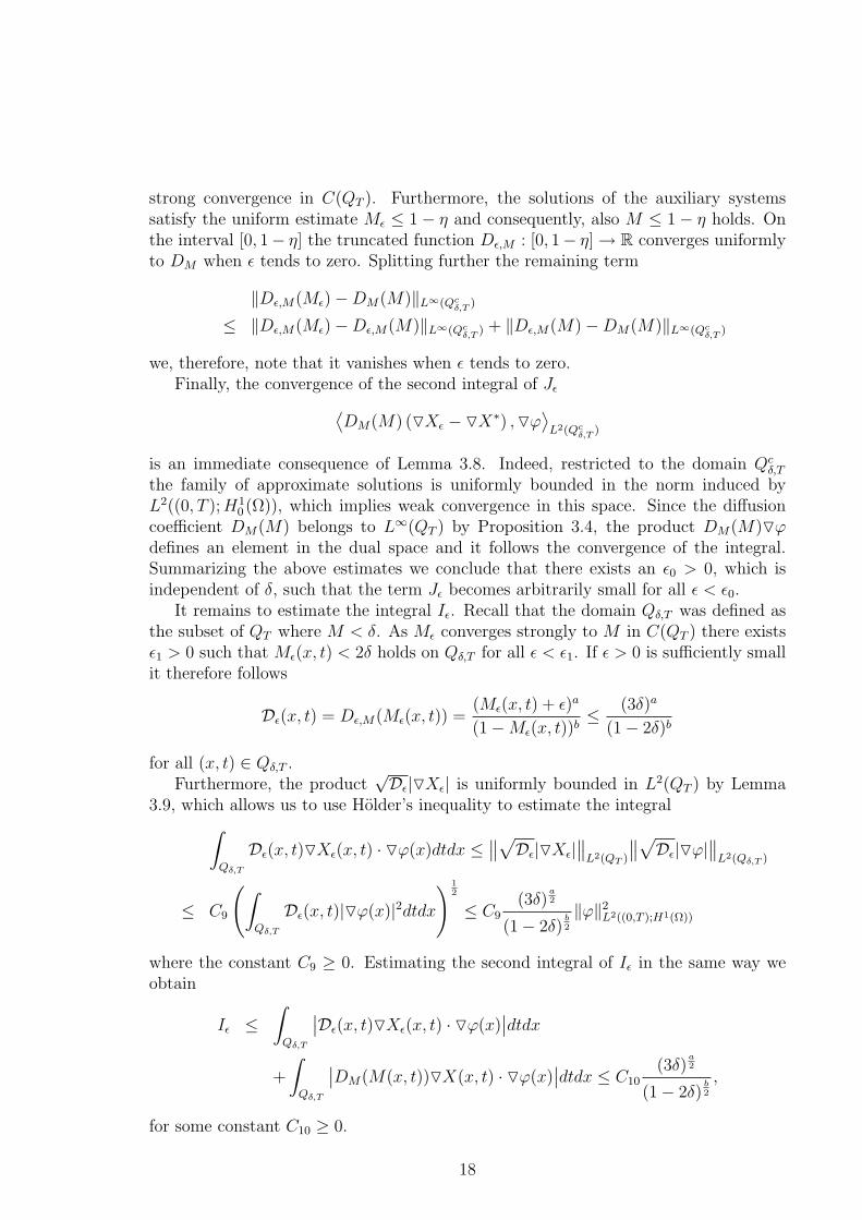
The development and up-regulation of the floc under Dirichlet conditions is shown inFigure 1. The biofilm is represented by the ratio of down-regulated to overall biomass,Z = X/(X + Y ) in the biofilm region Ω2(t), while Z = 0 in the aqueous phase Ω1(t).Moreover, we plot iso-concentration lines for the autoinducer A, coded in greyscale.
Initially the floc is formed by three overlapping circles, which start growing andeventually expand spatially, when the biomass density reaches 1. At t = 1, this origi-nally heterogeneous shape of the floc is still visible, the entire floc is down-regulated.Substrate S is not strongly growth limiting and the floc expands. Here, and in allsubsequent time-steps, the highest AHL concentrations are found in the center of thefloc, from where they diffuse toward the boundary of the domain where the AHL con-centration is kept at A = 0. At t = 2.5 the floc is still entirely down-regulated, but itsshape becomes homogeneous and almost spherical. This is the analogy of the microbialfloc to biofilms which have been found to grow in compact homogeneous layers whensubstrates are not severely limited. At t = 4.0 in the inner core of the floc, a smallamount of up-regulated cells is observed (max Z <= 0.98, i.e. up to 2% of the biomasslocally are upregulated), while at t = 4.3 we note the onset of major up-regulation.At first the biomass in the inner regions undergoes switching, where the AHL con-centration is highest. At t = 4.8 and t = 6.5 the floc is everywhere dominated byup-regulated biomass, although the up-regulation gradient from the center of the flocto the interface is clearly observable. The highest fractions of down-regulated cells canbe found in the outer-most layers.
The lumped quantities Xtotal, Ytotal and Atotal are plotted in the left panel of Figure2. The switch from a down- to an up-regulated system happens instantaneously, att ≈ 4.2. After this switching time the biofilm develops at an unchanged rate, althoughnow dominated by up-regulated cells.
We compare the situation of homogeneous Dirichlet conditions for AHL with asimulation where we pose homogeneous Neumann conditions for the autoinducer in-stead, cf. the right panel of Figure 2. This models the case where autoinducers cannotleave the domain and, therefore, accumulate faster. Consequently, the onset of quorumsensing occurs much sooner under Neumann conditions than under Dirichlet conditions
21
(a) t = 1.0 (b) t = 2.5
(c) t = 4.0 (d) t = 4.3
(e) t = 4.8 (f) t = 6.5
Figure 1: Development and up-regulation of a microbial floc under homogeneous Dirich-let conditions for AHL. Shown are for different t the fraction of down-regulated biomass,Z := X/(X + Y ) (colored), and isolines of the AHL concentration.
22

0
0.1
0.2
0.3
0.4
0.5
0.6
0.7
0 1 2 3 4 5 6 7 8 9 0
0.5
1
1.5
2
2.5
3
3.5
4
biom
ass
AH
L
t
XYA
0
0.005
0.01
0.015
0.02
0.025
0.03
0.035
0 0.2 0.4 0.6 0.8 1 1.2 1.4 0
2
4
6
8
10
12
14
16
X, Y A
t
XYA
Figure 2: Comparison of a quorum sensing simulation of a microbial floc under differentboundary conditions for AHL: Plotted are Xtotal, Ytotal and Atotal for homogeneousDirichlet conditions (left) and for homogeneous Neumann conditions (right) for theautoinducer A.
(t ≈ 0.5 vs. t ≈ 4). This reflects the physical interpretation of the boundary conditionsgiven above: removal of AHL from the system leads to a delay in up-regulation, i.e.not only the number of cells in the system affects up-regulation but also external masstransfer, in this case removal of autoinducers from the system. In the case of Neumannconditions, as a consequence of unhindered accumulation of AHL in the system, veryhigh autoinducer concentrations are reached. Soon after induction occurs, all biomassin the system is up-regulated. At t = 1.2 less than 0.1 % of the entire biomass isstill down-regulated (this condition was implemented as one stopping criterion for thesimulation).
On the other hand, in the case of homogeneous Dirichlet conditions for AHL, muchmore biomass is produced before the onset of up-regulation, while autoinducers accumu-late slower. Up-regulation occurs almost instantaneously, the down-regulated biomassdrops to a small fraction and remains low. At t ≈ 7, we observe a slow increase,which is a boundary effect: The domain Ω2(t) expands and the amount of biomass inthe system increases. The biofilm/water interface comes close to the boundary of thedomain. The expanding and growing of biomass in the system leads to lower substrateconcentrations and higher AHL concentrations in the system. In conjunction with theDirichlet conditions for A and S this has two consequences: The flux of A out of thesystem across the boundary of the domain increases, and so does the flux of substrateinto the system. This slows down up-regulation in the outer layers of the flocs andpromotes growth of down-regulated biomass. As seen in Figure 1, the largest concen-trations of down-regulated cells can be found in the outer layers of the floc. As the flocexpands, the outer layer of the almost spherical floc grows bigger.
4.3 Biofilms
As a second example we simulate quorum sensing in a growing biofilm community thatconsists of several bacterial colonies. The domain Ω is rectangular of size Ω = L×H,
23

discretized by 400 × 200 grid cells. The substratum is randomly inoculated by foursmall pockets of down-regulated biomass, where the biomass density in these pocketsis chosen randomly between two given values, 0.2 ≤ X ≤ 0.4.
The bottom boundary is the substratum which is impermeable to biomass, substrateand AHL. This is described by homogeneous Neumann boundary conditions. Also atthe lateral boundaries homogeneous Neumann conditions are posed for all dependentvariables. These can be understood as symmetry boundary conditions and permit tointerpret our domain as one half of a continuously repeating segment of an infinitedomain.
The top boundary requires a different treatment. This is the boundary throughwhich growth limiting substrate S is added to the system and autoinducer AHL re-moved. Assuming that the bulk liquid at a height λ above the computational domain iscompletely mixed at bulk concentration S = 1 and with molecule concentration A = 0,this is described by the Robin boundary conditions
S + λ∂nS = 1, A + λ∂nA = 0,
on the top boundary, where ∂n denotes, as usual, the outer normal derivative. The newparameter λ resembles the concentration boundary layer thickness of traditional one-dimensional biofilm models, see also [4]. Under this analogy, large values λ correspondto small removal rates of AHL and supply rates of substrate, and vice versa. In one-dimensional biofilm models, this parameter is frequently used to qualitatively mimickthe effect of bulk flow hydrodynamics on mass transfer into and out of the biofilm.Small values of λ correspond to fast bulk flow, large values to slow bulk flow. However,only recently a quantitative relationship between bulk flow velocity and the parameter λwas found for one application [17]. The Robin boundary conditions can be understoodas a combination or interpolation of the two boundary conditions used in the previoussection. Compared to the homogeneous Dirichlet conditions, they correspond to aslower replenishment of nutrients and removal of autoinducers [4].
For both biomass fractions we pose homogeneous Dirichlet conditions at the topboundary. However, since the simulations will always terminate before the biofilmreaches the top boundary, these are, due to the finite speed of interface propagation,in fact, without relevance.
An alternative interpretation of these boundary conditions is a biofilm growing in asmall rectangular crack of depth H + λ in the wall of a much larger completely mixedvessel. In this case, the lateral boundaries can be considered substratum as well.
The initial conditions are chosen as follows: Down-regulated biomass is placed onlyin small pockets at the bottom boundary, i.e. on the substratum, at an inital biomassdensity of X0 < 1, while in the biggest part Ω1(0) of the domain X0 = 0. Depending onthe simulation conducted, these pockets can be located randomly or their location canbe a priori prescribed. The substrate concentration S0 ≡ 1 takes the bulk concentrationvalue everywhere. Initially, no up-regulated cells and no AHL are in the system, i.e.
A0 = Y0 = 0, S0 = 1 in Ω,
X0 > 0 in Ω2(0), X0 = 0 in Ω1(0).
24
After the simulation starts, the biomass starts growing. First, this leads to a con-solidation inside the original biomass pockets, where biomass M increases withoutnoteable spatial expansion. Expansion starts locally when and where the biomass den-sity M approaches 1. Eventually, neighboring colonies merge with neighboring colonies.As long as substrate S is not severely limited the total biomass density M ≈ 1 in thebiofilm. This growth behavior of biofilms according to the underlying diffusion-reactionmodel has been described in much detail previously, e.g. in [6, 7] and is not repeatedhere. Instead we focus on the onset of quorum-sensing activity.
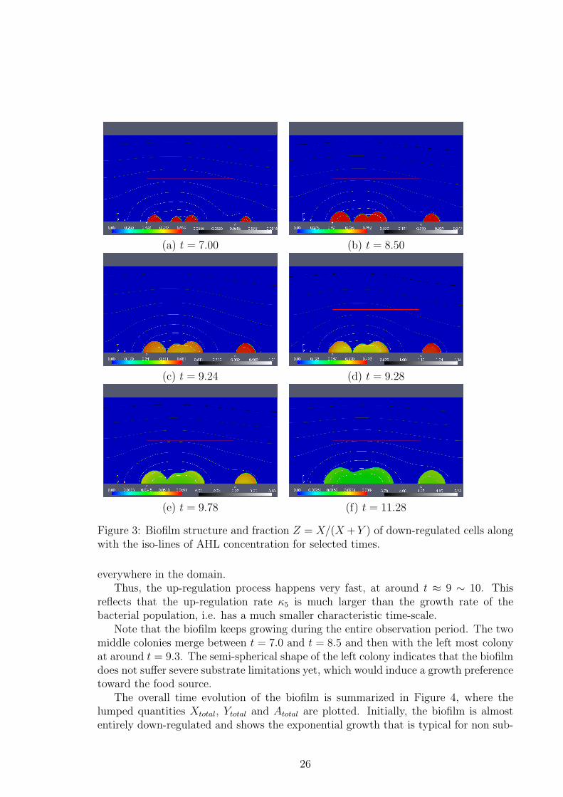
In Figure 3 we show for six time instances the biofilm structure, the AHL con-centration A, and the spatial composition of the biofilm from down- and up-regulatedbiomass X and Y . The latter is again represented in terms of the ratio of down-regulated biomass to total biomass, Z := X/(X + Y ) in Ω2(t) (while Z = 0 in Ω1(t)).In the first shown time step (a), at t = 7.00, all colonies are essentially down-regulated,due to the low AHL concentration A < 0.08. The AHL concentrations are largest in theinner layers of the biofilm colonies, close to the substratum. From the biofilm coloniesthe signaling molecules diffuse into to the aqueous phase. Similarly, at (b) t = 8.5with A < 0.247 the biofilm remains down-regulated. Note that between the first twoplotted time-steps all biofilm colonies continued growing and that the two colonies inthe middle of the substratum started merging. Induction starts at (c) t = 9.24, wherethe AHL concentration reaches A ≈ 1 in the clustered region where the colonies aredense, i.e. where more bacteria, and hence AHL producers, are concentrated. SomeAHL diffuses from the biofilm colonies into the aqueous phase. This diffusion loss ismore pronounced in the smaller isolated colony on the right than in the larger biofilmcluster region. In the clustered colonies, first the bacteria in the inner layers, close tothe substratum, upregulate and we observe a gradient of down-regulated cells from theinner layers to the biofilm/water interface in these colonies, i.e. a clearly heterogeneousdistribution of biomass within the biofilm. The fraction of down-regulated cells Z inthe clustered region of the biofilm is smaller than in the smaller isolated colony onthe right. Consequently, more AHL are produced there. This leads to a flux of AHLtoward the single colony, and thus contributes to an increase of up-regulation there.As a consequence, the up-regulation pattern in this nearly hemi-spherical colony is notsymmetric, but skewed toward the larger neighboring colony.
The next snapshot is taken shortly thereafter, at (d) t = 9.28, when the averageAHL concentration in the domain reaches the threshold value A ≈ 1. The pictureis qualitatively the same but more cells are now up-regulated in all colonies and theAHL concentration has risen to a maximum value of 1.36. The difference between thethree clustered colonies and the isolated colony is still clearly observable. Moreover,all colonies are still in a growing phase.
At (e) t = 9.78 AHL concentration A is everywhere in the domain clearly abovethe switching threshold 1. The colonies to the left merged. Only a small fraction ofcells in the biofilm colonies is still down-regulated, this fraction is slightly higher in theisolated colony to the right.
The fraction of down-regulated cells decreases even more until (f) t = 11.28, whereit only accounts locally for approximately 1% of the cells. The AHL concentration hasnow risen to a maximum value of 5.23 in the biofilm and a minimum value of 3.70
25
(a) t = 7.00 (b) t = 8.50
(c) t = 9.24 (d) t = 9.28
(e) t = 9.78 (f) t = 11.28
Figure 3: Biofilm structure and fraction Z = X/(X +Y ) of down-regulated cells alongwith the iso-lines of AHL concentration for selected times.
everywhere in the domain.Thus, the up-regulation process happens very fast, at around t ≈ 9 ∼ 10. This
reflects that the up-regulation rate κ5 is much larger than the growth rate of thebacterial population, i.e. has a much smaller characteristic time-scale.
Note that the biofilm keeps growing during the entire observation period. The twomiddle colonies merge between t = 7.0 and t = 8.5 and then with the left most colonyat around t = 9.3. The semi-spherical shape of the left colony indicates that the biofilmdoes not suffer severe substrate limitations yet, which would induce a growth preferencetoward the food source.
The overall time evolution of the biofilm is summarized in Figure 4, where thelumped quantities Xtotal, Ytotal and Atotal are plotted. Initially, the biofilm is almostentirely down-regulated and shows the exponential growth that is typical for non sub-
26

0
0.02
0.04
0.06
0.08
0.1
0.12
0 2 4 6 8 10 12 14 0
1
2
3
4
5
6
7
biom
ass
AH
L
t
XtotalYtotalAtotal
Figure 4: Evolution of the biofilm over time: shown is the amount of down- and up-regulated cells, as well as the amount of AHL in the system
strate limited systems. Autoinducers are produced at a low rate. Only at aroundt ≈ 9 enough AHL is accumulated to induce up-regulation. The switch from a mainlydown-regulated to a biofilm dominated by up-regulated cells is almost immediate. Thisswitch also induces a drastic jump in AHL accumulation due to the higher productionrate of up-regulated cells. After the switch has passed the population continues growingas an almost entirely up-regulated biofilm.
The simulations in Figure 3 show the effect of spatial arrangement of cell colonieson the biofilm. In other words, the switching behavior in one colony can be affectedby the size and location of other colonies. This supports the recent hypothesis ofefficiency sensing [12], which aims at combining quorum sensing in the strict sensewith the related concept of diffusion sensing. The former is commonly thought of asa mechanism to measure the size of the population, while the latter is thought of as amechanism to explore the spatial characteristics of the environment. Of course, botheffects are super-imposed, the AHL concentration measured by a cell depends on bothand both effects cannot be separated in this measurement. This together with thesimulations in the previous section shows the role that environmental conditions playfor quorum sensing, due to their effect on mass transfer.
In the previous study [10] the effect of convective transport of autoinducer moleculesin the bulk liquid on inter colony communication and up-regulation was studied. Oursimulations in the present article demonstrated that also the purely diffusive transportof autoinducers can affect the onset of switching greatly. In other words, spatial effectsare crucial in quorum sensing and can overwrite the meaning of quorum sensing in thestrict sense, namely the notion of quorum sensing as a mechanism by which bacteriasense the size of their population. In fact, under the influence of mass transport, AHLconcentrations are not a good indicator for population density, as they are alternatedby effects such as the spatial distribution of cells and the size and shape of the domainin which they live.
27
5 Conclusion
We studied a degenerate density-dependent diffusion-reaction system that models quo-rum sensing in bacterial biofilms. Our main analytical result is the well-posedness ofthe initial-boundary value problem. While similar existence proofs for models of thistype have been given previously, our work constitutes the first uniqueness result forsuch systems. This was possible because of a specific property of the quorum-sensingmodel, which previously studied models of other biofilm processes did not possess.More specifically, this property allowed us to make use of known uniqueness and reg-ularity results for the scalar case. Nevertheless, in forthcoming work we shall aim atextending the ideas underlying our uniqueness proof so that it becomes applicable toother systems as well.
In addition to the well-posedness proof, we showed computer simulations of thenumerical model, which indicated that quorum sensing in spatially structured biofilmscan be dominated by mass transfer effects. In other words, quorum sensing is not onlybased on cell numbers but also on their locations relative to each other, and on theboundary conditions. This ties in with the recently suggested concept of efficiencysensing, which combines quorum sensing in the strict sense with diffusion sensing as amechanism by which bacteria explore their spatial environment.
References
[1] V.V. Chepyzhov, M.I. Vishik, Attractors of Equations of Mathematical Physics,American Mathematical Society, Providence, Rhode Island, 2002.
[2] L. Demaret, H.J. Eberl, M.A. Efendiev, R. Lasser, Analysis and Simulation of aMeso-scale Model of Diffusive Resistance of Bacterial Biofilms to Penetration ofAntibiotics, Adv. Math. Sci. Appl. 18(1):269–304, 2008.
[3] M.A. Efendiev, L. Demaret, On the Structure of Attractors for a Class of Degen-erate Reaction-Diffusion Systems, Adv. Math. Sci. Appl. 18(1):105–118, 2008.
[4] H.J Eberl, S. Collinson, A modeling and simulation study of siderophore mediatedantagonism in dual-species biofilms, Theoretical Biology and Medical Modelling,6:30, 2009.
[5] H.J. Eberl, L. Demaret, A finite difference scheme for a degenerated diffusionequation arising in microbial ecology, Electronic Journal of Differential Equations,CS15:77–95, 2007.
[6] H.J. Eberl, D.F. Parker, M. van Loosdrecht, A new Deterministic Spatio-TemporalContinuum Model For Biofilm Development, J. of Theor. Medicine, 3(3)161–175,2001.
[7] H.J. Eberl, R. Sudarsan, Exposure of biofilms to slow flow fields: the con-vective contribution to growth and disinfection, Journal of Theoretical Biology,253(4):788-807, 2008.
28
[8] M.A. Efendiev, S. Sonner, Verifying Mathematical Models with Diffusion, Trans-port and Interaction, GAKUTO Internat. Series Math. Sciences and Appl., 3241–67, 2010.
[9] M.A. Efendiev, S. Zelik, H.J. Eberl, Existence and longtime behavior of a biofilmmodel, Communications on Pure and Applied Analysis, 8(2):509–531, 2009.
[10] M.R. Frederick, C. Kuttler, B.A. Hense, J. Muller, H.J. Eberl, A MathematicalModel of Quorum Sensing in Patchy Biofilm Communities with Slow BackgroundFlow, Can. Appl. Math. Quart., 18(3):267-298, 2010.
[11] M.R. Frederick, C. Kuttler, B.A. Hense, H.J. Eberl, A mathematical model ofquorum sensing regulated EPS production in biofilm communities, TheoreticalBiology and Medical Modelling, 8:8, 2011.
[12] B.A. Hense, C. Kuttler, J. Muller, M. Rothballer, A. Hartmann, Does efficiencysensing unify diffusion and quorum sensing?, Nature Reviews Microbiology, 5:230-239, 2007.
[13] Z. Lewandowski, H. Beyenal, Fundamentals of Biofilm research, CRC Press, BocaRaton, 2007.
[14] N. Muhammad, H.J. Eberl, OpenMP parallelization of a Mickens time-integrationscheme for a mixed-culture biofilm model and its performance on multi-core andmulti-processor computers, LNCS, 5976:180-195, 2010.
[15] N. Muhammad, H.J. Eberl, Model parameter uncertainties in a dual-speciesbiofilm competition model affect ecological ouptut parameters much stronger thanmorphological ones, submitted.
[16] J. Muller, C. Kuttler, B.A. Hense, M. Rothballer, A. Hartmann, Cell-cell com-munication by quorum sensing and dimension-reduction, Journal of MathematicalBiology, 53:672-702, 2006.
[17] A. Masic, J. Bengtsson, M. Christensson, Measuring and modeling the oxygenprofile in a nitrifying moving bed biofilm reactor, Math. Biosc. 227(1):1-11, 2010.
[18] J. Muller, C. Kuttler, B.A. Hense, M. Rothballer, A. Hartmann, Cell-cell Commu-nication by Quorum-Sensing and Dimension Reduction, J. Math. Biol., 53:672-702,2006.
[19] H. Khassehkhan, M.A. Efendiev, H.J. Eberl, A Degenerate Diffusion-ReactionModel of an Amensalistic Biofilm Control System: Existence and Simulation ofSolutions, Discrete Contin. Dyn. Syst. Ser. B 12(2):371–388, 2009.
[20] O.A. Ladyzhenskaya, V.A. Solonnikov, N.N. Uraltseva, Linear and Quasi-linearEquations of Parabolic Type, Nauka, Moscow, 1967; English transl., Amer. Math.Soc., Providence, RI, 1968.
29
[21] M. Renardy, R.C. Rogers, An Introduction to Partial Differential Equations,Springer-Verlag, New York, 1993.
[22] J. Smoller, Shock Waves and Reaction-Diffusion-Equations, Springer-Verlag, NewYork, 1983.
[23] O. Wanner, H. Eberl, O. Morgenorth, D. Noguera, D. Picioreanu, B. Rittmann,M. van Loosdrecht, Mathematical Modelling of Biofilms, IWAPublishing, London,2006.
30