one-dimensional flamestom/classes/641/cantera/workshop/flames.pdf · 7/25/04 cantera workshop ......

One-Dimensional Flames

David G. Goodwin

Division of Engineering andApplied Science

California Institute of Technology

7/25/04 Cantera Workshop

Several types of flames can be modeled as"one-dimensional"

A burner-stabilized flatflame

A premixedstagnation-pointflame

A non-premixedcounterflow flame


One-Dimensionality

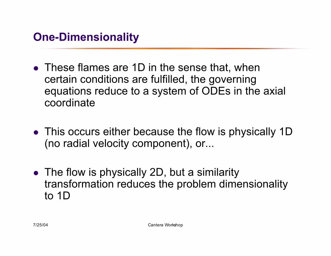
These flames are 1D in the sense that, whencertain conditions are fulfilled, the governingequations reduce to a system of ODEs in the axialcoordinate

This occurs either because the flow is physically 1D(no radial velocity component), or...

The flow is physically 2D, but a similaritytransformation reduces the problem dimensionalityto 1D


One-dimensional flames are only one typeof 1D reacting-flow problem

fuel inlet

gas flow

anode

electrolyte

cathode

gas flow

air inlet

Fuel cell test facility


Thin film deposition

showerhead

gas flow

film

Stagnation-flow chemicalvapor deposition reactor

surface

substrate


A "Stack" of domains

"Domains"

Cantera provides capabilities to solvegeneral axisymmetric 1D problems

Each domain represents a distinct phase, flowfield, or interface a gas flow an inlet or outlet a surface a solid ...


Multi-Physics Simulations

Physics may be different in each domain

Each domain has its own set of variables (components) andgoverning equations

Spatially-extended domains alternate with "connector" or"boundary" domains that provide the coupling

Solution determined for all domains simultaneously in fully-coupled, fully-implicit way


General Structure Applies for any 1D problem: flame, fuel cell stack, CVD

stagnation flow, ... A 1D problem is partitioned into domains

extended spatial domains define governing equations

gas 1 gas 2porousplug

boundary domains provide boundary / interfacial conditions

inlet fluxmatcher 1

fluxmatcher 2 surface

Example


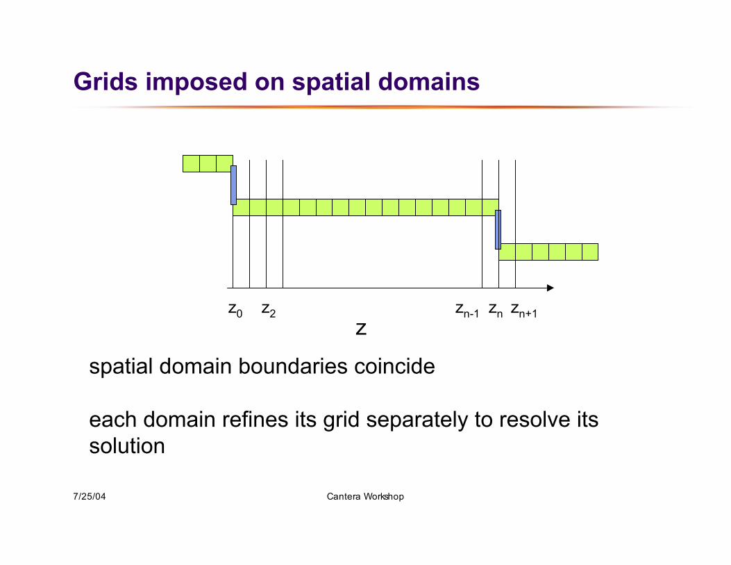
Grids imposed on spatial domains

zz0 z2 zn-1 zn zn+1

spatial domain boundaries coincide

each domain refines its grid separately to resolve itssolution


Domain Variables

Each type of domain has a specified set of variables at each gridpoint

Examples an axisymmetric flow domain -

K + 4 variables per point u, V, T, Λ, Y1, ..., YK

a surface domain K + 1 variables at one point only T, coverages of all surface species


Solution Vector

Domain 0 Domain m Domain M… …

Point 0 Point j Point Jm… …

φ = [ ]

Var 0 Var n Var Nm… …

Variables are ordered first by domain, then by point in the domain.Note that each domain m may have a different number of pointsJm, and a different number of variables per point Nm. All ordering isdone left-to-right.


Solution Method

Finite-difference flow equations to form a system ofnonlinear algebraic equations

Use a hybrid Newton / time-stepping algorithm tosolve the equations

Adaptively refine / coarsen grid to resolve theprofiles, or remove unnecessary points if over-resolved


Residual Function

In each domain, there is an equal number of equations andunknowns at each point

The nth equation at the jth point in the mth domain has theform

Fj,m,n(φ) = 0

where Fj,m,n depends only on solution variables at points j, j-1,and j+1

Therefore, the Jacobian of this system of equations isbanded.


The residual equations are solved using avariant of Newton’s Method

linearize about solution estimate ! (0) :

Flin,i

(0)= Fi (!

(0) ) +"Fi"! j !=!(0 )j

# (! j $! j

(0) )

solve linear problem to generate new estimate of !:

Flin (!(1) ) = 0,

! (1)= ! (0) $ J

(0)%& '($1

F(0)

where Ji, j = "Fi / "! j

Classical Newton's method:


Quadratic convergence

If F is linear, this leads to the exact solution φ∗ in 1step

If F is quadratic, then repeating this processproduces a convergent sequence of solutionestimates

with the error decreasing quadratically:

limn!"

# (n+1) $#* = A # (n) $#*2

! (0),! (1),! (2),! (3),...


Transient Problem

If Newton iteration fails to find thesteady-state solution, we attemptto solve a psuedo-transientproblem with a larger (perhapsmuch large) domain ofconvergence

This problem is constructed byadding transient terms in eachconservation equation where thisis physically reasonable

This may not be possible foralgebraic constraint equations;these are left unmodified

Ad

!

!

dt= F(!

!)

F(! (n+1) ) " A! (n+1) "! (n)

#t= 0

Let A be a diagonal matrixwith 1 on the diagonal forthose equations with atransient term, and 0 on thediagonal for constraintequations.

Then the modified problem isas shown above.


Transient Problem (cont'd)

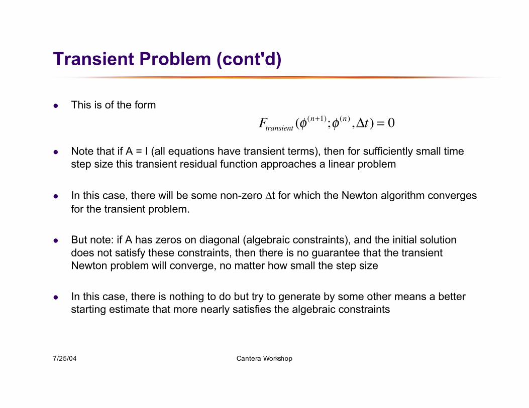
This is of the form

Note that if A = I (all equations have transient terms), then for sufficiently small timestep size this transient residual function approaches a linear problem

In this case, there will be some non-zero Δt for which the Newton algorithm convergesfor the transient problem.

But note: if A has zeros on diagonal (algebraic constraints), and the initial solutiondoes not satisfy these constraints, then there is no guarantee that the transientNewton problem will converge, no matter how small the step size

In this case, there is nothing to do but try to generate by some other means a betterstarting estimate that more nearly satisfies the algebraic constraints

Ftransient

(! (n+1);! (n),"t) = 0


Time step until solution enters s.s. domain ofconvergence, then proceed to solution using s.s. Newton

Take a few time steps

Try to solve steady-state problem

If not yet in steady-state domain ofconvergence, take afew more time steps

Repeat until steady-state Newton succeeds


A larger domain of convergence is achieved byusing a damped Newton method

Compute a Newton step

If the step carries the solution outside prescribed limits, determine thescalar multiplier required to bring it back in

Starting with this (possibly scaled) new solution vector,backtrack along the Newton direction until a point is found where thenext Newton step would have a smaller norm than the originalundamped, unscaled Newton step

If such a point can be found, accept the damped Newton step

Otherwise abort and try time-stepping for a while

Repeat until the solution converges, or a damped Newton step fails.


The Jacobian

By far the most CPU-intensive operation in this algorithm isevaluating the Jacobian matrix

Exact Jacobians are not required, so try to re-use previously-computed Jacobians

Only recompute J if: The damped Newton algorithm failed, and the Jacobian is out-of-date, or a specified maximum number of times it may be used has been reached

Note that switching between transient and steady-state modes onlyadds/subtracts a constant from the diagonal; no need to recomputeJacobian just to go from steady to transient or vise versa.


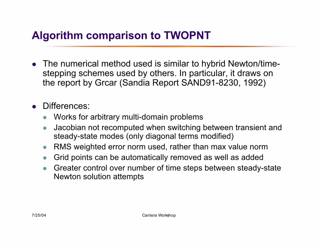
Algorithm comparison to TWOPNT

The numerical method used is similar to hybrid Newton/time-stepping schemes used by others. In particular, it draws onthe report by Grcar (Sandia Report SAND91-8230, 1992)

Differences: Works for arbitrary multi-domain problems Jacobian not recomputed when switching between transient and

steady-state modes (only diagonal terms modified) RMS weighted error norm used, rather than max value norm Grid points can be automatically removed as well as added Greater control over number of time steps between steady-state

Newton solution attempts

The AxisymmetricFlow DomainType

Python / MATLAB: classAxisymmetricFlow

C++: class AxiStagnFlow


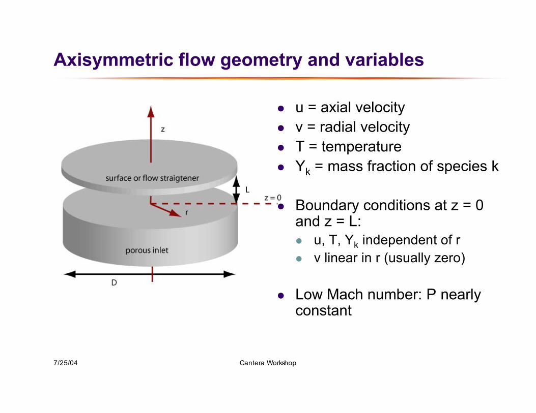
Axisymmetric flow geometry and variables

u = axial velocity v = radial velocity T = temperature Yk = mass fraction of species k

Boundary conditions at z = 0and z = L: u, T, Yk independent of r v linear in r (usually zero)

Low Mach number: P nearlyconstant


Similarity Solution

Consider the limits L/D << 1 Ma << 1

If these limits are satisfied, and if the boundary conditionsare satisfied, then the exact flow equations admit a solutionwith the properties: u = u(z) v = rV(z) T = T(z) Yk = Yk(z) P = P0 + Λr2/2.

Here Λ is a constant that must be determined as part of thesolution.


For conditions where similarity solution holds, flowequations reduce to ODEs in axial coordinate z


Upwind differencing for convective terms

if u j > 0 :

df

dz

!"#

$%&j

=f j ' f j'1

z j ' z j'1

otherwise:

df

dz

!"#

$%&j

=f j+1

' f j

z j+1' z j


Central differencing for diffusive terms


Axial velocity information flow

(!u)j+1

" (!u)j

#zj+1/2

+ (!V )j+ (!V )

j+1= 0

j j+1j-1

Continuity eq. propagatesinformation right-to-left

ρu specified on rightby right boundary object

burner-stabilized flame: zero gradientcounterflow flame: specified valuestagnation-point flame: zero


Lambda Equation

!j= !

j"1

j j+1j-1

Lambda eq. propagatesinformation left-to-right

Λ specified on leftby left boundary object

(!u)

0= !mleft

If mass flow rate from left is specified, then residualequation for Λ at left is

Flame Simulations in Python


Domain Class Hierarchy

Domain classes

Inlet Outlet Surface SymmPlane

Bdry1D

base class for boundary domains

AxisymmetricFlow

axisymmetric flow domains

Domain1D

base class for domains


Stack Class Hierarchy

BurnerFlame

burner-stabilized flames

CounterFlame

non-premixed counterflow flames

StagnationFlow

Stagnation flows with surface chemistry

Stack

base class for Stacks


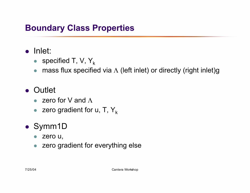
Boundary Class Properties

Inlet: specified T, V, Yk mass flux specified via Λ (left inlet) or directly (right inlet)g

Outlet zero for V and Λ zero gradient for u, T, Yk

Symm1D zero u, zero gradient for everything else


Surface Boundary Class

Surface species coverages

Coupling to gas Specified T, u = 0*, V = 0 Species:

*to be modified to handle the case of net mass deposition oretching

jk + !skWk = 0

!sj= 0


Flame Simulations in Python: a Burner-Stabilized Flame## FLAME1 - A burner-stabilized flat flame## This script simulates a burner-stablized lean# hydrogen-oxygen flame at low pressure.#from Cantera import *from Cantera.OneD import *

################################################################## parameter values#p = 0.05*OneAtm # pressuretburner = 373.0 # burner temperaturemdot = 0.06 # kg/m^2/s

rxnmech = 'h2o2.cti' # reaction mechanism filemix = 'ohmech' # gas mixture modelcomp = 'H2:1.8, O2:1, AR:7' # premixed gas composition

flame1.py


flame1.py

# The solution domain is chosen to be 50 cm, and a point very near the# downstream boundary is added to help with the zero-gradient boundary# condition at this boundary.initial_grid = [0.0, 0.02, 0.04, 0.06, 0.08, 0.1, 0.15, 0.2, 0.4, 0.49, 0.5] # m

tol_ss = [1.0e-5, 1.0e-13] # [rtol atol] for steady-state # problemtol_ts = [1.0e-4, 1.0e-9] # [rtol atol] for time stepping

loglevel = 1 # amount of diagnostic output (0 # to 5)

refine_grid = 1 # 1 to enable refinement, 0 to # disable


flame1.py

################ create the gas object ########################## This object will be used to evaluate all thermodynamic, kinetic,# and transport properties#gas = IdealGasMix(rxnmech, mix)

# set its state to that of the unburned gas at the burnergas.set(T = tburner, P = p, X = comp)

f = BurnerFlame(gas = gas, grid = initial_grid)

# set the properties at the burnerf.burner.set(massflux = mdot, mole_fractions = comp, temperature = tburner)


flame1.py

f.set(tol = tol_ss, tol_time = tol_ts)f.setMaxJacAge(5, 10)f.set(energy = 'off')f.init()f.showSolution()

f.solve(loglevel, refine_grid)

f.setRefineCriteria(ratio = 200.0, slope = 0.05, curve = 0.1)f.set(energy = 'on')f.solve(loglevel,refine_grid)

f.save('flame1.xml')f.showSolution()


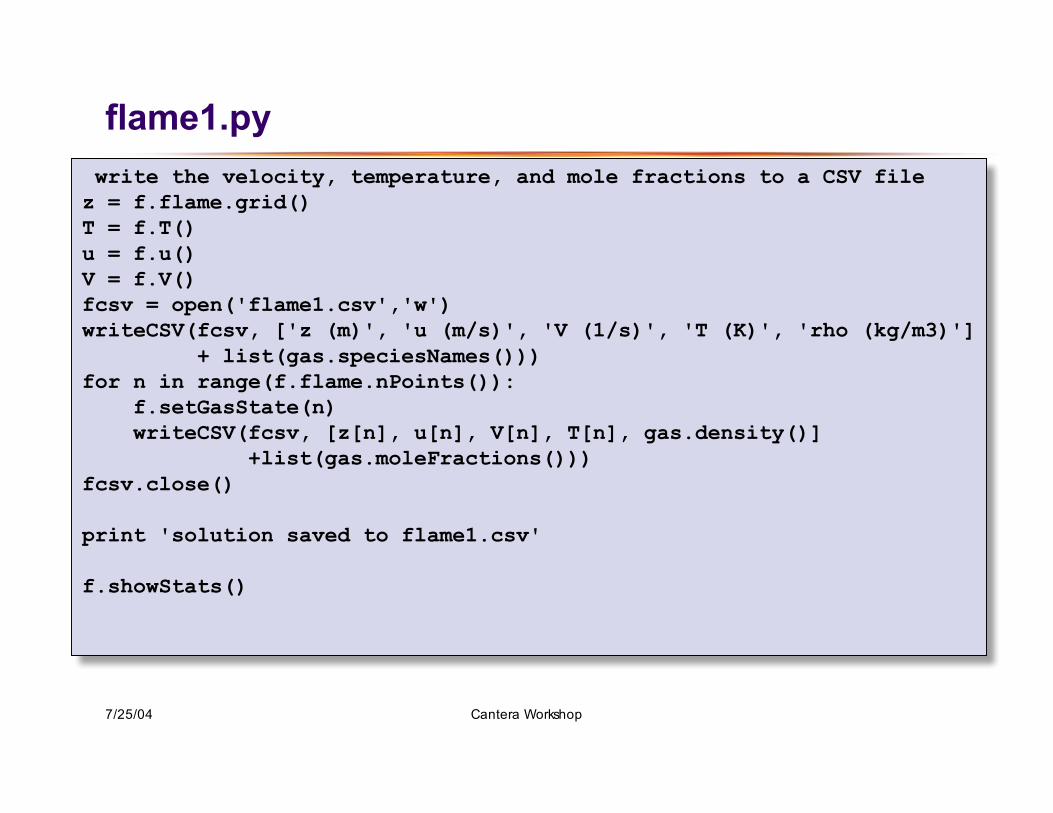
flame1.py write the velocity, temperature, and mole fractions to a CSV filez = f.flame.grid()T = f.T()u = f.u()V = f.V()fcsv = open('flame1.csv','w')writeCSV(fcsv, ['z (m)', 'u (m/s)', 'V (1/s)', 'T (K)', 'rho (kg/m3)'] + list(gas.speciesNames()))for n in range(f.flame.nPoints()): f.setGasState(n) writeCSV(fcsv, [z[n], u[n], V[n], T[n], gas.density()] +list(gas.moleFractions()))fcsv.close()

print 'solution saved to flame1.csv'

f.showStats()


Where to find files in the source distribution

C++ Directory Cantera/src/oneD

Python Modules in directory Cantera/python/Cantera/OneD Module onedim.py in this directory contains domain and stack classes Extension module source file ctonedim_methods.cpp in directory Cantera/python/src

MATLAB m-files in in directory Cantera/matlab/cantera/1D class Domain1D in Cantera/matlab/cantera/1D/@Domain1D class Stack in Cantera/matlab/cantera/1D/@Stack MEX source file Cantera/matlab/cantera/private/onedimmethods.cpp

clib File Cantera/clib/src/ctonedim.cpp

one-dimensional flamestom/classes/641/cantera/workshop/flames.pdf · 7/25/04 cantera workshop ......

Documents