Wright State University Wright State University

CORE Scholar CORE Scholar

Browse all Theses and Dissertations Theses and Dissertations

2020

One-Dimensional Kinetic Particle-In-Cell Simulations of Various One-Dimensional Kinetic Particle-In-Cell Simulations of Various

Plasma Distributions Plasma Distributions

Richard N. Vanderburgh Wright State University

Follow this and additional works at: https://corescholar.libraries.wright.edu/etd_all

Part of the Physics Commons

Repository Citation Repository Citation Vanderburgh, Richard N., "One-Dimensional Kinetic Particle-In-Cell Simulations of Various Plasma Distributions" (2020). Browse all Theses and Dissertations. 2395. https://corescholar.libraries.wright.edu/etd_all/2395

This Thesis is brought to you for free and open access by the Theses and Dissertations at CORE Scholar. It has been accepted for inclusion in Browse all Theses and Dissertations by an authorized administrator of CORE Scholar. For more information, please contact library-corescholar@wright.edu.

ONE-DIMENSIONAL KINETIC PARTICLE-IN-CELL

SIMULATIONS OF VARIOUS PLASMA

DISTRIBUTIONS

A thesis submitted in partial fulfillment of the

requirements for the degree of

Master of Science

By

RICHARD N. VANDERBURGH

B.S., Wright State University, 2019

2020

Wright State University

Wright State University

GRADUATE SCHOOL

December 2nd, 2020

I HEREBY RECOMMEND THAT THE THESIS PREPARED UNDER MY

SUPERVISION BY Richard N. Vanderburgh ENTITLED One-Dimensional

Kinetic Particle-In-Cell Simulations of Various Plasma Distributions BE

ACCEPTED IN PARTIAL FULFILLMENT OF THE REQUIREMENTS FOR

THE DEGREE OF Master of Science.

_________________________________

Amit Sharma, Ph. D.

Thesis Advisor

_________________________________

Jason Deibel, Ph. D.

Chair, Department of Physics

Committee on Final Examination

_________________________________

Amit Sharma, Ph. D.

_________________________________

Ivan Medvedev, Ph. D.

_________________________________

Sarah Tebbens, Ph. D.

_________________________________

Barry Milligan, Ph.D.

Interim Dean of the Graduate School

iii

ABSTRACT

Vanderburgh, Richard N. M.S. Department of Physics, Wright State University,

2020. One-Dimensional Kinetic Particle-In-Cell Simulations of Various Plasma

Distributions.

A one-dimensional kinetic particle-in-cell (PIC) MATLAB simulation was created

to demonstrate the time-evolution of various plasma distributions. Building on

previous plasma PIC programs written in FORTRAN and Python, this work

recreates the computational and diagnostic tools of these packages in a more user-

and educational-friendly development environment.

Plasma quantities such as plasma frequency and species charge-mass ratios are

arbitrarily defined. A one-dimensional spatial environment is defined by total

length and number and size of spatial grid points. In the first time-step, charged

particles are given initial positions and velocities on a spatial grid. After

initialization, the program solves for the electrostatic Poisson equation at each time

step to compute the force acting on each particle. Using the calculated force on

each particle and the “leap-frog” method, the particle positions and velocities are

updated and the motion is tracked in phase-space. Modifying parameters such as

spatial perturbation, number of particles, and charge-mass ratio of each species, the

time-evolution for various distributions are examined.

iv

The simulated distributions examined are categorized as the following: Cold

Electron Stream, Electron Plasma Waves, Two-Stream Electron Instability, Landau

Damping, and Beam-Plasma. The time evolution of the plasma distributions was

studied by several methods. Tracking the electric field, charge density and particle

velocities through each time step yields insight into the oscillations and wave

propagation associated with each distribution. One key diagnostic missing from the

original FORTRAN code was the electric field dispersion relation. The numerical

dispersion relation allows for further insight into modelling plasma

oscillations/waves in addition to the kinetic/field energies and electric field

tracking present in the original code. Simulated results show agreement with other

kinetic simulations as well as plasma theory.

v

TABLE OF CONTENTS

LIST OF FIGURES ............................................................................................................. vi

ACKNOWLEDGMENT ..................................................................................................... ix

Chapter1: Introduction .......................................................................................................... 1

Chapter 2: Particle-in-Cell (PIC) .............................................................................................. 5

2.1: Computational Cycle ....................................................................................................... 6

2.2: Integration of Equations of Motion ................................................................................. 6

2.3: Integration of the Field Equations ................................................................................... 9

2.4: Charge Density and Electric Field Weighting .................................................................. 11

Chapter 3: PIC Simulation Choice of Parameters and Diagnostics .......................................... 13

3.1: Plasma Parameters ....................................................................................................... 13

3.2: Waves in Plasma ........................................................................................................... 15

3.3 Plasma Energies ............................................................................................................. 18

Chapter 4: Plasma PIC Simulation Examples ......................................................................... 19

4.1 Cold Plasma Oscillations ................................................................................................. 19

4.2 Electron Plasma Waves .................................................................................................. 33

4.3 Two-Stream Instability ................................................................................................... 37

4.4 Landau Damping ............................................................................................................ 45

4.5 Beam-Plasma ................................................................................................................. 53

Chapter 5: Summary ............................................................................................................ 61

Bibliography ........................................................................................................................ 63

Appendix ............................................................................................................................. 65

vi

LIST OF FIGURES

Figure 1.1: Layers of the ionosphere differ by the altitude above the Earth. Depending on factors

like the altitude and time of day, the various layers will contain different temperatures and

densities of electrons and ionic species. The sun’s rays can excite ionic species which then

radiate, creating complicated behavior for computational modeling. [14] ............................. 2

Figure 1.2: Representation of a 1D electrostatic plasma model. Self and applied fields are along

the x-axis with no variation in either y or z. [1] ...................................................................... 3

Figure 2.1: PIC Mathematical spatial grid. Particles reside between gridpoints, but fields and

densities are calculated exclusively at the gridpoints. [2]....................................................... 5

Figure 2.1.1: Computational cycle for the PIC simulation. The particles are numbered i = 1, 2, …

NP; with grid indices j , which are scalers in 1D [2] ............................................................. 6

Figure 2.2.1: Leap-Frog Integration Scheme There are more accurate force integration

algorithms (the Runge-Kutta algorithm, for example) which can be implemented, at the cost

of higher computation demands, however. [2] ....................................................................... 8

Figure 2.3.1: Progression of charge density ρ(x) to ρ(k) to ϕ(k) finally to electrical potential

ϕ(x) [2] ................................................................................................................................. 10

Figure 2.3.2: Example Plots taken from a Cold Plasma Using MATLAB. The plots show the

progression from charge density 𝜌(𝑥) to 𝜌(𝑘) to 𝜙(𝑘) finally to electrical potential in real

space, 𝜙(𝑥). ........................................................................................................................... 10

Figure 2.4.1: Effective particle shape as seen by the spatial grid [8] ........................................... 11

Figure 3.2.1: Example of a Theoretical Plasma Dispersion Relation ........................................... 17

Figure 4.1.1: The cold plasma phase space shows the initial uniformity of the distribution

function, which then oscillates with a sinusoidal standing wave. Each electron possesses

simple harmonic motion around its respective initial position ............................................. 20

Figure 4.1.2: The Cold Plasma initially possesses a sinusoidal charge density due to the spatial

perturbation, then oscillates harmonically for the duration of the simulation [4] ................ 21

Figure 4.1.3: The electric field oscillation behaves similar to the charge density oscillation, as the

electrostatic model means that the electric field is merely the negative of the charge

density’s derivative in space ................................................................................................. 22

Figure 4.1.4: Cold Plasma Energies show a periodic exchange between the kinetic and potential

energies, tracking the total energy demonstrates the non-conserving property of this

simulation .............................................................................................................................. 22

Figure 4.1.5: This plot shows the cold plasma energies of another simulation. [6] .................... 24

Figure 4.1.6: With an initial spatial perturbation mode set to 1, the modal electrostatic energies of

the cold oscillation are found using Equation 3.3.5 [2] ........................................................ 25

Figure 4.1.7: Cold plasma electrostatic modal energies with a spatial perturbation mode set to 2.

The electrostatic mode with the highest energy corresponds to the spatial perturbation mode

in this example ...................................................................................................................... 26

Figure 4.1.8: Electrostatic modal energies with excitation of mode 3.......................................... 27

Figure 4.1.9: Theoretical dispersion relation for a cold plasma, found analytically using the fluid

continuity and momentum conservation equations combined with the conditions of a cold

plasma. [2] ............................................................................................................................ 28

Figure 4.1.10: Cold plasma numerical dispersion relation with 𝜔𝑝=1 and spatial perturbation

mode=1 ................................................................................................................................. 29

vii

Figure 4.1.11: This numerical dispersion plot is taken from another PIC simulation. The

disagreement between the theoretical black line and Fourier amplitudes may be be due to

the chosen parameters. [6] .................................................................................................... 30

Figure 4.1.12: Cold plasma numerical dispersion relation with 𝜔𝑝=2 and spatial perturbation

mode=1 ................................................................................................................................. 31

Figure 4.1.13: Cold plasma numerical dispersion relation with 𝜔𝑝=2 and spatial perturbation

mode=2 ................................................................................................................................ 31

Figure 4.1.14: Cold plasma numerical dispersion relation with 𝜔𝑝=3 and mode=2 ................... 32

Figure 4.2.1: Theoretical dispersion relation for Electron Plasma Waves [3] .............................. 33

Figures 4.2.2: Numerical Dispersion Relation of Electron Plasma Waves with theoretical curve

for comparison ..................................................................................................................... 35

Figures 4.2.3: Numerical dispersion relation of electron plasma waves. [5] ............................... 35

Figures 4.2.4: Dispersion relation of electron plasma waves of 𝜔𝑝 =2 ....................................... 36

Figures 4.2.5: Dispersion relation of electron plasma waves of 𝜔𝑝 =2 ........................................ 36

Figure 4.3.1 Phase-space time evolution of two-stream instability ............................................. 39

Figure 4.3.2 Two-stream time evolution of charge density ......................................................... 39

Figure 4.3.3: Two-stream electric field time evolution ................................................................ 40

Figure 4.3.4: Two-stream kinetic, electric potential, and total energies ....................................... 41

Figure 4.3.5: Time evolution of the electrostatic modal energies, with most of the energy in the

excited mode 1 until the instability reaches maximum electric field. After this point in time

the streams become thermalized and the other modes developed comparable energies ..... 42

Figure 4.3.6: The two-stream velocity distribution time evolution shows divergence in the

velocities after approximately time=10 (arbitrary units). Thermalization is reached at about

time=30, as the velocity distribution starts to possess a Maxwellian shape ......................... 43

Figure 4.3.7: Drift energies for each electron stream. Both streams possess identical energies for

each case. The drift energies initially hold at a steady value, until maximum instability,

when the thermal energy takes over...................................................................................... 44

Figure 4.3.8: Time evolution of the thermal energies of each steam show identical behavior

between the two streams. During the exponential increase in electric field, the velocities

start to become thermalized simultaneously ......................................................................... 45

Figure 4.4.1: Initial distribution function represented in phase space. As opposed to the cold

plasma and two-stream examples, and similar to the electron plasma waves, the electrons

are given an initial Maxwellian velocity distribution ........................................................... 47

Figure 4.4.2: Looking at the charge density evolution, the initially rough sinusoidal shape

quickly decays and loses coherence due to Landau damping ............................................... 48

Figure 4.4.2: Looking at the charge density evolution, the initially rough sinusoidal shape

quickly decays and loses coherence due to Landau damping ............................................... 49

Figure 4.4.4: The time evolution of the velocity distribution shows how the Maxwellian shape is

virtually unchanged while the electric field decays .............................................................. 50

Figure 4.4.5: The thermal energy of the Landau damping example shows an initial increase in

thermal energy, coinciding with the loss of electrostatic field energy in Figure 4.4.6 ......... 51

Figure 4.4.6: The electrostatic field energy shows an exponentially decaying oscillation,

characteristic of Landau Damping of the electric field ......................................................... 52

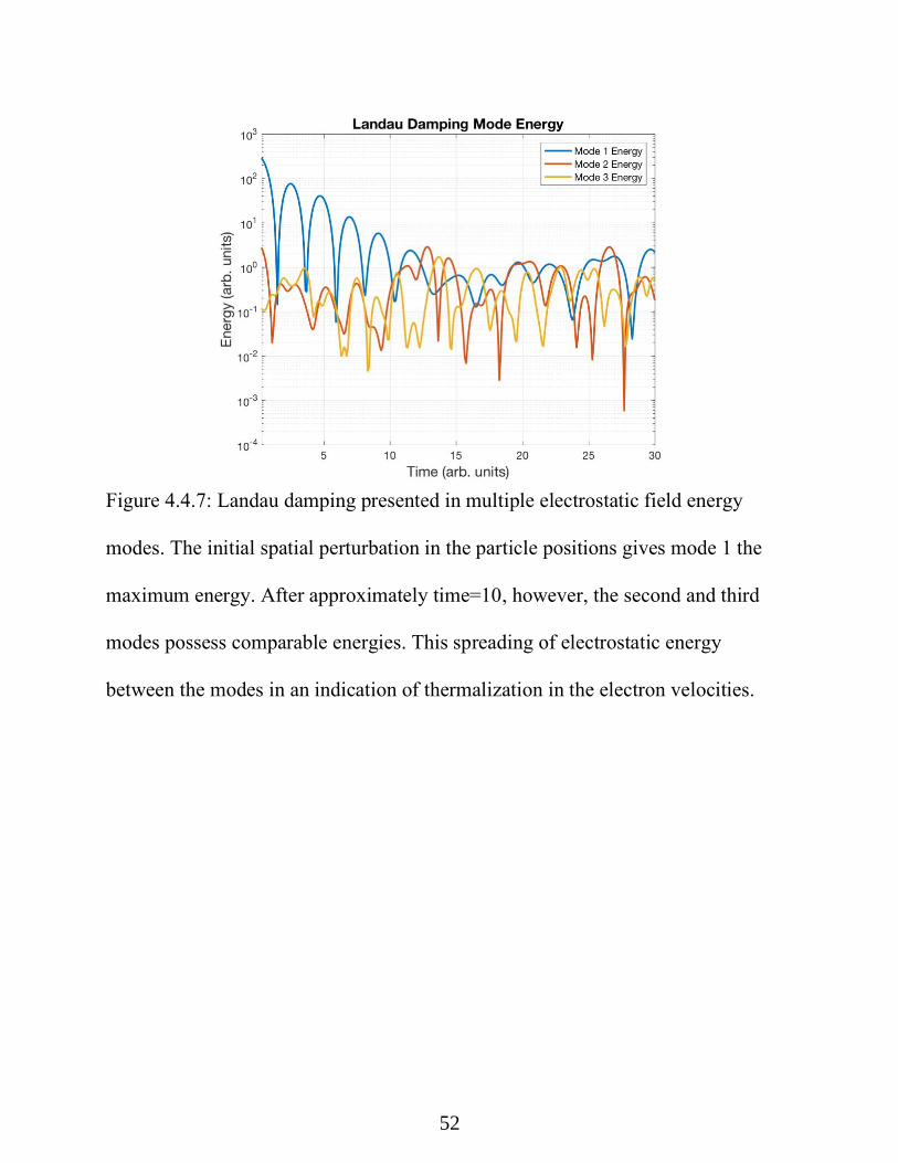
Figure 4.4.7: Landau damping presented in multiple electrostatic field energy modes. The initial

spatial perturbation in the particle positions gives mode 1 the maximum energy. After

approximately time=10, however, the second and third modes possess comparable energies.

viii

This spreading of electrostatic energy between the modes in an indication of thermalization

in the electron velocities ....................................................................................................... 53

Figure 4.5.1: The beam-plasma phase space shows a similar behavior as the two- stream

example. The blue dots represent mobile electrons with an initial drift velocity of 1. The red

dots represent ions with a much lower charge-mass ratio .................................................... 55

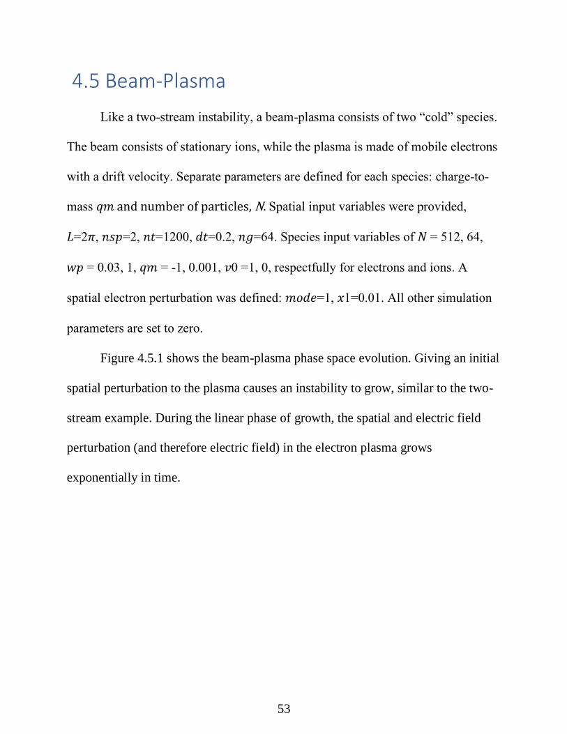
Figure 4.5.2: The beam-plasma electric field time evolution shows a mostly sinusoidal shape, as

the electrons are the primary factor in electric field. Electrons are much higher in number

and have a much higher plasma frequency, the computer parameter which determines

charge and mass when combined with the charge-mass ratio .............................................. 56

Figure 4.5.3: Similar to the two-stream, the electrostatic field energy increases exponentially

until about time=110. After this time, the field energy starts to oscillate, exchanging

primarily with the electrons’ kinetic energy ........................................................................ 57

Figure 4.5.4: The modal electrostatic field energies show that the first mode is dominant, as the

electrons are spatially perturbed to excite that wavelength .................................................. 58

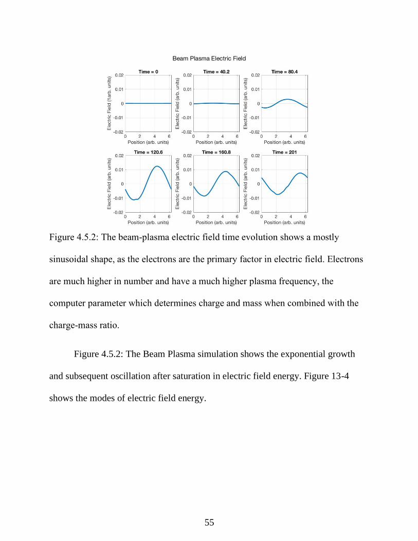
Figure 4.5.5: The time evolution of the beam-plasma velocity distribution shows that the he

heavy ions maintain their velocities much more than the electron plasma, which starts to

develop a Maxwellian distribution near the end of the run .................................................. 59

Figure 4.5.6: The thermal energies of both the electrons and ions increase exponentially,

coinciding with the increase in electric field ........................................................................ 60

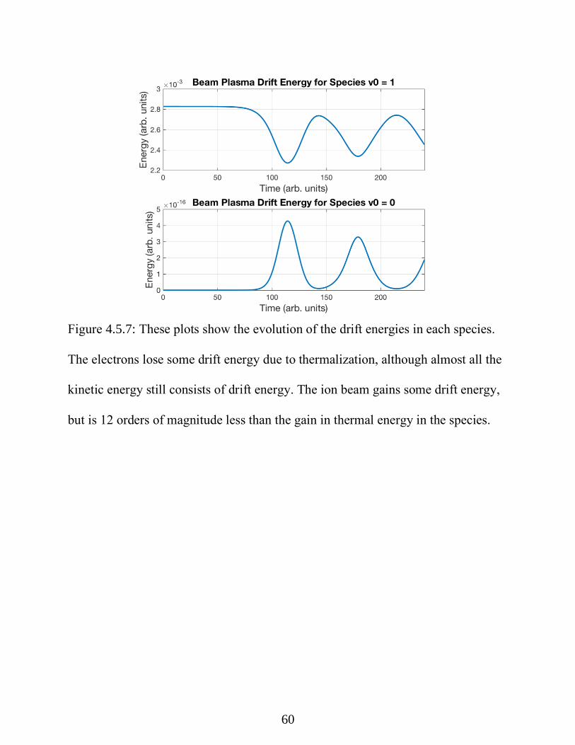
Figure 4.5.7: These plots show the evolution of the drift energies in each species. The electrons

lose some drift energy due to thermalization, although almost all the kinetic energy still

consists of drift energy. The ion beam gains some drift energy, but is 12 orders of

magnitude less than the gain in thermal energy in the species ............................................ 61

Figure 4.5.8: Most of the electrons’ kinetic energy consists of drift energy, as the species is given

an initial drift velocity. The rest of the electron kinetic energy is thermal velocity, which can

be seen in Figure 4.5.7. Most of the ions’ kinetic energy consists of thermal energy, which

can be seen in Figure 4.5.6 ................................................................................................... 62

ix

ACKNOWLEDGMENT

I would like to give a great thanks to my thesis advisor Dr. Amit Sharma.

His patience in assisting with this work, particularly with learning how to interpret

FORTRAN code, was invaluable. Thank you to Dr. Sarah Tebbens for additional

help with deciphering the FORTRAN code. Thank you to Dr. Thomas Skinner for

proofreading my document and providing critical feedback. Thank you to Dr.

Medvedev for participating in my thesis advising committee in addition to Dr.

Sharma and Dr. Tebbens. I also have a special thank you to all Wright State

Physics Professors and Faculty, for enriching my Physics Education and

inspiration for seeing this project to completion.

1

Chapter 1: Introduction

Plasma is often considered the fourth state of matter. As opposed to classical

electrically neutral gas, plasma is composed of ionized gas molecules and

electrons. Most of the observable universe consists of matter in the form of plasma:

stars, intergalactic dust, lightning, and even some parts of the Earth’s atmosphere.

In modern times, engineers and scientists have harnessed plasma for the

development of technologies such as neon signs, fluorescent lights, semiconductor

etching, and tokamaks (a device which uses magnetic confinement to produce

controlled thermonuclear fusion power).

The ionosphere is the ionized region of Earth’s atmosphere, consisting of

ions and other charged particles. Therefore, this region possesses plasma-like

characteristics. Between altitudes of 60-1,000 km, most of the ionization in this

layer is provided by the sun. When radio waves are sent through the atmosphere,

the ionosphere interacts with the signal due to the electromagnetic interaction. One

effect of this interaction is the absorption/reflection of radio signals due to ions. [1]

Figure 1.1 shows the various regions of the Earth’s ionosphere. Each region

is characterized by the temperature and density of electrons and ionic species

present. The interaction of space/terrestrial satellite communications (SATCOM)

with the ionosphere depends on the layer of propagation, as each layer possesses

unique electromagnetic properties.

2

Figure 1.1: Layers of the ionosphere differ by the altitude above the Earth.

Depending on factors like the altitude and time of day, the various layers will

contain different temperatures and densities of electrons and ionic species. During

the day, the sun’s rays excite gaseous molecules, which then radiate. The formation

of these ionic species produces complicated behavior for computational modeling.

[14]

In a plasma simulation, SATCOM signals may be represented by a

perturbation in a charge distribution. Through defining an initial setup of plasma

parameters and initial distribution, the time evolution is approximated through

computation of equations of motion and electromagnetic interaction.

3

For a fully physical representation of any arbitrary plasma distribution, any

number of particles must be tracked through time according to position, velocity,

and acceleration. Representing the plasma particles in phase space, particle

positions and velocities are tracked in space and time. A 1-dimensional

representation is often sufficient to demonstrate real physics. Figure 1.2 shows a

one-dimensional plasma consisting of sheet-charges, which are non-uniform

exclusively along the x-direction.

Figure 0.2: Representation of a 1D electrostatic plasma model. Self and applied

fields are along the x-axis with no variation in either y or z. [1]

Although this work does not model plasma phenomenon unique to the

ionosphere, the simple examples demonstrated are necessary steps to building a

fully physical code.

4

In addition to theoretical and experimental research, computational

simulations have yielded powerful results in understanding plasma physics. Within

the realm of plasma simulation, the methods used for various physical situations

can be broken into two groups—kinetic and fluid. Kinetic models are suitable for

calculating the motion of discrete particles interacting with electric and magnetic

fields. The drawback to kinetic models has historically been the heavy

computational requirements, as opposed to a fluid simulation. The benefit of a

kinetic simulation is the ability to resolve microscopic particle effects, which are

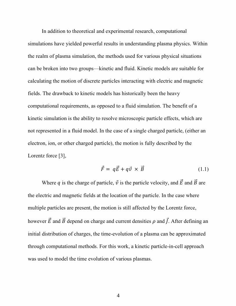
not represented in a fluid model. In the case of a single charged particle, (either an

electron, ion, or other charged particle), the motion is fully described by the

Lorentz force [3],

�⃗� = 𝑞�⃗⃗� + 𝑞𝑣 × �⃗⃗� (1.1)

Where 𝑞 is the charge of particle, 𝑣 is the particle velocity, and �⃗⃗� and �⃗⃗� are

the electric and magnetic fields at the location of the particle. In the case where

multiple particles are present, the motion is still affected by the Lorentz force,

however �⃗⃗� and �⃗⃗� depend on charge and current densities 𝜌 and 𝐽. After defining an

initial distribution of charges, the time-evolution of a plasma can be approximated

through computational methods. For this work, a kinetic particle-in-cell approach

was used to model the time evolution of various plasmas.

5

Chapter 2: Particle-in-Cell (PIC)

Calculation of the motions and fields of the plasma particles requires a

spatial grid to track the positions, as well as the charge and current densities of the

distribution. Figure 2.1 shows an arbitrary 2-dimensional plasma distribution with

a spatial grid defined by Cartesian x and y coordinates. [2]

Figure 2.1: PIC Mathematical spatial grid. Particles reside between grid points, but

fields and densities are calculated exclusively at the grid points. [2]

Particles with charge and mass can travel between the gridlines, however,

electric and magnetic fields are calculated along the gridlines exclusively.

6

2.1: Computational Cycle

The “leap-frog” method allows for a computationally efficient method of

integration. Figure 2.1.1 shows the sequence in the cycle of computation. First, the

simulation parameters (particle positions, velocities, etc.) are defined. Next, a

weighting method is used to calculate charge and current densities 𝜌 and J along

the gridlines. Integration of these densities yields the electric and magnetic fields E

and B. These fields are then weighted along the gridlines to find the force F for

each particle.

Figure: 2.1.1: Computational cycle for the PIC simulation. The particles are

numbered i = 1, 2, … NP; with grid indices j , which are scalers in 1D [2]

s

7

2.2: Integration of Equations of Motion

The first-order differential equations of motion for each particle are shown

in Equation’s 2.2.1 and 2.2.2. The force �⃗⃗⃗� becomes a scaler in 1-dimension and

only depends on the charge 𝑞 of each particle and electric field 𝑬. [2]

𝑚𝑑�⃗⃗⃗�

𝑑𝑡= �⃗⃗⃗� = 𝑞𝑬 (2.2.1)

𝑑�⃗⃗⃗�

𝑑𝑡= �⃗⃗⃗� (2.2.2)

These equations are replaced by the finite-difference equations,

𝑚�⃗⃗⃗�𝑛𝑒𝑤−�⃗⃗⃗�𝑜𝑙𝑑

∆𝑡= �⃗⃗⃗�𝑜𝑙𝑑 (2.2.3)

and

�⃗⃗⃗�𝑛𝑒𝑤−�⃗⃗⃗�𝑜𝑙𝑑

∆𝑡= �⃗⃗⃗�𝑛𝑒𝑤 (2.2.4)

Figure 2.2.1 shows the “leap-frog” integration method and time-centering.

The computer advances 𝒗𝒕⃗⃗ ⃗⃗ , and �⃗⃗⃗�𝒕 to �⃗⃗⃗�𝒕+∆𝒕 and �⃗⃗⃗�𝒕+∆𝒕 even though the initial

positions and velocities are not known at the same time. The initial conditions for

particle velocities and positions given at t = 0 must be changed to fit in the flow of

time. First, 𝒗𝟎⃗⃗ ⃗⃗⃗ is pushed back to �⃗⃗⃗�−∆𝒕/𝟐 using the force �⃗⃗⃗� calculated at t=0.

Second, the energies calculated from 𝒗𝒕⃗⃗ ⃗⃗ (kinetic) and �⃗⃗⃗�𝒕 (electric field potential)

must be adjusted to appear at the same time. The leap-frog method has error, with

the error vanishing as ∆𝑡 → 0. This work uses the “leap-frog” method in all the

8

examples, because it is both simple (easy to understand, and with minimum

storage) and surprisingly accurate [2].

Figure 2.2.1: Leap-Frog Integration Scheme. There are more accurate force

integration algorithms (higher-order Runge-Kutta methods, for example) which

can be implemented, at the cost of higher computation demands, however. [2]

9

2.3: Integration of the Field Equations

For the electrostatic case, the differential equations to solve are

�⃗⃗⃗� = −�⃗⃗⃗�𝝓 or 𝑬𝑥 = −𝜕𝜙

𝜕𝑥 and �⃗⃗⃗� ∙ �⃗⃗⃗� =

𝝆

𝝐𝟎 or

𝜕𝑬𝑥

𝜕𝑥=

𝝆(𝒙)

𝝐𝟎

This set of differential Maxwell’s equations are solved for the Electrostatic Case

[2]. When combined, these equations provide Poisson’s equation to provide the

formula for electrostatic potential. [2]

𝛁𝟐𝝓 = −𝝆(𝒙)

𝝐𝟎 or

𝜕2𝝓𝑥

𝜕𝑥2 = −𝝆(𝒙)

𝝐𝟎 (2.3.1)

There are numerous approaches to solving Poisson’s equation, one being a

solution using discrete Fourier transforms. For this approach to be feasible, we

enforce periodic boundary conditions. If a particle moves left of 0, then it is placed

on the opposite side of the numerical grid, at L. If the particle moves right of L, the

reverse happens, and is placed back at 0. The Fourier transform of charge density

provides the following identity between potential and charge density in k-space.

𝝓(𝑘) =𝝆(𝒌)

𝝐𝟎𝒌𝟐 (2.3.2)

The formula above is used to obtain potential from charge density using

Fourier Transform, where the 𝜕2

𝜕𝑥2 operator has been replaced by −𝑘2. Next, an

inverse Fourier transform is performed to solve for 𝝓(𝑥). The last step is to find

the grid’s electric field from the negative gradient of the electric potential. The

10

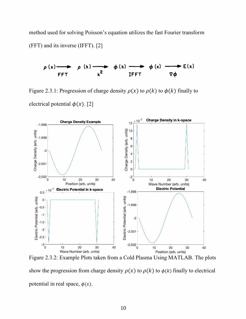
method used for solving Poisson’s equation utilizes the fast Fourier transform

(FFT) and its inverse (IFFT). [2]

Figure 2.3.1: Progression of charge density 𝜌(𝑥) to 𝜌(𝑘) to 𝜙(𝑘) finally to

electrical potential 𝜙(𝑥). [2]

Figure 2.3.2: Example Plots taken from a Cold Plasma Using MATLAB. The plots

show the progression from charge density 𝜌(𝑥) to 𝜌(𝑘) to 𝜙(𝑘) finally to electrical

potential in real space, 𝜙(𝑥).

11

2.4: Charge Density and Electric Field Weighting

Calculation of the force acting on each plasma particle requires defining the

charge density grid point. Depending on the desired level of accuracy, different

weighting schemes are used. The most simple weighting schemes are known as

nearest-grid-point (NGP) and cloud-in-cell (CIC). Figure 2.4.1 shows the particle

shape “as seen by the spatial grid”.

Figure 2.4.1: Effective particle shape as seen by the spatial grid [8]

Although the NGP scheme is computationally simple, the calculation yields

a square particle shape as “seen by the grid” as a square. This all-or-nothing

12

method deposits charge density in the cell closest to the particle. Using the first-

order CIC weighting yields a triangular particle shape as “seen by the grid”. This

method deposits charge density at not just a single cell, but the next closest cell as

well.

NGP: 𝜌𝑖 =𝑞

∆𝑥 (2.4.1)

CIC: {𝜌𝑖 =𝑞

∆𝑥 [

𝑋𝑖+1−𝑥

∆𝑥] =

𝑞

∆𝑥 [

𝑋𝑖+∆𝑥−𝑥

∆𝑥]} and {𝜌𝑖+1 =

𝑞

∆𝑥} (2.4.2)

Equations 2.4.1 and 2.4.2 show the Nearest-Grid-Point and Cloud-In-Cell

Weighting Schemes [2]

It should be noted that all plasma simulation examples in this work are

implemented using CIC. Similar to the charge density weighting, the electric field

acting on each particle is calculated using a linear weighting on the jth cell from

each for each ith particle.

𝐸𝑖 = [1 − (𝑥

∆𝑥− 𝑗)] 𝐸𝑗 + [

𝑥

∆𝑥− 𝑗]𝐸𝑗+1 (2.4.3)

Equation 2.4.3 shows the electric field weighting used for all examples shown [2]

13

Chapter 3: PIC Simulation Choice of Parameters and Diagnostics

3.1: Plasma Parameters

To guarantee the PIC simulation obeys real physics, fundamental plasma

parameters must be considered. One of the most fundamental plasma parameters is

known as the plasma frequency, 𝜔𝑝. [3]

𝜔𝑝 = √𝑛𝑞𝑚

2

𝜖0𝑚 (3.1.1)

Equation 3.1.1 shows the formula for a plasma frequency of electrons

against neutralizing background species. In all the examples in this work, the

plasma frequency is defined to calculate the mass m and charge q from the

arbitrarily defined charge-to-mass ratio q/m.

𝑞 = 𝐿 ∗ 𝜔𝑝

𝑒𝑝𝑠𝑖 ∗ 𝑁 ∗ 𝑞/𝑚

𝑚 = 𝑞

𝑞/𝑚

Another fundamental plasma parameter is known as the Debye Length, 𝜆𝐷.

This is defined as the distance traveled by a particle at the thermal velocity in 1/ 2𝜋

of a plasma cycle. It can be interpreted as the shielding distance around a test

charge and the scale length inside which particle-particle effects occur most

strongly and outside of which collective effects dominate. This constrains the

14

spatial grid size to be dependent on the arbitrary thermal velocity and plasma

frequency.

𝜆𝐷 =𝑣𝑡ℎ𝑒𝑟𝑚𝑎𝑙

𝜔𝑝→ ∆𝑥 ≈ 𝜆𝑑 (3.1.2)

Equation 3.1.2 shows the formal definition of the Debye Length, leading to a

constrained spatial grid size. This work focusses on the collective behavior of

collisionless plasmas at wavelengths longer than the Debye length, 𝜆 ≥ 𝜆𝐷. [2]

The useful information in a one-dimensional simulation is significantly less

computationally intensive than a three-dimensional case. Instead of modeling the

three-dimensional number of particles, 𝑁𝐷 ≈ 106, the one-dimensional 𝑁𝐷 ≈ 102

is used. A collisionless plasma is characterized by 𝑁𝐷 ≫ 1 and 𝐿 ≫ 𝜆𝐷. [2]

In order to obtain time-dependent oscillations in the plasma simulation, an

initial spatial perturbation is defined:

𝑥1cos(2𝜋 𝑥𝑖𝑚𝑜𝑑𝑒

𝐿+ 𝜃𝑥) (3.1.3)

Where 𝑥1is the amplitude and 𝑥𝑖 is the position of the ith particle. This

creates bunching in some areas of the plasma distribution, and greater separation

between charges in other areas. In areas where the bunching is tighter, the electric

field will push the particles away from each other.

15

3.2: Waves in Plasma

To demonstrate the wave phenomenon of a plasma, a fluid formulation is

used to derive the equations. Fluid models describe many of the fundamental

results of plasma physics, including the phenomena demonstrated by the examples

shown in this paper. In this work, a fluid approach is used to derive the dispersion

of two examples: cold plasma oscillations and electron plasma waves.

The first equations needed for the derivations are the continuity and

momentum equations. For every species s present in the plasma, there is a plasma

fluid continuity equation, [3]

𝜕𝑛𝑠

𝜕𝑡+ ∇ ∙ (𝑛𝑠𝒗𝑠) = 0 (3.2.1)

and the plasma fluid momentum equation,

𝑛𝑠 = (𝜕𝒗𝑠

𝜕𝑡+ (𝒗𝑠 ∙ ∇)𝒗𝑠) =

𝑞𝑠𝑛𝑠

𝑚𝑠(𝑬 + 𝒗𝑠 × 𝑩) −

𝛾𝑘𝐵𝑇𝑠

𝑚𝑠∇𝑛𝑠 (3.2.2)

Where 𝑛𝑠 and 𝒗𝑠 are the particles’ density and velocity of species s, q and m

are its individual particles’ charge and mass, and T is the temperature of the

particle species. Since this work is only looks at the electrostatic case, solving for

the wave phenomenon only requires Poisson’s equation combined with equations

3.2.1 and 3.2.2, whereas a fully electromagnetic model would incorporate

Faraday’s and Ampere’s Laws as well.

16

The periodic motion of the plasma examples discussed in this work is

expressed through Fourier analysis as a superposition of sinusoidal oscillations

with frequencies 𝜔 and wavelengths 𝜆. The simplest wave is a single component of

this decomposition. When the oscillation amplitude is small, a waveform is mostly

sinusoidal; and there is only one component.

A sinusoidal oscillation, for example, in the electric field—is represented by

Equation 3.2.3. [3]

𝐸(𝒓, 𝑡) = 𝐸0 𝑒𝑥𝑝[𝑖(𝒌 · 𝒓 − 𝜔𝑡)] (3.2.3)

Where

𝒌 · 𝒓 = 𝑘𝑥𝑥 + 𝑘𝑦𝑦 + 𝑘𝑧𝑧 (3.2.4)

Looking at only the x-component of the wave propagation, 𝐸(𝒙, 𝑡), a two-

dimensional FFT of the electric field data in space in time is used to obtain electric

field as a function of 𝑘 and 𝜔. The calculation of the 𝑘 and 𝜔 Fourier amplitudes is

then compared to the theoretical dispersion to assess the accuracy of the physics

shown by the PIC simulation.

Figure 3.2.1 shows an example of a plasma dispersion relation. The diagram

depicts the dependency of angular frequency 𝜔 with wave number k of an electron

plasma wave. This system will be discussed more thoroughly in Chapter 4.2.

Depending on the classification of wave, different mathematical dependencies are

derived for the dispersion relation. Equations 3.2.5 and 3.2.6 show the phase

17

velocity and group velocities 𝑣𝜙 and 𝑣𝑔 as functions of 𝜔 and k. If a wave

possesses a dispersion relation with 𝑣𝑔= 0, the curve will be characterized as

having a horizontal slope, as 𝑣𝑔 =𝑑𝜔

𝑑𝑘 = 0. In this case, there is no wave

propagation. If the dispersion relation has a non-zero slope, then the wave

propagates. As a check to make sure a wave follows real physics, 𝑣𝑔 must be less

than the speed of light, and therefore the largest allowed 𝜔 is ck.

𝑣𝜙 =𝜔

𝑘 (3.2.5)

𝑣𝑔 =𝑑𝜔

𝑑𝑘 (3.2.6)

Figure 3.2.1: Example of a Theoretical Plasma Dispersion Relation

18

3.3 Plasma Energies

Calculation of various kinetic and potential energies yield further insight

into the plasma characteristics. The total kinetic energy for each species is defined

by the following equation at each time step.

𝐾𝐸𝑠𝑝𝑒𝑐𝑖𝑒𝑠 =1

2∑ 𝑚𝑖𝑣𝑖

2𝑁𝑖 (3.3.1)

Where 𝑚𝑖 and 𝑣𝑖 are the mass and velocity of the ith “superparticle” for

each species summed over the total number N. The kinetic energies are further

divided into drift and thermal energies. [2]

𝐾𝐸𝑑𝑟𝑖𝑓𝑡 =1

2∑ 𝑚𝑖‹𝑣𝑖›2𝑁

𝑖 (3.3.2)

and

𝐾𝐸𝑡ℎ𝑒𝑟𝑚𝑎𝑙 =1

2∑ 𝑚𝑖(‹𝑣𝑖

2› − ‹𝑣𝑖›2)𝑁𝑖 (3.3.3)

In addition to kinetic energy, the total electrostatic field energy is

approximated by the following equation at each point in time.

𝐸𝑆𝐸 ∝1

2∑ 𝜌𝑘𝜙

𝑘∗

𝑘 (3.3.4)

Where 𝜌𝑘 and 𝜙𝑘∗ are the discrete Fourier transforms of the charge density and

potential, respectively. The electrostatic field modal energies are found the following equation.

𝐸𝑆𝐸𝑚𝑜𝑑𝑎𝑙 ∝1

2𝜌𝑘𝜙

𝑘∗ (3.3.5)

19

Chapter 4: Plasma PIC Simulation Examples

4.1 Cold Plasma Oscillations

A “cold” plasma is the simplest plasma distribution to model. This example

consists of a distribution containing massive, and therefore immobile ions with

spatially perturbed electrons. The ions are considered fixed in space for this

example, and are therefore not represented in the simulation. First, an initial

distribution of stationary electrons is defined. Standing waves are formed in the

charge density when electrons are given a spatial perturbation of the form defined

by Equation 3.1.3. In regions of higher charge density, electric fields accelerate the

electrons to travel from their equilibrium positions.

After the electrons are displaced, consecutive electric fields grow in the

opposite direction to restore the neutrality of the plasma by pulling the electrons

back to their original positions. Due to their inertia, the electrons will overshoot

and oscillate around their equilibrium positions at the plasma frequency, 𝜔𝑝. This

oscillation is fast enough that the massive ions do not have time to respond to the

oscillating field and are approximately fixed. [3]

Figure 4.1.1 shows the cold plasma phase space time evolution. A sinusoidal

spatial perturbation causes standing waves in charge density and therefore electric

field. Spatial input variables are as follows: 𝐿=2𝜋, 𝑛𝑡=150, 𝑑𝑡=0.2, 𝑛𝑔=32. 𝐿 is the

20

length of the physical space represented by the simulation, 𝑛𝑡 is the number of

time steps the particle motions and fields are updated, 𝑑𝑡 is the temporal length of

each time step, and 𝑛𝑔 is the number of gridpoints. Species input variables for the

electrons are defined as: 𝑁 = 64, 𝑤𝑝 = 1, 𝑞𝑚 = −1. 𝑁 is the number of particles,

𝑤𝑝 is the species plasma frequency, and 𝑞𝑚 is the charge-mass ratio. Each of these

parameters are usually set to be different for each species represented in the

simulation. All other possible simulation parameters are set to zero for the cold

plasma example. Figures 4.1.1 to 4.1.6 were all generated with a spatial

perturbation using Equation 3.1.3 with 𝑚𝑜𝑑𝑒=1 and 𝑥1=0.001.

21

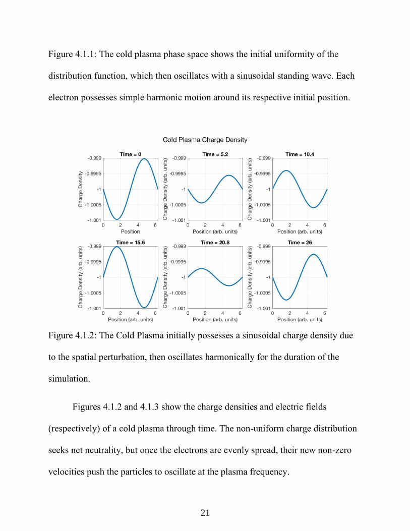
Figure 4.1.1: The cold plasma phase space shows the initial uniformity of the

distribution function, which then oscillates with a sinusoidal standing wave. Each

electron possesses simple harmonic motion around its respective initial position.

Figure 4.1.2: The Cold Plasma initially possesses a sinusoidal charge density due

to the spatial perturbation, then oscillates harmonically for the duration of the

simulation.

Figures 4.1.2 and 4.1.3 show the charge densities and electric fields

(respectively) of a cold plasma through time. The non-uniform charge distribution

seeks net neutrality, but once the electrons are evenly spread, their new non-zero

velocities push the particles to oscillate at the plasma frequency.

22

Figure 4.1.3: The electric field oscillation behaves similar to the charge density

oscillation, as the electrostatic model means that the electric field is merely the

negative of the charge density’s derivative in space.

Figure 4.1.4 shows the time evolution of the kinetic, electric potential, and

total energies. Each energy is found using Equations 3.3.1, 3.3.2, and the sum of

the two equations, respectively. At t = 0, the energy is stored entirely in the form of

electric potential, since all particles possess velocities of zero. After the electrons

are displaced from equilibrium, kinetic energy grows and exchanges with electric

potential at a period dependent on 𝜔𝑝.

23

Figure 4.1.4: Cold Plasma Energies show a periodic exchange between the kinetic

and potential energies, tracking the total energy demonstrates the non-conserving

property of this simulation.

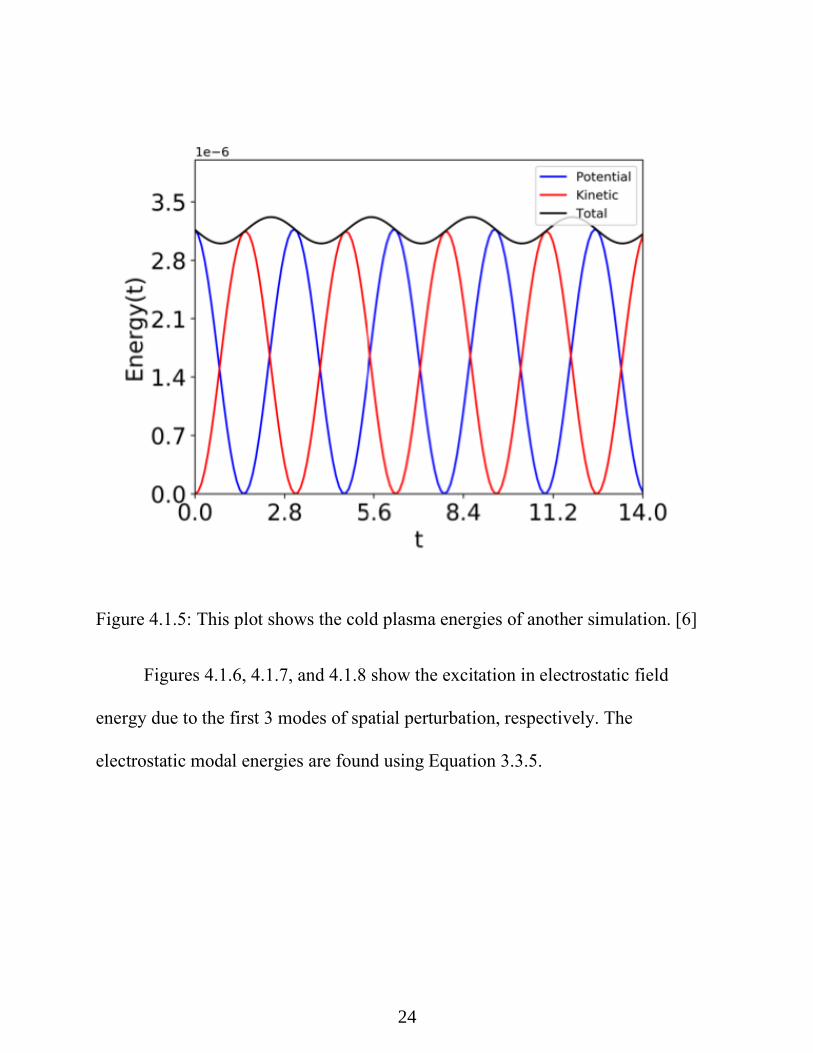
Figure 4.1.5 is taken from another paper using the kinetic PIC method to

model a cold plasma. [6] Comparing with Figure 4.1.4, the two plots possess the

same shape, although the magnitudes differ due to different initial plasma

parameters.

24

Figure 4.1.5: This plot shows the cold plasma energies of another simulation. [6]

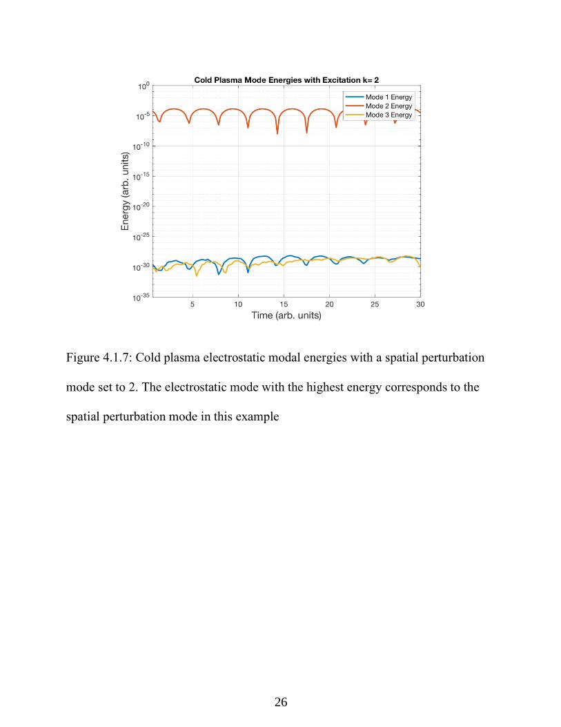
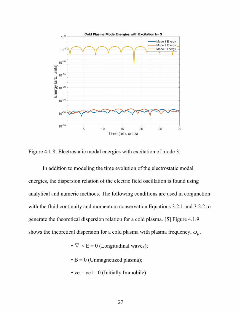
Figures 4.1.6, 4.1.7, and 4.1.8 show the excitation in electrostatic field

energy due to the first 3 modes of spatial perturbation, respectively. The

electrostatic modal energies are found using Equation 3.3.5.

25

Figure 4.1.6: With an initial spatial perturbation mode set to 1, the modal

electrostatic energies of the cold oscillation are found using Equation 3.3.5 [2]

The initially defined mode of spatial perturbation causes an excitation in the

electrostatic energy corresponding with the same wavelength. This modal

correspondence is confirmed with the electrostatic modal energy being highest

when compared to the other modes. This correspondence between the spatial

perturbation and electrostatic modal energies can be seen in Figures 4.1.7 and

4.1.8, where two more simulations were run with identical parameters, only

differing by the initial spatial perturbation.

26

Figure 4.1.7: Cold plasma electrostatic modal energies with a spatial perturbation

mode set to 2. The electrostatic mode with the highest energy corresponds to the

spatial perturbation mode in this example

27

Figure 4.1.8: Electrostatic modal energies with excitation of mode 3.

In addition to modeling the time evolution of the electrostatic modal

energies, the dispersion relation of the electric field oscillation is found using

analytical and numeric methods. The following conditions are used in conjunction

with the fluid continuity and momentum conservation Equations 3.2.1 and 3.2.2 to

generate the theoretical dispersion relation for a cold plasma. [5] Figure 4.1.9

shows the theoretical dispersion for a cold plasma with plasma frequency, 𝜔𝑝.

• ∇ × E = 0 (Longitudinal waves);

• B = 0 (Unmagnetized plasma);

• ve = ve1= 0 (Initially Immobile)

28

Figure 4.1.9: Theoretical dispersion relation for a cold plasma, found analytically

using the fluid continuity and momentum conservation equations combined with

the conditions of a cold plasma. [2]

Figures 4.1.10 to 4.1.14 show the dispersion relation for a cold plasma with

plasma frequencies 𝜔𝑝 and modes of excitation. These plots agree well with the

theoretical relation 𝜔 = 𝜔𝑝. Comparing to Figure 4.1.9, the group velocities are all

𝑣𝑔 =𝑑𝜔

𝑑𝑘= 0, since these are standing waves and do not propagate. Figure 4.1.11 is

taken from another paper for comparison. [6] The disagreement between the

theoretical and numeric dispersion in this other paper’s simulation may be due to

the chosen parameters. The parameters chosen were 2048 particles, 256 grid, a 4π

grid length points, 150 time steps, a dt = 0.1, with a sinusoidal spatial perturbation

of 0.001 of amplitude.

29

Figure 4.1.10: Cold plasma numerical dispersion relation with 𝜔𝑝=1 and spatial

perturbation mode=1.

30

Figure 4.1.11: This numerical dispersion plot is taken from another PIC simulation.

The disagreement between the theoretical black line and Fourier amplitudes may

be be due to the chosen parameters. [6]

31

Figure 4.1.12: Cold plasma numerical dispersion relation with 𝜔𝑝=2 and spatial

perturbation mode=1.

Figure 4.1.13: Cold plasma numerical dispersion relation with 𝜔𝑝=2 and spatial

perturbation mode=2

32

Figure 4.1.14: Cold plasma numerical dispersion relation with 𝜔𝑝=3 and mode=2.

Figures 4.1.10, 4.1.12, and 4.1.14 show the same cold plasma simulation

only differing in 𝜔𝑝 and the mode of spatial perturbation. Altering 𝜔𝑝 changes the

temporal rate of harmonic oscillation, whereas altering the mode of spatial

perturbation changes the wavelength of oscillation. 𝜔𝑝 affects the computer

defined parameters of charge q and mass m, which in turn effect the force acting on

the particles. The force defines the motion of the particles, which then in turn

dictate the electric fields, as the position of each particle determines the spatial

charge densities.

33

4.2 Electron Plasma Waves

Figure 4.2.1: Theoretical dispersion relation for electron plasma waves [3]

The plot above shows the theoretical dispersion relation for electron plasma

waves. Electron plasma waves are among the most fundamental phenomenon in

plasma physics. These waves are electrostatic in nature and propagate in

unmagnetized plasmas. They are high frequency waves and the ions are treated as

approximately unperturbed. The characteristics associated with Electron Plasma

Waves are as follows:

• ∇ × E = 0 (Longitudinal waves);

• B = 0 (Unmagnetized plasma);

• ve = ve1 ∥ E

Given the assumption of fixed ions, generating the dispersion relation only

requires solving electron continuity and momentum equations and Poisson’s

34

equation. The resulting electric field dispersion relation is represented by the

following equation. [5]

𝜔2 = 𝜔𝑝2 + 3𝑣𝑡ℎ

2 𝑘2 (4.2.1)

Where 𝑣𝑡ℎ2 is the Maxwellian thermal velocity of the electrons. Spatial input

variable are defined as follows: 𝐿=50, 𝑛𝑡=800, 𝑑𝑡= 0.0999/2, 𝑛𝑔=500. The species

input variables are defined as: 𝑁 =32,000, 𝑞𝑚 = −0.01, 𝑣𝑡1 = 1, 𝑣0 =0. [5] Figures

4.2.2, 4.2.4, and 4.2.5 were all created with 𝑣𝑡1 = 1, producing an initial

distribution function with a “hot” Maxwellian velocity distribution.

The following plots show a correspondence between the theoretical

dispersion curve and the Fourier amplitudes of the electric field data. Although the

plots do not show as much agreement as Figure 4.2.3 (taken from another paper),

the parabolic curve of the theoretical dispersion relation is suggested in the

numerical Fourier amplitudes.

35

Figures 4.2.2: Numerical dispersion relation of electron plasma waves of 𝜔𝑝=1

with theoretical curve for comparison.

Figure 4.2.3: Numerical dispersion relation of electron plasma waves. [5]

36

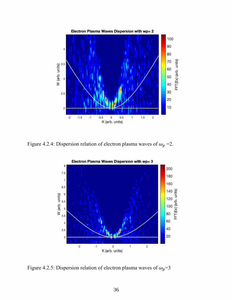
Figure 4.2.4: Dispersion relation of electron plasma waves of 𝜔𝑝 =2.

Figure 4.2.5: Dispersion relation of electron plasma waves of 𝜔𝑝=3

37

4.3 Two-Stream Instability

An instability consisting of counter-streaming electrons was modeled by

defining each stream with opposing initial drift velocities, 𝑣0. Since the initial

velocities are single valued, the initial distribution may be considered as “cold”.

Spatial input variables were defined: 𝐿=2𝜋, 𝑛𝑠𝑝=2, 𝑛𝑡=300, 𝑑𝑡=0.2, 𝑛𝑔=32.

Species input variables (both streams): 𝑁 = 128, 𝑤𝑝 = 1, 𝑞𝑚 = −1, and 𝑣0 =±1

Both streams were given perturbation settings of 𝑚𝑜𝑑𝑒=1, 𝑥1=0.001. All other

parameters were set to zero.

Figure 4.3.1: Phase-space time evolution of two-stream instability.

38

Figure 4.3.1 shows the phase-space evolution of the two streams. From the

initial time t = 0 to approximately t = 15, there is linear behavior in the growth of

the perturbation. After the maximum electric field is reached, nonlinear behavior

develops as the electron streams become thermalized.

Figure 4.3.2: Two-stream time evolution of charge density.

39

Figure 4.3.3: Two-stream electric field time evolution.

Figures 4.3.2 and 4.3.3 show the charge density and electric field evolution

of the two streams. Figure 11-4 shows the kinetic, electric potential, and total

energy. The electric field growth coincides with a drop in kinetic energy in both

streams. It should be noted that each stream possesses identical kinetic energies in

time; since the distributions are symmetric in phase space.

40

Figure 4.3.4: Two-stream kinetic, electric potential, and total energies.

The figure above shows the kinetic, electric potential, and total energies.

Exponential growth of electric potential energy in first phase of time evolution can

be seen. The electric field growth coincides with a drop in kinetic energy in both

streams. It should be noted that each stream possesses identical kinetic energies in

time; since the distributions are symmetric in phase space.

41

Figure 4.3.5: Time evolution of the electrostatic modal energies, with most

of the energy in the excited mode 1 until the instability reaches maximum electric

field. After this point in time the streams become thermalized and the other modes

developed comparable energies.

42

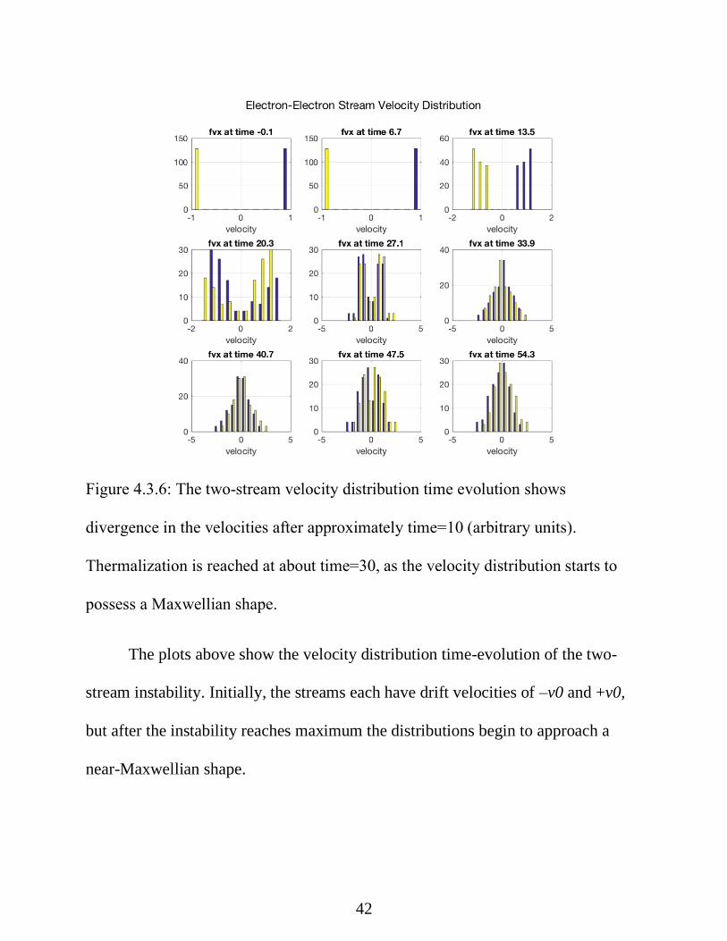
Figure 4.3.6: The two-stream velocity distribution time evolution shows

divergence in the velocities after approximately time=10 (arbitrary units).

Thermalization is reached at about time=30, as the velocity distribution starts to

possess a Maxwellian shape.

The plots above show the velocity distribution time-evolution of the two-

stream instability. Initially, the streams each have drift velocities of –v0 and +v0,

but after the instability reaches maximum the distributions begin to approach a

near-Maxwellian shape.

43

Figure 4.3.7: Drift energies for each electron stream. Both streams possess

identical energies for each case. The drift energies initially hold at a steady value,

until maximum instability, when the thermal energy takes over.

44

Figure 4.3.8: Time evolution of the thermal energies of each steam show identical

behavior between the two streams. During the exponential increase in electric field,

the velocities start to become thermalized simultaneously.

45

4.4 Landau Damping

As opposed to a cold plasma, a thermal plasma possesses a Maxwellian

velocity distribution. Even though the electrons are assumed to be collisionless, the

electrons gain kinetic energy and the electric field amplitude decays in time. When

individual electrons move in the electric field, they can diminish their energy

(electron velocity larger than phase velocity of wave) or receive additional energy

from the wave (electron velocity less than phase velocity of wave). The energy

balance for a swarm of electrons depends on the quantity of “cold” and “hot”

electrons. For a Maxwellian distribution, the quantity of “cold” electrons with a

velocity of zero is more than quantity of “hot” electrons. This leads to the damping

of the electric field perturbation. [2]

Spatial input variable are defined for this example: 𝐿=2𝜋, 𝑛𝑡=300, 𝑑𝑡=0.1,

𝑛𝑔=256. The species input variables of 𝑁 =8192, 𝑤𝑝 = 1, 𝑤𝑐 = 0, 𝑞𝑚 = −1, 𝑣𝑡1 =

0.5, 𝑣0 =0. A spatial perturbation was given with 𝑚𝑜𝑑𝑒=1, 𝑥1=0.02. Figure 12-1

shows the initial phase space, with a Maxwellian distribution with a mean velocity

of zero.

Figures 13-2 and 13-3 show the time evolution of the charge density and

electric field. Initially the electric field has a smooth sinusoidal shape, but overtime

flattens due to Landau damping.

46

Figure 4.4.1: Initial distribution function represented in phase space. As opposed to

the cold plasma and two-stream examples, and similar to the electron plasma

waves, the electrons are given an initial Maxwellian velocity distribution.

47

Figure 4.4.2: Looking at the charge density evolution, the initially rough sinusoidal

shape quickly decays and loses coherence due to Landau damping.

48

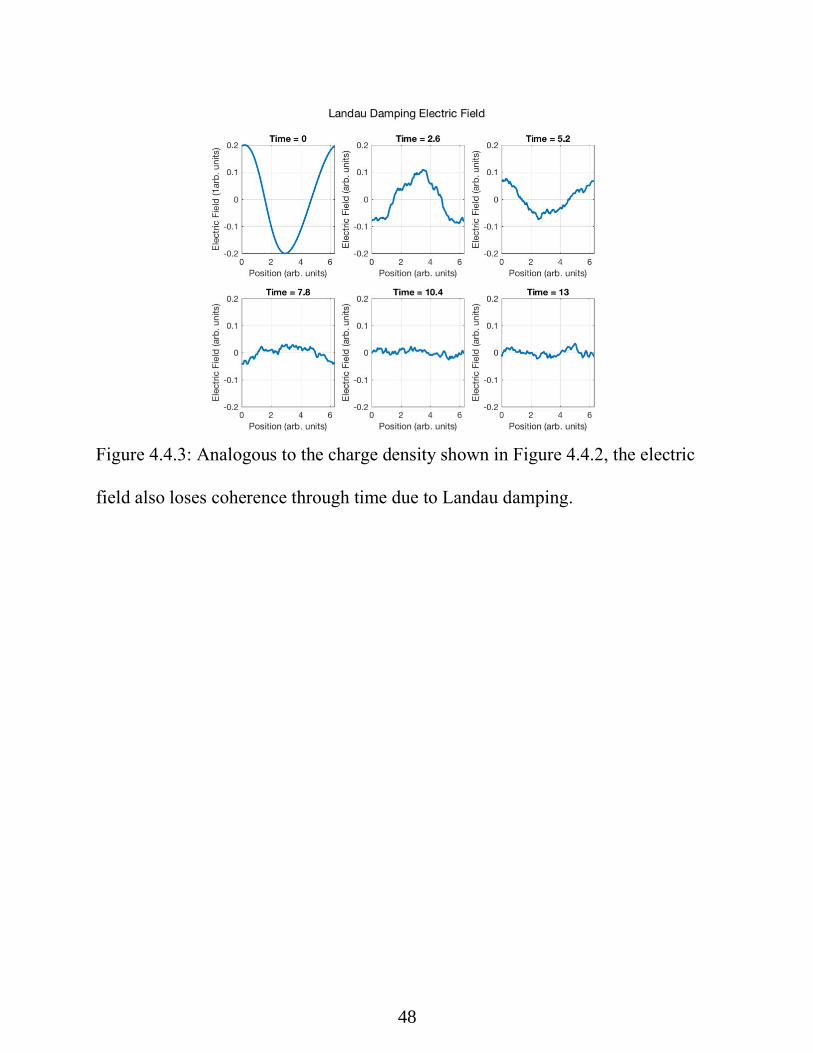
Figure 4.4.3: Analogous to the charge density shown in Figure 4.4.2, the electric

field also loses coherence through time due to Landau damping.

49

Figure 4.4.4: The time evolution of the velocity distribution shows how the

Maxwellian shape is virtually unchanged while the electric field decays.

50

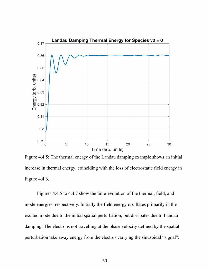
Figure 4.4.5: The thermal energy of the Landau damping example shows an initial

increase in thermal energy, coinciding with the loss of electrostatic field energy in

Figure 4.4.6.

Figures 4.4.5 to 4.4.7 show the time-evolution of the thermal, field, and

mode energies, respectively. Initially the field energy oscillates primarily in the

excited mode due to the initial spatial perturbation, but dissipates due to Landau

damping. The electrons not travelling at the phase velocity defined by the spatial

perturbation take away energy from the electros carrying the sinusoidal “signal”.

51

Figure 4.4.6: The electrostatic field energy shows an exponentially decaying

oscillation, characteristic of Landau Damping of the electric field.

52

Figure 4.4.7: Landau damping presented in multiple electrostatic field energy

modes. The initial spatial perturbation in the particle positions gives mode 1 the

maximum energy. After approximately time=10, however, the second and third

modes possess comparable energies. This spreading of electrostatic energy

between the modes in an indication of thermalization in the electron velocities.

53

4.5 Beam-Plasma

Like a two-stream instability, a beam-plasma consists of two “cold” species.

The beam consists of stationary ions, while the plasma is made of mobile electrons

with a drift velocity. Separate parameters are defined for each species: charge-to-

mass 𝑞𝑚 and number of particles, N. Spatial input variables were provided,

𝐿=2𝜋, 𝑛𝑠𝑝=2, 𝑛𝑡=1200, 𝑑𝑡=0.2, 𝑛𝑔=64. Species input variables of 𝑁 = 512, 64,

𝑤𝑝 = 0.03, 1, 𝑞𝑚 = -1, 0.001, 𝑣0 =1, 0, respectfully for electrons and ions. A

spatial electron perturbation was defined: 𝑚𝑜𝑑𝑒=1, 𝑥1=0.01. All other simulation

parameters are set to zero.

Figure 4.5.1 shows the beam-plasma phase space evolution. Giving an initial

spatial perturbation to the plasma causes an instability to grow, similar to the two-

stream example. During the linear phase of growth, the spatial and electric field

perturbation (and therefore electric field) in the electron plasma grows

exponentially in time.

54

Figure 4.5.1: The beam-plasma phase space shows a similar behavior as the two-

stream example. The blue dots represent mobile electrons with an initial drift

velocity of 1. The red dots represent ions with a much lower charge-mass ratio.

55

Figure 4.5.2: The beam-plasma electric field time evolution shows a mostly

sinusoidal shape, as the electrons are the primary factor in electric field. Electrons

are much higher in number and have a much higher plasma frequency, the

computer parameter which determines charge and mass when combined with the

charge-mass ratio.

Figure 4.5.2: The Beam Plasma simulation shows the exponential growth

and subsequent oscillation after saturation in electric field energy. Figure 13-4

shows the modes of electric field energy.

56

Figure 4.5.3: Similar to the two-stream, the electrostatic field energy increases

exponentially until about time=110. After this time, the field energy starts to

oscillate, exchanging primarily with the electrons’ kinetic energy.

57

Figure 4.5.4: The modal electrostatic field energies show that the first mode is

dominant, as the electrons are spatially perturbed to excite that wavelength.

58

Figure 4.5.5: The time evolution of the beam-plasma velocity distribution shows

that the he heavy ions maintain their velocities much more than the electron

plasma, which starts to develop a Maxwellian distribution near the end of the run.

Figures 4.5.6, 4.5.7, and 4.5.8 show the thermal, drift, and kinetic energies

of each species, respectively. The exponential growth in electric field coincides

with growth in both species’ thermal energies, although the increase is more

significant in the stationary ions.

59

Figure 4.5.6: The thermal energies of both the electrons and ions increase

exponentially, coinciding with the increase in electric field.

60

Figure 4.5.7: These plots show the evolution of the drift energies in each species.

The electrons lose some drift energy due to thermalization, although almost all the

kinetic energy still consists of drift energy. The ion beam gains some drift energy,

but is 12 orders of magnitude less than the gain in thermal energy in the species.

61

Figure 4.5.8: Most of the electrons’ kinetic energy consists of drift energy, as the

species is given an initial drift velocity. The rest of the electron kinetic energy is

thermal velocity, which can be seen in Figure 4.5.7. Most of the ions’ kinetic

energy consists of thermal energy, which can be seen in Figure 4.5.6.

62

Chapter 5: Summary

This work was initially intended to demonstrate a fully physical ionospheric

plasma system, but the difficulty of creating a complete model proved too

immense. Instead, the work became focused on how to translate FORTRAN and

Python code to MATLAB, and how to guarantee the accuracy of the generated

output by comparison with the original code. In addition to the calculation of the

electric field acting on each particle, a more physically complete simulation

requires other physical considerations. The magnetic fields as well as particle

collisions of each particle must be added to the computational toolkit to generate a

more complete set of plasma interactions. [2].

Relative to a computational fluid dynamic approach to plasma, a particle-in-

cell approach is more computationally taxing. Despite the computational cost,

however, useful plasma phenomenon is representable with PIC. This work

ultimately consists of demonstrating the relatively elementary wave properties of a

cold stream, electron plasma waves, two-stream, Landau Damping, and electron-

beam systems. Comparing with expected theoretical results derived from the fluid

continuity and momentum equations as well as other physics, agreement was

obtained using the PIC method.

63

Bibliography

[1] Goldston, R.J.; Rutherford, P.H. (1995). Introduction to Plasma Physics. Taylor &

Francis. p. 1−2. ISBN 978-0-7503-0183-1.

[2] Birdsall, Charles K., and Allan B. Langdon. Plasma Physics via Computer Simulation.

IOP Publ., 2000.

[3] Chen, Francis F. Introduction to Plasma Physics and Controlled Fusion. Springer, 2018.

[4] R. Fonseca. Zpic - educational particle-in- cell code suite, accessed November 2020.

URL https://github.com/zambzamb/zpic.

[5] Calado, Rui. Computational Toolkit for Plasma Physics Education, 2018,

fenix.tecnico.ulisboa.pt/downloadFile/1970719973967420/ExtendedAbstract.pdf.

[6] Blandón, J S, et al. “Electrostatic Plasma Simulation by Particle-In-Cell Method Using

ANACONDA Package.” Journal of Physics: Conference Series, vol. 850, 2017, p.

012007., doi:10.1088/1742-6596/850/1/012007.

[7] Martin, Daniel. Electrostatic PIC Simulation of Plasmas in One Dimension, 2007,

porl2.tripod.com/sitebuildercontent/sitebuilderfiles/dmreport1.pdf.

[8] H. Matsumoto, Y. Omura, Particle simulations of electromagnetic waves and its

applications to space plasmas, in: H. Matsumoto, T. Sato (Eds.), Computer Simulations

of Space Plasmas, Terra Pub. and Reidel Co., 1984, pp. 43–102.

[10] Shapiro, V. D., et al. “Lower Hybrid Dissipative Cavitons and Ion Heating in the

Auroral Ionosphere.” Physics of Plasmas, vol. 2, no. 2, 1995, pp. 516–526.,

doi:10.1063/1.870976.

64

[11] Vahedi, V., & Surendra, M. (1995). A Monte Carlo collision model for the particle-in-

cell method: applications to argon and oxygen discharges. Computer Physics

Communications, 87(1–2), 179–198.

[12] BIRDSALL, C. (n.d.). Particle-In-Cell Charged-Particle Simulations, Plus Monte-Carlo

Collisions with Neutral Atoms, Pic-Mcc. IEEE TRANSACTIONS ON PLASMA

SCIENCE, 19(2), 65–85.

[13] The Plasma Theory and Simulation Group, 2008, ptsg.egr.msu.edu/.

[14] Layers of the Ionosphere.

www.google.com/imgres?imgurl=https%3A%2F%2Fcdn.britannica.com%2F46%2F109

746-050-9511BBEF%2Fdifferences-layers-ionosphere-

Earth.jpg&imgrefurl=https%3A%2F%2Fwww.britannica.com%2Fscience%2FF-

region&tbnid=L0SaQkv2MgDN8M&vet=12ahUKEwiopov10KntAhWVFqwKHcfgDm

wQMygEegUIARDaAQ..i&docid=HpeEiTcYyKNkpM&w=1600&h=934&q=ionospher

e&ved=2ahUKEwiopov10KntAhWVFqwKHcfgDmwQMygEegUIARDaAQ.

65

Appendix %ES1 - Main Program Code By Richard Vanderburgh at Wright State

University 2020

clear variables

close all

clc

FIRST_EE

INIT

t=0;

SETRHO

FIELDS

dxdt = dx/dt;

%{

axis tight manual % this ensures that getframe() returns a

consistent size

v = VideoWriter(sprintf(example));

open(v);

%}

for t=1:nt

if mod(t,ixvx)==0|| t==1 && ixvx~=0

if t==1

phasecounter=1;

PhaseSpacePlots=figure;

hold on

end

for species=1:nsp

set(0,'CurrentFigure',PhaseSpacePlots)

h1=subplot(3,3,phasecounter) ;

%subplot(2,2,1)

scatter(x(:,species)/dxi,vx(:,species)*dxdt, '.');

%set(gca,'FontSize',12)

grid on

ylim([-3 3]);

xlim([0 L]);

hold on

end

hold on

if t==1

title(['Time = ',num2str((t-1)*dt-dt/2),]);

66

xlabel('Position (arb. units)');

ylabel('Velocity (arb. units)');

elseif t ~= 1

title(['Time = ',num2str((t)*dt-dt/2),]);

xlabel('Position (arb. units)');

ylabel('Velocity (arb. units)');

end

phasecounter=phasecounter+1;

hold off

drawnow

%frame = getframe(gcf);

%writeVideo(v,frame);

end

if t==nt && ixvx~=0

set(0,'CurrentFigure',PhaseSpacePlots)

suptitle([sprintf(example), 'Phase Space'])

saveas(PhaseSpacePlots,[sprintf(example), 'PhaseSpace.png'])

end

if t==1

SETV

end

ACCEL

MOVE

FIELDS

for species=1:nsp

te(t,1)=te(t,1)+ke(t,species);

end

te(t,1)=te(t,1)+EnergiaP(t,1);

if mod(t,irho)==0|| t==1 && irho~=0;

if t==1

rhocounter=1;

ChargeDensityPlots=figure;

hold on

end

set(0,'CurrentFigure',ChargeDensityPlots)

h2=subplot(3,3,rhocounter) ;

%subplot(2,2,2)

plot(gridx,real(rho),'LineWidth',2)

xlim([0 L]);

ylim([-4 -0]);

grid on

hold on

xlabel('Position');

67

ylabel('Charge Density');

if t ==1

title(['Time = ',num2str((t-1)*dt)]);

elseif t ~= 1

title(['Time = ',num2str((t)*dt)]);

xlabel('Position (arb. units)');

ylabel('Charge Density (arb. units)');

grid on

end

rhocounter=rhocounter+1;

drawnow

%hold off

end

if t==nt && irho~=0

set(0,'CurrentFigure',ChargeDensityPlots)

suptitle([sprintf(example), 'Charge Density'])

saveas(ChargeDensityPlots,[sprintf(example),

'ChargeDensity.png'])

end

%}

for species=1:nsp

% Clear out old charge density.

for j = 2:ng+1

rho(j) = rho0;

end

rho(1) = 0;

end

if mod(t,iphi)==0 || t==1 && iphi~=0

if t==1

phicounter=1;

PotentialPlots=figure;

hold on

end

set(0,'CurrentFigure',PotentialPlots)

h3=subplot(3,3,phicounter) ;

%subplot(2,2,3)

plot(gridx,real(phi),'LineWidth',2)

xlim([0 L]);

%ylim([-3 -1]);

grid on

%hold on

xlabel('Position (arb. units)');

68

ylabel('Potential (1arb. units)');

if t ==1

title(['Time = ',num2str((t-1)*dt)]);

elseif t ~= 1

title(['Time = ',num2str((t)*dt)]);

xlabel('Position (arb. units)');

ylabel('Potential (arb. units)');

grid on

end

drawnow

phicounter=phicounter+1;

hold off

end

if t==nt && iphi~=0

set(0,'CurrentFigure',PotentialPlots)

suptitle([sprintf(example), 'Electric Potential'])

saveas(PotentialPlots,[sprintf(example),

'ElectricPotential.png'])

end

if mod(t,iE)==0 || t==1 && iE~=0

if t==1

Ecounter=1;

ElectricFieldPlots=figure;

hold on

end

set(0,'CurrentFigure',ElectricFieldPlots)

h4=subplot(3,3,Ecounter) ;

%subplot(2,2,4)

plot(gridx,real(E(t,:)),'LineWidth',2)

xlim([0 L]);

ylim([-1 1]);

grid on

%hold on

xlabel('Position (arb. units)');

ylabel('Electric Field (1arb. units)');

if t ==1

title(['Time = ',num2str((t-1)*dt)]);

elseif t ~= 1

title(['Time = ',num2str((t)*dt)]);

xlabel('Position (arb. units)');

ylabel('Electric Field (arb. units)');

grid on

end

69

Ecounter=Ecounter+1;

drawnow

hold off

end

if t==nt && iE~=0

set(0,'CurrentFigure',ElectricFieldPlots)

suptitle([sprintf(example), 'Electric Field'])

saveas(ElectricFieldPlots,[sprintf(example),

'ElectricField.png'])

end

if mod(t,ifvx)==0 || t==1 && ifvx~=0

if t==1

fvxcounter=1;

fvxPlots=figure;

hold on

end

set(0,'CurrentFigure',fvxPlots)

h5=subplot(3,3,fvxcounter) ;

hist(vx);

grid on

if t==1

title(['fvx at time ',num2str((t-1)*dt-dt/2),]);

xlabel('velocity');

elseif t ~= 1

title(['fvx at time ',num2str((t)*dt-dt/2),]);

xlabel('velocity');

%xlim([-3 3]);

%ylim([0 50]);

end

fvxcounter=fvxcounter+1;

drawnow

hold off

end

if t==nt && ifvx~=0

set(0,'CurrentFigure',fvxPlots)

suptitle([sprintf(example), 'Velocity Distribution'])

70

saveas(fvxPlots,[sprintf(example), 'Velocity

Distribution.png'])

end

%t*dt-dt/2

end

%suptitle([sprintf(example), 'Electric Field with wp= ',

num2str(wp(1)) ' and Mode= ' num2str(mode(1))])

%saveas(ElectricFieldPlots,[sprintf(example),

'ElectricField.png'])

%close(v);

%plotspectrnew

wk

PLOTTING

%End of Simulation :)