one to many distribution - edxmitx+ctl.sc1x_1+2... · one to many distribution . ... factors for...

MIT Center for Transportation & Logistics

CTL.SC1x -Supply Chain & Logistics Fundamentals

One to Many Distribution

CTL.SC1x - Supply Chain and Logistics Fundamentals Lesson: One to Many Distribution

How can I distribute products?

DC

One-to-One – direct or point to point movements from origin to destination

One-to-Many – multi-stop moves from a single origin to many destinations

DC

Many-to-Many – moving from multiple origins to multiple destinations usually with a hub or terminal

T DC

DC DC

2


Example: OfficeMin •  Your firm delivers office supplies to

firms within the I-95 highway loop around Boston from your distribution center located in Newton.

•  You want to estimate: 1.  Expected cost per day, 2.  Expected truck fleet size, and 3.  Sensitivity of the solution.

•  What information do I need? •  What methodology should I use?

3


Defining Delivery Districts

4


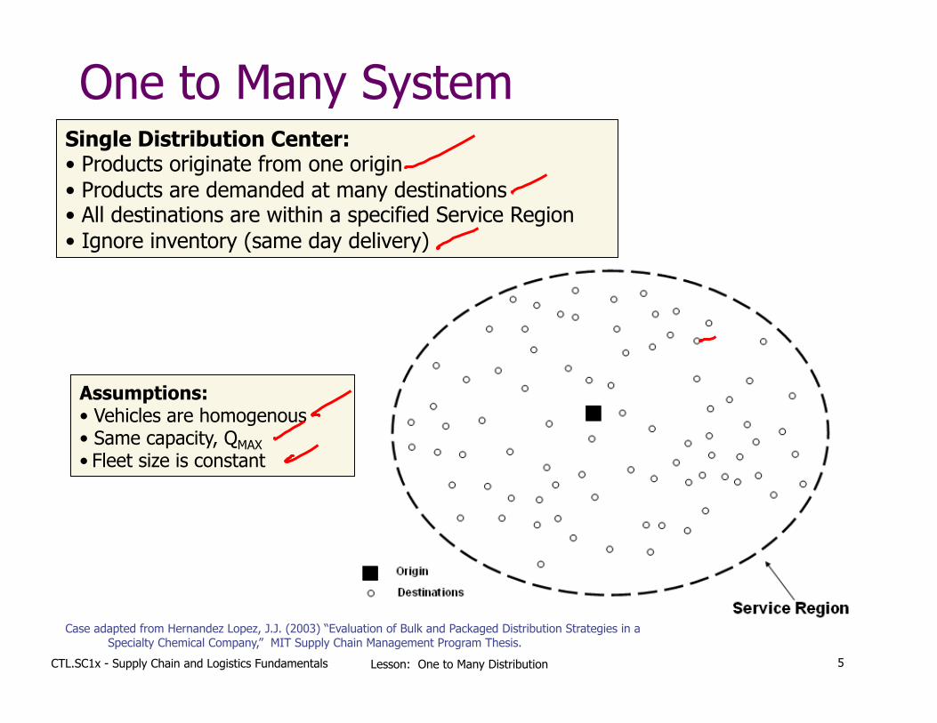
One to Many System Single Distribution Center: •  Products originate from one origin •  Products are demanded at many destinations •  All destinations are within a specified Service Region •  Ignore inventory (same day delivery)

Assumptions: •  Vehicles are homogenous •  Same capacity, QMAX •  Fleet size is constant

Case adapted from Hernandez Lopez, J.J. (2003) “Evaluation of Bulk and Packaged Distribution Strategies in a Specialty Chemical Company,” MIT Supply Chain Management Program Thesis.

5


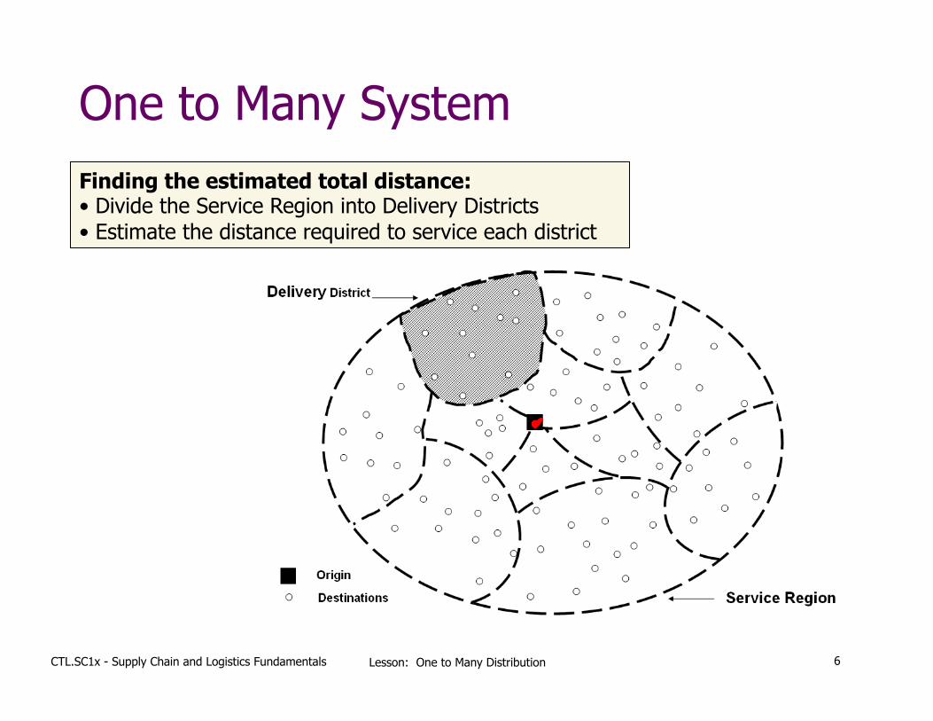
One to Many System Finding the estimated total distance: •  Divide the Service Region into Delivery Districts •  Estimate the distance required to service each district

6


One to Many System Route to serve a specific district: •  Line haul from origin to the 1st customer in the district •  Local delivery from 1st to last customer in the district •  Back haul (empty) from the last customer to the origin

2TOUR LineHaul Locald d d≈ +

dLineHaul = Distance from origin to center of gravity (centroid) of delivery district

dLocal = Local delivery between c customers in one district

How do we estimate distances? 1.  Point to Point 2.  Routing or within a Tour

7


Estimating Point to Point Distances

8


Distance Estimation: Point to Point •  Why bother?

•  How to do it?

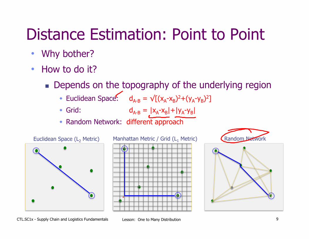
n  Depends on the topography of the underlying region w  Euclidean Space: dA-B = √[(xA-xB)2+(yA-yB)2]

w  Grid: dA-B = |xA-xB|+|yA-yB|

w  Random Network: different approach

Euclidean Space (L2 Metric) Manhattan Metric / Grid (L1 Metric) Random Network

9


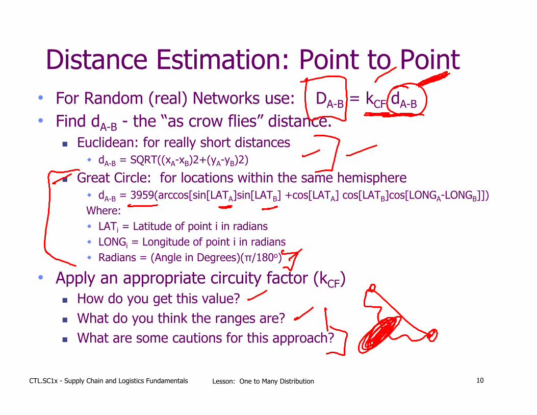
Distance Estimation: Point to Point •  For Random (real) Networks use: DA-B = kCF dA-B

•  Find dA-B - the “as crow flies” distance. n  Euclidean: for really short distances

w  dA-B = SQRT((xA-xB)2+(yA-yB)2)

n  Great Circle: for locations within the same hemisphere w  dA-B = 3959(arccos[sin[LATA]sin[LATB] +cos[LATA] cos[LATB]cos[LONGA-LONGB]]) Where: w  LATi = Latitude of point i in radians w  LONGi = Longitude of point i in radians w  Radians = (Angle in Degrees)(π/180o)

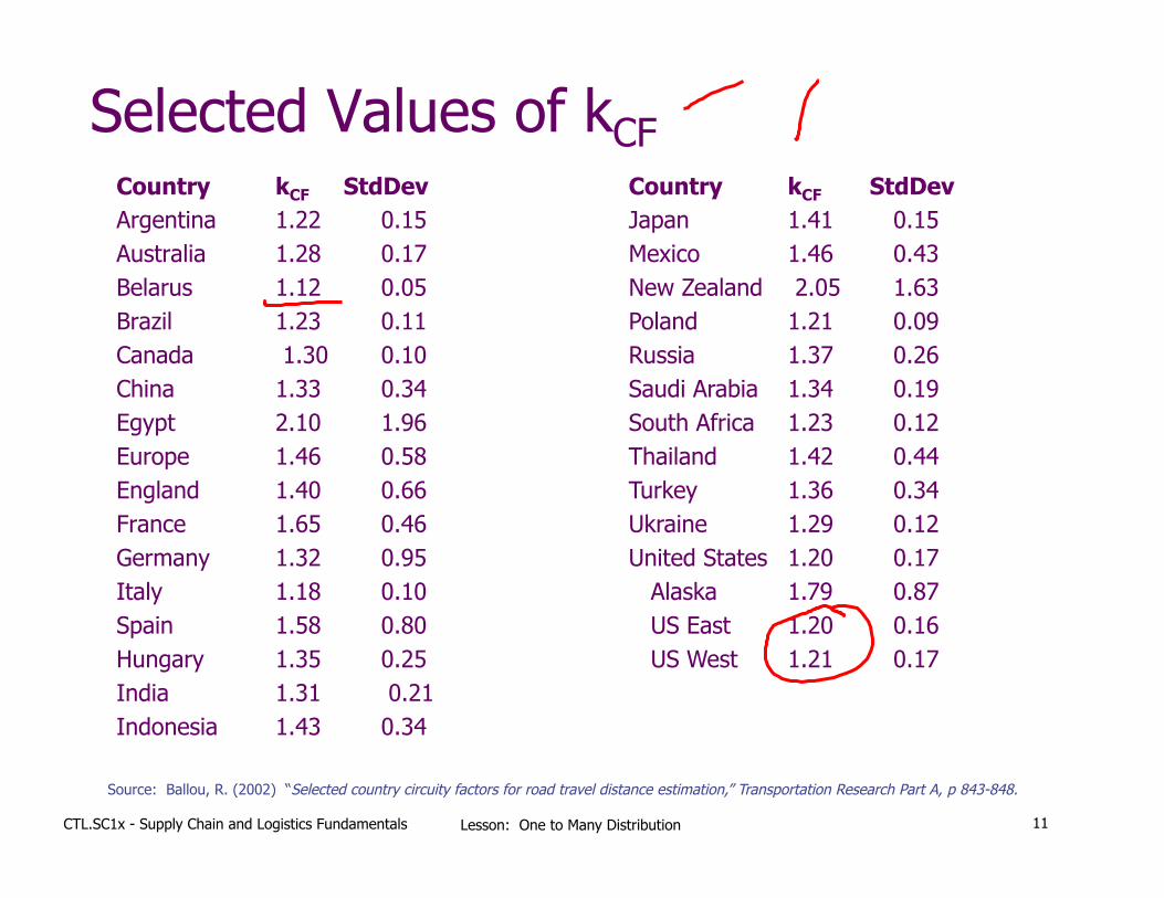
•  Apply an appropriate circuity factor (kCF) n  How do you get this value? n  What do you think the ranges are? n  What are some cautions for this approach?

10


Selected Values of kCF Country kCF StdDev Argentina 1.22 0.15 Australia 1.28 0.17 Belarus 1.12 0.05 Brazil 1.23 0.11 Canada 1.30 0.10 China 1.33 0.34 Egypt 2.10 1.96 Europe 1.46 0.58 England 1.40 0.66 France 1.65 0.46 Germany 1.32 0.95 Italy 1.18 0.10 Spain 1.58 0.80 Hungary 1.35 0.25 India 1.31 0.21 Indonesia 1.43 0.34

Country kCF StdDev Japan 1.41 0.15 Mexico 1.46 0.43 New Zealand 2.05 1.63 Poland 1.21 0.09 Russia 1.37 0.26 Saudi Arabia 1.34 0.19 South Africa 1.23 0.12 Thailand 1.42 0.44 Turkey 1.36 0.34 Ukraine 1.29 0.12 United States 1.20 0.17 Alaska 1.79 0.87 US East 1.20 0.16 US West 1.21 0.17

Source: Ballou, R. (2002) “Selected country circuity factors for road travel distance estimation,” Transportation Research Part A, p 843-848.

11


Estimating Route Distances

12


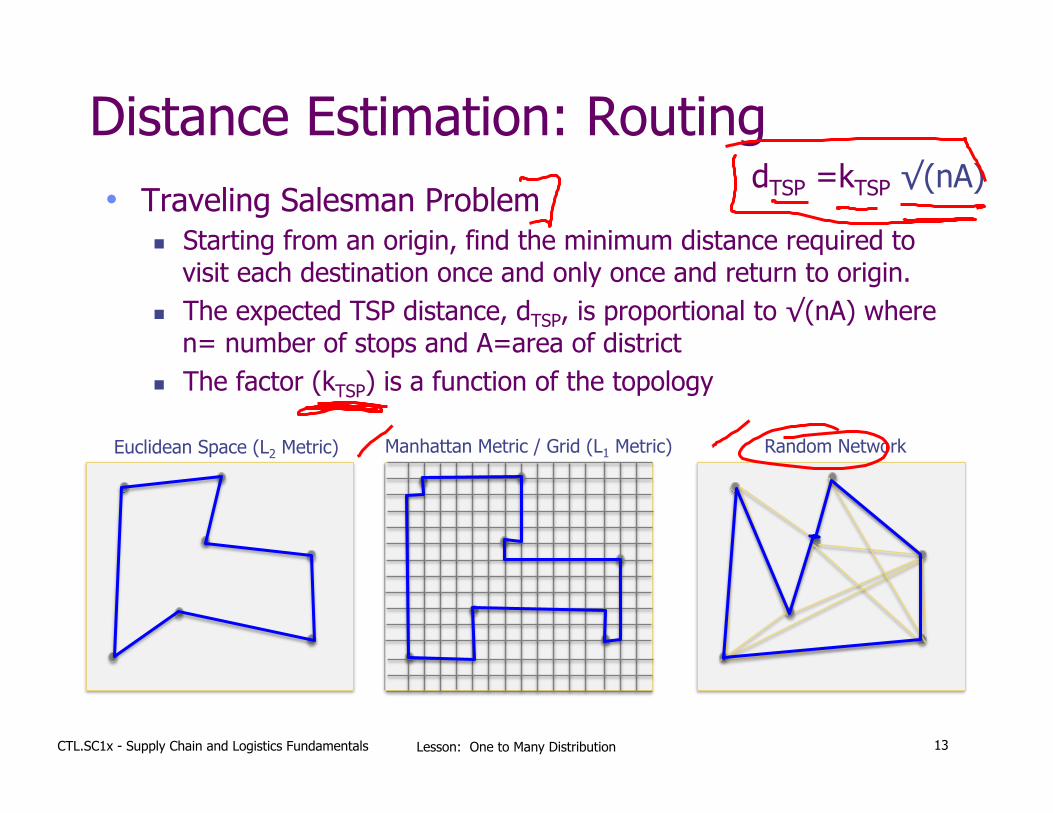
Distance Estimation: Routing •  Traveling Salesman Problem

n  Starting from an origin, find the minimum distance required to visit each destination once and only once and return to origin.

n  The expected TSP distance, dTSP, is proportional to √(nA) where n= number of stops and A=area of district

n  The factor (kTSP) is a function of the topology

Euclidean Space (L2 Metric) Manhattan Metric / Grid (L1 Metric) Random Network

13

dTSP =kTSP √(nA)


One to Many System •  What can we say about the expected

TSP distance to cover n stops in district with an area of A?

•  A good approximation, assuming a "fairly compact and fairly convex" area, is:

E dTSP!" #$ ≈ kTSP nA = kTSP n nδ

&

'()

*+ =kTSPnδ

A=Area of district n=Number of stops in district δ=Density (# stops/Area) k=VRP network factor (unitless) dTSP=Traveling Salesman Distance dstop=Average distance per stop

•  What values of kTSP should we use? –  Lots of research on this for L1 and L2 networks - depends on district shape,

approach to routing, etc. –  Euclidean (L2) Networks

•  kTSP = 0.57 to 0.99 depending on clustering & size of N (MAPE~4%, MPE~-1%) •  kTSP=0.765 commonly used

–  Grid (L1) Networks •  kTSP = 0.97 to 1.15 depending on clustering and partitioning of district

References: Daganzo, C.. (2010) Logistics Systems Analysis, 4th Edition Springer-Verlag. Larson, R. and Odoni, A. (1981) Urban Operations Research, http://web.mit.edu/urban_or_book/www/book/

14


Estimating Tour Distances

15


Estimating Tour Distance •  Finding the total distance traveled on all tours, where:

n  l = number of tours n  c = number of customer stops per tour and n  n=total number of stops = c*l

E dTOUR!" #$= 2dLineHaul +ckTSPδ

E dAllTours!" #$= lE dTOUR!" #$= 2ldLineHaul +nkTSPδ

•  Minimize number of tours by maximizing vehicle capacity

l = DQMAX

!

"#

$

%&

+

E dAllTours!" #$= 2DQMAX

!

"#

$

%&

+

dLineHaul +nkTSPδ

[x]+ = lowest integer value > x. This is a step function

Estimate this with continuous function: E([x]+ ) ~ E(x) + ½

16


Continuous Approximation

-

0.5

1.0

1.5

2.0

2.5

3.0

3.5

4.0

4.5

5.0

0 10 20 30 40 50 60 70 80

Num

ber

of T

ours

(D

/Qm

ax)

Values of Demand (D)

D/Qmax [D/Qmax]+ (D/Qmax)+1/2

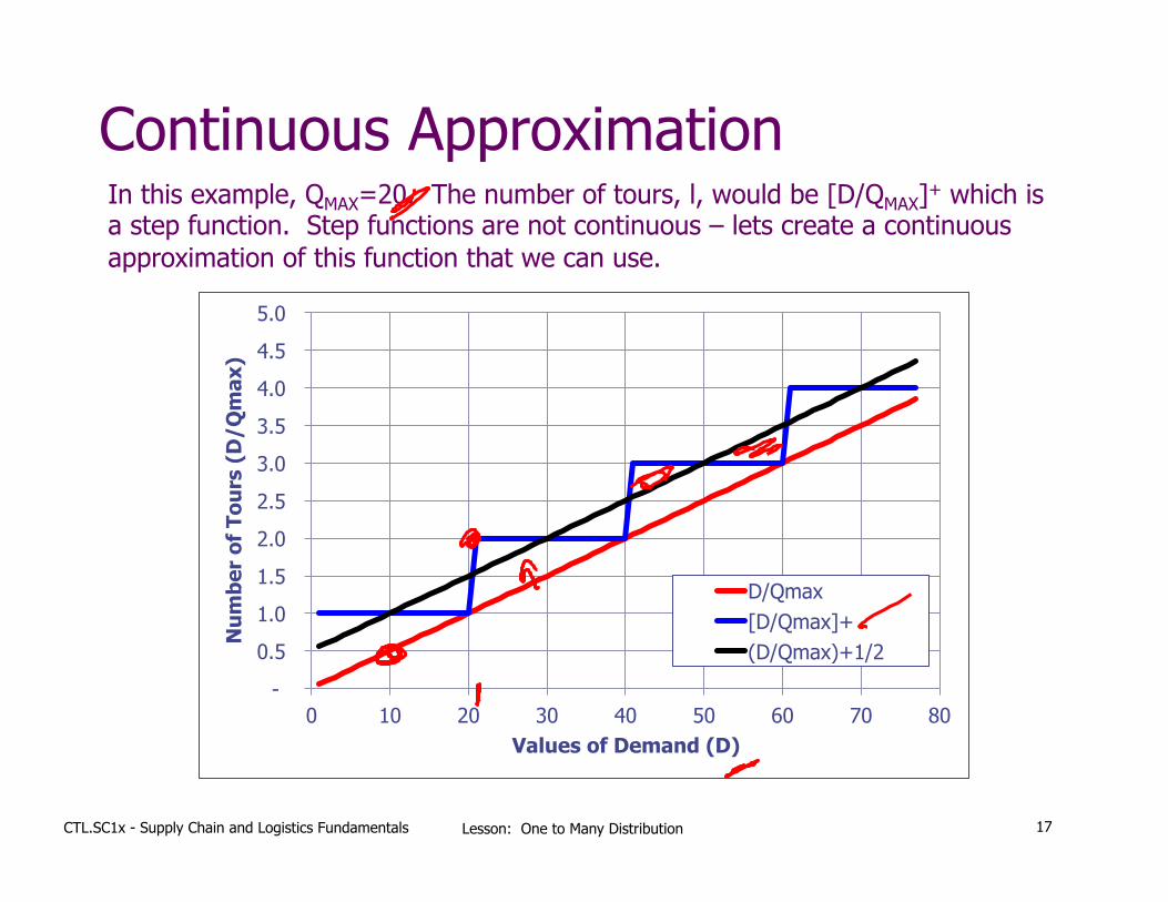
In this example, QMAX=20. The number of tours, l, would be [D/QMAX]+ which is a step function. Step functions are not continuous – lets create a continuous approximation of this function that we can use.

17


One to Many System

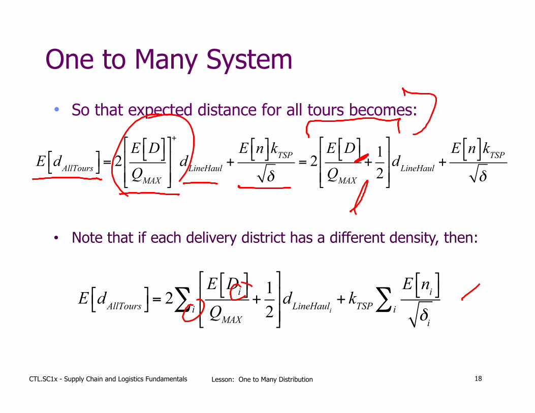
•  So that expected distance for all tours becomes:

•  Note that if each delivery district has a different density, then:

E dAllTours!" #$= 2E Di!" #$QMAX

+12

!

"%%

#

$&&dLineHaulii∑ + kTSP

E ni!" #$

δii∑

E dAllTours!" #$= 2E D!" #$QMAX

!

"##

$

%&&

+

dLineHaul +E n!" #$kTSP

δ= 2

E D!" #$QMAX

+12

!

"##

$

%&&dLineHaul +

E n!" #$kTSPδ

18


Putting it all together For identical districts, the approximate transportation cost to deliver to each customer becomes:

TransportCost = cs E n!" #$+E D!" #$QMAX

+12

!

"%%

#

$&&+ cd 2

E D!" #$QMAX

+12

!

"%%

#

$&&dLineHaul +

E n!" #$kTSPδ

'

(

))

*

+

,,+ cvsE D!" #$

Expected number of loads/unloads (customer + origin)

Expected number of linehaul moves or tours

Expected local delivery distance regardless of number of tours

Cost per item per stop

Expected distance for the linehaul portion. How do I get this?

E[n]=Expected number of stops in district E[D]=Expected demand in district QMAX=Capacity of each truck cs=Cost per stop ($/stop) cd=Cost per distance ($/mile) cvs=Cost per unit per stop ($/item-stop)

δ=Density (# stops/Area) kTSP =TSP network factor (unitless) dTSP=Traveling Salesman Distance dstop=Average distance per stop

19


Solution OfficeMin

20


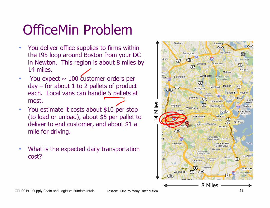
OfficeMin Problem •  You deliver office supplies to firms within

the I95 loop around Boston from your DC in Newton. This region is about 8 miles by 14 miles.

•  You expect ~ 100 customer orders per day – for about 1 to 2 pallets of product each. Local vans can handle 5 pallets at most.

•  You estimate it costs about $10 per stop (to load or unload), about $5 per pallet to deliver to end customer, and about $1 a mile for driving.

•  What is the expected daily transportation cost?

8 Miles

14 M

iles

21


OfficeMin

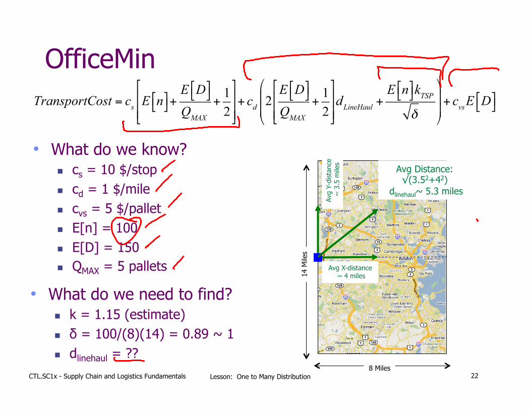
•  What do we know? n  cs = 10 $/stop n  cd = 1 $/mile n  cvs = 5 $/pallet n  E[n] = 100 n  E[D] = 150 n  QMAX = 5 pallets

22


+12

!

"%%

#

$&&+ cd 2

E D!" #$QMAX

+12

!

"%%

#

$&&dLineHaul +

E n!" #$kTSPδ

'

(

))

*

+

,,+ cvsE D!" #$

•  What do we need to find? n  k = 1.15 (estimate) n  δ = 100/(8)(14) = 0.89 ~ 1 n  dlinehaul = ??

8 Miles

14 M

iles

Avg X-distance ~ 4 miles

Avg

Y-di

stan

ce

~ 3

.5 m

iles

Avg Distance: √(3.52+42)

dlinehaul~ 5.3 miles


OfficeMin cs = 10 $/stop cd = 1 $/mile cvs = 5 $/pallet

23


+12

!

"%%

#

$&&+ cd 2

E D!" #$QMAX

+12

!

"%%

#

$&&dLineHaul +

E n!" #$kTSPδ

'

(

))

*

+

,,+ cvsE D!" #$

l =E D!" #$QMAX

+12=1505+ .5= 30.5

Estimated number of tours per day:

cs E n!" #$+ E l!" #$!"

#$=10 100+30.5( ) = $1305

Estimated stop (load/unload) cost per day:

cd 2E l!" #$dLineHaul +E n!" #$kTSP

δ

%

&

''

(

)

**=1 2(30.5)(5)+

100(1.15)1

%

&'

(

)*= 305+115= $420

Estimated distance (driving) cost per day:

cvsE D!" #$= 5(150) = $750Estimated stop-pallet costs per day:

Estimated total daily cost ~ $2400 to $2500

E[n] = 100 E[D] = 150 QMAX = 5 pallets

k = 1.15 δ = 1 dlinehaul = 5


Estimating Fleet Size [OPTIONAL – MORE ADVANCED]

24


Estimating the Fleet Size

W =dAllTourss

+ ltl + nts

•  Find minimum number of vehicles required based on the amount of required work time each day where n  M = minimum number of vehicles needed in fleet n  tw = available worktime for each vehicle per period n  W = required amount of work time each day n  s = average vehicle speed n  l = number of shipments per period n  tl = loading time per shipment n  ts = unloading time per stop

W =2dLineHauls

+ tl!

"#

$

%&E l'( )*+ E n'( )*

kTSPs δ

+ ts!

"#

$

%&

W =

2E l!" #$dLineHaul +E n!" #$kTSP

δ

%

&''

(

)**

s+ E l!" #$tl + E n!" #$ts

Mtw ≥W

25


W =2dLineHauls

+ tl!

"#

$

%&DQMAX

+12

'

()

*

+,+ n

kTSPs δ

+ ts!

"#

$

%&

Note that W is a linear combination of two random variables, n and D. But, they are not independent, in fact, D = nDc where Dc is the number of pallets per customer

a =2dLineHauls

+ tl!

"#

$

%&

1QMAX

'

()

*

+,= 0.144hrs

b =kTSPs δ

+ ts!

"#

$

%&= 0.525 hrs

c = 122dLinehauls

+ tl!

"#

$

%&= 0.361hrs

W = aD+bn+ cW = aDcn+bn+ cW = (aDc +b)n+ c

W = Xn+ cE[W ]= E[X ]E[n]+ cVar[W ]= E[n]Var[X ]+ E[X ]2Var[n]

Setting X=aDc+b, W is now a function of random variables, X and n.

Fleet Size tw = 10 hrs s = 45 mph tl = 0.5 hr ts = 0.5 hr

cs = 10 $/stop cd = 1 $/mile cvs = 5 $/pallet


k = 1.15 δ = 1 dlinehaul = 5

E Dc!" #$=1.5

Var[Dc ]=xi − x( )

2

i=1

n∑

n= 0.25

26


W = (aDc +b)n+ c = 0.144Dc +0.525( )n+0.361= Xn+ c

Fleet Size

W =2dLineHauls

+ tl!

"#

$

%&DQMAX

+12

'

()

*

+,+ n

kTSPs δ

+ ts!

"#

$

%&

E[n]=100 customersVar[n]= 400 (assumeσ n = 20)

tw = 10 hrs s = 45 mph tl = 0.5 hr ts = 0.5 hr

cs = 10 $/stop cd = 1 $/mile cvs = 5 $/pallet


k = 1.15 δ = 1 dlinehaul = 5

a = 0.144hrsb = 0.525 hrsc = 0.361hrs

E[W ]= E X!" #$E n!" #$+ c

E[W ]= (0.741)(100)+0.361= 74.46

E X!" #$= aE Dc!" #$+b = 0.144(1.5)+0.525= 0.741

Var[X ]= a2Var[Dc ]= 0.021(0.25) = 0.00525

E[Dc ]=1.5 palletsVar[Dc ]= 0.25

Var[W ]= E n!" #$Var X!" #$+ E X!" #$2Var n!" #$

Var[W ]= (100)(0.00525)+ (0.741)2(400) = 220

Distribution of required daily work hours:

µW ~ 75 hrs σW ~ 15 hrs


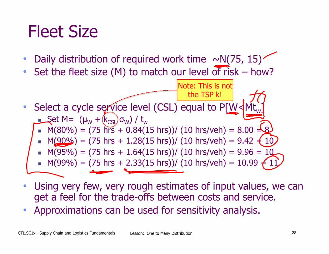
•  Daily distribution of required work time ~N(75, 15) •  Set the fleet size (M) to match our level of risk – how?

•  Select a cycle service level (CSL) equal to P[W<Mtw] n  Set M= (µW + kCSL σW) / tw n  M(80%) = (75 hrs + 0.84(15 hrs))/ (10 hrs/veh) = 8.00 = 8 n  M(90%) = (75 hrs + 1.28(15 hrs))/ (10 hrs/veh) = 9.42 = 10 n  M(95%) = (75 hrs + 1.64(15 hrs))/ (10 hrs/veh) = 9.96 = 10 n  M(99%) = (75 hrs + 2.33(15 hrs))/ (10 hrs/veh) = 10.99 = 11

•  Using very few, very rough estimates of input values, we can get a feel for the trade-offs between costs and service.

•  Approximations can be used for sensitivity analysis.

Note: This is not the TSP k!

Fleet Size

28


Key Take Aways


Key Take Aways •  Many forms of product flow: One-to-One, One-to-Many,

Many-to-One, and Many-to-Many •  Approximations are good “first steps”

n  Require minimal data n  Allow for fast sensitivity analysis n  Enables quick scoping of the solution space

•  Optimal methods usually require tremendous amounts of detailed information

•  Planning problems usually have lots of uncertainty – the actual conditions are unknown

•  Before deciding to spend the time and energy to find an optimal solution, it is helpful to see if it is worth it.

30

MIT Center for Transportation & Logistics

CTL.SC1x -Supply Chain & Logistics Fundamentals

Questions, Comments, Suggestions? Use the Discussion!

[email protected]

“Dexter – continuously approximating” Yankee Golden Retriever Rescued Dog

(www.ygrr.org)

one to many distribution - edxmitx+ctl.sc1x_1+2... · one to many distribution . ... factors for...

Documents