ONLINE APPENDIX

"Explaining Social Policy Preferences: Evidence from the Great Recession Yotam Margalit, APSR (2013)

Survey items used in the analysis

[Welfare policy preferences]: Do you support an increase in the funding of government programs for

helping the poor and the unemployed with education, training, employment, and social services, even if

this would raise your taxes?

(1) Strongly oppose; (2) Somewhat oppose; (3) Neither support nor oppose; (4) Somewhat support; (5)

Strongly support

How important should it be for the government to do each of the following things:

[Global Warming] Protect the environment from global warming.

[National Security] Protect its borders from security threats.

[American Values] Protect American values from foreign cultural influences.

(1) Very important; (2) Somewhat important; (3) Neither important nor unimportant (4) Somewhat

unimportant (5) Completely unimportant

[Employment Status]: Are you currently employed?

Full-time employee; Part time employee; Self-employed; Unemployed; Retired; Student; Homemaker

[Household Income]: variable was coded based on the following question: Can you give us an estimate of

your salary in 2008 before taxes?

Below $30,000; $30,000 - $40,000; $40,000 - 50,000; $50,000 - $60,000; $60,000 - $75,000; $75,000 -

$90,000; $90,000 - $110,000; $110,000 - $130,000; $130,000 - $150,000; Over $150,000

Note that the question was asked separately for the respondent’s income and for that of their spouse. The

top category was capped at $160,000. The results were converted into U.S. dollar figures, taking the mid-

point of each band, and summed up for both self and spouse.

Job Security: Looking forward to the next three years, how confident do you feel about being able to keep

your current job?

1. Very confident 2. Confident. 3. Slightly confident. 4. Not at all confident

Education: What is the highest level of education you have completed?

Did not graduate from high school

High school graduate

Some college, but no degree (yet)

2-year college degree

4-year college degree

Postgraduate degree (MA, MBA, MD, JD, PhD, etc.)

Party Identification: Generally speaking, do you think of yourself as a ...?

Democrat; Republican; Independent; Other; Not sure

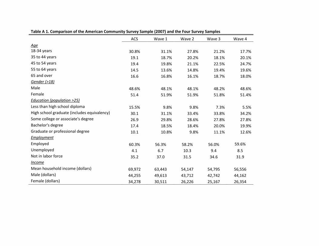
Table A 1. Comparison of the American Community Survey Sample (2007) and the Four Survey Samples

ACS Wave 1 Wave 2 Wave 3 Wave 4

Age

18-34 years 30.8% 31.1% 27.8% 21.2% 17.7% 35 to 44 years 19.1 18.7% 20.2% 18.1% 20.1% 45 to 54 years 19.4 19.8% 21.1% 22.5% 24.7% 55 to 64 years 14.5 13.6% 14.8% 19.4% 19.6% 65 and over 16.6 16.8% 16.1% 18.7% 18.0% Gender (>18)

Male 48.6% 48.1% 48.1% 48.2% 48.6% Female 51.4 51.9% 51.9% 51.8% 51.4% Education (population >25)

Less than high school diploma 15.5% 9.8% 9.8% 7.3% 5.5% High school graduate (includes equivalency) 30.1 31.1% 33.4% 33.8% 34.2% Some college or associate's degree 26.9 29.8% 28.6% 27.8% 27.8% Bachelor's degree 17.4 18.5% 18.4% 20.0% 19.9% Graduate or professional degree 10.1 10.8% 9.8% 11.1% 12.6% Employment

Employed 60.3% 56.3% 58.2% 56.0% 59.6%

Unemployed 4.1 6.7 10.3 9.4 8.5 Not in labor force 35.2 37.0 31.5 34.6 31.9 Income

Mean household income (dollars) 69,972 63,443 54,147 54,795 56,556 Male (dollars) 44,255 49,613 43,712 42,742 44,162 Female (dollars) 34,278 30,511 26,226 25,167 26,354

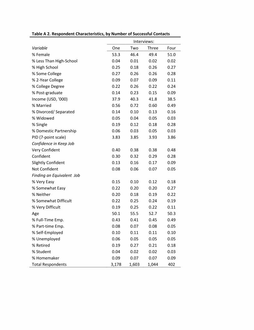
Table A 2. Respondent Characteristics, by Number of Successful Contacts

Interviews:

Variable One Two Three Four

% Female 53.3 46.4 49.4 51.0

% Less Than High-School 0.04 0.01 0.02 0.02

% High School 0.25 0.18 0.26 0.27

% Some College 0.27 0.26 0.26 0.28

% 2-Year College 0.09 0.07 0.09 0.11

% College Degree 0.22 0.26 0.22 0.24

% Post-graduate 0.14 0.23 0.15 0.09

Income (USD, '000) 37.9 40.3 41.8 38.5

% Married 0.56 0.72 0.60 0.49

% Divorced/ Separated 0.14 0.10 0.13 0.16

% Widowed 0.05 0.04 0.05 0.03

% Single 0.19 0.12 0.18 0.28

% Domestic Partnership 0.06 0.03 0.05 0.03

PID (7-point scale) 3.83 3.85 3.93 3.86

Confidence in Keep Job Very Confident 0.40 0.38 0.38 0.48

Confident 0.30 0.32 0.29 0.28

Slightly Confident 0.13 0.16 0.17 0.09

Not Confident 0.08 0.06 0.07 0.05

Finding an Equivalent Job % Very Easy 0.15 0.10 0.12 0.18

% Somewhat Easy 0.22 0.20 0.20 0.27

% Neither 0.20 0.18 0.19 0.22

% Somewhat Difficult 0.22 0.25 0.24 0.19

% Very Difficult 0.19 0.25 0.22 0.11

Age 50.1 55.5 52.7 50.3

% Full-Time Emp. 0.43 0.41 0.45 0.49

% Part-time Emp. 0.08 0.07 0.08 0.05

% Self-Employed 0.10 0.11 0.11 0.10

% Unemployed 0.06 0.05 0.05 0.05

% Retired 0.19 0.27 0.21 0.18

% Student 0.04 0.02 0.02 0.03

% Homemaker 0.09 0.07 0.07 0.09

Total Respondents 3,178 1,603 1,044 402

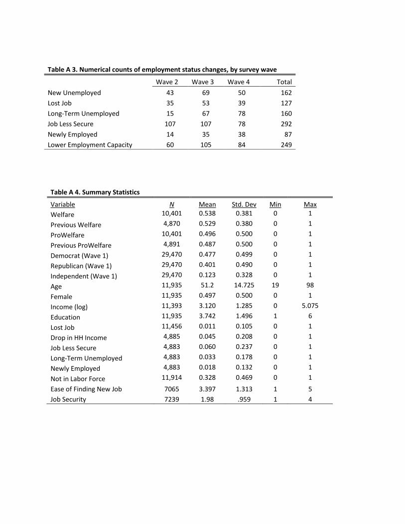
Table A 3. Numerical counts of employment status changes, by survey wave

Wave 2 Wave 3 Wave 4 Total

New Unemployed 43 69 50 162

Lost Job 35 53 39 127

Long-Term Unemployed 15 67 78 160

Job Less Secure 107 107 78 292

Newly Employed 14 35 38 87

Lower Employment Capacity 60 105 84 249

Table A 4. Summary Statistics

Variable N Mean Std. Dev Min Max

Welfare 10,401 0.538 0.381 0 1

Previous Welfare 4,870 0.529 0.380 0 1

ProWelfare 10,401 0.496 0.500 0 1

Previous ProWelfare 4,891 0.487 0.500 0 1

Democrat (Wave 1) 29,470 0.477 0.499 0 1

Republican (Wave 1) 29,470 0.401 0.490 0 1

Independent (Wave 1) 29,470 0.123 0.328 0 1

Age 11,935 51.2 14.725 19 98

Female 11,935 0.497 0.500 0 1

Income (log) 11,393 3.120 1.285 0 5.075

Education 11,935 3.742 1.496 1 6

Lost Job 11,456 0.011 0.105 0 1

Drop in HH Income 4,885 0.045 0.208 0 1

Job Less Secure 4,883 0.060 0.237 0 1

Long-Term Unemployed 4,883 0.033 0.178 0 1

Newly Employed 4,883 0.018 0.132 0 1

Not in Labor Force 11,914 0.328 0.469 0 1

Ease of Finding New Job 7065 3.397 1.313 1 5

Job Security 7239 1.98 .959 1 4

5

Table A 5. Economic shocks and difference in support for welfare spending, by party ID

Economic Shock

Party ID (in t=1) Loss

of Job Income Decline

Job Less Secure

Democrats 4% -5% 4%

Republicans 19% 7% 8%

Independents 23% 10% 6%

Affected Individuals (127) (222) (292)

Note: Entries denote the unconditional differencing of change in support for expanding welfare spending, comparing the policy preferences of those personally affected and those unaffected by the economic shock. To make the comparison meaningful, in the first two columns the sample is restricted only to individuals that were employed in the previous period. *Figures in parentheses denote the number of individuals affected by each shock.

6

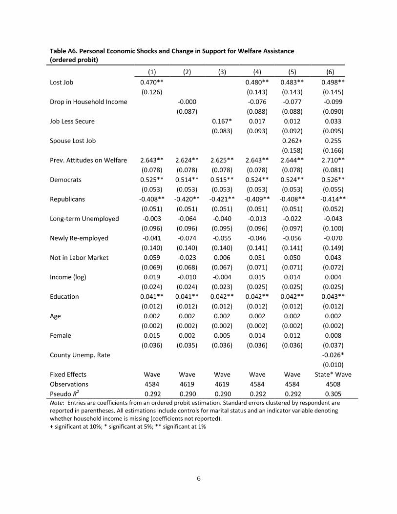
Table A6. Personal Economic Shocks and Change in Support for Welfare Assistance (ordered probit)

(1) (2) (3) (4) (5) (6)

Lost Job 0.470**

0.480** 0.483** 0.498**

(0.126)

(0.143) (0.143) (0.145)

Drop in Household Income

-0.000

-0.076 -0.077 -0.099

(0.087)

(0.088) (0.088) (0.090)

Job Less Secure

0.167* 0.017 0.012 0.033

(0.083) (0.093) (0.092) (0.095)

Spouse Lost Job

0.262+ 0.255

(0.158) (0.166)

Prev. Attitudes on Welfare 2.643** 2.624** 2.625** 2.643** 2.644** 2.710**

(0.078) (0.078) (0.078) (0.078) (0.078) (0.081)

Democrats 0.525** 0.514** 0.515** 0.524** 0.524** 0.526**

(0.053) (0.053) (0.053) (0.053) (0.053) (0.055)

Republicans -0.408** -0.420** -0.421** -0.409** -0.408** -0.414**

(0.051) (0.051) (0.051) (0.051) (0.051) (0.052)

Long-term Unemployed -0.003 -0.064 -0.040 -0.013 -0.022 -0.043

(0.096) (0.096) (0.095) (0.096) (0.097) (0.100)

Newly Re-employed -0.041 -0.074 -0.055 -0.046 -0.056 -0.070

(0.140) (0.140) (0.140) (0.141) (0.141) (0.149)

Not in Labor Market 0.059 -0.023 0.006 0.051 0.050 0.043

(0.069) (0.068) (0.067) (0.071) (0.071) (0.072)

Income (log) 0.019 -0.010 -0.004 0.015 0.014 0.004

(0.024) (0.024) (0.023) (0.025) (0.025) (0.025)

Education 0.041** 0.041** 0.042** 0.042** 0.042** 0.043**

(0.012) (0.012) (0.012) (0.012) (0.012) (0.012)

Age 0.002 0.002 0.002 0.002 0.002 0.002

(0.002) (0.002) (0.002) (0.002) (0.002) (0.002)

Female 0.015 0.002 0.005 0.014 0.012 0.008

(0.036) (0.035) (0.036) (0.036) (0.036) (0.037)

County Unemp. Rate -0.026*

(0.010)

Fixed Effects Wave Wave Wave Wave Wave State* Wave

Observations 4584 4619 4619 4584 4584 4508

Pseudo R2 0.292 0.290 0.290 0.292 0.292 0.305 Note: Entries are coefficients from an ordered probit estimation. Standard errors clustered by respondent are reported in parentheses. All estimations include controls for marital status and an indicator variable denoting whether household income is missing (coefficients not reported). + significant at 10%; * significant at 5%; ** significant at 1%

7

Table A7. Comparison of Demographic Characteristics: Newly Re-Employed Still Unemployed

Demographic Newly Re-employed (prev. unemployed)

Still Unemployed

Age 18_34 24.1% 8.1%

Age 35-44 19.5% 19.4%

Age 45-54 32.3% 37.5%

Age 55-64 20.6% 32.5%

Age 65+ 2.3% 2.5%

Female 51.7% 52.5%

White 71.3% 75.6%

Black 10.3% 13.1%

Hispanic 11.5% 6.9%

Less than High-School 2.3% 5.0%

High School 25.3% 29.4%

Some College 34.5% 29.4%

College 26.4% 26.9%

Graduate 11.5% 9.4% Married/Domestic Partnership 43.7% 40.6%

Separated/Divorced 14.9% 18.1%

Single 40.2% 38.1%

8

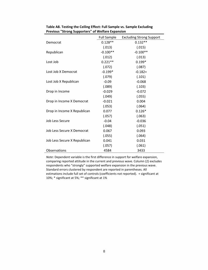
Table A8. Testing the Ceiling Effect: Full Sample vs. Sample Excluding Previous "Strong Supporters" of Welfare Expansion

Full Sample Excluding Strong Support

Democrat 0.128** 0.132**

(.013) (.015)

Republican -0.100** -0.100**

(.012) (.013)

Lost Job 0.221** 0.199*

(.072) (.087)

Lost Job X Democrat -0.199* -0.182+

(.079) (.101)

Lost Job X Republican -0.09 -0.068

(.089) (.103)

Drop in Income -0.029 -0.072

(.049) (.055)

Drop in Income X Democrat -0.021 0.004

(.053) (.064)

Drop in Income X Republican 0.077 0.126*

(.057) (.063)

Job Less Secure -0.04 -0.036

(.048) (.051)

Job Less Secure X Democrat 0.067 0.093

(.055) (.064)

Job Less Secure X Republican 0.041 0.031

(.057) (.061)

Observations 4584 3433

Note: Dependent variable is the first difference in support for welfare expansion, comparing reported attitude in the current and previous wave. Column (2) excludes respondents who “strongly” supported welfare expansion in the previous wave. Standard errors clustered by respondent are reported in parentheses. All estimations include full set of controls (coefficients not reported). + significant at 10%; * significant at 5%; ** significant at 1%

9

Note on the use of weights: All the analyses reported in the manuscript, which aim to portray the

preference of the U.S. public at a given time period, are calculated using sample weights (i.e.

Figures 2 and 3). The weights were constructed to make each wave representative of the U.S.

population in terms of key demographics. Note that these analyses also include respondents that

are not part of the panel, but which were interviewed by YouGov in order to make the sample

wave more similar in terms of demographic characteristics to the overall public. In contrast, all

analyses that examine change in policy preference at the individual level (i.e. the remaining

tables and graphs) are calculated without weights, since one seeks to estimate the effect of a

given change in circumstances at the individual level, without claims about of the impact on the

U.S. electorate at large. I believe that by presenting the unweighted comparisons, the analysis

provides readers a clearer sense of how to interpret the estimated effects, without having to

worry that the effects are an artifact of the weighting. Nonetheless, I should add that including

the sample weights in the regressions makes the results stronger than those reported in the article,

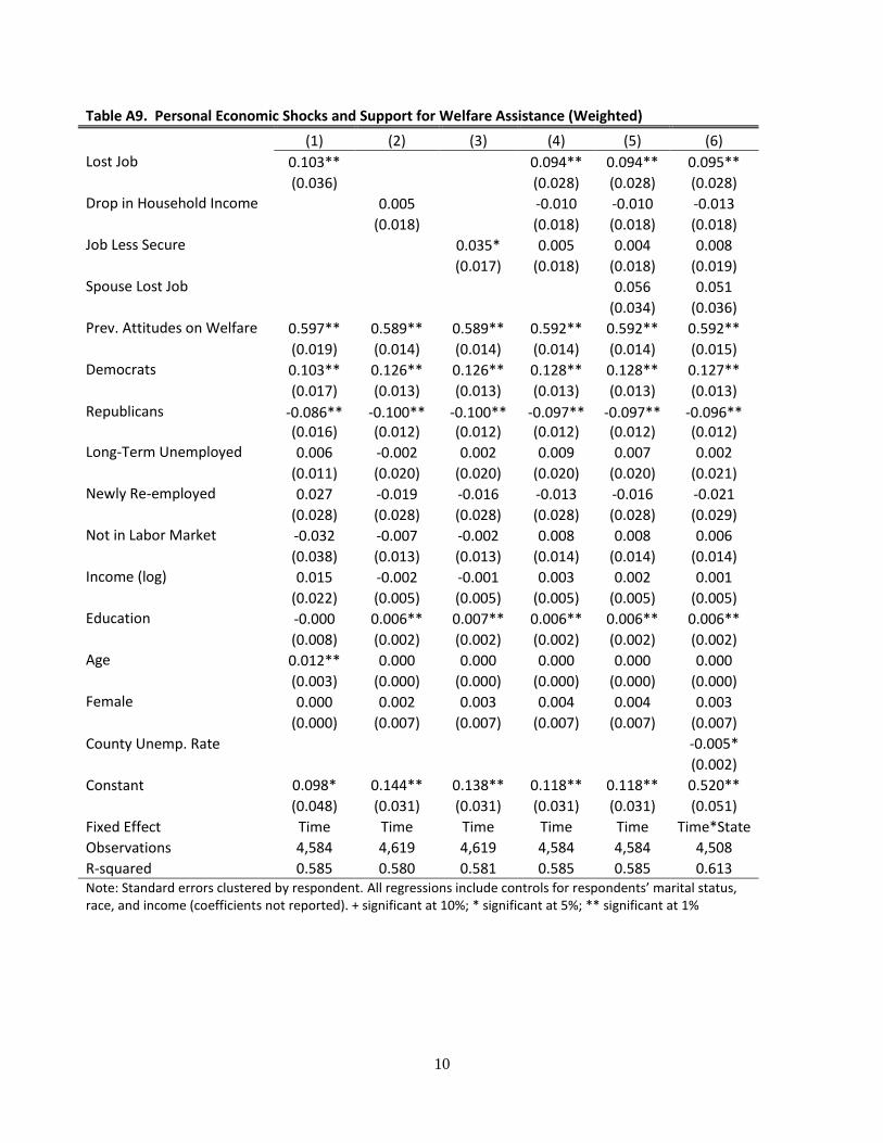
not weaker. To demonstrate the difference from including the weights, in Table A9 I replicate

the analysis presented in Table 3 of the manuscript, this time using sampling weights. As one can

see, all the estimated effects of interest remain robust as before while the point estimates are

slightly larger than in the unweighted specification.

10

Table A9. Personal Economic Shocks and Support for Welfare Assistance (Weighted)

(1) (2) (3) (4) (5) (6)

Lost Job 0.103**

0.094** 0.094** 0.095**

(0.036)

(0.028) (0.028) (0.028)

Drop in Household Income

0.005

-0.010 -0.010 -0.013

(0.018)

(0.018) (0.018) (0.018)

Job Less Secure

0.035* 0.005 0.004 0.008

(0.017) (0.018) (0.018) (0.019)

Spouse Lost Job

0.056 0.051

(0.034) (0.036)

Prev. Attitudes on Welfare 0.597** 0.589** 0.589** 0.592** 0.592** 0.592**

(0.019) (0.014) (0.014) (0.014) (0.014) (0.015)

Democrats 0.103** 0.126** 0.126** 0.128** 0.128** 0.127**

(0.017) (0.013) (0.013) (0.013) (0.013) (0.013)

Republicans -0.086** -0.100** -0.100** -0.097** -0.097** -0.096**

(0.016) (0.012) (0.012) (0.012) (0.012) (0.012)

Long-Term Unemployed 0.006 -0.002 0.002 0.009 0.007 0.002

(0.011) (0.020) (0.020) (0.020) (0.020) (0.021)

Newly Re-employed 0.027 -0.019 -0.016 -0.013 -0.016 -0.021

(0.028) (0.028) (0.028) (0.028) (0.028) (0.029)

Not in Labor Market -0.032 -0.007 -0.002 0.008 0.008 0.006

(0.038) (0.013) (0.013) (0.014) (0.014) (0.014)

Income (log) 0.015 -0.002 -0.001 0.003 0.002 0.001

(0.022) (0.005) (0.005) (0.005) (0.005) (0.005)

Education -0.000 0.006** 0.007** 0.006** 0.006** 0.006**

(0.008) (0.002) (0.002) (0.002) (0.002) (0.002)

Age 0.012** 0.000 0.000 0.000 0.000 0.000

(0.003) (0.000) (0.000) (0.000) (0.000) (0.000)

Female 0.000 0.002 0.003 0.004 0.004 0.003

(0.000) (0.007) (0.007) (0.007) (0.007) (0.007)

County Unemp. Rate

-0.005*

(0.002)

Constant 0.098* 0.144** 0.138** 0.118** 0.118** 0.520**

(0.048) (0.031) (0.031) (0.031) (0.031) (0.051)

Fixed Effect Time Time Time Time Time Time*State

Observations 4,584 4,619 4,619 4,584 4,584 4,508

R-squared 0.585 0.580 0.581 0.585 0.585 0.613 Note: Standard errors clustered by respondent. All regressions include controls for respondents’ marital status, race, and income (coefficients not reported). + significant at 10%; * significant at 5%; ** significant at 1%

11

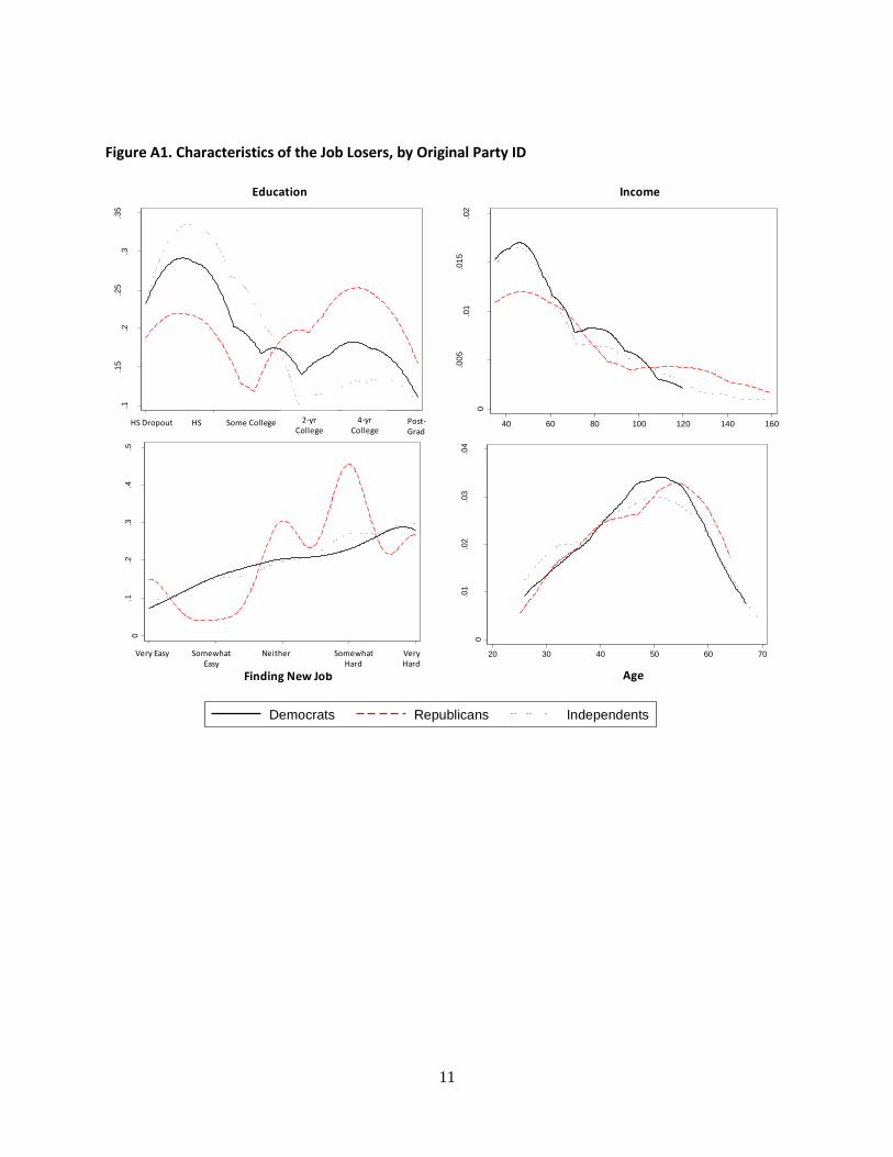
Figure A1. Characteristics of the Job Losers, by Original Party ID

0.1

.2.3

.4.5

Den

sity

1 2 3 4 5

0

.01

.02

.03

.04

Den

sity

20 30 40 50 60 70

0

.00

5.0

1.0

15

.02

Den

sity

40 60 80 100 120 140 160

Education Income

Finding New Job Age

.1.1

5.2

.25

.3.3

5

Den

sity

2 3 4 5 6HS Dropout HS Post-Grad

4-yr College

2-yr College

Some College

Very Easy Somewhat Easy

Very Hard

Somewhat Hard

Neither

0.1

.2.3

.4.5

Den

sity

1 2 3 4 5

Democrats Republicans Independents

12

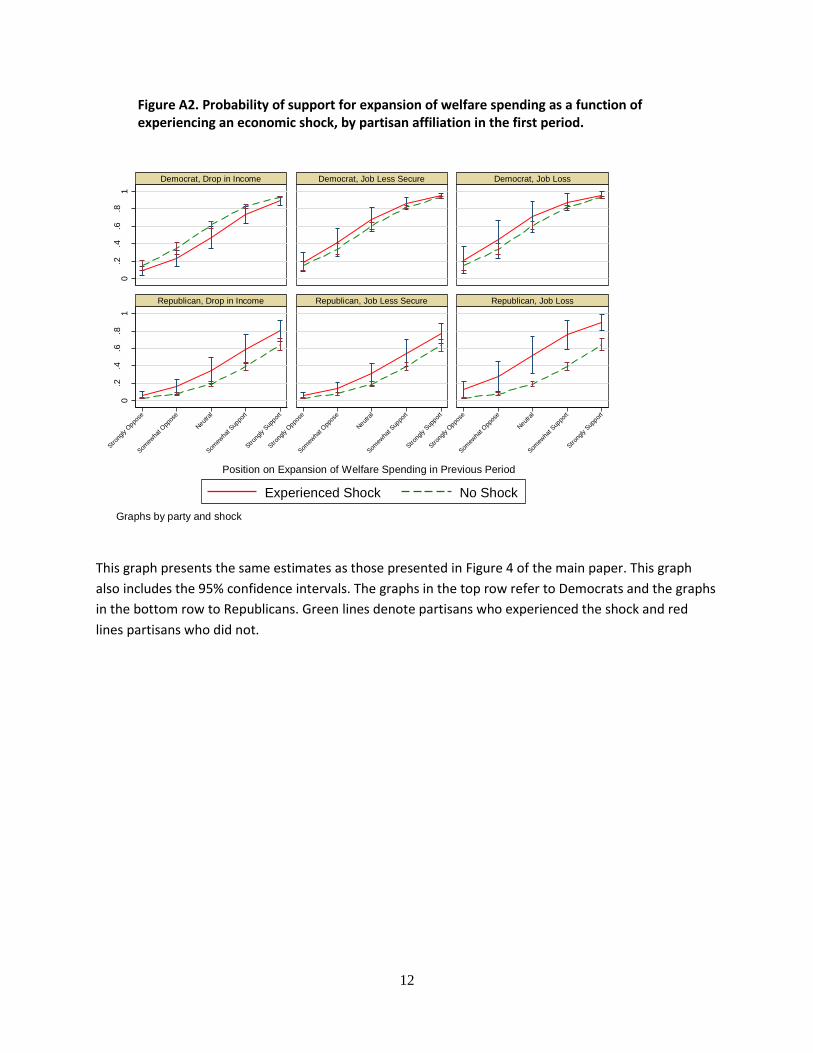
Figure A2. Probability of support for expansion of welfare spending as a function of experiencing an economic shock, by partisan affiliation in the first period.

This graph presents the same estimates as those presented in Figure 4 of the main paper. This graph

also includes the 95% confidence intervals. The graphs in the top row refer to Democrats and the graphs

in the bottom row to Republicans. Green lines denote partisans who experienced the shock and red

lines partisans who did not.

0.2

.4.6

.81

0.2

.4.6

.81

Strong

ly O

ppose

Somew

hat O

ppos

e

Neut

ral

Somew

hat S

uppo

rt

Strong

ly S

uppor

t

Strong

ly O

ppose

Somew

hat O

ppos

e

Neut

ral

Somew

hat S

uppo

rt

Strong

ly S

uppor

t

Strong

ly O

ppose

Somew

hat O

ppos

e

Neut

ral

Somew

hat S

uppo

rt

Strong

ly S

uppor

t

Democrat, Drop in Income Democrat, Job Less Secure Democrat, Job Loss

Republican, Drop in Income Republican, Job Less Secure Republican, Job Loss

Experienced Shock No Shock

Position on Expansion of Welfare Spending in Previous Period

Graphs by party and shock

13

APPENDIX B

Attitude Change on Welfare Policy-Related Questions: Comparison of YouGov vs. Pew Research Data

A concern one must have with results from any given survey study is the question of external

validity. To what extent is the sample used in the study representative of the population whose

attitudes it seeks to measure? To help address this question, I compare the responses to the Main

Question explored in this article with a question asked as part of the Pew Research’s study

“Trends in Political Values and Core Attitudes”. The question, read over the phone to three

different nationally-representative samples in three waves – December 2007; April 2009, and

April 2012 , read as follows:

The government should help more needy people even if it means going deeper in debt? Do you

completely agree, mostly agree, mostly disagree, or completely disagree?

The Pew Question and the Main Question are not quite the same. Most obviously, the Pew

Question does not mention assistance to the unemployed, the trade-off it mentions is higher debt

rather than higher taxes, and the time-period it covers is not identical to the panel study I use.

Moreover, the Pew Question did not offer a neutral or mid-point response option. Nonetheless, it

asks about support for assistance to the needy and also mentions a potential tradeoff, in this case

an increase in the national debt which would imply either lower spending in the future, higher

taxes, or perhaps both. Thus, it captures some of the same tradeoff between a more expansive

social safety net and higher future burden.

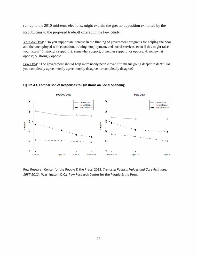
The results obtained in each of the two studies are presented in the figure below. The results of

the Pew study are reassuring in that they appear to confirm the main temporal trends observed in

the YouGov study analyzed in the article. These include: (i) a large and consistent partisan divide

in support for welfare spending over the time period under study; (ii) a general trend of

decreasing support for expanded welfare spending among all three partisan groups; (iii) a largest

drop in support among Independents; (iv) a drop in support among Democrats immediately

following the eruption of the crisis and then a tapering off of the effect. The one difference we

do observe between the two studies is the larger drop in support among Republicans that is

observed in the Pew Study. It is difficult to tell why this is the case, though perhaps the explicit

mention of the debt increase, an issue which was the rallying cry of the Republicans during the

14

run-up to the 2010 mid-term elections, might explain the greater opposition exhibited by the

Republicans to the proposed tradeoff offered in the Pew Study.

YouGov Data: “Do you support an increase in the funding of government programs for helping the poor

and the unemployed with education, training, employment, and social services, even if this might raise

your taxes?” 1. strongly support; 2. somewhat support; 3. neither support nor oppose; 4. somewhat

oppose; 5. strongly oppose.

Pew Data: “The government should help more needy people even if it means going deeper in debt” Do

you completely agree, mostly agree, mostly disagree, or completely disagree?

Figure A3. Comparison of Responses to Questions on Social Spending

Pew Research Center for the People & the Press. 2012. Trends in Political Values and Core Attitudes:

1987-2012. Washington, D.C.: Pew Research Center for the People & the Press.

15

APPENDIX C

The experiment was administered as follows: respondents were randomly assigned to receive one

of the treatments below. Each treatment was assigned to approximately 170 respondents. The

question was added in the beginning of an omnibus survey administered by YouGov/Polimetrix,

CA, in June 2012. Following the survey question, respondents were prompted with a set of five

response options: 1. strongly support; 2. somewhat support; 3. neither support nor oppose; 4.

somewhat oppose; 5. strongly oppose. The versions of the question assigned to each treatment

were as follows:

Version I: “Main Question” (The original item used as the dependent variable in the article)

Do you support an increase in the funding of government programs for helping the poor and the

unemployed with education, training, employment, and social services, even if this might raise

your taxes?

Version II: No Tradeoff

Do you support an increase in the funding of government programs for helping the poor and the

unemployed with education, training, employment, and social services?

Version III: Unemployed, Active Labor-Market Programs

Do you support an increase in the funding of government programs for helping the unemployed

with education, training, and employment, even if this might raise your taxes?

Version IV: Needy, Social Services

Do you support an increase in the funding of government programs for helping the poor with

social services, even if this might raise your taxes?

Table A10. Support for Expanded Welfare Provision, by Experimental Treatment

All N Democrats N Republicans N

Version I: Original 45.0% (169) 74.3% (74) 14.3% (63)

Version II: Original_No Tradeoff 51.8% (168) 75.6% (78) 22.6% (62)

Version III: Unemployed_ALP 46.4% (168) 71.6% (74) 17.9% (67)

Version IV: Needy_Welfare 47.6% (168) 74.0% (77) 15.4% (65)