online appendix for the paper fithe impact of
TRANSCRIPT

Online Appendix for the paper �The Impact of IntergovernmentalTransfers on Education Outcomes and Poverty Reduction�
Stephan Litschig and Kevin Morrison
February 27, 2013
List of Figures
1 Figure 1: McCrary density plots and discontinuity tests for cutoffs 1 through 6 . . . 11
2 Figure 2: Impacts on total spending and main spending categories . . . . . . . . . 12
3 Figure 3: Impacts on direct public service measures . . . . . . . . . . . . . . . . . 13
List of Tables
1 Table 1: Discontinuity tests for pretreatment covariates (quadratic speci�cations) . 14
2 Table 2: Impacts on spending categories . . . . . . . . . . . . . . . . . . . . . . . 15
3 Table 3: Impact on teacher-student ratio . . . . . . . . . . . . . . . . . . . . . . . 16
4 Table 5.1: Robustness checks for impact on schooling, 19- to 28-year-olds in 1991 17
5 Table 6.1: Robustness checks for impact on schooling, 9- to 18-year-olds in 1991 . 18
6 Table 5.2: Impact on change in schooling, 19- to 28-year-olds in 1991 . . . . . . . 19
7 Table 5.3: Impact on change in schooling, above 24 year-olds in 1980 . . . . . . . 20
8 Table 5.4: Schooling gains for native nonmigrants, 19- to 28-year-olds in 1991 . . . 21
9 Table 7.1: Robustness checks for impact on literacy, 19- to 28-year-olds in 1991 . . 22
10 Table 7.2: Impact on literacy, 9- to 18-year-olds in 1991 . . . . . . . . . . . . . . . 23
11 Table 7.3: Robustness checks for impact on literacy, 9- to 18-year-olds in 1991 . . 24
12 Table 7.4: Impact on change in literacy, 19- to 28-year-olds in 1991 . . . . . . . . 25
13 Table 7.5: Literacy gains for native nonmigrants, 19- to 28-year-olds in 1991 . . . 26
14 Table 8.1: Robustness checks for impact on the poverty rate in 1991 . . . . . . . . 27
1
15 Table 9.1: Impact on the probability of reelection (nonlinear speci�cations) . . . . 28
16 Table 10: Joint signi�cance test of education, income and public service outcomes . 29
17 Table 11: Total spending and teacher-student ratio, north vs. south . . . . . . . . . 30
18 Table 12: Schooling, literacy and poverty, north vs. south . . . . . . . . . . . . . . 31
19 Table 13: Total spending and teacher-student ration, urban vs. rural municipalities . 32
20 Table 14: Schooling, literacy, poverty, urban vs. rural municipalities . . . . . . . . 33
2

1 Impacts on spending shares
Figure 2 documents the impacts of additional FPM funding on total spending per capita as well as
on the main local expenditure categories: education, housing and urban infrastructure, and trans-
portation. There is clear evidence of a jump of about 20% at the cutoff in all of these variables,
although the jumps in expenditure categories are somewhat sensitive to the width of the neigh-
borhood examined. The regression lines also slope downward almost without exception, which is
further evidence favoring the validity of the design. The spending category graphs are considerably
noisier than the total spending graph because the sample size is smaller (due to missing values) and
because the expenditure categories are only available for the years 1982 and 1983, whereas total
spending is reported over the entire period 1982 to 1985. Nevertheless, the jumps in the expendi-
ture categories are also statistically signi�cant as shown in Table 2. This evidence thus suggests
that local spending on education, housing and urban infrastructure, and transportation all increased
by about 20% per capita, leaving local spending shares essentially unchanged.1
2 Impacts on direct public service measures
The public service indicators we consider are dictated by data availability. They are measured in
1991, the earliest posttreatment year for which comprehensive data on municipalities are available.
The indicators are supposed to capture improvements in the main spending areas of education as
well as housing and urban infrastructure. Unfortunately we do not have any indicators on local
transportation services or infrastructure.
In the area of education, we use the primary school teacher-student ratio in municipal elemen-
tary schools and the number of schools run by the municipal government. It is easy to see how
extra spending over the period 1982-1985 might affect the number of schools six years later in
1991. Effects on teacher-student ratios in 1991 might arise if the extra spending on education
was in fact smoothed over subsequent years or if additional teachers could not easily be dismissed
once the funding differential stopped. Public service measures in the area of housing and urban
infrastructure are the percentages of individuals in the municipality with access to water, sewer,1To be precise, the null hypothesis of a proportional, 20 percent per capita increase cannot be rejected in any of the
speci�cations.
3

electricity and living in substandard housing.
Table 3 shows effects on the primary school teacher-student ratio. Estimates are reasonably
close across samples and suggest that the teacher-student ratio increased by about .01, or one
teacher per hundred students. This compares to an average teacher-student ratio in the marginal
comparison group of about .05. The implied average class-size reduction at the primary school
level amounts to about 3 students per teacher. In contrast, results on municipal elementary schools
(not shown) display no clear patterns and are imprecisely estimated, suggesting that transfers �-
nanced mostly more labor input as opposed to school infrastructure.
Housing and urban infrastructure measures do not indicate much evidence of public service
improvements. Although the estimates go almost all in the right direction (positive for access to
electricity, water and sewer; negative for inadequate housing) they are very variable and only rarely
statistically signi�cant. Rather than showing separate tables with mostly insigni�cant results, we
present the school and infrastructure estimates below when we test the joint signi�cance of all
the outcome variables. Figure 3 shows the results for the teacher-student ratio, elementary schools,
and water and electricity access graphically (the graphs for sewer and inadequate housing look very
similar to the electricity graph). Direct evidence on public service improvements is thus mixed at
best: while there is evidence that student-teacher ratios in local primary school systems fell, there
is little evidence that housing and urban development spending affected housing conditions.
3 Further robustness checks
This section provides further robustness checks regarding functional form of both the running
variable (population) and of pretreatment covariates, as well estimates using the change in average
schooling and literacy outcomes over time, rather than the 1991 levels. The corresponding dif-
ference estimates are also presented for cohorts that had largely completed their education when
the extra funding started in 1982 and for whom one would expect smaller or no impacts. A �nal
robustness check on education outcomes uses only the subsample of individuals who were born in
the municipality and never moved away. All the previously discussed results turn out to be robust
to these additional tests. To conclude this section, we test and reject the joint null hypotheses of
no discontinuities in any outcome variable, suggesting that at least some of the impacts above are
4

real. This section starts out with robustness checks for schooling (3.1), followed by literacy (3.2),
and poverty (3.3), and concludes with the joint test (3.4).
3.1 Schooling
Table 5.1 presents pooled estimates across cutoffs c1 and c2, as well as c1; c2 and c3 for the
older cohorts of 19- to 28-year-olds in 1991 and for the three previously used bandwidths (p D
2%; 3% and 4%). For each bandwidth, Table 5.1 has 3 columns, corresponding to the following
speci�cations: �rst, linear population polynomial with pretreatment covariates as in Table 5 of the
paper but now including average years of schooling of the 8- to 17-year-olds in 1980 (19- to 28-
year-olds in 1991) based on the 1980 census microdata as an additional control; second, quadratic
population polynomial without covariates; and third, linear population polynomial with a quadratic
speci�cation of the pretreatment covariates. The corresponding results for the younger cohort of
9- to 18-year-olds in 1991 are presented in Table 6.1.
All estimates in Table 5.1 are positive and most of them fall in the 0.2 to 0.3 range, the same
result encountered in Table 5 of the paper for the speci�cations with covariates. And as before,
these estimates become statistically signi�cant (at 5%) even within a relatively small neighborhood
of +/- 3% around the cutoffs. Table 5.1 also gives results of three hypothesis tests, one for each of
the three speci�cations discussed above. The �rst is a t-test of the hypothesis that the coef�cient
on the pretreatment outcome is equal to one, as imposed in the �rst-difference speci�cation further
discussed below. This null hypothesis is never rejected across bandwidths and cutoffs (the lowest p-
value 0.15). The second test investigates the joint hypotheses that the coef�cients on the quadratic
population terms on either side of the cutoff are zero, that is, whether linearity of the population
polynomial can be rejected. As expected, there is no statistical evidence against linearity close to
the cutoff (p D 2% and 3%), although for the p D 4% bandwidth linearity is clearly rejected. The
third is an F-test for the joint hypotheses that the coef�cients on the quadratics in covariates are all
zero. It turns out that the statistical evidence against including covariates linearly is weak across
bandwidths and cutoffs.
Estimates of the schooling gains for the 9- to 18-year-old cohort in 1991 based on the same
speci�cations as above are presented in Table 6.1. The only difference with the above speci�cations
5

is that pretreatment average schooling for this cohort (0- to 7-year-olds in 1980) is not included
since the census only collects schooling information for those aged 5 or above. As in Table 6, the
discontinuity estimates �uctuate around 0.15 years per capita, again statistically signi�cant even
in the narrow samples around the cutoffs. Again there is no statistical evidence against linearity of
the population polynomial close to the cutoff .p D 2% and 3%) and only weak statistical evidence
against including covariates linearly.
Table 5.2 presents estimates where the dependent variable is the change in average years of
schooling between 1991 and 1980 of the older cohorts (19- to 28-year-olds in 1991). This approach
imposes a coef�cient of one on initial schooling of this cohort, rather than allowing the coef�cient
to be estimated as in Table 5.1 above. For each bandwidth, Table 5.2 has 3 columns, corresponding
to the following speci�cations: �rst, linear population polynomial without covariates; second,
quadratic population polynomial without covariates; and third, linear population polynomial with
covariates. Again, all estimates in Table 5.2 are positive, most of them fall in the 0.2 to 0.3 range
and they become statistically signi�cant even within a relatively small neighborhood of +/- 3%
around the cutoffs.
In contrast, the corresponding estimates based on changes in average schooling for those 25
years and older in 1980�typically considered to have completed most of their schooling�are
close to zero in magnitude (sometimes negative) and very far from statistical signi�cance as shown
in Table 5.3. These estimates are for the exact same cohorts for which Table 3 in the paper shows a
positive schooling differential before the extra funding had started. While it is reassuring that these
older cohorts did not experience any schooling gains, strictly speaking this is not a falsi�cation test.
Although one would expect smaller effects on education outcomes for cohorts that were beyond
regular elementary schooling age, the effect need not be zero since older cohorts might have at-
tended adult literacy programs that were promoted by the military government and offered through
the local administration, such as the MOBRAL (Movimento Brasileiro de Alfabetização). In fact
the difference in average years of schooling of these cohorts in the comparison group is about 0.32,
on average (Table 5.3). This would be consistent with roughly one out of three individuals among
those 25 years and older getting an extra year of schooling over the eleven-year-period from 1980
to 1991.
6

As a �nal robustness check, we also estimate the impact on schooling for the 19- to 28-year-
olds in 1991 on a restricted sample of individuals who were born in a given municipality and never
moved away. The results are shown in Table 5.4 and are again quantitatively close to those from the
unrestricted sample. This provides suggestive evidence that the schooling gains stem at least partly
from existing residents, rather than being driven by inmigration of more highly educated individu-
als in response to public service improvements. The results are only suggestive, however, because
there could be selective attrition among nonmigrants across treatment and comparison communi-
ties. In particular, more educated individuals might be more likely to stay in the municipality in
response to public service improvements.
3.2 Literacy
Table 7.1 presents robustness checks for literacy outcomes of the 19- to 28-year-olds in 1991 using
the same speci�cations as in Tables 5.1 and 6.1 above. As in Table 7 in the paper, the estimates in
Table 7.1 suggest a literacy gain of about four percentage points throughout, signi�cant even in the
+/- 2% window around the cutoffs. The hypothesis that the coef�cient on the pretreatment outcome
is equal to one is soundly rejected across bandwidths and cutoffs (p-values of 0.00), although this
turns out not to matter at all for the estimate of interest. Again as expected, there is no statistical
evidence against linearity of the population polynomial close to the cutoff (p D 2% and 3%)
although for the p=4% bandwidth linearity is again rejected. There is also only weak statistical
evidence across bandwidths and cutoffs against including covariates linearly.
Estimates of the literacy gains for the 9- to 18-year-old cohort in 1991 are presented in Table
7.2. Table 7.3 presents robustness checks. Estimated impacts are mostly around two to three
percentage points, again statistically signi�cant even in the discontinuity samples. As in Table 7.1,
Table 7.3 shows no statistical evidence against linearity of the population polynomial close to the
cutoff and strong evidence against including covariates linearly across bandwidths and cutoffs.
Table 7.4 presents estimates where the dependent variable is the difference in literacy rates
between 1991 and 1980 of the older cohorts (19- to 28-year-olds in 1991). Compared to the
estimates of about four percentage points in Tables 7 and 7.1, those in Table 7.4 suggest a slightly
lower literacy gain of about three percentage points, again statistically signi�cant even within a
7
relatively small neighborhood of +/- 3% around the cutoffs.
Table 7.5 presents the �nal robustness check for the literacy gains of the 19- to 28-year-olds
in 1991 based on the subsample of individuals who were born in a given municipality and never
moved away. The results are again quantitatively close to those from the unrestricted sample.
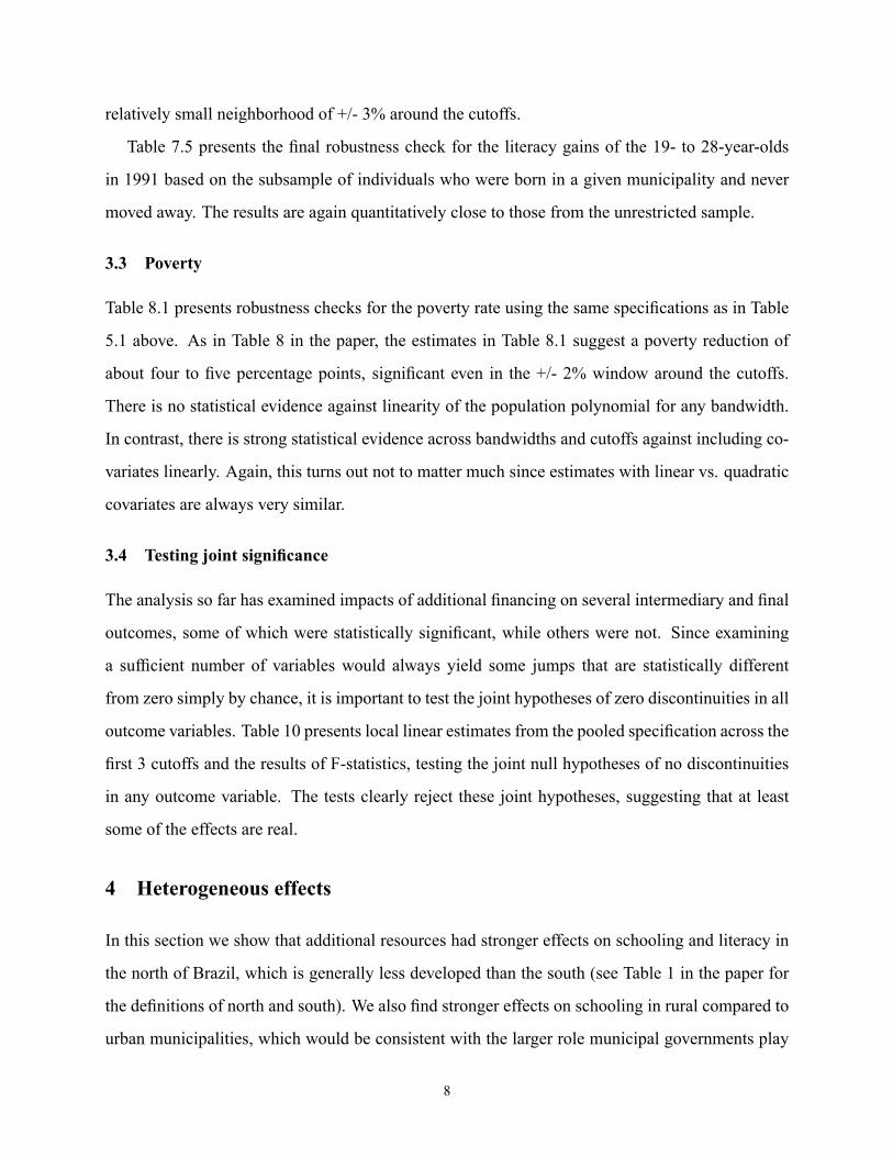
3.3 Poverty
Table 8.1 presents robustness checks for the poverty rate using the same speci�cations as in Table
5.1 above. As in Table 8 in the paper, the estimates in Table 8.1 suggest a poverty reduction of
about four to �ve percentage points, signi�cant even in the +/- 2% window around the cutoffs.
There is no statistical evidence against linearity of the population polynomial for any bandwidth.
In contrast, there is strong statistical evidence across bandwidths and cutoffs against including co-
variates linearly. Again, this turns out not to matter much since estimates with linear vs. quadratic
covariates are always very similar.
3.4 Testing joint signi�cance
The analysis so far has examined impacts of additional �nancing on several intermediary and �nal
outcomes, some of which were statistically signi�cant, while others were not. Since examining
a suf�cient number of variables would always yield some jumps that are statistically different
from zero simply by chance, it is important to test the joint hypotheses of zero discontinuities in all
outcome variables. Table 10 presents local linear estimates from the pooled speci�cation across the
�rst 3 cutoffs and the results of F-statistics, testing the joint null hypotheses of no discontinuities
in any outcome variable. The tests clearly reject these joint hypotheses, suggesting that at least
some of the effects are real.
4 Heterogeneous effects
In this section we show that additional resources had stronger effects on schooling and literacy in
the north of Brazil, which is generally less developed than the south (see Table 1 in the paper for
the de�nitions of north and south). We also �nd stronger effects on schooling in rural compared to
urban municipalities, which would be consistent with the larger role municipal governments play
8

in the provision of elementary education in rural areas. Poverty reduction was somewhat more
pronounced in the south of the country and evenly spread across rural and urban municipalities.
Table 11 shows impacts of additional FPM transfers on total public spending per capita and
on the primary school teacher-student ratio in northern and southern states of Brazil. Spending
increased by about 20% in both parts of the country and effects on primary school teacher-student
ratios tend to be positive and statistically signi�cant, especially in the south. Although all estimates
tend to be larger in the south they are not statistically different from each other. None of the other
public service indicators are statistically signi�cant in either region (results not shown).
Table 12 shows that the average schooling and literacy gains reported above are for the most
part accounted for by gains in the northern part of the country. The estimates with covariates put
the schooling gains in the north at about 0.3 years. Literacy gains are also larger in the north
than in the south. These regional differences in literacy and schooling gains are not statistically
signi�cant.2 The poverty reduction, in contrast, is larger in the south, and the differential impact is
statistically signi�cant.
Tables 13 and 14 examine whether the notion that extra funds have stronger effects in less
developed areas holds true not just between the northern and southern parts of Brazil but also
across rural and urban areas as distinguished by the median percentage of urban residents in 1980.
Table 13 shows that spending increased by about 20% in both urban and rural municipalities. The
effect on primary school teacher-student ratios tends to be positive and statistically signi�cant in
rural areas, with no real difference in urban areas although the differential effect is not statistically
signi�cant.3 Again, none of the other public service indicators are statistically signi�cant in either
region (results not shown).
The results in Table 14 suggest that almost the entire schooling gains come from rural munici-
palities (an additional 0.5 year of schooling per capita). Effects in urban communities are smaller,
statistically insigni�cant but not statistically different from the effects in rural communities.4 The
literacy gains are more evenly spread although they too are concentrated among rural municipali-2The coef�cients and standard errors on the interaction of the treatment indicator with the region indicator (1 for south)
in the pooled sample for schooling and literacy are, respectively: -0.172 (0.208) and - 0.033 (0.024).3The coef�cient and standard error on the interaction term of the treatment indicator with the urban indicator (1 for
urban) are -.007 and (.007).4The coef�cient and standard error on the interaction term are -.335 and (.221).
9

ties and somewhat smaller in urban municipalities although the difference is again not statistically
signi�cant.5 The poverty reduction is evenly spread across urban and rural communities. Overall,
the point estimates suggest that additional public spending had stronger effects on schooling and
literacy in less developed parts of Brazil, while poverty reduction was more pronounced in the
south of the country and evenly spread across rural and urban municipalities.6
An alternative explanation for these effects is that poor communities had stronger preferences
for education than richer communities and hence spent a higher proportion of extra funds on ed-
ucation. A direct test of this alternative view is to examine the share of education expenditure in
total spending subsequent to the increase in funding in poor vs. rich areas. Unfortunately, however,
existing expenditure data do not allow such a disaggregation between 1984 and 1989. When we
test for differential effects on education expenditure shares using data from 1982 and 1983, we
�nd no signi�cant effects (results not shown), suggesting that stronger preferences for education
in poor communities are not the driving force behind the higher schooling and literacy gains found
in less developed parts of Brazil.
5The coef�cient and standard error on the interaction term are -.005 and (.026).6We also break the sample into high vs. low education and low vs. high initial poverty counties and �nd quantitatively
similar results.
10
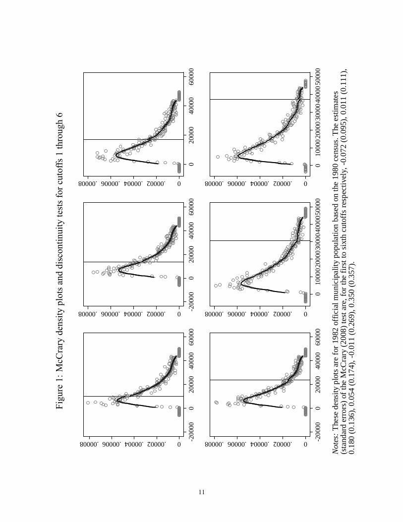
Figure1:McCrarydensityplotsanddiscontinuitytestsforcutoffs1through6
0.00002.00004.00006.00008 200
000
4000
060
000
2000
0
0.00002.00004.00006.00008 200
000
2000
040
000
6000
0
0.00002.00004.00006.00008
020
000
4000
060
000
0.00002.00004.00006.00008 200
000
2000
040
000
6000
0
0.00002.00004.00006.00008
010
0002
0000
3000
0400
0050
000
0.00002.00004.00006.00008
010
0002
0000
3000
0400
0050
000
Not
es: T
hese
den
sity
plo
ts a
re fo
r 198
2 of
ficia
l mun
icip
ality
pop
ulat
ion
base
d on
the
1980
cen
sus.
The
estim
ates
(sta
ndar
d er
rors
) of t
he M
cCra
ry (2
008)
test
are
, for
the
first
to s
ixth
cut
offs
resp
ectiv
ely,
0.0
72 (0
.095
), 0.
011
(0.1
11),
0.18
0 (0
.136
), 0.
054
(0.1
74),
0.0
11 (0
.269
), 0.
350
(0.3
57).
11
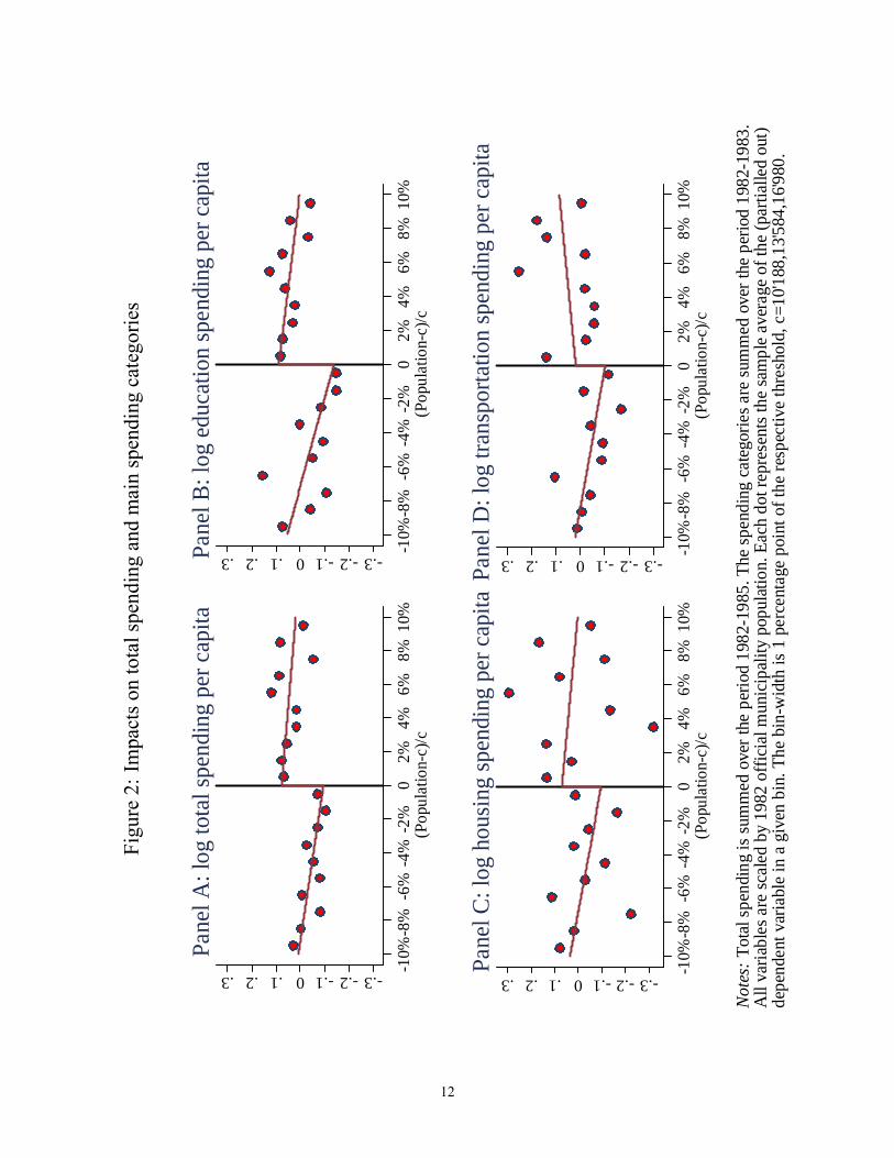
Figure2:Impactsontotalspendingandmainspendingcategories
.3.2.10.1.2.3 10%
8%
6%
4%
2%
02%
4%6%
8%10
%(P
opul
atio
nc)
/c
Pane
l A: l
og to
tal s
pend
ing
per c
apita
.3.2.10.1.2.3 10%
8%
6%
4%
2%
02%
4%6%
8%10
%(P
opul
atio
nc)
/c
Pane
l B: l
og e
duca
tion
spen
ding
per
cap
ita.3.2.10.1.2.3 1
0%8
%6
%4
%2
%0
2%4%
6%8%
10%
(Pop
ulat
ion
c)/c
Pane
l C: l
og h
ousin
g sp
endi
ng p
er c
apita
.3.2.10.1.2.3 10%
8%
6%
4%
2%
02%
4%6%
8%10
%(P
opul
atio
nc)
/c
Pane
l D: l
og tr
ansp
orta
tion
spen
ding
per
cap
ita
Note
s: T
otal
spen
ding
is su
mm
ed o
ver t
he p
erio
d 19
821
985.
The
spen
ding
cat
egor
ies a
re su
mm
ed o
ver t
he p
erio
d 19
821
983.
All
varia
bles
are
scal
ed b
y 19
82 o
ffici
al m
unic
ipal
ity p
opul
atio
n. E
ach
dot r
epre
sent
s the
sam
ple
aver
age
of th
e (p
artia
lled
out)
depe
nden
t var
iabl
e in
a g
iven
bin
. The
bin
wid
th is
1 p
erce
ntag
e po
int o
f the
resp
ectiv
e th
resh
old,
c=1
0'188
,13'5
84,1
6'980
.
12

Figure3:Impactsondirectpublicservicemeasures
.008.0040.004.008 10%
8%
6%
4%
2%
02%
4%6%
8%10
%(P
opul
atio
nc)
/c
Pane
l A: t
each
ers
tude
nt ra
tio
1050510 10%
8%
6%
4%
2%
02%
4%6%
8%10
%(P
opul
atio
nc)
/c
Pane
l B: n
umbe
r of e
lem
enta
ry sc
hool
s1050510 1
0%8
%6
%4
%2
%0
2%4%
6%8%
10%
(Pop
ulat
ion
c)/c
Pane
l C: a
cces
s to
wat
er (p
erce
nt)
1050510 10%
8%
6%
4%
2%
02%
4%6%
8%10
%(P
opul
atio
nc)
/c
Pane
l D: a
cces
s to
elec
trici
ty (p
erce
nt)
Not
es: E
ach
dot r
epre
sent
s th
e sa
mpl
e av
erag
e of
the
(par
tialle
d ou
t) de
pend
ent v
aria
ble
in a
giv
en b
in. T
he b
inw
idth
is 1
per
cent
age
poin
t of t
he re
spec
tive
thre
shol
d, c
=10'
188,
13'5
84,1
6'980
.
13
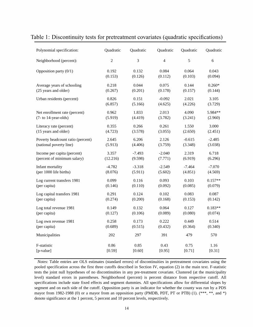
Table 1: Discontinuity tests for pretreatment covariates (quadratic speci�cations)
Polynomial specification: Quadratic Quadratic Quadratic Quadratic Quadratic
Neighborhood (percent): 2 3 4 5 6
Opposition party (0/1) 0.192 0.132 0.084 0.064 0.043(0.153) (0.126) (0.112) (0.103) (0.094)
Average years of schooling 0.218 0.044 0.075 0.144 0.260*(25 years and older) (0.267) (0.201) (0.178) (0.157) (0.144)
Urban residents (percent) 0.826 0.151 0.092 2.021 3.105(6.857) (5.166) (4.625) (4.226) (3.729)
Net enrollment rate (percent) 0.962 1.833 2.013 4.090 5.984**(7 to 14yearolds) (5.919) (4.419) (3.782) (3.241) (2.960)
Literacy rate (percent) 0.355 0.266 0.261 1.550 3.000(15 years and older) (4.723) (3.578) (3.055) (2.650) (2.451)
Poverty headcount ratio (percent) 2.645 6.206 2.126 0.615 2.485(national poverty line) (5.913) (4.406) (3.759) (3.348) (3.038)
Income per capita (percent) 3.357 7.493 2.040 2.319 6.718(percent of minimum salary) (12.216) (9.598) (7.771) (6.919) (6.296)
Infant mortality 4.782 3.318 2.549 7.464 7.070(per 1000 life births) (8.076) (5.911) (5.602) (4.851) (4.569)
Log current transfers 1981 0.099 0.116 0.093 0.103 0.157**(per capita) (0.146) (0.110) (0.092) (0.085) (0.079)
Log capital transfers 1981 0.291 0.124 0.102 0.083 0.087(per capita) (0.274) (0.200) (0.168) (0.153) (0.142)
Log total revenue 1981 0.149 0.132 0.064 0.127 0.183**(per capita) (0.127) (0.106) (0.089) (0.080) (0.074)
Log own revenue 1981 0.258 0.173 0.222 0.449 0.514(per capita) (0.689) (0.515) (0.432) (0.364) (0.340)
Municipalities 202 297 391 479 570
Fstatistic[pvalue]
0.86[0.59]
0.85[0.60]
0.43[0.95]
0.75[0.71]
1.16[0.31]
Notes: Table entries are OLS estimates (standard errors) of discontinuities in pretreatment covariates using thepooled specification across the first three cutoffs described in Section IV, equation (2) in the main text. Fstatistictests the joint null hypotheses of no discontinuities in any pretreatment covariate. Clustered (at the municipalitylevel) standard errors in parentheses. Neighborhood (percent) is percent distance from respective cutoff. Allspecifications include state fixed effects and segment dummies. All specifications allow for differential slopes bysegment and on each side of the cutoff. Opposition party is an indicator for whether the county was run by a PDSmayor from 19821988 (0) or a mayor from an opposition party (PMDB, PDT, PT or PTB) (1). (***, **, and *)denote significance at the 1 percent, 5 percent and 10 percent levels, respectively.
14
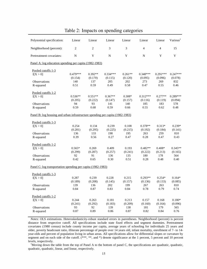
Table 2: Impacts on spending categories
Polynomial specification: Linear Linear Linear Linear Linear Linear Various1
Neighborhood (percent): 2 2 3 3 4 4 15
Pretreatment covariates: N Y N Y N Y Y
Panel A: log education spending per capita (19821983)
Pooled cutoffs 13I[X > 0] 0.479*** 0.392** 0.334*** 0.261** 0.348*** 0.291*** 0.247***
(0.154) (0.170) (0.115) (0.120) (0.095) (0.096) (0.078)Observations 140 137 205 202 273 269 832Rsquared 0.51 0.59 0.49 0.58 0.47 0.55 0.46
Pooled cutoffs 12I[X > 0] 0.536** 0.551** 0.367** 0.308* 0.312*** 0.277** 0.289***
(0.205) (0.222) (0.147) (0.157) (0.116) (0.119) (0.094)Observations 94 93 141 140 185 183 578Rsquared 0.59 0.68 0.59 0.66 0.55 0.62 0.48
Panel B: log housing and urban infrastructure spending per capita (19821983)
Pooled cutoffs 13I[X > 0] 0.254 0.134 0.239 0.108 0.378** 0.313* 0.239*
(0.281) (0.295) (0.225) (0.215) (0.192) (0.184) (0.141)Observations 136 133 198 195 263 259 810Rsquared 0.39 0.56 0.27 0.47 0.28 0.47 0.43
Pooled cutoffs 12 I[X > 0] 0.565* 0.269 0.409 0.193 0.482** 0.408* 0.345**
(0.299) (0.287) (0.257) (0.241) (0.222) (0.213) (0.165) Observations 92 91 136 135 180 178 564 Rsquared 0.42 0.65 0.30 0.51 0.28 0.48 0.40
Panel C: log transportation spending per capita (19821983)
Pooled cutoffs 13I[X > 0] 0.287 0.239 0.228 0.215 0.293** 0.254* 0.164*
(0.189) (0.208) (0.145) (0.157) (0.136) (0.133) (0.085)Observations 139 136 202 199 267 263 810Rsquared 0.84 0.87 0.83 0.84 0.78 0.79 0.74
Pooled cutoffs 12 I[X > 0] 0.244 0.263 0.181 0.213 0.157 0.168 0.180*
(0.241) (0.292) (0.183) (0.209) (0.160) (0.164) (0.096) Observations 93 92 139 138 181 179 565 Rsquared 0.87 0.89 0.86 0.87 0.82 0.84 0.76
Notes: OLS estimations. Heteroskedasticityrobust standard errors in parentheses. Neighborhood (percent) is percentdistance from respective cutoff. All specifications include state fixed effects and segment dummies. Pretreatmentcovariates (1980 census) include county income per capita, average years of schooling for individuals 25 years andolder, poverty headcount ratio, illiterate percentage of people over 14 years old, infant mortality, enrollment of 7 to 14yearolds and percent of population living in urban areas. All specifications allow for differential slopes or curvature bysegment and on each side of the cutoff. (***, **, and *) denote significance at the 1 percent, 5 percent and 10 percentlevels, respectively.
1Moving down the table from the top of Panel A to the bottom of panel C, the specifications are quadratic, quadratic,quadratic, quadratic, linear, and linear, respectively.
15
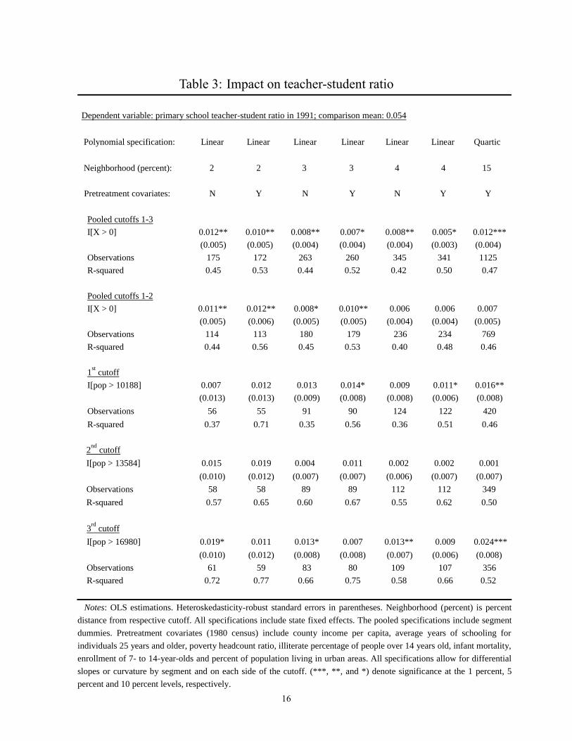
Table 3: Impact on teacher-student ratio
Dependent variable: primary school teacherstudent ratio in 1991; comparison mean: 0.054
Polynomial specification: Linear Linear Linear Linear Linear Linear Quartic
Neighborhood (percent): 2 2 3 3 4 4 15
Pretreatment covariates: N Y N Y N Y Y
Pooled cutoffs 13I[X > 0] 0.012** 0.010** 0.008** 0.007* 0.008** 0.005* 0.012***
(0.005) (0.005) (0.004) (0.004) (0.004) (0.003) (0.004)Observations 175 172 263 260 345 341 1125Rsquared 0.45 0.53 0.44 0.52 0.42 0.50 0.47
Pooled cutoffs 12I[X > 0] 0.011** 0.012** 0.008* 0.010** 0.006 0.006 0.007
(0.005) (0.006) (0.005) (0.005) (0.004) (0.004) (0.005)Observations 114 113 180 179 236 234 769Rsquared 0.44 0.56 0.45 0.53 0.40 0.48 0.46
1st cutoffI[pop > 10188] 0.007 0.012 0.013 0.014* 0.009 0.011* 0.016**
(0.013) (0.013) (0.009) (0.008) (0.008) (0.006) (0.008)Observations 56 55 91 90 124 122 420Rsquared 0.37 0.71 0.35 0.56 0.36 0.51 0.46
2nd cutoffI[pop > 13584] 0.015 0.019 0.004 0.011 0.002 0.002 0.001
(0.010) (0.012) (0.007) (0.007) (0.006) (0.007) (0.007)Observations 58 58 89 89 112 112 349Rsquared 0.57 0.65 0.60 0.67 0.55 0.62 0.50
3rd cutoffI[pop > 16980] 0.019* 0.011 0.013* 0.007 0.013** 0.009 0.024***
(0.010) (0.012) (0.008) (0.008) (0.007) (0.006) (0.008)Observations 61 59 83 80 109 107 356Rsquared 0.72 0.77 0.66 0.75 0.58 0.66 0.52
Notes: OLS estimations. Heteroskedasticityrobust standard errors in parentheses. Neighborhood (percent) is percentdistance from respective cutoff. All specifications include state fixed effects. The pooled specifications include segmentdummies. Pretreatment covariates (1980 census) include county income per capita, average years of schooling forindividuals 25 years and older, poverty headcount ratio, illiterate percentage of people over 14 years old, infant mortality,enrollment of 7 to 14yearolds and percent of population living in urban areas. All specifications allow for differentialslopes or curvature by segment and on each side of the cutoff. (***, **, and *) denote significance at the 1 percent, 5percent and 10 percent levels, respectively.
16

Table5.1:Robustnesschecksforimpactonschooling,19-to28-year-oldsin1991
Dep
ende
nt v
aria
ble:
ave
rage
yea
rs o
f sch
oolin
g, 1
9 to
28
year
old
s in
1991
; com
paris
on m
ean:
4.2
6
Nei
ghbo
rhoo
d (p
erce
nt):
22
23
33
44
4
Popu
latio
n po
lyno
mia
l:Li
near
Qua
drat
icLi
near
Line
arQ
uadr
atic
Line
arLi
near
Qua
drat
icLi
near
Pret
reat
men
tcov
aria
tes:
Line
arN
one
Qua
drat
icLi
near
Non
eQ
uadr
atic
Line
arN
one
Qua
drat
ic
Pool
edcu
toff
s 13
I[X
> 0
]0.
126
0.14
00.
147
0.20
0*0.
152
0.25
4**
0.17
9*0.
386
0.24
8**
(0.1
35)
(0.3
98)
(0.1
60)
(0.1
04)
(0.3
02)
(0.1
15)
(0.0
93)
(0.2
68)
(0.1
00)
Fte
st fo
r H0: γ Y
t1=1
0.30
0.44
0.63
[pv
alue
][0
.58]
[0.5
1][0
.43]
Fte
st fo
rH0:
linea
rity
1.65
1.56
3.86
[pv
alue
][0
.14]
[0.1
6][0
.00]
Fte
st fo
rH0:
linea
rity
0.69
1.28
2.
43[p
val
ue]
[0.6
8][0
.26]
[0.0
2]
Pool
edcu
toff
s 12
I[X
> 0
]0.
085
0.18
40.
150
0.19
90.
222
0.27
6**
0.16
90.
421
0.27
0**
(0.1
62)
(0.5
31)
(0.1
84)
(0.1
28)
(0.3
82)
(0.1
37)
(0.1
18)
(0.3
31)
(0.1
26)
Fte
st fo
r H0: γ Y
t1=1
1.97
1.52
2.05
[pv
alue
][0
.16]
[0.2
2][0
.15]
Fte
st fo
rH0:
linea
rity
1.76
1.39
3.84
[pv
alue
][0
.14]
[0.2
3][0
.00]
Fte
st fo
rH0:
linea
rity
0.50
0.79
1.15
[pv
alue
][0
.83]
[0.6
0][0
.34]
Not
es:O
LS e
stim
atio
ns.H
eter
oske
dast
icity
rob
ust s
tand
ard
erro
rs in
par
enth
eses
. Nei
ghbo
rhoo
d (p
erce
nt) i
spe
rcen
t dis
tanc
e fr
om re
spec
tive
cuto
ff. A
ll sp
ecifi
catio
ns i
nclu
de s
tate
fix
ed e
ffec
ts a
nd s
egm
ent
dum
mie
s. Pr
etre
atm
ent
cova
riate
s (1
980
cens
us)
incl
ude
coun
ty i
ncom
e pe
rca
pita
, ave
rage
yea
rs o
f sch
oolin
g fo
r ind
ivid
uals
25
year
s an
d ol
der,
pove
rty h
eadc
ount
rat
io, i
llite
rate
per
cent
age
of p
eopl
e ov
er 1
4 ye
ars
old,
infa
nt m
orta
lity,
enr
ollm
ent o
f 7 t
o 14
yea
rold
s an
d pe
rcen
t of p
opul
atio
n liv
ing
in u
rban
are
as.C
olum
ns 1
, 4 a
nd 7
als
o in
clud
eav
erag
e ye
ars
ofsc
hool
ing
of th
e 8
to 1
7ye
ars
old
coho
rt in
198
0 (1
9 to
28
year
old
s in
199
1).A
ll sp
ecifi
catio
ns a
llow
for d
iffer
entia
l slo
pes
or c
urva
ture
by
segm
ent a
nd o
n ea
ch si
de o
f the
cut
off.
(***
, **,
and
*) d
enot
e si
gnifi
canc
e at
the
1 pe
rcen
t, 5
perc
ent a
nd 1
0 pe
rcen
t lev
els,
resp
ectiv
ely.
17
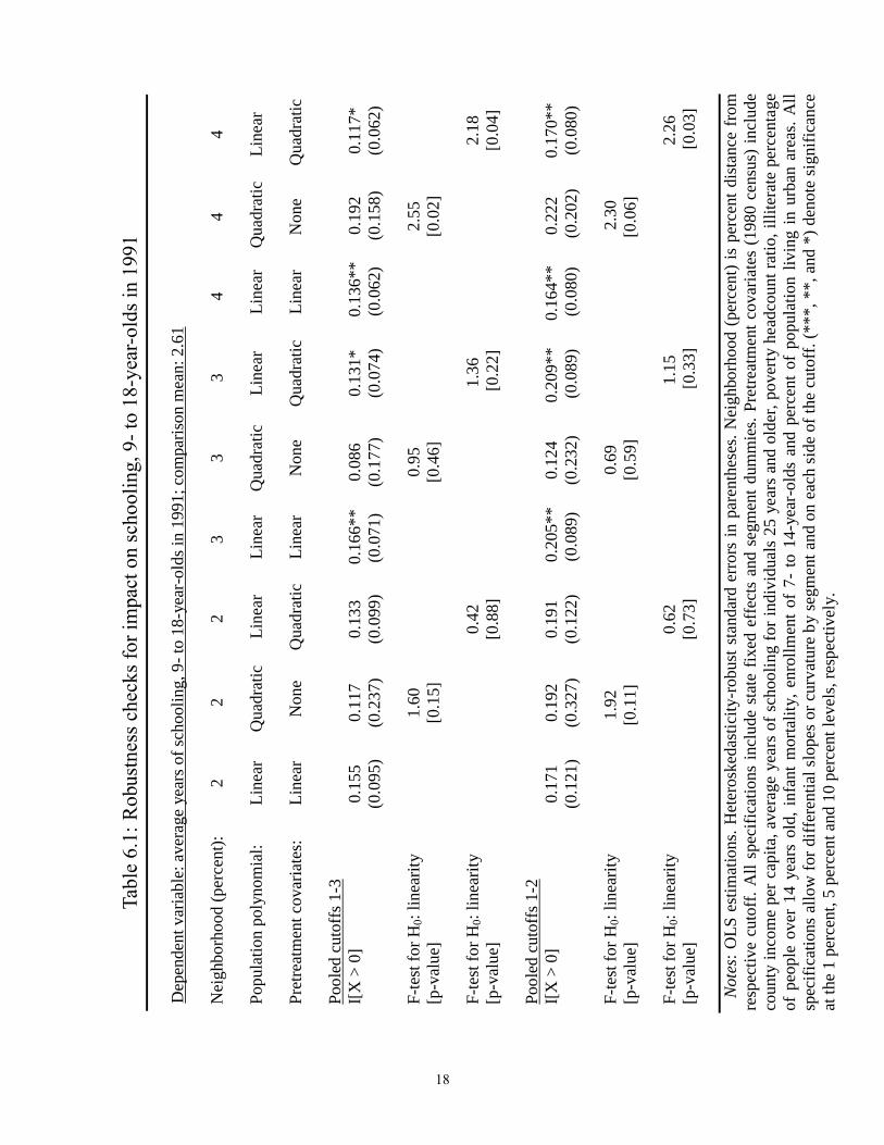
Table6.1:Robustnesschecksforimpactonschooling,9-to18-year-oldsin1991
Dep
ende
nt v
aria
ble:
ave
rage
yea
rs o
f sch
oolin
g, 9
to
18y
ear
olds
in 1
991;
com
paris
onm
ean:
2.6
1
Nei
ghbo
rhoo
d (p
erce
nt):
22
23
33
44
4
Popu
latio
n po
lyno
mia
l:Li
near
Qua
drat
icLi
near
Line
arQ
uadr
atic
Line
arLi
near
Qua
drat
icLi
near
Pret
reat
men
tcov
aria
tes:
Line
arN
one
Qua
drat
icLi
near
Non
eQ
uadr
atic
Line
arN
one
Qua
drat
ic
Pool
edcu
toff
s 13
I[X >
0]
0.15
50.
117
0.13
30.
166*
*0.
086
0.13
1*0.
136*
*0.
192
0.11
7*(0
.095
)(0
.237
)(0
.099
)(0
.071
)(0
.177
)(0
.074
)(0
.062
)(0
.158
)(0
.062
)
Fte
st fo
rH0:
linea
rity
1.60
0.95
2.55
[pv
alue
][0
.15]
[0.4
6][0
.02]
Fte
st fo
rH0:
linea
rity
0.42
1.36
2.1
8[p
val
ue]
[0.8
8][0
.22]
[0.0
4]
Pool
edcu
toff
s 12
I[X >
0]
0.17
10.
192
0.19
10.
205*
*0.
124
0.20
9**
0.16
4**
0.22
20.
170*
*(0
.121
)(0
.327
)(0
.122
)(0
.089
)(0
.232
)(0
.089
) (0
.080
)(0
.202
)(0
.080
)
Fte
st fo
rH0:
linea
rity
1.92
0.69
2.30
[pv
alue
][0
.11]
[0.5
9][0
.06]
Fte
st fo
rH0:
linea
rity
0.62
1.1
52.
26[p
val
ue]
[0.7
3][0
.33]
[0.0
3]
Note
s:O
LS e
stim
atio
ns.H
eter
oske
dast
icity
rob
ust s
tand
ard
erro
rs in
par
enth
eses
. Nei
ghbo
rhoo
d (p
erce
nt) i
spe
rcen
t dis
tanc
e fr
omre
spec
tive
cuto
ff. A
ll sp
ecifi
catio
ns in
clud
e st
ate
fixed
eff
ects
and
seg
men
t dum
mie
s. Pr
etre
atm
ent c
ovar
iate
s (1
980
cens
us)
incl
ude
coun
ty in
com
e pe
r cap
ita, a
vera
ge y
ears
of s
choo
ling
fori
ndiv
idua
ls 2
5 ye
ars
and
olde
r, po
verty
hea
dcou
nt ra
tio, i
llite
rate
per
cent
age
of p
eopl
e ov
er 1
4 ye
ars
old,
infa
nt m
orta
lity,
enr
ollm
ent o
f 7
to 1
4ye
aro
lds
and
perc
ent o
f po
pula
tion
livin
g in
urb
an a
reas
. All
spec
ifica
tions
allo
w fo
r diff
eren
tial s
lope
s or
cur
vatu
re b
y se
gmen
t and
on
each
side
of t
he c
utof
f. (*
**, *
*, a
nd *
) den
ote
sign
ifica
nce
at th
e 1
perc
ent,
5 pe
rcen
t and
10
perc
ent l
evel
s, re
spec
tivel
y.
18
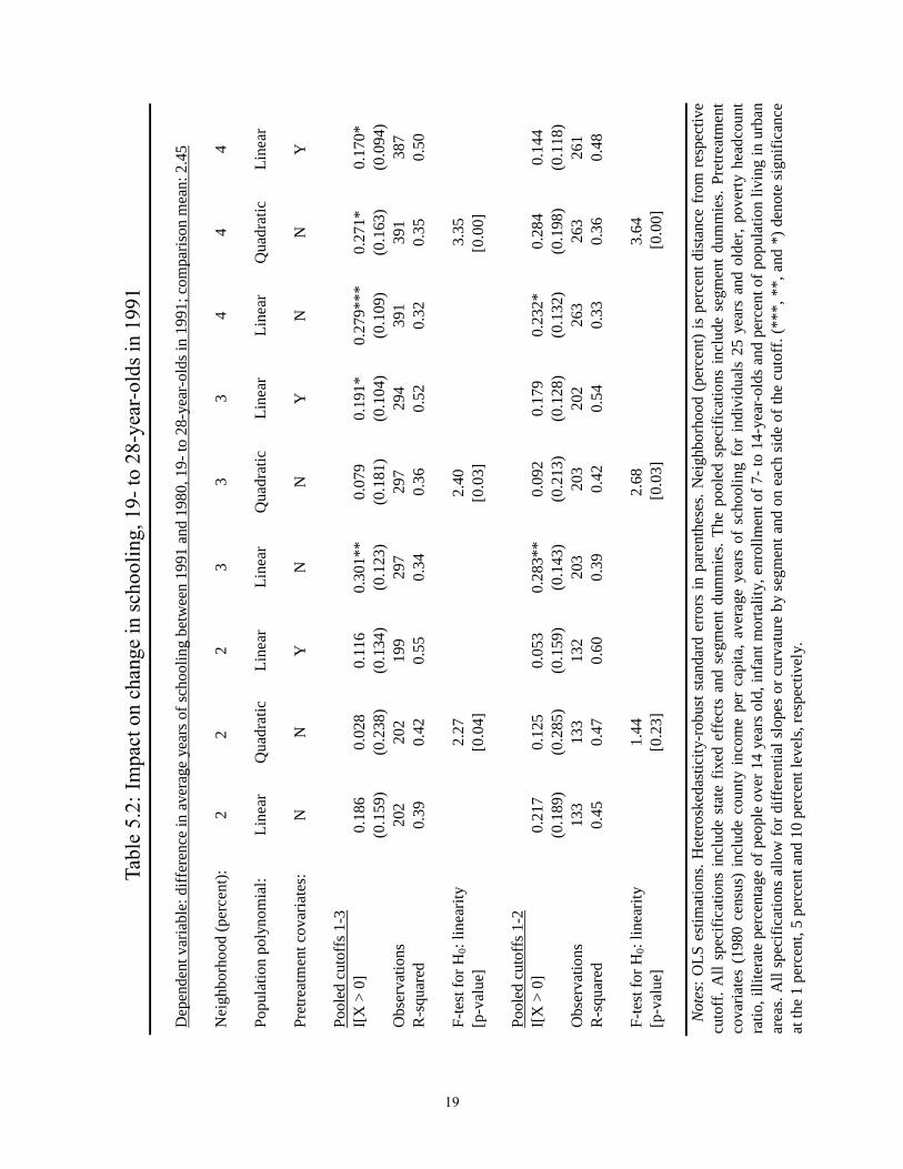
Table5.2:Impactonchangeinschooling,19-to28-year-oldsin1991
Dep
ende
nt v
aria
ble:
diff
eren
ce in
ave
rage
yea
rs o
f sch
oolin
g be
twee
n 19
91 a
nd 1
980,
19
to 2
8ye
aro
lds i
n 19
91;c
ompa
rison
mea
n: 2
.45
Nei
ghbo
rhoo
d (p
erce
nt):
22
23
33
44
4
Popu
latio
n po
lyno
mia
l:Li
near
Qua
drat
icLi
near
Line
arQ
uadr
atic
Line
arLi
near
Qua
drat
icLi
near
Pret
reat
men
t cov
aria
tes:
NN
YN
NY
NN
Y
Pool
edcu
toff
s 13
I[X
> 0
]0.
186
0.02
80.
116
0.30
1**
0.07
90.
191*
0.27
9***
0.27
1*0.
170*
(0.1
59)
(0.2
38)
(0.1
34)
(0.1
23)
(0.1
81)
(0.1
04)
(0.1
09)
(0.1
63)
(0.0
94)
Obs
erva
tions
202
202
199
297
297
294
391
391
387
Rs
quar
ed0.
390.
420.
550.
340.
360.
520.
320.
350.
50
Fte
st fo
rH0:
linea
rity
2.27
2.40
3.35
[pv
alue
][0
.04]
[0.0
3][0
.00]
Pool
edcu
toff
s 12
I[X
> 0
]0.
217
0.12
50.
053
0.28
3**
0.09
20.
179
0.23
2*0.
284
0.14
4(0
.189
)(0
.285
)(0
.159
)(0
.143
)(0
.213
)(0
.128
)(0
.132
)(0
.198
)(0
.118
)O
bser
vatio
ns13
313
313
220
320
320
226
326
326
1R
squ
ared
0.45
0.47
0.60
0.39
0.42
0.54
0.33
0.36
0.48
Fte
st fo
rH0:
linea
rity
1.44
2.68
3.64
[pv
alue
][0
.23]
[0.0
3][0
.00]
Not
es:O
LS e
stim
atio
ns.H
eter
oske
dast
icity
rob
ust s
tand
ard
erro
rs in
par
enth
eses
. Nei
ghbo
rhoo
d (p
erce
nt) i
spe
rcen
t dis
tanc
e fr
om re
spec
tive
cuto
ff.A
ll sp
ecifi
catio
ns in
clud
e st
ate
fixed
eff
ects
and
seg
men
t dum
mie
s. Th
e po
oled
spe
cific
atio
ns in
clud
e se
gmen
t dum
mie
s. Pr
etre
atm
ent
cova
riate
s (1
980
cens
us)
incl
ude
coun
ty in
com
e pe
r ca
pita
, ave
rage
yea
rs o
f sc
hool
ing
for
indi
vidu
als
25 y
ears
and
old
er, p
over
ty h
eadc
ount
ratio
, illi
tera
te p
erce
ntag
e of
peo
ple
over
14
year
s ol
d, in
fant
mor
talit
y, e
nrol
lmen
t of 7
to
14y
ear
olds
and
per
cent
of p
opul
atio
n liv
ing
in u
rban
area
s. A
ll sp
ecifi
catio
ns a
llow
for d
iffer
entia
l slo
pes
or c
urva
ture
by
segm
enta
nd o
n ea
ch s
ide
of th
e cu
toff
.(**
*, *
*, a
nd *
) den
ote
sign
ifica
nce
at th
e 1
perc
ent,
5 pe
rcen
t and
10
perc
ent l
evel
s, re
spec
tivel
y.
19
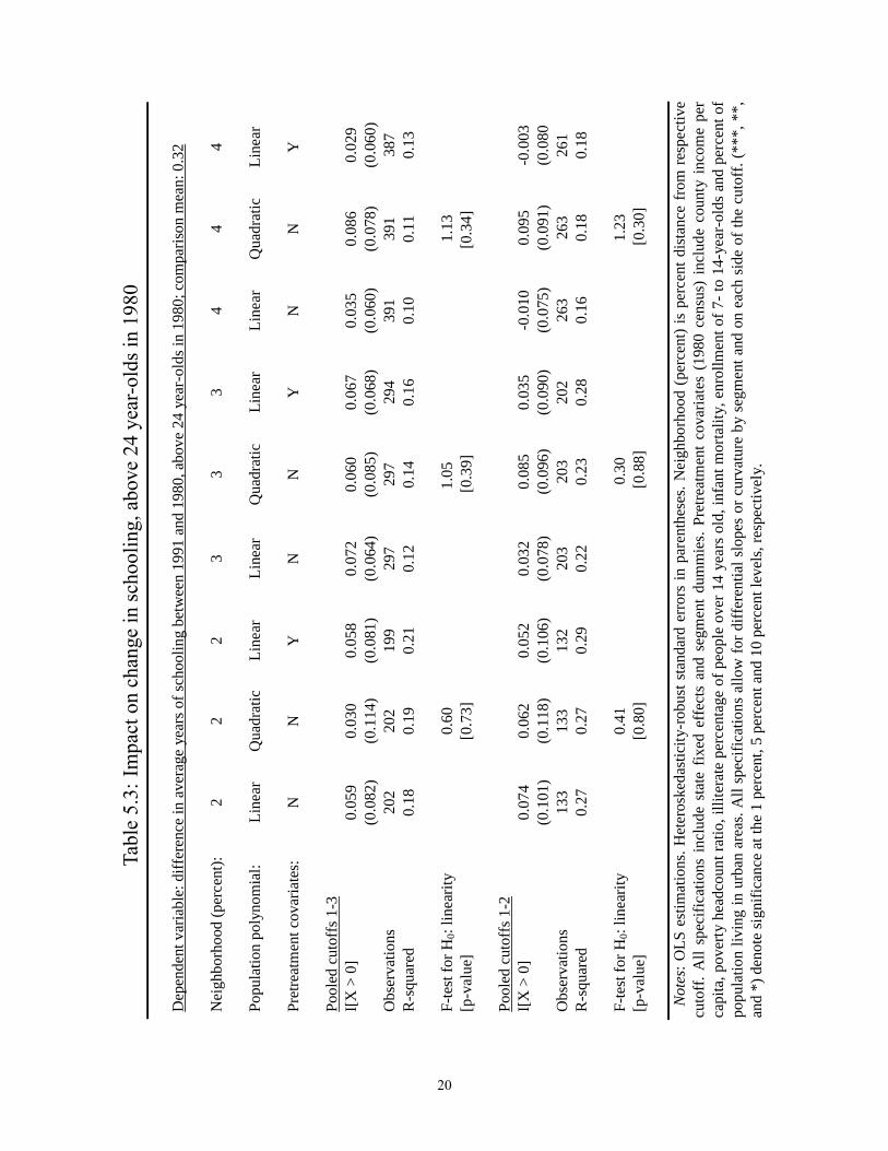
Table5.3:Impactonchangeinschooling,above24year-oldsin1980
Dep
ende
nt v
aria
ble:
diff
eren
ce in
ave
rage
yea
rs o
f sch
oolin
g be
twee
n 19
91 a
nd 1
980,
abo
ve 2
4 ye
aro
lds i
n 19
80; c
ompa
rison
mea
n: 0
.32
Nei
ghbo
rhoo
d (p
erce
nt):
22
23
33
44
4
Popu
latio
n po
lyno
mia
l:Li
near
Qua
drat
icLi
near
Line
arQ
uadr
atic
Line
arLi
near
Qua
drat
icLi
near
Pret
reat
men
t cov
aria
tes:
NN
YN
NY
NN
Y
Pool
edcu
toff
s 13
I[X
> 0
]0.
059
0.03
00.
058
0.07
20.
060
0.06
70.
035
0.08
60.
029
(0.0
82)
(0.1
14)
(0.0
81)
(0.0
64)
(0.0
85)
(0.0
68)
(0.0
60)
(0.0
78)
(0.0
60)
Obs
erva
tions
202
202
199
297
297
294
391
391
387
Rs
quar
ed0.
180.
190.
210.
120.
140.
160.
100.
110.
13
Fte
st fo
rH0:
linea
rity
0.60
1.05
1.13
[pv
alue
][0
.73]
[0.3
9][0
.34]
Pool
edcu
toff
s 12
I[X
> 0
]0.
074
0.06
20.
052
0.03
20.
085
0.03
50
.010
0.09
50
.003
(0.1
01)
(0.1
18)
(0.1
06)
(0.0
78)
(0.0
96)
(0.0
90)
(0.0
75)
(0.0
91)
(0.0
80O
bser
vatio
ns13
313
313
220
320
320
226
326
326
1R
squ
ared
0.27
0.27
0.29
0.22
0.23
0.28
0.16
0.18
0.18
Fte
st fo
rH0:
linea
rity
0.41
0.30
1.23
[pv
alue
][0
.80]
[0.8
8][0
.30]
Not
es:O
LS e
stim
atio
ns.H
eter
oske
dast
icity
rob
ust s
tand
ard
erro
rs in
par
enth
eses
. Nei
ghbo
rhoo
d (p
erce
nt) i
spe
rcen
t dis
tanc
e fr
om re
spec
tive
cuto
ff. A
ll sp
ecifi
catio
ns i
nclu
de s
tate
fix
ed e
ffec
ts a
nd s
egm
ent
dum
mie
s. Pr
etre
atm
ent
cova
riate
s (1
980
cens
us)
incl
ude
coun
ty i
ncom
e pe
rca
pita
, pov
erty
hea
dcou
nt ra
tio, i
llite
rate
per
cent
age
of p
eopl
e ov
er 1
4 ye
ars
old,
infa
nt m
orta
lity,
enr
ollm
ent o
f 7 t
o 14
yea
rol
ds a
nd p
erce
nt o
fpo
pula
tion
livin
g in
urb
an a
reas
. All
spec
ifica
tions
allo
w fo
r diff
eren
tial s
lope
s or
cur
vatu
re b
y se
gmen
t and
on
each
sid
e of
the
cuto
ff. (
***,
**,
and
*) d
enot
e si
gnifi
canc
e at
the
1 pe
rcen
t, 5
perc
ent a
nd 1
0 pe
rcen
t lev
els,
resp
ectiv
ely.
20
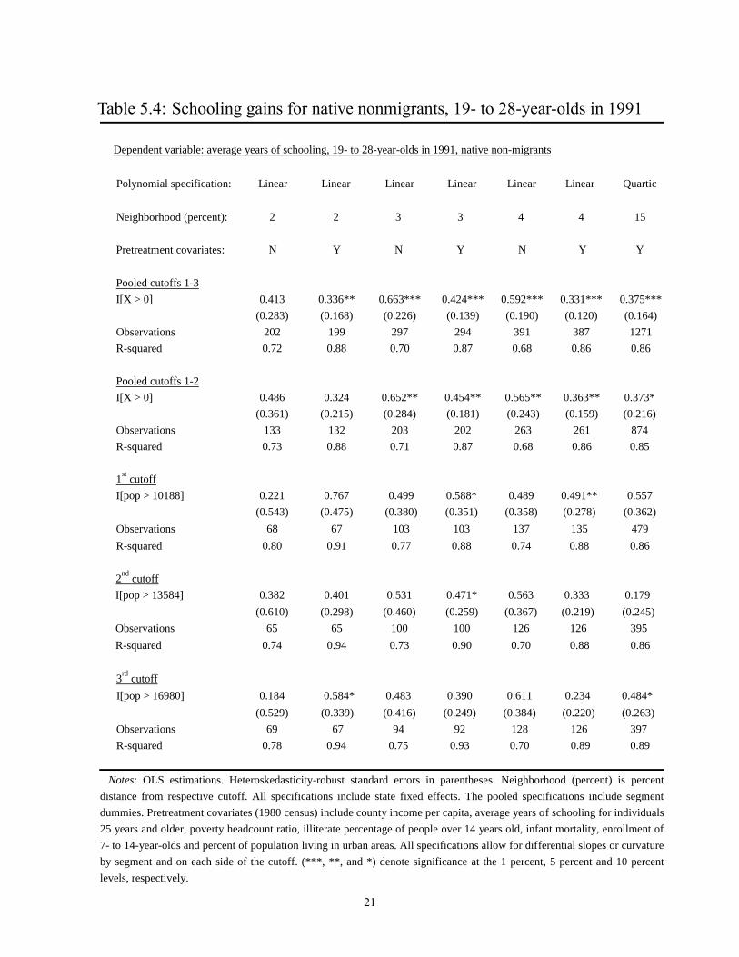
Table 5.4: Schooling gains for native nonmigrants, 19- to 28-year-olds in 1991
Dependent variable: average years of schooling, 19 to 28yearolds in 1991, native nonmigrants
Polynomial specification: Linear Linear Linear Linear Linear Linear Quartic
Neighborhood (percent): 2 2 3 3 4 4 15
Pretreatment covariates: N Y N Y N Y Y
Pooled cutoffs 13I[X > 0] 0.413 0.336** 0.663*** 0.424*** 0.592*** 0.331*** 0.375***
(0.283) (0.168) (0.226) (0.139) (0.190) (0.120) (0.164)Observations 202 199 297 294 391 387 1271Rsquared 0.72 0.88 0.70 0.87 0.68 0.86 0.86
Pooled cutoffs 12I[X > 0] 0.486 0.324 0.652** 0.454** 0.565** 0.363** 0.373*
(0.361) (0.215) (0.284) (0.181) (0.243) (0.159) (0.216)Observations 133 132 203 202 263 261 874Rsquared 0.73 0.88 0.71 0.87 0.68 0.86 0.85
1st cutoffI[pop > 10188] 0.221 0.767 0.499 0.588* 0.489 0.491** 0.557
(0.543) (0.475) (0.380) (0.351) (0.358) (0.278) (0.362)Observations 68 67 103 103 137 135 479Rsquared 0.80 0.91 0.77 0.88 0.74 0.88 0.86
2nd cutoffI[pop > 13584] 0.382 0.401 0.531 0.471* 0.563 0.333 0.179
(0.610) (0.298) (0.460) (0.259) (0.367) (0.219) (0.245)Observations 65 65 100 100 126 126 395Rsquared 0.74 0.94 0.73 0.90 0.70 0.88 0.86
3rd cutoffI[pop > 16980] 0.184 0.584* 0.483 0.390 0.611 0.234 0.484*
(0.529) (0.339) (0.416) (0.249) (0.384) (0.220) (0.263)Observations 69 67 94 92 128 126 397Rsquared 0.78 0.94 0.75 0.93 0.70 0.89 0.89
Notes: OLS estimations. Heteroskedasticityrobust standard errors in parentheses. Neighborhood (percent) is percentdistance from respective cutoff. All specifications include state fixed effects. The pooled specifications include segmentdummies. Pretreatment covariates (1980 census) include county income per capita, average years of schooling for individuals25 years and older, poverty headcount ratio, illiterate percentage of people over 14 years old, infant mortality, enrollment of7 to 14yearolds and percent of population living in urban areas. All specifications allow for differential slopes or curvatureby segment and on each side of the cutoff. (***, **, and *) denote significance at the 1 percent, 5 percent and 10 percentlevels, respectively.
21
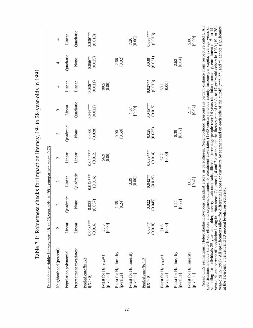
Table7.1:Robustnesschecksforimpactonliteracy,19-to28-year-oldsin1991
Dep
ende
nt v
aria
ble:
lite
racy
rate
, 19
to 2
8ye
aro
lds i
n 19
91,c
ompa
rison
mea
n: 0
.76
Nei
ghbo
rhoo
d (p
erce
nt):
22
23
33
44
4
Popu
latio
n po
lyno
mia
l:Li
near
Qua
drat
icLi
near
Line
arQ
uadr
atic
Line
arLi
near
Qua
drat
icLi
near
Pret
reat
men
tcov
aria
tes:
Line
arN
one
Qua
drat
icLi
near
Non
eQ
uadr
atic
Line
arN
one
Qua
drat
ic
Pool
edcu
toffs
13
I[X >
0]
0.0
43**
*
0.0
33 0
.042
***
0.04
4***
0.03
80.
044*
** 0
.036
** 0
.056
**0.
036*
**
(0.0
16)
(0
.037
)
(0.0
16)
(0.0
12)
(0.0
28)
(0.
012)
(0.0
11)
(0.0
25)
(0.0
10)
Fte
st fo
r H0: γ Y
t1=1
35.5
56.9
80.5
[pv
alue
][0
.00]
[0.0
0][0
.00]
Fte
st fo
r H0:
linea
rity
1.35
0.90
2.6
6[p
val
ue]
[0.2
4][0
.50]
[0.0
2]
Fte
st fo
r H0:
linea
rity
3.39
4.07
7
.26
[pv
alue
][0
.00]
[0.0
0][0
.00]
Pool
ed c
utof
fs 1
2I[X
> 0
]
0.0
34*
0.02
20.
042*
* 0
.039
***
0.02
80.
045*
**0.
027*
*0.
038
0.03
3***
(0
.018
)(0
.045
)(0
.019
) (0
.014
)(0
.035
)(0
.015
)(0
.013
)(0
.031
)(0
.013
)
Fte
st fo
r H0: γ Y
t1=1
21.6
57.7
50.1
[pv
alue
][0
.00]
[0.0
0][0
.00]
Fte
st fo
r H0:
linea
rity
1.4
4
0.39
2.62
[pv
alue
][0
.22]
[0.8
2][0
.04]
Fte
st fo
r H0:
linea
rity
1
.03
2.
17
5.80
[pv
alue
][0
.41]
[0.0
4][0
.00]
Not
es:O
LS e
stim
atio
ns.H
eter
oske
dast
icity
robu
st s
tand
ard
erro
rs in
par
enth
eses
. Nei
ghbo
rhoo
d (p
erce
nt)
ispe
rcen
t dist
ance
fro
m r
espe
ctiv
e cu
toff
. All
spec
ifica
tions
incl
ude
state
fix
ed e
ffec
ts a
nd s
egm
ent d
umm
ies.
Pret
reat
men
t cov
aria
tes
(198
0 ce
nsus
) in
clud
e co
unty
inco
me
per
capi
ta, a
vera
ge y
ears
of
scho
olin
g fo
r ind
ivid
uals
25
year
s an
d ol
der,
pove
rty h
eadc
ount
ratio
,illi
tera
te p
erce
ntag
e pe
ople
ove
r 14
year
s ol
d, in
fant
mor
talit
y, e
nrol
lmen
t of 7
to
14
year
old
s an
d pe
rcen
t of p
opul
atio
n liv
ing
in u
rban
are
as.C
olum
ns 1
, 4 a
nd 7
als
o in
clud
e th
e lit
erac
y ra
te o
f the
8 t
o 17
yea
rso
ld c
ohor
t in
1980
(19
to 2
8ye
aro
lds
in 1
991)
.All
spec
ifica
tions
allo
w fo
r diff
eren
tial s
lope
s or
cur
vatu
re b
y se
gmen
t and
on
each
sid
e of
the
cuto
ff. (
***,
**,
and
*) d
enot
e si
gnifi
canc
eat
the
1 pe
rcen
t, 5
perc
ent a
nd 1
0 pe
rcen
t lev
els,
resp
ectiv
ely.
22
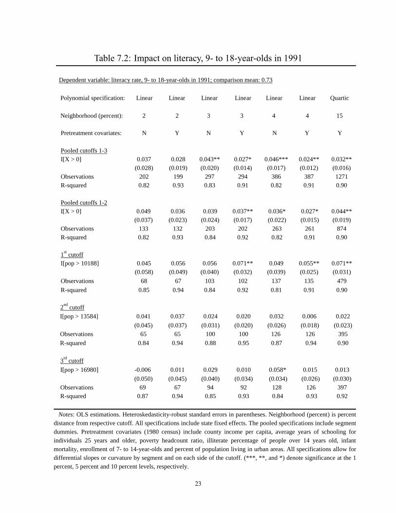
Table 7.2: Impact on literacy, 9- to 18-year-olds in 1991
Dependent variable: literacy rate, 9 to 18yearolds in 1991; comparison mean: 0.73
Polynomial specification: Linear Linear Linear Linear Linear Linear Quartic
Neighborhood (percent): 2 2 3 3 4 4 15
Pretreatment covariates: N Y N Y N Y Y
Pooled cutoffs 13I[X > 0] 0.037 0.028 0.043** 0.027* 0.046*** 0.024** 0.032**
(0.028) (0.019) (0.020) (0.014) (0.017) (0.012) (0.016)Observations 202 199 297 294 386 387 1271Rsquared 0.82 0.93 0.83 0.91 0.82 0.91 0.90
Pooled cutoffs 12I[X > 0] 0.049 0.036 0.039 0.037** 0.036* 0.027* 0.044**
(0.037) (0.023) (0.024) (0.017) (0.022) (0.015) (0.019)Observations 133 132 203 202 263 261 874Rsquared 0.82 0.93 0.84 0.92 0.82 0.91 0.90
1st cutoffI[pop > 10188] 0.045 0.056 0.056 0.071** 0.049 0.055** 0.071**
(0.058) (0.049) (0.040) (0.032) (0.039) (0.025) (0.031)Observations 68 67 103 102 137 135 479Rsquared 0.85 0.94 0.84 0.92 0.81 0.91 0.90
2nd cutoffI[pop > 13584] 0.041 0.037 0.024 0.020 0.032 0.006 0.022
(0.045) (0.037) (0.031) (0.020) (0.026) (0.018) (0.023)Observations 65 65 100 100 126 126 395Rsquared 0.84 0.94 0.88 0.95 0.87 0.94 0.90
3rd cutoffI[pop > 16980] 0.006 0.011 0.029 0.010 0.058* 0.015 0.013
(0.050) (0.045) (0.040) (0.034) (0.034) (0.026) (0.030)Observations 69 67 94 92 128 126 397Rsquared 0.87 0.94 0.85 0.93 0.84 0.93 0.92
Notes: OLS estimations. Heteroskedasticityrobust standard errors in parentheses. Neighborhood (percent) is percentdistance from respective cutoff. All specifications include state fixed effects. The pooled specifications include segmentdummies. Pretreatment covariates (1980 census) include county income per capita, average years of schooling forindividuals 25 years and older, poverty headcount ratio, illiterate percentage of people over 14 years old, infantmortality, enrollment of 7 to 14yearolds and percent of population living in urban areas. All specifications allow fordifferential slopes or curvature by segment and on each side of the cutoff. (***, **, and *) denote significance at the 1percent, 5 percent and 10 percent levels, respectively.
23
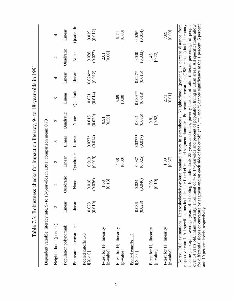
Table7.3:Robustnesschecksforimpactonliteracy,9-to18-year-oldsin1991
Dep
ende
nt v
aria
ble:
lite
racy
rate
, 9 t
o 18
yea
rol
ds in
199
1; c
ompa
rison
mea
n: 0
.73
Nei
ghbo
rhoo
d (p
erce
nt):
22
23
33
44
4
Popu
latio
n po
lyno
mia
l:Li
near
Qua
drat
icLi
near
Line
arQ
uadr
atic
Line
arLi
near
Qua
drat
icLi
near
Pret
reat
men
tcov
aria
tes:
Line
arN
one
Qua
drat
icLi
near
Non
eQ
uadr
atic
Line
arN
one
Qua
drat
ic
Pool
edcu
toff
s 13
I[X
> 0
]0.
028
0.01
80.
019
0.02
7*0.
016
0.02
10.
024*
* 0
.028
0.01
9(0
.019
)(0
.036
)(0
.019
)(0
.014
)(0
.029
)(0
.014
)(0
.012
)(0
.027
)(0
.012
)
Fte
st fo
rH0:
linea
rity
1.68
0.91
2.01
[pv
alue
][0
.13]
[0.5
0][0
.06]
Fte
st fo
rH0:
linea
rity
4.38
5.69
9
.74
[pv
alue
][0
.00]
[0.0
0][0
.00]
Pool
edcu
toff
s 12
I[X
> 0
]0.
036
0.02
40.
037
0.03
7**
0.02
10.
039*
*0.
027*
0.03
00.
026*
(0.0
23)
(0.0
46)
(0.0
25)
(0.0
17)
(0.0
36)
(0.0
18)
(0.0
15)
(0.0
33)
(0.0
14)
Fte
st fo
rH0:
linea
rity
2.03
0.81
1.43
[pv
alue
][0
.10]
[0.5
2][0
.22]
Fte
st fo
rH0:
linea
rity
1.09
2
.71
7.09
[pv
alue
][0
.37]
[0.0
1][0
.00]
Not
es:
OLS
est
imat
ions
.H
eter
oske
dast
icity
rob
ust
stan
dard
err
ors
in p
aren
thes
es.
Nei
ghbo
rhoo
d (p
erce
nt)
ispe
rcen
t di
stan
ce f
rom
resp
ectiv
e cu
toff
. All
spec
ifica
tions
incl
ude
stat
e fix
ed e
ffec
ts a
nd s
egm
ent d
umm
ies.
Pret
reat
men
t cov
aria
tes (
1980
cen
sus)
incl
ude
coun
tyin
com
e pe
r ca
pita
, ave
rage
yea
rs o
f sc
hool
ing
for
indi
vidu
als
25 y
ears
and
old
er, p
over
ty h
eadc
ount
rat
io, i
llite
rate
per
cent
age
of p
eopl
eov
er 1
4 ye
ars o
ld, i
nfan
t mor
talit
y, e
nrol
lmen
t of 7
to
14y
earo
lds
and
perc
ent o
f pop
ulat
ion
livin
g in
urb
an a
reas
. All
spec
ifica
tions
allo
wfo
r diff
eren
tial s
lope
s or c
urva
ture
by
segm
ent a
ndon
eac
h si
de o
f the
cut
off.
(***
, **,
and
*) d
enot
e si
gnifi
canc
e at
the
1 pe
rcen
t, 5
perc
ent
and
10 p
erce
nt le
vels
, res
pect
ivel
y.
24
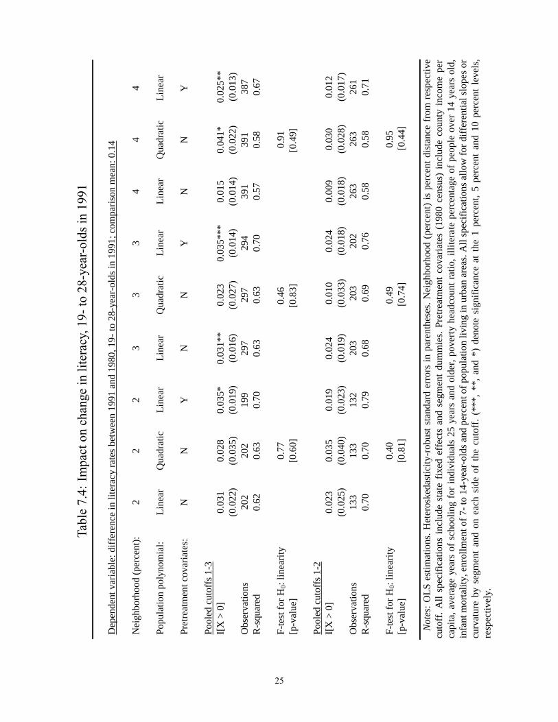
Table7.4:Impactonchangeinliteracy,19-to28-year-oldsin1991
Dep
ende
nt v
aria
ble:
diff
eren
ce in
lite
racy
rate
s bet
wee
n 19
91 a
nd 1
980,
19
to 2
8ye
aro
lds i
n 19
91; c
ompa
rison
mea
n: 0
.14
Nei
ghbo
rhoo
d (p
erce
nt):
22
23
33
44
4
Popu
latio
n po
lyno
mia
l:Li
near
Qua
drat
icLi
near
Line
arQ
uadr
atic
Line
arLi
near
Qua
drat
icLi
near
Pret
reat
men
t cov
aria
tes:
NN
YN
NY
NN
Y
Pool
edcu
toff
s 13
I[X
> 0
]0.
031
0.02
80.
035*
0.03
1**
0.02
30.
035*
**0.
015
0.04
1*0.
025*
*(0
.022
)(0
.035
)(0
.019
)(0
.016
)(0
.027
)(0
.014
)(0
.014
)(0
.022
)(0
.013
)O
bser
vatio
ns20
220
219
929
729
729
439
139
138
7R
squ
ared
0.62
0.63
0.70
0.63
0.63
0.70
0.57
0.58
0.67
Fte
st fo
rH0:
linea
rity
0.77
0.46
0.91
[pv
alue
][0
.60]
[0.8
3][0
.49]
Pool
edcu
toff
s 12
I[X
> 0
]0.
023
0.03
50.
019
0.02
40.
010
0.02
40.
009
0.03
00.
012
(0.0
25)
(0.0
40)
(0.0
23)
(0.0
19)
(0.0
33)
(0.0
18)
(0.0
18)
(0.0
28)
(0.0
17)
Obs
erva
tions
133
133
132
203
203
202
263
263
261
Rs
quar
ed0.
700.
700.
790.
680.
690.
760.
580.
580.
71
Fte
st fo
rH0:
linea
rity
0.40
0.49
0.95
[pv
alue
][0
.81]
[0.7
4][0
.44]
Not
es: O
LS e
stim
atio
ns. H
eter
oske
dast
icity
rob
ust s
tand
ard
erro
rs in
par
enth
eses
. Nei
ghbo
rhoo
d (p
erce
nt) i
spe
rcen
t dis
tanc
e fr
om re
spec
tive
cuto
ff. A
ll sp
ecifi
catio
ns i
nclu
de s
tate
fix
ed e
ffec
ts a
nd s
egm
ent
dum
mie
s. Pr
etre
atm
ent c
ovar
iate
s (1
980
cens
us)
incl
ude
coun
ty in
com
e pe
rca
pita
, ave
rage
yea
rs o
f sch
oolin
g fo
r ind
ivid
uals
25
year
s an
d ol
der,
pove
rty h
eadc
ount
ratio
, illi
tera
te p
erce
ntag
e of
peo
ple
over
14
year
s ol
d,in
fant
mor
talit
y, e
nrol
lmen
t of 7
to
14y
ear
olds
and
per
cent
of p
opul
atio
n liv
ing
in u
rban
are
as. A
ll sp
ecifi
catio
ns a
llow
for d
iffer
entia
l slo
pes o
rcu
rvat
ure
by s
egm
ent
and
on e
ach
side
of
the
cuto
ff.(
***,
**,
and
*)
deno
te s
igni
fican
ce a
t th
e 1
perc
ent,
5 pe
rcen
t an
d 10
per
cent
lev
els,
resp
ectiv
ely.
25

Table 7.5: Literacy gains for native nonmigrants, 19- to 28-year-olds in 1991
Dependent variable: literacy rate, 19 to 28yearolds in 1991, native nonmigrants
Polynomial specification: Linear Linear Linear Linear Linear Linear Quartic
Neighborhood (percent): 2 2 3 3 4 4 15
Pretreatment covariates: N Y N Y N Y Y
Pooled cutoffs 13I[X > 0] 0.065** 0.055*** 0.076*** 0.061*** 0.062*** 0.044*** 0.055***
(0.028) (0.017) (0.022) (0.015) (0.018) (0.012) (0.016)Observations 202 199 297 294 391 387 1271Rsquared 0.77 0.91 0.77 0.89 0.78 0.89 0.88
Pooled cutoffs 12I[X > 0] 0.058 0.047** 0.058** 0.060*** 0.044** 0.036** 0.050**
(0.037) (0.020) (0.026) (0.017) (0.022) (0.015) (0.020)Observations 133 132 203 202 263 261 874Rsquared 0.77 0.93 0.79 0.90 0.79 0.89 0.88
1st cutoffI[pop > 10188] 0.060 0.085** 0.058 0.087*** 0.038 0.045* 0.070**
(0.061) (0.036) (0.042) (0.027) (0.040) (0.026) (0.030)Observations 68 67 103 102 137 135 479Rsquared 0.81 0.95 0.82 0.94 0.81 0.92 0.89
2nd cutoffI[pop > 13584] 0.035 0.023 0.048 0.046* 0.049* 0.029 0.029
(0.044) (0.025) (0.038) (0.027) (0.028) (0.020) (0.025)Observations 65 65 100 100 126 126 395Rsquared 0.82 0.95 0.81 0.89 0.82 0.89 0.88
3rd cutoffI[pop > 16980] 0.062 0.055* 0.081** 0.057* 0.080** 0.038* 0.065**
(0.046) (0.033) (0.038) (0.029) (0.033) (0.023) (0.029)Observations 69 67 94 92 128 126 397Rsquared 0.86 0.94 0.84 0.93 0.82 0.93 0.90
Notes: OLS estimations. Heteroskedasticityrobust standard errors in parentheses. Neighborhood (percent) is percentdistance from respective cutoff. All specifications include state fixed effects. The pooled specifications include segmentdummies. Pretreatment covariates (1980 census) include county income per capita, average years of schooling forindividuals 25 years and older, poverty headcount ratio, illiterate percentage of people over 14 years old, infant mortality,enrollment of 7 to 14yearolds and percent of population living in urban areas. All specifications allow for differentialslopes or curvature by segment and on each side of the cutoff. (***, **, and *) denote significance at the 1 percent, 5percent and 10 percent levels, respectively.
26
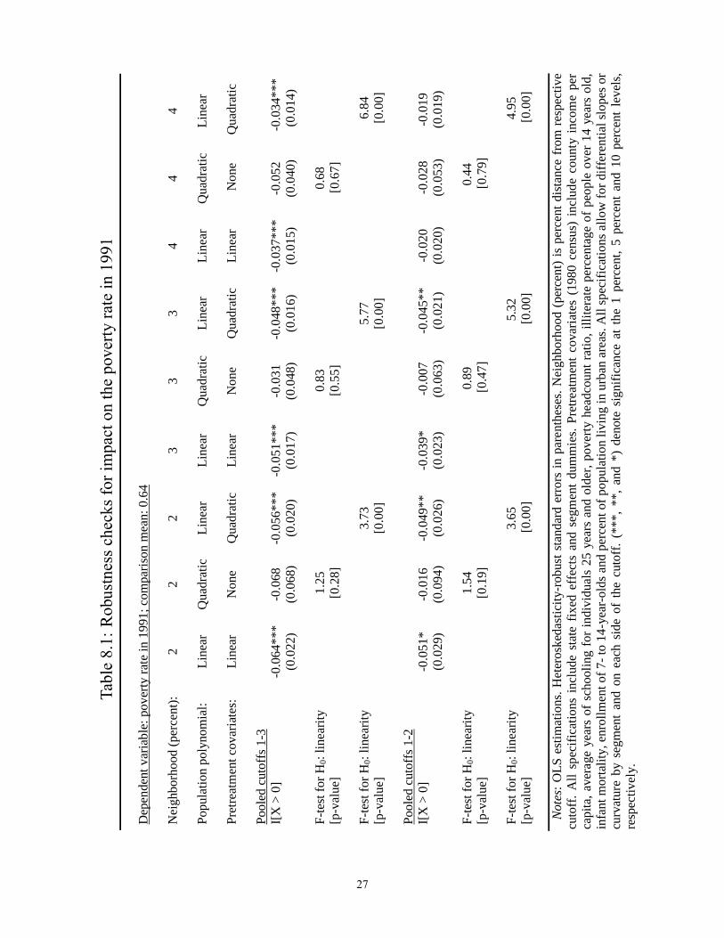
Table8.1:Robustnesschecksforimpactonthepovertyratein1991
Dep
ende
nt v
aria
ble:
pove
rty ra
te in
1991
; com
paris
onm
ean:
0.6
4
Nei
ghbo
rhoo
d (p
erce
nt):
22
23
33
44
4
Popu
latio
n po
lyno
mia
l:Li
near
Qua
drat
icLi
near
Line
arQ
uadr
atic
Line
arLi
near
Qua
drat
icLi
near
Pret
reat
men
tcov
aria
tes:
Line
arN
one
Qua
drat
icLi
near
Non
eQ
uadr
atic
Line
arN
one
Qua
drat
ic
Pool
edcu
toff
s 13
I[X
> 0
]0
.064
***
0.0
680
.056
***
0.0
51**
*0
.031
0.0
48**
*0
.037
***
0.0
520
.034
***
(0.0
22)
(0.0
68)
(0.0
20)
(0.0
17)
(0.0
48)
(0.0
16)
(0.0
15)
(0.0
40)
(0.0
14)
Fte
st fo
r H0:
linea
rity
1.2
5
0
.83
0.68
[pv
alue
][0
.28]
[0.5
5][0
.67]
Fte
st fo
r H0:
linea
rity
3.73
5.77
6.84
[pv
alue
][0
.00]
[0.0
0][0
.00]
Pool
edcu
toff
s 12
I[X
> 0
]0
.051
*0
.016
0.0
49**
0.0
39*
0.0
070
.045
**0
.020
0.0
280
.019
(0.0
29)
(0.0
94)
(0.0
26)
(0.0
23)
(0.0
63)
(0.0
21)
(0.0
20)
(0.0
53)
(0.0
19)
Fte
st fo
r H0:
linea
rity
1.5
4
0.89
0.44
[pv
alue
][0
.19]
[0.4
7][0
.79]
Fte
st fo
r H0:
linea
rity
3.65
5.32
4.95
[pv
alue
][0
.00]
[0.0
0][0
.00]
Note
s:O
LS e
stim
atio
ns.H
eter
oske
dast
icity
rob
ust s
tand
ard
erro
rs in
par
enth
eses
. Nei
ghbo
rhoo
d (p
erce
nt) i
spe
rcen
t dis
tanc
e fr
om re
spec
tive
cuto
ff. A
ll sp
ecifi
catio
ns i
nclu
de s
tate
fix
ed e
ffec
ts a
nd s
egm
ent
dum
mie
s. Pr
etre
atm
ent
cova
riate
s (1
980
cens
us)
incl
ude
coun
ty in
com
e pe
rca
pita
, ave
rage
yea
rs o
f sch
oolin
g fo
r ind
ivid
uals
25
year
s an
d ol
der,
pove
rty h
eadc
ount
ratio
, illi
tera
te p
erce
ntag
e of
peo
ple
over
14
year
s ol
d,in
fant
mor
talit
y, e
nrol
lmen
t of 7
to
14y
earo
lds a
nd p
erce
nt o
f pop
ulat
ion
livin
g in
urb
an a
reas
. All
spec
ifica
tions
allo
w fo
r diff
eren
tial s
lope
s or
curv
atur
e by
seg
men
t an
d on
eac
h si
de o
f th
e cu
toff
. (**
*, *
*, a
nd *
) de
note
sig
nific
ance
at
the
1 pe
rcen
t, 5
perc
ent a
nd 1
0 pe
rcen
t le
vels
,re
spec
tivel
y.
27
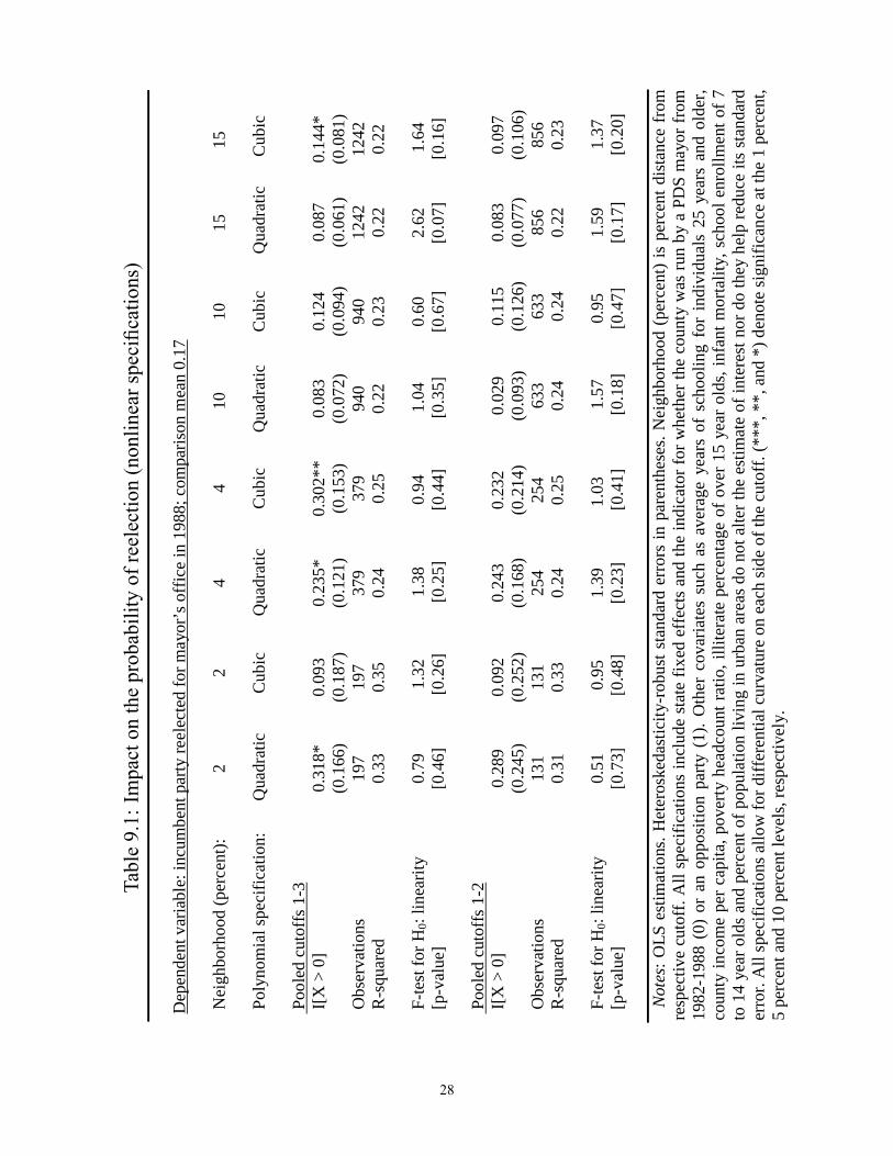
Table9.1:Impactontheprobabilityofreelection(nonlinearspeci�cations)
Dep
ende
ntva
riabl
e:in
cum
bent
par
ty re
elec
ted
for m
ayor
’s o
ffic
e in
198
8;co
mpa
rison
mea
n0.
17
Nei
ghbo
rhoo
d (p
erce
nt):
2 2
4
410
1015
15
Poly
nom
ial s
peci
ficat
ion:
Qua
drat
ic C
ubic
Qua
drat
icC
ubic
Qua
drat
icC
ubic
Qua
drat
icC
ubic
Pool
edcu
toffs
13
I[X
> 0
]0.
318*
0.09
30.
235*
0.30
2**
0.08
30.
124
0.08
70.
144*
(0.1
66)
(0.1
87)
(0.1
21)
(0.1
53)
(0.0
72)
(0.0
94)
(0.0
61)
(0.0
81)
Obs
erva
tions
197
197
379
379
940
940
1242
1242
Rs
quar
ed0.
330.
350.
240.
250.
220.
230.
220.
22
Fte
st fo
r H0:
linea
rity
0.79
1.32
1.3
8 0
.94
1.04
0.60
2.62
1.64
[pv
alue
][0
.46]
[0.2
6] [0
.25]
[0.4
4][0
.35]
[0.6
7][0
.07]
[0
.16]
Pool
edcu
toffs
12
I[X
> 0
]0.
289
0.09
20.
243
0.23
20.
029
0.11
50.
083
0.09
7(0
.245
)(0
.252
)(0
.168
)(0
.214
)(0
.093
)(0
.126
)(0
.077
)(0
.106
)O
bser
vatio
ns13
113
125
425
463
363
385
685
6R
squ
ared
0.31
0.33
0.24
0.25
0.24
0.24
0.22
0.23
Fte
st fo
r H0:
linea
rity
0.51
0.95
1.39
1.03
1.57
0.95
1.59
1.37
[pv
alue
][0
.73]
[0.4
8][0
.23]
[0.4
1][0
.18]
[0.4
7][0
.17]
[0.2
0]
Note
s:O
LS e
stim
atio
ns.H
eter
oske
dast
icity
rob
ust s
tand
ard
erro
rs in
par
enth
eses
. Nei
ghbo
rhoo
d (p
erce
nt) i
spe
rcen
t dis
tanc
e fr
omre
spec
tive
cuto
ff. A
llsp
ecifi
catio
ns in
clud
e st
ate
fixed
eff
ects
and
the
indi
cato
r for
whe
ther
the
coun
ty w
as ru
n by
a P
DS
may
or fr
om19
821
988
(0)
or a
n op
posi
tion
party
(1)
. Oth
er c
ovar
iate
s su
ch a
s av
erag
e ye
ars
of s
choo
ling
for
indi
vidu
als
25 y
ears
and
old
er,
coun
ty in
com
epe
r cap
ita, p
over
ty h
eadc
ount
ratio
, illi
tera
te p
erce
ntag
e of
ove
r 15
year
old
s, in
fant
mor
talit
y,sc
hool
enro
llmen
t of 7
to 1
4 ye
ar o
lds
and
perc
ent o
f pop
ulat
ion
livin
g in
urb
an a
reas
do
not a
lter t
he e
stim
ate
of in
tere
stno
r do
they
hel
p re
duce
its
stan
dard
erro
r. A
ll sp
ecifi
catio
ns a
llow
for d
iffer
entia
lcur
vatu
re o
n ea
ch si
de o
f the
cut
off.
(***
, **,
and
*) d
enot
e si
gnifi
canc
e at
the
1 pe
rcen
t,5
perc
ent a
nd 1
0 pe
rcen
t lev
els,
resp
ectiv
ely.
28
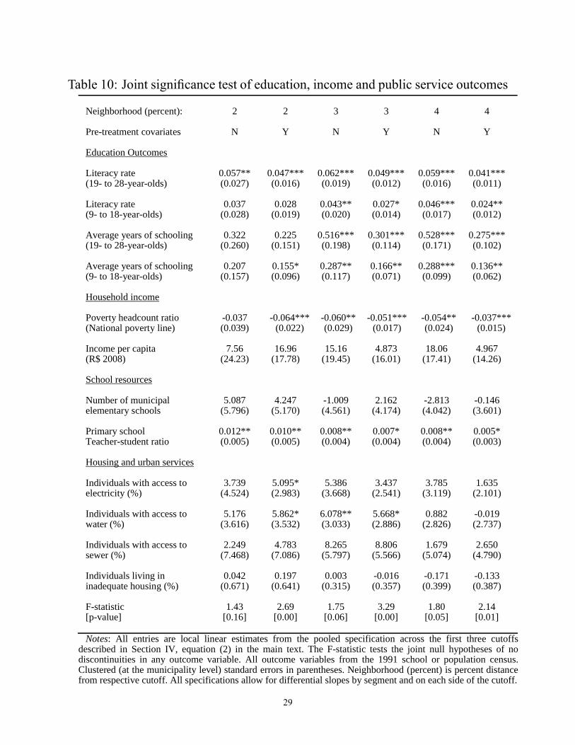
Table 10: Joint signi�cance test of education, income and public service outcomes
Neighborhood (percent): 2 2 3 3 4 4
Pretreatment covariates
Education Outcomes
N Y N Y N Y
Literacy rate 0.057** 0.047*** 0.062*** 0.049*** 0.059*** 0.041***(19 to 28yearolds) (0.027) (0.016) (0.019) (0.012) (0.016) (0.011)
Literacy rate 0.037 0.028 0.043** 0.027* 0.046*** 0.024**(9 to 18yearolds) (0.028) (0.019) (0.020) (0.014) (0.017) (0.012)
Average years of schooling 0.322 0.225 0.516*** 0.301*** 0.528*** 0.275***(19 to 28yearolds) (0.260) (0.151) (0.198) (0.114) (0.171) (0.102)
Average years of schooling 0.207 0.155* 0.287** 0.166** 0.288*** 0.136**(9 to 18yearolds) (0.157) (0.096) (0.117) (0.071) (0.099) (0.062)
Household income
Poverty headcount ratio 0.037 0.064*** 0.060** 0.051*** 0.054** 0.037***(National poverty line) (0.039) (0.022) (0.029) (0.017) (0.024) (0.015)
Income per capita 7.56 16.96 15.16 4.873 18.06 4.967(R$ 2008) (24.23) (17.78) (19.45) (16.01) (17.41) (14.26)
School resources
Number of municipal 5.087 4.247 1.009 2.162 2.813 0.146elementary schools (5.796) (5.170) (4.561) (4.174) (4.042) (3.601)
Primary school 0.012** 0.010** 0.008** 0.007* 0.008** 0.005*Teacherstudent ratio
Housing and urban services
(0.005) (0.005) (0.004) (0.004) (0.004) (0.003)
Individuals with access to 3.739 5.095* 5.386 3.437 3.785 1.635electricity (%) (4.524) (2.983) (3.668) (2.541) (3.119) (2.101)
Individuals with access to 5.176 5.862* 6.078** 5.668* 0.882 0.019water (%) (3.616) (3.532) (3.033) (2.886) (2.826) (2.737)
Individuals with access to 2.249 4.783 8.265 8.806 1.679 2.650sewer (%) (7.468) (7.086) (5.797) (5.566) (5.074) (4.790)
Individuals living in 0.042 0.197 0.003 0.016 0.171 0.133inadequate housing (%) (0.671) (0.641) (0.315) (0.357) (0.399) (0.387)
Fstatistic 1.43 2.69 1.75 3.29 1.80 2.14[pvalue] [0.16] [0.00] [0.06] [0.00] [0.05] [0.01]
Notes: All entries are local linear estimates from the pooled specification across the first three cutoffsdescribed in Section IV, equation (2) in the main text. The Fstatistic tests the joint null hypotheses of nodiscontinuities in any outcome variable. All outcome variables from the 1991 school or population census.Clustered (at the municipality level) standard errors in parentheses. Neighborhood (percent) is percent distancefrom respective cutoff. All specifications allow for differential slopes by segment and on each side of the cutoff.
29
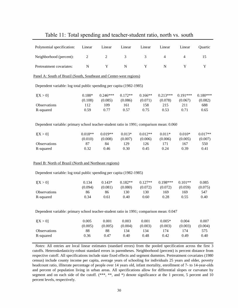
Table 11: Total spending and teacher-student ratio, north vs. south
Polynomial specification: Linear Linear Linear Linear Linear Linear Quartic
Neighborhood (percent): 2 2 3 3 4 4 15
Pretreatment covariates: N Y N Y N Y Y
Panel A: South of Brazil (South, Southeast and Centerwest regions)
Dependent variable: log total public spending per capita (19821985)
I[X > 0] 0.188* 0.246*** 0.172** 0.166** 0.213*** 0.191*** 0.180***(0.108) (0.085) (0.086) (0.071) (0.078) (0.067) (0.082)
Observations 112 109 161 158 215 211 688Rsquared 0.59 0.77 0.57 0.75 0.53 0.71 0.65
Dependent variable: primary school teacherstudent ratio in 1991; comparison mean: 0.060
I[X > 0] 0.018** 0.019** 0.013* 0.012** 0.011* 0.010* 0.017**(0.010) (0.008) (0.007) (0.006) (0.006) (0.005) (0.007)
Observations 87 84 129 126 171 167 550Rsquared 0.32 0.46 0.30 0.45 0.24 0.39 0.41
Panel B: North of Brazil (North and Northeast regions)
Dependent variable: log total public spending per capita (19821985)
I[X > 0] 0.134 0.143* 0.182** 0.127** 0.198*** 0.101** 0.085(0.094) (0.081) (0.080) (0.072) (0.072) (0.059) (0.075)
Observations 86 86 130 130 169 169 547Rsquared 0.34 0.61 0.40 0.60 0.28 0.55 0.40
Dependent variable: primary school teacherstudent ratio in 1991; comparison mean: 0.047
I[X > 0] 0.005 0.001 0.003 0.001 0.005* 0.004 0.007(0.005) (0.005) (0.004) (0.003) (0.003) (0.003) (0.004)
Observations 88 88 134 134 174 174 575Rsquared 0.36 0.47 0.40 0.48 0.42 0.49 0.40
Notes: All entries are local linear estimates (standard errors) from the pooled specification across the first 3cutoffs. Heteroskedasticityrobust standard errors in parentheses. Neighborhood (percent) is percent distance fromrespective cutoff. All specifications include state fixed effects and segment dummies. Pretreatment covariates (1980census) include county income per capita, average years of schooling for individuals 25 years and older, povertyheadcount ratio, illiterate percentage of people over 14 years old, infant mortality, enrollment of 7 to 14yearoldsand percent of population living in urban areas. All specifications allow for differential slopes or curvature bysegment and on each side of the cutoff. (***, **, and *) denote significance at the 1 percent, 5 percent and 10percent levels, respectively.
30
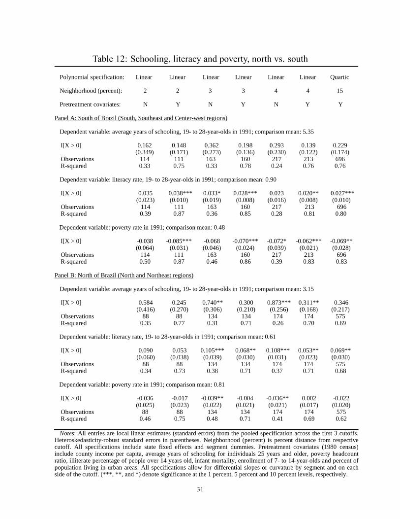
Table 12: Schooling, literacy and poverty, north vs. south
Polynomial specification: Linear Linear Linear Linear Linear Linear Quartic
Neighborhood (percent): 2 2 3 3 4 4 15
Pretreatment covariates: N Y N Y N Y Y
Panel A: South of Brazil (South, Southeast and Centerwest regions)
Dependent variable: average years of schooling, 19 to 28yearolds in 1991; comparison mean: 5.35
I[X > 0] 0.162 0.148 0.362 0.198 0.293 0.139 0.229(0.349) (0.171) (0.273) (0.136) (0.230) (0.122) (0.174)
Observations 114 111 163 160 217 213 696Rsquared 0.33 0.75 0.33 0.78 0.24 0.76 0.76
Dependent variable: literacy rate, 19 to 28yearolds in 1991; comparison mean: 0.90
I[X > 0] 0.035 0.038*** 0.033* 0.028*** 0.023 0.020** 0.027*** (0.023) (0.010) (0.019) (0.008) (0.016) (0.008) (0.010)
Observations 114 111 163 160 217 213 696Rsquared 0.39 0.87 0.36 0.85 0.28 0.81 0.80
Dependent variable: poverty rate in 1991; comparison mean: 0.48
I[X > 0] 0.038 0.085*** 0.068 0.070*** 0.072* 0.062*** 0.069** (0.064) (0.031) (0.046) (0.024) (0.039) (0.021) (0.028)
Observations 114 111 163 160 217 213 696Rsquared 0.50 0.87 0.46 0.86 0.39 0.83 0.83
Panel B: North of Brazil (North and Northeast regions)
Dependent variable: average years of schooling, 19 to 28yearolds in 1991; comparison mean: 3.15
I[X > 0] 0.584 0.245 0.740** 0.300 0.873*** 0.311** 0.346(0.416) (0.270) (0.306) (0.210) (0.256) (0.168) (0.217)
Observations 88 88 134 134 174 174 575Rsquared 0.35 0.77 0.31 0.71 0.26 0.70 0.69
Dependent variable: literacy rate, 19 to 28yearolds in 1991; comparison mean: 0.61
I[X > 0] 0.090 0.053 0.105*** 0.068** 0.108*** 0.053** 0.069**(0.060) (0.038) (0.039) (0.030) (0.031) (0.023) (0.030)
Observations 88 88 134 134 174 174 575Rsquared 0.34 0.73 0.38 0.71 0.37 0.71 0.68
Dependent variable: poverty rate in 1991; comparison mean: 0.81
I[X > 0] 0.036 0.017 0.039** 0.004 0.036** 0.002 0.022(0.025) (0.023) (0.022) (0.021) (0.021) (0.017) (0.020)
Observations 88 88 134 134 174 174 575Rsquared 0.46 0.75 0.48 0.71 0.41 0.69 0.62
Notes: All entries are local linear estimates (standard errors) from the pooled specification across the first 3 cutoffs.Heteroskedasticityrobust standard errors in parentheses. Neighborhood (percent) is percent distance from respectivecutoff. All specifications include state fixed effects and segment dummies. Pretreatment covariates (1980 census)include county income per capita, average years of schooling for individuals 25 years and older, poverty headcountratio, illiterate percentage of people over 14 years old, infant mortality, enrollment of 7 to 14yearolds and percent ofpopulation living in urban areas. All specifications allow for differential slopes or curvature by segment and on eachside of the cutoff. (***, **, and *) denote significance at the 1 percent, 5 percent and 10 percent levels, respectively.
31

Table 13: Total spending and teacher-student ration, urban vs. rural municipalities
Polynomial specification: Linear Linear Linear Linear Linear Linear Quartic
Neighborhood (percent): 2 2 3 3 4 4 15
Pretreatment covariates: N Y N Y N Y Y
Panel A: urban municipalities (percent urban residents in 1980 > 24.07)
Dependent variable: log total public spending per capita (19821985)
I[X > 0] 0.146 0.159 0.096 0.070 0.154* 0.136* 0.147**(0.134) (0.102) (0.103) (0.090) (0.089) (0.075) (0.061)
Observations 102 102 145 145 194 194 573Rsquared 0.72 0.84 0.69 0.78 0.59 0.72 0.75
Dependent variable: primary school teacherstudent ratio in 1991; comparison mean: 0.057
I[X > 0] 0.002 0.001 0.004 0.004 0.003 0.001 0.002(0.013) (0.012) (0.009) (0.008) (0.008) (0.007) (0.010)
Observations 78 78 117 117 155 155 508Rsquared 0.44 0.54 0.42 0.51 0.40 0.49 0.46
Panel B: rural municipalities (percent urban residents in 1980 < 24.07)
Dependent variable: log total public spending per capita (19821985)
I[X > 0] 0.168*** 0.268*** 0.221*** 0.225*** 0.215*** 0.196*** 0.178***(0.077) (0.072) (0.066) (0.064) (0.055) (0.052) (0.072)
Observations 93 93 143 143 186 186 612Rsquared 0.83 0.89 0.84 0.90 0.81 0.87 0.82
Dependent variable: primary school teacherstudent ratio in 1991; comparison mean: 0.050
I[X > 0] 0.012*** 0.011** 0.007** 0.007 0.008** 0.008*** 0.015***(0.004) (0.005) (0.004) (0.004) (0.003) (0.003) (0.004)
Observations 94 94 143 143 186 186 617Rsquared 0.62 0.63 0.60 0.63 0.56 0.59 0.57
Notes: All entries are local linear estimates (standard errors) from the pooled specification across the first 3 cutoffs.Heteroskedasticityrobust standard errors in parentheses. Neighborhood (percent) is percent distance from respectivecutoff. All specifications include state fixed effects and segment dummies. Pretreatment covariates (1980 census)include county income per capita, average years of schooling for individuals 25 years and older, poverty headcountratio, illiterate percentage of people over 14 years old, infant mortality, enrollment of 7 to 14yearolds and percent ofpopulation living in urban areas. All specifications allow for differential slopes or curvature by segment and on eachside of the cutoff. (***, **, and *) denote significance at the 1 percent, 5 percent and 10 percent levels, respectively.
32
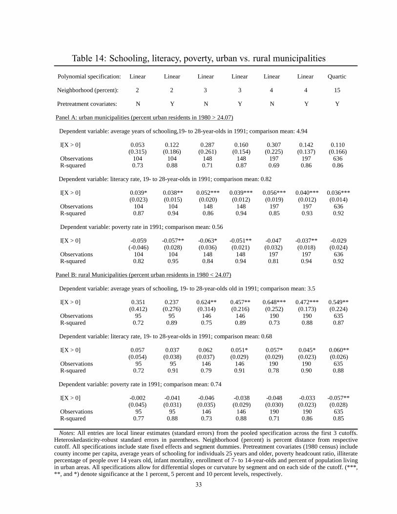
Table 14: Schooling, literacy, poverty, urban vs. rural municipalities
Polynomial specification: Linear Linear Linear Linear Linear Linear Quartic
Neighborhood (percent): 2 2 3 3 4 4 15
Pretreatment covariates: N Y N Y N Y Y
Panel A: urban municipalities (percent urban residents in 1980 > 24.07)
Dependent variable: average years of schooling,19 to 28yearolds in 1991; comparison mean: 4.94
I[X > 0] 0.053 0.122 0.287 0.160 0.307 0.142 0.110(0.315) (0.186) (0.261) (0.154) (0.225) (0.137) (0.166)
Observations 104 104 148 148 197 197 636Rsquared 0.73 0.88 0.71 0.87 0.69 0.86 0.86
Dependent variable: literacy rate, 19 to 28yearolds in 1991; comparison mean: 0.82
I[X > 0] 0.039* 0.038** 0.052*** 0.039*** 0.056*** 0.040*** 0.036***(0.023) (0.015) (0.020) (0.012) (0.019) (0.012) (0.014)
Observations 104 104 148 148 197 197 636Rsquared 0.87 0.94 0.86 0.94 0.85 0.93 0.92
Dependent variable: poverty rate in 1991; comparison mean: 0.56
I[X > 0] 0.059 0.057** 0.063* 0.051** 0.047 0.037** 0.029(0.046) (0.028) (0.036) (0.021) (0.032) (0.018) (0.024)
Observations 104 104 148 148 197 197 636Rsquared 0.82 0.95 0.84 0.94 0.81 0.94 0.92
Panel B: rural Municipalities (percent urban residents in 1980 < 24.07)
Dependent variable: average years of schooling, 19 to 28yearolds old in 1991; comparison mean: 3.5
I[X > 0] 0.351 0.237 0.624** 0.457** 0.648*** 0.472*** 0.549**(0.412) (0.276) (0.314) (0.216) (0.252) (0.173) (0.224)
Observations 95 95 146 146 190 190 635Rsquared 0.72 0.89 0.75 0.89 0.73 0.88 0.87
Dependent variable: literacy rate, 19 to 28yearolds in 1991; comparison mean: 0.68
I[X > 0] 0.057 0.037 0.062 0.051* 0.057* 0.045* 0.060**(0.054) (0.038) (0.037) (0.029) (0.029) (0.023) (0.026)
Observations 95 95 146 146 190 190 635 Rsquared 0.72 0.91 0.79 0.91 0.78 0.90 0.88
Dependent variable: poverty rate in 1991; comparison mean: 0.74
I[X > 0] 0.002 0.041 0.046 0.038 0.048 0.033 0.057**(0.045) (0.031) (0.035) (0.029) (0.030) (0.023) (0.028)
Observations 95 95 146 146 190 190 635Rsquared 0.77 0.88 0.73 0.88 0.71 0.86 0.85
Notes: All entries are local linear estimates (standard errors) from the pooled specification across the first 3 cutoffs.Heteroskedasticityrobust standard errors in parentheses. Neighborhood (percent) is percent distance from respectivecutoff. All specifications include state fixed effects and segment dummies. Pretreatment covariates (1980 census) includecounty income per capita, average years of schooling for individuals 25 years and older, poverty headcount ratio, illiteratepercentage of people over 14 years old, infant mortality, enrollment of 7 to 14yearolds and percent of population livingin urban areas. All specifications allow for differential slopes or curvature by segment and on each side of the cutoff. (***,**, and *) denote significance at the 1 percent, 5 percent and 10 percent levels, respectively.
33