online edition (c)2009 cambridge up - the stanford … · online edition (c) 2009 cambridge up 378...


DRAFT! © April 1, 2009 Cambridge University Press. Feedback welcome. 377

17 Hierarchical clustering

Flat clustering is efficient and conceptually simple, but as we saw in Chap-ter 16 it has a number of drawbacks. The algorithms introduced in Chap-ter 16 return a flat unstructured set of clusters, require a prespecified num-ber of clusters as input and are nondeterministic. Hierarchical clustering (orHIERARCHICAL

CLUSTERING hierarchic clustering) outputs a hierarchy, a structure that is more informativethan the unstructured set of clusters returned by flat clustering.1 Hierarchicalclustering does not require us to prespecify the number of clusters and mosthierarchical algorithms that have been used in IR are deterministic. These ad-vantages of hierarchical clustering come at the cost of lower efficiency. Themost common hierarchical clustering algorithms have a complexity that is atleast quadratic in the number of documents compared to the linear complex-ity of K-means and EM (cf. Section 16.4, page 364).

This chapter first introduces agglomerative hierarchical clustering (Section 17.1)and presents four different agglomerative algorithms, in Sections 17.2–17.4,which differ in the similarity measures they employ: single-link, complete-link, group-average, and centroid similarity. We then discuss the optimalityconditions of hierarchical clustering in Section 17.5. Section 17.6 introducestop-down (or divisive) hierarchical clustering. Section 17.7 looks at labelingclusters automatically, a problem that must be solved whenever humans in-teract with the output of clustering. We discuss implementation issues inSection 17.8. Section 17.9 provides pointers to further reading, including ref-erences to soft hierarchical clustering, which we do not cover in this book.

There are few differences between the applications of flat and hierarchi-cal clustering in information retrieval. In particular, hierarchical clusteringis appropriate for any of the applications shown in Table 16.1 (page 351; seealso Section 16.6, page 372). In fact, the example we gave for collection clus-tering is hierarchical. In general, we select flat clustering when efficiencyis important and hierarchical clustering when one of the potential problems

1. In this chapter, we only consider hierarchies that are binary trees like the one shown in Fig-ure 17.1 – but hierarchical clustering can be easily extended to other types of trees.


378 17 Hierarchical clustering

of flat clustering (not enough structure, predetermined number of clusters,non-determinism) is a concern. In addition, many researchers believe that hi-erarchical clustering produces better clusters than flat clustering. However,there is no consensus on this issue (see references in Section 17.9).

17.1 Hierarchical agglomerative clustering

Hierarchical clustering algorithms are either top-down or bottom-up. Bottom-up algorithms treat each document as a singleton cluster at the outset andthen successively merge (or agglomerate) pairs of clusters until all clustershave been merged into a single cluster that contains all documents. Bottom-up hierarchical clustering is therefore called hierarchical agglomerative cluster-HIERARCHICAL

AGGLOMERATIVE

CLUSTERINGing or HAC. Top-down clustering requires a method for splitting a cluster.

HACIt proceeds by splitting clusters recursively until individual documents arereached. See Section 17.6. HAC is more frequently used in IR than top-downclustering and is the main subject of this chapter.

Before looking at specific similarity measures used in HAC in Sections17.2–17.4, we first introduce a method for depicting hierarchical clusteringsgraphically, discuss a few key properties of HACs and present a simple algo-rithm for computing an HAC.

An HAC clustering is typically visualized as a dendrogram as shown inDENDROGRAM

Figure 17.1. Each merge is represented by a horizontal line. The y-coordinateof the horizontal line is the similarity of the two clusters that were merged,where documents are viewed as singleton clusters. We call this similarity thecombination similarity of the merged cluster. For example, the combinationCOMBINATION

SIMILARITY similarity of the cluster consisting of Lloyd’s CEO questioned and Lloyd’s chief/ U.S. grilling in Figure 17.1 is ≈ 0.56. We define the combination similarityof a singleton cluster as its document’s self-similarity (which is 1.0 for cosinesimilarity).

By moving up from the bottom layer to the top node, a dendrogram al-lows us to reconstruct the history of merges that resulted in the depictedclustering. For example, we see that the two documents entitled War heroColin Powell were merged first in Figure 17.1 and that the last merge addedAg trade reform to a cluster consisting of the other 29 documents.

A fundamental assumption in HAC is that the merge operation is mono-MONOTONICITY

tonic. Monotonic means that if s1, s2, . . . , sK−1 are the combination similaritiesof the successive merges of an HAC, then s1 ≥ s2 ≥ . . . ≥ sK−1 holds. A non-monotonic hierarchical clustering contains at least one inversion si < si+1INVERSION

and contradicts the fundamental assumption that we chose the best mergeavailable at each step. We will see an example of an inversion in Figure 17.12.

Hierarchical clustering does not require a prespecified number of clusters.However, in some applications we want a partition of disjoint clusters just as

On

line ed

ition

(c)2009 Cam

brid

ge U

P

17.1H

ierarchicalagglom

erativeclu

stering

37

9

1.0 0.8 0.6 0.4 0.2 0.0

Ag trade reform.Back−to−school spending is up

Lloyd’s CEO questionedLloyd’s chief / U.S. grilling

Viag stays positiveChrysler / Latin America

Ohio Blue CrossJapanese prime minister / Mexico

CompuServe reports lossSprint / Internet access service

Planet HollywoodTrocadero: tripling of revenues

German unions splitWar hero Colin PowellWar hero Colin Powell

Oil prices slipChains may raise prices

Clinton signs lawLawsuit against tobacco companies

suits against tobacco firmsIndiana tobacco lawsuit

Most active stocksMexican markets

Hog prices tumbleNYSE closing averages

British FTSE indexFed holds interest rates steady

Fed to keep interest rates steadyFed keeps interest rates steadyFed keeps interest rates steady

F

igu

re17.1

Ad

end

rog

ramo

fa

sing

le-link

clusterin

go

f30

do

cum

ents

from

Reu

ters-RC

V1.

Tw

op

ossib

lecu

tso

fth

ed

end

rog

ramare

sho

wn

:at

0.4in

to24

clusters

and

at0.1

into

12clu

sters.



in flat clustering. In those cases, the hierarchy needs to be cut at some point.A number of criteria can be used to determine the cutting point:

• Cut at a prespecified level of similarity. For example, we cut the dendro-gram at 0.4 if we want clusters with a minimum combination similarityof 0.4. In Figure 17.1, cutting the diagram at y = 0.4 yields 24 clusters(grouping only documents with high similarity together) and cutting it aty = 0.1 yields 12 clusters (one large financial news cluster and 11 smallerclusters).

• Cut the dendrogram where the gap between two successive combinationsimilarities is largest. Such large gaps arguably indicate “natural” clus-terings. Adding one more cluster decreases the quality of the clusteringsignificantly, so cutting before this steep decrease occurs is desirable. Thisstrategy is analogous to looking for the knee in the K-means graph in Fig-ure 16.8 (page 366).

• Apply Equation (16.11) (page 366):

K = arg minK′

[RSS(K′) + λK′]

where K′ refers to the cut of the hierarchy that results in K′ clusters, RSS isthe residual sum of squares and λ is a penalty for each additional cluster.Instead of RSS, another measure of distortion can be used.

• As in flat clustering, we can also prespecify the number of clusters K andselect the cutting point that produces K clusters.

A simple, naive HAC algorithm is shown in Figure 17.2. We first computethe N × N similarity matrix C. The algorithm then executes N − 1 stepsof merging the currently most similar clusters. In each iteration, the twomost similar clusters are merged and the rows and columns of the mergedcluster i in C are updated.2 The clustering is stored as a list of merges inA. I indicates which clusters are still available to be merged. The functionSIM(i, m, j) computes the similarity of cluster j with the merge of clusters iand m. For some HAC algorithms, SIM(i, m, j) is simply a function of C[j][i]and C[j][m], for example, the maximum of these two values for single-link.

We will now refine this algorithm for the different similarity measuresof single-link and complete-link clustering (Section 17.2) and group-averageand centroid clustering (Sections 17.3 and 17.4). The merge criteria of thesefour variants of HAC are shown in Figure 17.3.

2. We assume that we use a deterministic method for breaking ties, such as always choose themerge that is the first cluster with respect to a total ordering of the subsets of the document setD.


17.1 Hierarchical agglomerative clustering 381

SIMPLEHAC(d1, . . . , dN)1 for n← 1 to N2 do for i← 1 to N3 do C[n][i]← SIM(dn, di)4 I[n]← 1 (keeps track of active clusters)5 A← [] (assembles clustering as a sequence of merges)6 for k← 1 to N − 17 do 〈i, m〉 ← arg max〈i,m〉:i 6=m∧I[i]=1∧I[m]=1C[i][m]

8 A.APPEND(〈i, m〉) (store merge)9 for j← 1 to N

10 do C[i][j]← SIM(i, m, j)11 C[j][i]← SIM(i, m, j)12 I[m]← 0 (deactivate cluster)13 return A

Figure 17.2 A simple, but inefficient HAC algorithm.

b

b

b

b

(a) single-link: maximum similarity

b

b

b

b

(b) complete-link: minimum similarity

b

b

b

b

(c) centroid: average inter-similarity

b

b

b

b

(d) group-average: average of all similarities

Figure 17.3 The different notions of cluster similarity used by the four HAC al-gorithms. An inter-similarity is a similarity between two documents from differentclusters.



0 1 2 3 40

1

2

3

×

d5

×

d6

×

d7

×

d8

×

d1

×

d2

×

d3

×

d4

0 1 2 3 40

1

2

3

×

d5

×

d6

×

d7

×

d8

×

d1

×

d2

×

d3

×

d4

Figure 17.4 A single-link (left) and complete-link (right) clustering of eight doc-uments. The ellipses correspond to successive clustering stages. Left: The single-linksimilarity of the two upper two-point clusters is the similarity of d2 and d3 (solidline), which is greater than the single-link similarity of the two left two-point clusters(dashed line). Right: The complete-link similarity of the two upper two-point clustersis the similarity of d1 and d4 (dashed line), which is smaller than the complete-linksimilarity of the two left two-point clusters (solid line).

17.2 Single-link and complete-link clustering

In single-link clustering or single-linkage clustering, the similarity of two clus-SINGLE-LINK

CLUSTERING ters is the similarity of their most similar members (see Figure 17.3, (a))3. Thissingle-link merge criterion is local. We pay attention solely to the area wherethe two clusters come closest to each other. Other, more distant parts of thecluster and the clusters’ overall structure are not taken into account.

In complete-link clustering or complete-linkage clustering, the similarity of twoCOMPLETE-LINK

CLUSTERING clusters is the similarity of their most dissimilar members (see Figure 17.3, (b)).This is equivalent to choosing the cluster pair whose merge has the smallestdiameter. This complete-link merge criterion is non-local; the entire structureof the clustering can influence merge decisions. This results in a preferencefor compact clusters with small diameters over long, straggly clusters, butalso causes sensitivity to outliers. A single document far from the center canincrease diameters of candidate merge clusters dramatically and completelychange the final clustering.

Figure 17.4 depicts a single-link and a complete-link clustering of eightdocuments. The first four steps, each producing a cluster consisting of a pairof two documents, are identical. Then single-link clustering joins the up-per two pairs (and after that the lower two pairs) because on the maximum-similarity definition of cluster similarity, those two clusters are closest. Complete-

3. Throughout this chapter, we equate similarity with proximity in 2D depictions of clustering.

On

line ed

ition

(c)2009 Cam

brid

ge U

P

17.2S

ingle-lin

kan

dcom

plete-link

clusterin

g3

83

1.0 0.8 0.6 0.4 0.2 0.0

NYSE closing averagesHog prices tumble

Oil prices slipAg trade reform.

Chrysler / Latin AmericaJapanese prime minister / Mexico

Fed holds interest rates steadyFed to keep interest rates steady

Fed keeps interest rates steadyFed keeps interest rates steady

Mexican marketsBritish FTSE index

War hero Colin PowellWar hero Colin Powell

Lloyd’s CEO questionedLloyd’s chief / U.S. grilling

Ohio Blue CrossLawsuit against tobacco companies

suits against tobacco firmsIndiana tobacco lawsuit

Viag stays positiveMost active stocks

CompuServe reports lossSprint / Internet access service

Planet HollywoodTrocadero: tripling of revenues

Back−to−school spending is upGerman unions split

Chains may raise pricesClinton signs law

F

igu

re17.5

Ad

end

rog

ramo

fa

com

plete-lin

kclu

stering

.T

he

same

30d

ocu

men

tsw

ereclu

steredw

ithsin

gle-lin

kclu

stering

inF

igu

re17.1.



× × × × × ×

× × × × × ×

Figure 17.6 Chaining in single-link clustering. The local criterion in single-linkclustering can cause undesirable elongated clusters.

link clustering joins the left two pairs (and then the right two pairs) becausethose are the closest pairs according to the minimum-similarity definition ofcluster similarity.4

Figure 17.1 is an example of a single-link clustering of a set of documentsand Figure 17.5 is the complete-link clustering of the same set. When cuttingthe last merge in Figure 17.5, we obtain two clusters of similar size (doc-uments 1–16, from NYSE closing averages to Lloyd’s chief / U.S. grilling, anddocuments 17–30, from Ohio Blue Cross to Clinton signs law). There is no cutof the dendrogram in Figure 17.1 that would give us an equally balancedclustering.

Both single-link and complete-link clustering have graph-theoretic inter-pretations. Define sk to be the combination similarity of the two clustersmerged in step k, and G(sk) the graph that links all data points with a similar-ity of at least sk. Then the clusters after step k in single-link clustering are theconnected components of G(sk) and the clusters after step k in complete-linkclustering are maximal cliques of G(sk). A connected component is a maximalCONNECTED

COMPONENT set of connected points such that there is a path connecting each pair. A cliqueCLIQUE is a set of points that are completely linked with each other.

These graph-theoretic interpretations motivate the terms single-link andcomplete-link clustering. Single-link clusters at step k are maximal sets ofpoints that are linked via at least one link (a single link) of similarity s ≥ sk;complete-link clusters at step k are maximal sets of points that are completelylinked with each other via links of similarity s ≥ sk.

Single-link and complete-link clustering reduce the assessment of clusterquality to a single similarity between a pair of documents: the two most sim-ilar documents in single-link clustering and the two most dissimilar docu-ments in complete-link clustering. A measurement based on one pair cannotfully reflect the distribution of documents in a cluster. It is therefore not sur-prising that both algorithms often produce undesirable clusters. Single-linkclustering can produce straggling clusters as shown in Figure 17.6. Since themerge criterion is strictly local, a chain of points can be extended for long

4. If you are bothered by the possibility of ties, assume that d1 has coordinates (1 + ǫ, 3− ǫ) andthat all other points have integer coordinates.


17.2 Single-link and complete-link clustering 385

0 1 2 3 4 5 6 70

1 ×

d1

×

d2

×

d3

×

d4

×

d5

Figure 17.7 Outliers in complete-link clustering. The five documents havethe x-coordinates 1 + 2ǫ, 4, 5 + 2ǫ, 6 and 7 − ǫ. Complete-link clustering cre-ates the two clusters shown as ellipses. The most intuitive two-cluster cluster-ing is d1, d2, d3, d4, d5, but in complete-link clustering, the outlier d1 splitsd2, d3, d4, d5 as shown.

distances without regard to the overall shape of the emerging cluster. Thiseffect is called chaining.CHAINING

The chaining effect is also apparent in Figure 17.1. The last eleven mergesof the single-link clustering (those above the 0.1 line) add on single docu-ments or pairs of documents, corresponding to a chain. The complete-linkclustering in Figure 17.5 avoids this problem. Documents are split into twogroups of roughly equal size when we cut the dendrogram at the last merge.In general, this is a more useful organization of the data than a clusteringwith chains.

However, complete-link clustering suffers from a different problem. Itpays too much attention to outliers, points that do not fit well into the globalstructure of the cluster. In the example in Figure 17.7 the four documentsd2, d3, d4, d5 are split because of the outlier d1 at the left edge (Exercise 17.1).Complete-link clustering does not find the most intuitive cluster structure inthis example.

17.2.1 Time complexity of HAC

The complexity of the naive HAC algorithm in Figure 17.2 is Θ(N3) becausewe exhaustively scan the N × N matrix C for the largest similarity in each ofN − 1 iterations.

For the four HAC methods discussed in this chapter a more efficient algo-rithm is the priority-queue algorithm shown in Figure 17.8. Its time complex-ity is Θ(N2 log N). The rows C[k] of the N× N similarity matrix C are sortedin decreasing order of similarity in the priority queues P. P[k].MAX() thenreturns the cluster in P[k] that currently has the highest similarity with ωk,where we use ωk to denote the kth cluster as in Chapter 16. After creating themerged cluster of ωk1

and ωk2, ωk1

is used as its representative. The functionSIM computes the similarity function for potential merge pairs: largest simi-larity for single-link, smallest similarity for complete-link, average similarityfor GAAC (Section 17.3), and centroid similarity for centroid clustering (Sec-



EFFICIENTHAC(~d1, . . . , ~dN)1 for n← 1 to N2 do for i ← 1 to N3 do C[n][i].sim← ~dn · ~di

4 C[n][i].index← i5 I[n]← 16 P[n]← priority queue for C[n] sorted on sim7 P[n].DELETE(C[n][n]) (don’t want self-similarities)8 A ← []9 for k← 1 to N − 1

10 do k1 ← arg maxk:I[k]=1 P[k].MAX().sim

11 k2 ← P[k1].MAX().index12 A.APPEND(〈k1, k2〉)13 I[k2]← 014 P[k1]← []15 for each i with I[i] = 1 ∧ i 6= k1

16 do P[i].DELETE(C[i][k1])17 P[i].DELETE(C[i][k2])18 C[i][k1].sim← SIM(i, k1, k2)19 P[i].INSERT(C[i][k1])20 C[k1][i].sim← SIM(i, k1, k2)21 P[k1].INSERT(C[k1][i])22 return A

clustering algorithm SIM(i, k1, k2)single-link max(SIM(i, k1), SIM(i, k2))complete-link min(SIM(i, k1), SIM(i, k2))centroid ( 1

Nm~vm) · ( 1

Ni~vi)

group-average 1(Nm+Ni)(Nm+Ni−1)

[(~vm +~vi)2 − (Nm + Ni)]

compute C[5]1 2 3 4 50.2 0.8 0.6 0.4 1.0

create P[5] (by sorting)2 3 4 10.8 0.6 0.4 0.2

merge 2 and 3, updatesimilarity of 2, delete 3

2 4 10.3 0.4 0.2

delete and reinsert 24 2 10.4 0.3 0.2

Figure 17.8 The priority-queue algorithm for HAC. Top: The algorithm. Center:Four different similarity measures. Bottom: An example for processing steps 6 and16–19. This is a made up example showing P[5] for a 5× 5 matrix C.


17.2 Single-link and complete-link clustering 387

SINGLELINKCLUSTERING(d1, . . . , dN)1 for n← 1 to N2 do for i← 1 to N3 do C[n][i].sim← SIM(dn, di)4 C[n][i].index← i5 I[n]← n6 NBM[n]← arg maxX∈C[n][i]:n 6=iX.sim

7 A← []8 for n← 1 to N − 19 do i1 ← arg maxi:I[i]=iNBM[i].sim

10 i2 ← I[NBM[i1].index]11 A.APPEND(〈i1, i2〉)12 for i← 1 to N13 do if I[i] = i ∧ i 6= i1 ∧ i 6= i214 then C[i1][i].sim← C[i][i1].sim← max(C[i1][i].sim, C[i2][i].sim)15 if I[i] = i216 then I[i]← i117 NBM[i1]← arg maxX∈C[i1][i]:I[i]=i∧i 6=i1 X.sim

18 return A

Figure 17.9 Single-link clustering algorithm using an NBM array. After mergingtwo clusters i1 and i2, the first one (i1) represents the merged cluster. If I[i] = i, then iis the representative of its current cluster. If I[i] 6= i, then i has been merged into thecluster represented by I[i] and will therefore be ignored when updating NBM[i1].

tion 17.4). We give an example of how a row of C is processed (Figure 17.8,bottom panel). The loop in lines 1–7 is Θ(N2) and the loop in lines 9–21 isΘ(N2 log N) for an implementation of priority queues that supports deletionand insertion in Θ(log N). The overall complexity of the algorithm is there-fore Θ(N2 log N). In the definition of the function SIM, ~vm and ~vi are thevector sums of ωk1

∪ωk2and ωi, respectively, and Nm and Ni are the number

of documents in ωk1∪ωk2

and ωi, respectively.The argument of EFFICIENTHAC in Figure 17.8 is a set of vectors (as op-

posed to a set of generic documents) because GAAC and centroid clustering(Sections 17.3 and 17.4) require vectors as input. The complete-link versionof EFFICIENTHAC can also be applied to documents that are not representedas vectors.

For single-link, we can introduce a next-best-merge array (NBM) as a fur-ther optimization as shown in Figure 17.9. NBM keeps track of what the bestmerge is for each cluster. Each of the two top level for-loops in Figure 17.9are Θ(N2), thus the overall complexity of single-link clustering is Θ(N2).



0 1 2 3 4 5 6 7 8 9 100

1 ×

d1

×

d2

×

d3

×

d4

Figure 17.10 Complete-link clustering is not best-merge persistent. At first, d2 isthe best-merge cluster for d3. But after merging d1 and d2, d4 becomes d3’s best-mergecandidate. In a best-merge persistent algorithm like single-link, d3’s best-merge clus-ter would be d1, d2.

Can we also speed up the other three HAC algorithms with an NBM ar-ray? We cannot because only single-link clustering is best-merge persistent.BEST-MERGE

PERSISTENCE Suppose that the best merge cluster for ωk is ωj in single-link clustering.Then after merging ωj with a third cluster ωi 6= ωk, the merge of ωi and ωj

will be ωk’s best merge cluster (Exercise 17.6). In other words, the best-mergecandidate for the merged cluster is one of the two best-merge candidates ofits components in single-link clustering. This means that C can be updatedin Θ(N) in each iteration – by taking a simple max of two values on line 14in Figure 17.9 for each of the remaining ≤ N clusters.

Figure 17.10 demonstrates that best-merge persistence does not hold forcomplete-link clustering, which means that we cannot use an NBM array tospeed up clustering. After merging d3’s best merge candidate d2 with clusterd1, an unrelated cluster d4 becomes the best merge candidate for d3. This isbecause the complete-link merge criterion is non-local and can be affected bypoints at a great distance from the area where two merge candidates meet.

In practice, the efficiency penalty of the Θ(N2 log N) algorithm is smallcompared with the Θ(N2) single-link algorithm since computing the similar-ity between two documents (e.g., as a dot product) is an order of magnitudeslower than comparing two scalars in sorting. All four HAC algorithms inthis chapter are Θ(N2) with respect to similarity computations. So the differ-ence in complexity is rarely a concern in practice when choosing one of thealgorithms.

? Exercise 17.1

Show that complete-link clustering creates the two-cluster clustering depicted in Fig-ure 17.7.

17.3 Group-average agglomerative clustering

Group-average agglomerative clustering or GAAC (see Figure 17.3, (d)) evaluatesGROUP-AVERAGE

AGGLOMERATIVE

CLUSTERINGcluster quality based on all similarities between documents, thus avoidingthe pitfalls of the single-link and complete-link criteria, which equate cluster


17.3 Group-average agglomerative clustering 389

similarity with the similarity of a single pair of documents. GAAC is alsocalled group-average clustering and average-link clustering. GAAC computesthe average similarity SIM-GA of all pairs of documents, including pairs fromthe same cluster. But self-similarities are not included in the average:

SIM-GA(ωi, ωj) =1

(Ni + Nj)(Ni + Nj − 1) ∑dm∈ωi∪ωj

∑dn∈ωi∪ωj,dn 6=dm

~dm · ~dn(17.1)

where ~d is the length-normalized vector of document d, · denotes the dotproduct, and Ni and Nj are the number of documents in ωi and ωj, respec-tively.

The motivation for GAAC is that our goal in selecting two clusters ωi

and ωj as the next merge in HAC is that the resulting merge cluster ωk =ωi ∪ ωj should be coherent. To judge the coherence of ωk, we need to lookat all document-document similarities within ωk, including those that occurwithin ωi and those that occur within ωj.

We can compute the measure SIM-GA efficiently because the sum of indi-vidual vector similarities is equal to the similarities of their sums:

∑dm∈ωi

∑dn∈ωj

(~dm · ~dn) = ( ∑dm∈ωi

~dm) · ( ∑dn∈ωj

~dn)(17.2)

With (17.2), we have:

SIM-GA(ωi, ωj) =1

(Ni + Nj)(Ni + Nj − 1)[( ∑

dm∈ωi∪ωj

~dm)2 − (Ni + Nj)](17.3)

The term (Ni + Nj) on the right is the sum of Ni + Nj self-similarities of value1.0. With this trick we can compute cluster similarity in constant time (as-

suming we have available the two vector sums ∑dm∈ωi~dm and ∑dm∈ωj

~dm)

instead of in Θ(NiNj). This is important because we need to be able to com-pute the function SIM on lines 18 and 20 in EFFICIENTHAC (Figure 17.8)in constant time for efficient implementations of GAAC. Note that for twosingleton clusters, Equation (17.3) is equivalent to the dot product.

Equation (17.2) relies on the distributivity of the dot product with respectto vector addition. Since this is crucial for the efficient computation of aGAAC clustering, the method cannot be easily applied to representations ofdocuments that are not real-valued vectors. Also, Equation (17.2) only holdsfor the dot product. While many algorithms introduced in this book havenear-equivalent descriptions in terms of dot product, cosine similarity andEuclidean distance (cf. Section 14.1, page 291), Equation (17.2) can only beexpressed using the dot product. This is a fundamental difference betweensingle-link/complete-link clustering and GAAC. The first two only require a



square matrix of similarities as input and do not care how these similaritieswere computed.

To summarize, GAAC requires (i) documents represented as vectors, (ii)length normalization of vectors, so that self-similarities are 1.0, and (iii) thedot product as the measure of similarity between vectors and sums of vec-tors.

The merge algorithms for GAAC and complete-link clustering are the sameexcept that we use Equation (17.3) as similarity function in Figure 17.8. There-fore, the overall time complexity of GAAC is the same as for complete-linkclustering: Θ(N2 log N). Like complete-link clustering, GAAC is not best-merge persistent (Exercise 17.6). This means that there is no Θ(N2) algorithmfor GAAC that would be analogous to the Θ(N2) algorithm for single-link inFigure 17.9.

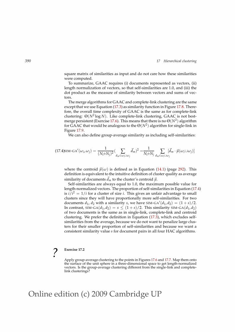
We can also define group-average similarity as including self-similarities:

SIM-GA′(ωi, ωj) =

1

(Ni+Nj)2( ∑

dm∈ωi∪ωj

~dm)2 =1

Ni+Nj∑

dm∈ωi∪ωj

[~dm ·~µ(ωi∪ωj)](17.4)

where the centroid ~µ(ω) is defined as in Equation (14.1) (page 292). Thisdefinition is equivalent to the intuitive definition of cluster quality as average

similarity of documents ~dm to the cluster’s centroid ~µ.Self-similarities are always equal to 1.0, the maximum possible value for

length-normalized vectors. The proportion of self-similarities in Equation (17.4)is i/i2 = 1/i for a cluster of size i. This gives an unfair advantage to smallclusters since they will have proportionally more self-similarities. For twodocuments d1, d2 with a similarity s, we have SIM-GA′(d1, d2) = (1 + s)/2.In contrast, SIM-GA(d1, d2) = s ≤ (1 + s)/2. This similarity SIM-GA(d1, d2)of two documents is the same as in single-link, complete-link and centroidclustering. We prefer the definition in Equation (17.3), which excludes self-similarities from the average, because we do not want to penalize large clus-ters for their smaller proportion of self-similarities and because we want aconsistent similarity value s for document pairs in all four HAC algorithms.

? Exercise 17.2

Apply group-average clustering to the points in Figures 17.6 and 17.7. Map them ontothe surface of the unit sphere in a three-dimensional space to get length-normalizedvectors. Is the group-average clustering different from the single-link and complete-link clusterings?


17.4 Centroid clustering 391

0 1 2 3 4 5 6 70

1

2

3

4

5 × d1

× d2

× d3

× d4

×d5 × d6bc

µ1

bcµ3

bc µ2

Figure 17.11 Three iterations of centroid clustering. Each iteration merges thetwo clusters whose centroids are closest.

17.4 Centroid clustering

In centroid clustering, the similarity of two clusters is defined as the similar-ity of their centroids:

SIM-CENT(ωi, ωj) = ~µ(ωi) ·~µ(ωj)(17.5)

= (1

Ni∑

dm∈ωi

~dm) · ( 1

Nj∑

dn∈ωj

~dn)

=1

NiNj∑

dm∈ωi

∑dn∈ωj

~dm · ~dn(17.6)

Equation (17.5) is centroid similarity. Equation (17.6) shows that centroidsimilarity is equivalent to average similarity of all pairs of documents fromdifferent clusters. Thus, the difference between GAAC and centroid clusteringis that GAAC considers all pairs of documents in computing average pair-wise similarity (Figure 17.3, (d)) whereas centroid clustering excludes pairsfrom the same cluster (Figure 17.3, (c)).

Figure 17.11 shows the first three steps of a centroid clustering. The firsttwo iterations form the clusters d5, d6 with centroid µ1 and d1, d2 withcentroid µ2 because the pairs 〈d5, d6〉 and 〈d1, d2〉 have the highest centroidsimilarities. In the third iteration, the highest centroid similarity is betweenµ1 and d4 producing the cluster d4, d5, d6 with centroid µ3.

Like GAAC, centroid clustering is not best-merge persistent and thereforeΘ(N2 log N) (Exercise 17.6).

In contrast to the other three HAC algorithms, centroid clustering is notmonotonic. So-called inversions can occur: Similarity can increase duringINVERSION



0 1 2 3 4 50

1

2

3

4

5

× ×

×

bc

d1 d2

d3

−4

−3

−2

−1

0d1 d2 d3

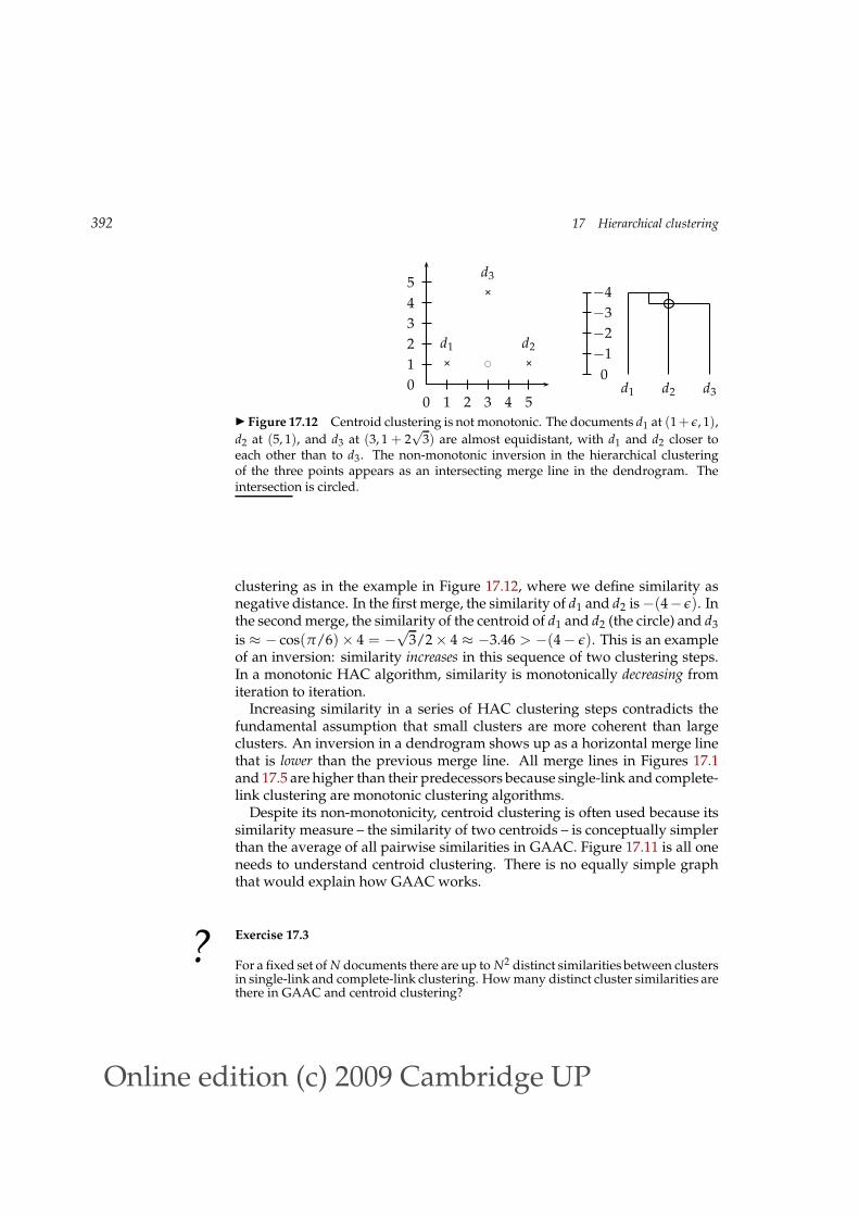
Figure 17.12 Centroid clustering is not monotonic. The documents d1 at (1 + ǫ, 1),

d2 at (5, 1), and d3 at (3, 1 + 2√

3) are almost equidistant, with d1 and d2 closer toeach other than to d3. The non-monotonic inversion in the hierarchical clusteringof the three points appears as an intersecting merge line in the dendrogram. Theintersection is circled.

clustering as in the example in Figure 17.12, where we define similarity asnegative distance. In the first merge, the similarity of d1 and d2 is−(4− ǫ). Inthe second merge, the similarity of the centroid of d1 and d2 (the circle) and d3

is ≈ − cos(π/6)× 4 = −√

3/2× 4 ≈ −3.46 > −(4− ǫ). This is an exampleof an inversion: similarity increases in this sequence of two clustering steps.In a monotonic HAC algorithm, similarity is monotonically decreasing fromiteration to iteration.

Increasing similarity in a series of HAC clustering steps contradicts thefundamental assumption that small clusters are more coherent than largeclusters. An inversion in a dendrogram shows up as a horizontal merge linethat is lower than the previous merge line. All merge lines in Figures 17.1and 17.5 are higher than their predecessors because single-link and complete-link clustering are monotonic clustering algorithms.

Despite its non-monotonicity, centroid clustering is often used because itssimilarity measure – the similarity of two centroids – is conceptually simplerthan the average of all pairwise similarities in GAAC. Figure 17.11 is all oneneeds to understand centroid clustering. There is no equally simple graphthat would explain how GAAC works.

? Exercise 17.3

For a fixed set of N documents there are up to N2 distinct similarities between clustersin single-link and complete-link clustering. How many distinct cluster similarities arethere in GAAC and centroid clustering?


17.5 Optimality of HAC 393

17.5 Optimality of HAC

To state the optimality conditions of hierarchical clustering precisely, we firstdefine the combination similarity COMB-SIM of a clustering Ω = ω1, . . . , ωKas the smallest combination similarity of any of its K clusters:

COMB-SIM(ω1, . . . , ωK) = mink

COMB-SIM(ωk)

Recall that the combination similarity of a cluster ω that was created as themerge of ω1 and ω2 is the similarity of ω1 and ω2 (page 378).

We then define Ω = ω1, . . . , ωK to be optimal if all clusterings Ω′ with kOPTIMAL CLUSTERING

clusters, k ≤ K, have lower combination similarities:

|Ω′| ≤ |Ω| ⇒ COMB-SIM(Ω′) ≤ COMB-SIM(Ω)

Figure 17.12 shows that centroid clustering is not optimal. The cluster-ing d1, d2, d3 (for K = 2) has combination similarity −(4 − ǫ) andd1, d2, d3 (for K = 1) has combination similarity -3.46. So the cluster-ing d1, d2, d3 produced in the first merge is not optimal since there isa clustering with fewer clusters (d1, d2, d3) that has higher combinationsimilarity. Centroid clustering is not optimal because inversions can occur.

The above definition of optimality would be of limited use if it was onlyapplicable to a clustering together with its merge history. However, we canshow (Exercise 17.4) that combination similarity for the three non-inversionCOMBINATION

SIMILARITY algorithms can be read off from the cluster without knowing its history. Thesedirect definitions of combination similarity are as follows.

single-link The combination similarity of a cluster ω is the smallest similar-ity of any bipartition of the cluster, where the similarity of a bipartition isthe largest similarity between any two documents from the two parts:

COMB-SIM(ω) = minω′:ω′⊂ω

maxdi∈ω′

maxd j∈ω−ω′

SIM(di, dj)

where each 〈ω′, ω− ω′〉 is a bipartition of ω.

complete-link The combination similarity of a cluster ω is the smallest sim-ilarity of any two points in ω: mindi∈ω mind j∈ω SIM(di, dj).

GAAC The combination similarity of a cluster ω is the average of all pair-wise similarities in ω (where self-similarities are not included in the aver-age): Equation (17.3).

If we use these definitions of combination similarity, then optimality is aproperty of a set of clusters and not of a process that produces a set of clus-ters.



We can now prove the optimality of single-link clustering by inductionover the number of clusters K. We will give a proof for the case where no twopairs of documents have the same similarity, but it can easily be extended tothe case with ties.

The inductive basis of the proof is that a clustering with K = N clusters hascombination similarity 1.0, which is the largest value possible. The induc-tion hypothesis is that a single-link clustering ΩK with K clusters is optimal:COMB-SIM(ΩK) ≥ COMB-SIM(Ω′K) for all Ω′K. Assume for contradiction thatthe clustering ΩK−1 we obtain by merging the two most similar clusters inΩK is not optimal and that instead a different sequence of merges Ω′K, Ω′K−1leads to the optimal clustering with K − 1 clusters. We can write the as-sumption that Ω′K−1 is optimal and that ΩK−1 is not as COMB-SIM(Ω′K−1) >

COMB-SIM(ΩK−1).Case 1: The two documents linked by s = COMB-SIM(Ω′K−1) are in the

same cluster in ΩK. They can only be in the same cluster if a merge with sim-ilarity smaller than s has occurred in the merge sequence producing ΩK. Thisimplies s > COMB-SIM(ΩK). Thus, COMB-SIM(Ω′K−1) = s > COMB-SIM(ΩK) >

COMB-SIM(Ω′K) > COMB-SIM(Ω′K−1). Contradiction.Case 2: The two documents linked by s = COMB-SIM(Ω′K−1) are not in

the same cluster in ΩK. But s = COMB-SIM(Ω′K−1) > COMB-SIM(ΩK−1), sothe single-link merging rule should have merged these two clusters whenprocessing ΩK. Contradiction.

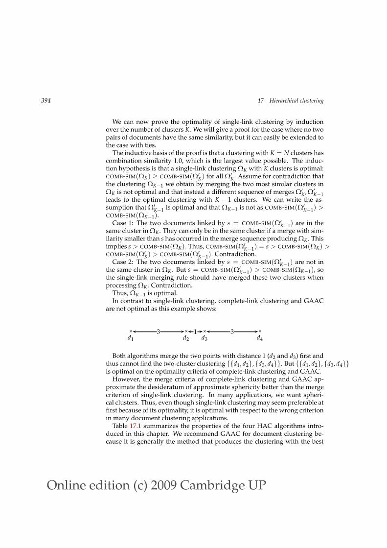
Thus, ΩK−1 is optimal.In contrast to single-link clustering, complete-link clustering and GAAC

are not optimal as this example shows:

× × × ×13 3d1 d2 d3 d4

Both algorithms merge the two points with distance 1 (d2 and d3) first andthus cannot find the two-cluster clustering d1, d2, d3, d4. But d1, d2, d3, d4is optimal on the optimality criteria of complete-link clustering and GAAC.

However, the merge criteria of complete-link clustering and GAAC ap-proximate the desideratum of approximate sphericity better than the mergecriterion of single-link clustering. In many applications, we want spheri-cal clusters. Thus, even though single-link clustering may seem preferable atfirst because of its optimality, it is optimal with respect to the wrong criterionin many document clustering applications.

Table 17.1 summarizes the properties of the four HAC algorithms intro-duced in this chapter. We recommend GAAC for document clustering be-cause it is generally the method that produces the clustering with the best


17.6 Divisive clustering 395

method combination similarity time compl. optimal? comment

single-link max inter-similarity of any 2 docs Θ(N2) yes chaining effect

complete-link min inter-similarity of any 2 docs Θ(N2 log N) no sensitive to outliers

group-average average of all sims Θ(N2 log N) nobest choice formost applications

centroid average inter-similarity Θ(N2 log N) no inversions can occur

Table 17.1 Comparison of HAC algorithms.

properties for applications. It does not suffer from chaining, from sensitivityto outliers and from inversions.

There are two exceptions to this recommendation. First, for non-vectorrepresentations, GAAC is not applicable and clustering should typically beperformed with the complete-link method.

Second, in some applications the purpose of clustering is not to create acomplete hierarchy or exhaustive partition of the entire document set. Forinstance, first story detection or novelty detection is the task of detecting the firstFIRST STORY

DETECTION occurrence of an event in a stream of news stories. One approach to this taskis to find a tight cluster within the documents that were sent across the wirein a short period of time and are dissimilar from all previous documents. Forexample, the documents sent over the wire in the minutes after the WorldTrade Center attack on September 11, 2001 form such a cluster. Variations ofsingle-link clustering can do well on this task since it is the structure of smallparts of the vector space – and not global structure – that is important in thiscase.

Similarly, we will describe an approach to duplicate detection on the webin Section 19.6 (page 440) where single-link clustering is used in the guise ofthe union-find algorithm. Again, the decision whether a group of documentsare duplicates of each other is not influenced by documents that are locatedfar away and single-link clustering is a good choice for duplicate detection.

? Exercise 17.4

Show the equivalence of the two definitions of combination similarity: the processdefinition on page 378 and the static definition on page 393.

17.6 Divisive clustering

So far we have only looked at agglomerative clustering, but a cluster hierar-chy can also be generated top-down. This variant of hierarchical clusteringis called top-down clustering or divisive clustering. We start at the top with allTOP-DOWN

CLUSTERING documents in one cluster. The cluster is split using a flat clustering algo-



rithm. This procedure is applied recursively until each document is in itsown singleton cluster.

Top-down clustering is conceptually more complex than bottom-up clus-tering since we need a second, flat clustering algorithm as a “subroutine”. Ithas the advantage of being more efficient if we do not generate a completehierarchy all the way down to individual document leaves. For a fixed num-ber of top levels, using an efficient flat algorithm like K-means, top-downalgorithms are linear in the number of documents and clusters. So they runmuch faster than HAC algorithms, which are at least quadratic.

There is evidence that divisive algorithms produce more accurate hierar-chies than bottom-up algorithms in some circumstances. See the referenceson bisecting K-means in Section 17.9. Bottom-up methods make cluster-ing decisions based on local patterns without initially taking into accountthe global distribution. These early decisions cannot be undone. Top-downclustering benefits from complete information about the global distributionwhen making top-level partitioning decisions.

17.7 Cluster labeling

In many applications of flat clustering and hierarchical clustering, particu-larly in analysis tasks and in user interfaces (see applications in Table 16.1,page 351), human users interact with clusters. In such settings, we must labelclusters, so that users can see what a cluster is about.

Differential cluster labeling selects cluster labels by comparing the distribu-DIFFERENTIAL CLUSTER

LABELING tion of terms in one cluster with that of other clusters. The feature selectionmethods we introduced in Section 13.5 (page 271) can all be used for differen-tial cluster labeling.5 In particular, mutual information (MI) (Section 13.5.1,page 272) or, equivalently, information gain and the χ2-test (Section 13.5.2,page 275) will identify cluster labels that characterize one cluster in contrastto other clusters. A combination of a differential test with a penalty for rareterms often gives the best labeling results because rare terms are not neces-sarily representative of the cluster as a whole.

We apply three labeling methods to a K-means clustering in Table 17.2. Inthis example, there is almost no difference between MI and χ2. We thereforeomit the latter.

Cluster-internal labeling computes a label that solely depends on the clusterCLUSTER-INTERNAL

LABELING itself, not on other clusters. Labeling a cluster with the title of the documentclosest to the centroid is one cluster-internal method. Titles are easier to readthan a list of terms. A full title can also contain important context that didn’tmake it into the top 10 terms selected by MI. On the web, anchor text can

5. Selecting the most frequent terms is a non-differential feature selection technique we dis-cussed in Section 13.5. It can also be used for labeling clusters.


17.7 Cluster labeling 397

labeling method# docs centroid mutual information title

4 622oil plant mexico pro-duction crude power000 refinery gas bpd

plant oil productionbarrels crude bpdmexico dolly capacitypetroleum

MEXICO: Hurri-cane Dolly heads forMexico coast

9 1017

police security russianpeople military peacekilled told groznycourt

police killed militarysecurity peace toldtroops forces rebelspeople

RUSSIA: Russia’sLebed meets rebelchief in Chechnya

10 1259

00 000 tonnes tradersfutures wheat pricescents septembertonne

delivery tradersfutures tonne tonnesdesk wheat prices 00000

USA: Export Business- Grain/oilseeds com-plex

Table 17.2 Automatically computed cluster labels. This is for three of ten clusters(4, 9, and 10) in a K-means clustering of the first 10,000 documents in Reuters-RCV1.The last three columns show cluster summaries computed by three labeling methods:most highly weighted terms in centroid (centroid), mutual information, and the titleof the document closest to the centroid of the cluster (title). Terms selected by onlyone of the first two methods are in bold.

play a role similar to a title since the anchor text pointing to a page can serveas a concise summary of its contents.

In Table 17.2, the title for cluster 9 suggests that many of its documents areabout the Chechnya conflict, a fact the MI terms do not reveal. However, asingle document is unlikely to be representative of all documents in a cluster.An example is cluster 4, whose selected title is misleading. The main topic ofthe cluster is oil. Articles about hurricane Dolly only ended up in this clusterbecause of its effect on oil prices.

We can also use a list of terms with high weights in the centroid of the clus-ter as a label. Such highly weighted terms (or, even better, phrases, especiallynoun phrases) are often more representative of the cluster than a few titlescan be, even if they are not filtered for distinctiveness as in the differentialmethods. However, a list of phrases takes more time to digest for users thana well crafted title.

Cluster-internal methods are efficient, but they fail to distinguish termsthat are frequent in the collection as a whole from those that are frequent onlyin the cluster. Terms like year or Tuesday may be among the most frequent ina cluster, but they are not helpful in understanding the contents of a clusterwith a specific topic like oil.

In Table 17.2, the centroid method selects a few more uninformative terms(000, court, cents, september) than MI (forces, desk), but most of the terms se-



lected by either method are good descriptors. We get a good sense of thedocuments in a cluster from scanning the selected terms.

For hierarchical clustering, additional complications arise in cluster label-ing. Not only do we need to distinguish an internal node in the tree fromits siblings, but also from its parent and its children. Documents in childnodes are by definition also members of their parent node, so we cannot usea naive differential method to find labels that distinguish the parent fromits children. However, more complex criteria, based on a combination ofoverall collection frequency and prevalence in a given cluster, can determinewhether a term is a more informative label for a child node or a parent node(see Section 17.9).

17.8 Implementation notes

Most problems that require the computation of a large number of dot prod-ucts benefit from an inverted index. This is also the case for HAC clustering.Computational savings due to the inverted index are large if there are manyzero similarities – either because many documents do not share any terms orbecause an aggressive stop list is used.

In low dimensions, more aggressive optimizations are possible that makethe computation of most pairwise similarities unnecessary (Exercise 17.10).However, no such algorithms are known in higher dimensions. We encoun-tered the same problem in kNN classification (see Section 14.7, page 314).

When using GAAC on a large document set in high dimensions, we haveto take care to avoid dense centroids. For dense centroids, clustering cantake time Θ(MN2 log N) where M is the size of the vocabulary, whereascomplete-link clustering is Θ(MaveN2 log N) where Mave is the average sizeof the vocabulary of a document. So for large vocabularies complete-linkclustering can be more efficient than an unoptimized implementation of GAAC.We discussed this problem in the context of K-means clustering in Chap-ter 16 (page 365) and suggested two solutions: truncating centroids (keepingonly highly weighted terms) and representing clusters by means of sparsemedoids instead of dense centroids. These optimizations can also be appliedto GAAC and centroid clustering.

Even with these optimizations, HAC algorithms are all Θ(N2) or Θ(N2 log N)and therefore infeasible for large sets of 1,000,000 or more documents. Forsuch large sets, HAC can only be used in combination with a flat clusteringalgorithm like K-means. Recall that K-means requires a set of seeds as initial-ization (Figure 16.5, page 361). If these seeds are badly chosen, then the re-sulting clustering will be of poor quality. We can employ an HAC algorithmto compute seeds of high quality. If the HAC algorithm is applied to a docu-

ment subset of size√

N, then the overall runtime of K-means cum HAC seed


17.9 References and further reading 399

generation is Θ(N). This is because the application of a quadratic algorithm

to a sample of size√

N has an overall complexity of Θ(N). An appropriateadjustment can be made for an Θ(N2 log N) algorithm to guarantee linear-ity. This algorithm is referred to as the Buckshot algorithm. It combines theBUCKSHOT

ALGORITHM determinism and higher reliability of HAC with the efficiency of K-means.

17.9 References and further reading

An excellent general review of clustering is (Jain et al. 1999). Early referencesfor specific HAC algorithms are (King 1967) (single-link), (Sneath and Sokal1973) (complete-link, GAAC) and (Lance and Williams 1967) (discussing alarge variety of hierarchical clustering algorithms). The single-link algorithmin Figure 17.9 is similar to Kruskal’s algorithm for constructing a minimumKRUSKAL’S

ALGORITHM spanning tree. A graph-theoretical proof of the correctness of Kruskal’s al-gorithm (which is analogous to the proof in Section 17.5) is provided by Cor-men et al. (1990, Theorem 23.1). See Exercise 17.5 for the connection betweenminimum spanning trees and single-link clusterings.

It is often claimed that hierarchical clustering algorithms produce betterclusterings than flat algorithms (Jain and Dubes (1988, p. 140), Cutting et al.(1992), Larsen and Aone (1999)) although more recently there have been ex-perimental results suggesting the opposite (Zhao and Karypis 2002). Evenwithout a consensus on average behavior, there is no doubt that results ofEM and K-means are highly variable since they will often converge to a localoptimum of poor quality. The HAC algorithms we have presented here aredeterministic and thus more predictable.

The complexity of complete-link, group-average and centroid clusteringis sometimes given as Θ(N2) (Day and Edelsbrunner 1984, Voorhees 1985b,Murtagh 1983) because a document similarity computation is an order ofmagnitude more expensive than a simple comparison, the main operationexecuted in the merging steps after the N × N similarity matrix has beencomputed.

The centroid algorithm described here is due to Voorhees (1985b). Voorheesrecommends complete-link and centroid clustering over single-link for a re-trieval application. The Buckshot algorithm was originally published by Cut-ting et al. (1993). Allan et al. (1998) apply single-link clustering to first storydetection.

An important HAC technique not discussed here is Ward’s method (WardWARD’S METHOD

Jr. 1963, El-Hamdouchi and Willett 1986), also called minimum variance clus-tering. In each step, it selects the merge with the smallest RSS (Chapter 16,page 360). The merge criterion in Ward’s method (a function of all individualdistances from the centroid) is closely related to the merge criterion in GAAC(a function of all individual similarities to the centroid).



Despite its importance for making the results of clustering useful, compar-atively little work has been done on labeling clusters. Popescul and Ungar(2000) obtain good results with a combination of χ2 and collection frequencyof a term. Glover et al. (2002b) use information gain for labeling clusters ofweb pages. Stein and zu Eissen’s approach is ontology-based (2004). Themore complex problem of labeling nodes in a hierarchy (which requires dis-tinguishing more general labels for parents from more specific labels for chil-dren) is tackled by Glover et al. (2002a) and Treeratpituk and Callan (2006).Some clustering algorithms attempt to find a set of labels first and then build(often overlapping) clusters around the labels, thereby avoiding the problemof labeling altogether (Zamir and Etzioni 1999, Käki 2005, Osinski and Weiss2005). We know of no comprehensive study that compares the quality ofsuch “label-based” clustering to the clustering algorithms discussed in thischapter and in Chapter 16. In principle, work on multi-document summa-rization (McKeown and Radev 1995) is also applicable to cluster labeling, butmulti-document summaries are usually longer than the short text fragmentsneeded when labeling clusters (cf. Section 8.7, page 170). Presenting clustersin a way that users can understand is a UI problem. We recommend read-ing (Baeza-Yates and Ribeiro-Neto 1999, ch. 10) for an introduction to userinterfaces in IR.

An example of an efficient divisive algorithm is bisecting K-means (Stein-bach et al. 2000). Spectral clustering algorithms (Kannan et al. 2000, DhillonSPECTRAL CLUSTERING

2001, Zha et al. 2001, Ng et al. 2001a), including principal direction divisivepartitioning (PDDP) (whose bisecting decisions are based on SVD, see Chap-ter 18) (Boley 1998, Savaresi and Boley 2004), are computationally more ex-pensive than bisecting K-means, but have the advantage of being determin-istic.

Unlike K-means and EM, most hierarchical clustering algorithms do nothave a probabilistic interpretation. Model-based hierarchical clustering (Vaithyanathanand Dom 2000, Kamvar et al. 2002, Castro et al. 2004) is an exception.

The evaluation methodology described in Section 16.3 (page 356) is alsoapplicable to hierarchical clustering. Specialized evaluation measures for hi-erarchies are discussed by Fowlkes and Mallows (1983), Larsen and Aone(1999) and Sahoo et al. (2006).

The R environment (R Development Core Team 2005) offers good supportfor hierarchical clustering. The R function hclust implements single-link,complete-link, group-average, and centroid clustering; and Ward’s method.Another option provided is median clustering which represents each clusterby its medoid (cf. k-medoids in Chapter 16, page 365). Support for cluster-ing vectors in high-dimensional spaces is provided by the software packageCLUTO (http://glaros.dtc.umn.edu/gkhome/views/cluto).


17.10 Exercises 401

17.10 Exercises

? Exercise 17.5

A single-link clustering can also be computed from the minimum spanning tree of aMINIMUM SPANNING

TREE graph. The minimum spanning tree connects the vertices of a graph at the smallestpossible cost, where cost is defined as the sum over all edges of the graph. In ourcase the cost of an edge is the distance between two documents. Show that if ∆k−1 >

∆k > . . . > ∆1 are the costs of the edges of a minimum spanning tree, then theseedges correspond to the k− 1 merges in constructing a single-link clustering.

Exercise 17.6

Show that single-link clustering is best-merge persistent and that GAAC and centroidclustering are not best-merge persistent.

Exercise 17.7

a. Consider running 2-means clustering on a collection with documents from twodifferent languages. What result would you expect?

b. Would you expect the same result when running an HAC algorithm?

Exercise 17.8

Download Reuters-21578. Keep only documents that are in the classes crude, inter-est, and grain. Discard documents that are members of more than one of these threeclasses. Compute a (i) single-link, (ii) complete-link, (iii) GAAC, (iv) centroid cluster-ing of the documents. (v) Cut each dendrogram at the second branch from the top toobtain K = 3 clusters. Compute the Rand index for each of the 4 clusterings. Whichclustering method performs best?

Exercise 17.9

Suppose a run of HAC finds the clustering with K = 7 to have the highest value onsome prechosen goodness measure of clustering. Have we found the highest-valueclustering among all clusterings with K = 7?

Exercise 17.10

Consider the task of producing a single-link clustering of N points on a line:

× × × × × × × × × ×

Show that we only need to compute a total of about N similarities. What is the overallcomplexity of single-link clustering for a set of points on a line?

Exercise 17.11

Prove that single-link, complete-link, and group-average clustering are monotonic inthe sense defined on page 378.

Exercise 17.12

For N points, there are ≤ NK different flat clusterings into K clusters (Section 16.2,page 356). What is the number of different hierarchical clusterings (or dendrograms)of N documents? Are there more flat clusterings or more hierarchical clusterings forgiven K and N?