UNIVERSITA’ DEGLI STUDI DI TRENTOFacolta di Scienze Matematiche, Fisiche e Naturali

Corso di Laurea Magistrale in Informaticawithin European Master in Informatics

ONLINE LEARNING FOR

STRUCTURAL KERNELS

Supervisor:

Alessandro Moschitti

Second Reader:

Miles Osborne

Author:

Patrick McKenna

December 2011

Abstract

While online learning techniques have existed since Rosenblatt’s introduction

of the Perceptron in 1957, there has been a renewed interest lately due to the

need for efficient classification algorithms. Additionally, kernel techniques have

allowed online learning to be extended to problems whose classes are not linearly

separable in their native space. Online algorithms typically result in poorer

performance than support vector machines, but they have the advantage of

vastly reduced computational resources and in some cases do offer performance

comparable to the state of the art.

This work provides an implementation of several state of the art online learn-

ing algorithms as part of the SVM-Light-TK software package, and provides

several evaluations of the same. Novelties include the evaluation of such algo-

rithms in the face of high-dimensional structural kernels, and their application

to Question Classification and Semantic Role Labelling Boundary Classification

tasks from the NLP domain. Additionally, we present a comparison of these

online algorithms with batch mode Support Vector Machines.

Acknowledgements

I would like to thank my supervisor, professor Alessandro Moschitti for his

guidance, as well as my second reader Miles Osborne. I would also like to thank

all my fellow students from Edinburgh and Trento who have made this masters

an unparalleled experience. We may be spread across the globe, but I feel very

close to you all. Jessica has been by my side through it all, and helped me

achieve what sometimes seemed impossible. I simply do not believe I could

have done it without her. Finally, I thank my parents for supporting me in

every possible way.

Declaration

I declare that this thesis was composed by myself, that the work contained herein

is my own except where explicitly stated otherwise in the text, and that this

work has not been submitted for any other degree or professional qualification

except as specified.

Patrick McKenna

To my dad

Contents

1 Introduction 3

1.1 Problem Statement . . . . . . . . . . . . . . . . . . . . . . . . . . 3

1.2 Background . . . . . . . . . . . . . . . . . . . . . . . . . . . . . . 3

1.3 Objectives . . . . . . . . . . . . . . . . . . . . . . . . . . . . . . . 5

1.4 Scope . . . . . . . . . . . . . . . . . . . . . . . . . . . . . . . . . 5

1.5 Contributions . . . . . . . . . . . . . . . . . . . . . . . . . . . . . 5

1.6 Structure . . . . . . . . . . . . . . . . . . . . . . . . . . . . . . . 6

2 Introduction to Concepts and Related Works 7

2.1 Binary Classification . . . . . . . . . . . . . . . . . . . . . . . . . 7

2.2 Support Vector Machines . . . . . . . . . . . . . . . . . . . . . . 8

2.2.1 Hard Margin SVM . . . . . . . . . . . . . . . . . . . . . . 8

2.2.2 Soft Margin SVM . . . . . . . . . . . . . . . . . . . . . . 10

2.3 Kernel Methods . . . . . . . . . . . . . . . . . . . . . . . . . . . . 11

2.4 Online Learning . . . . . . . . . . . . . . . . . . . . . . . . . . . . 12

2.5 Structural Kernels . . . . . . . . . . . . . . . . . . . . . . . . . . 13

3 State of the Art Online Learning Algorithms 15

3.1 Unbounded Algorithms . . . . . . . . . . . . . . . . . . . . . . . 15

3.1.1 Perceptron . . . . . . . . . . . . . . . . . . . . . . . . . . 15

3.1.2 Averaged Perceptron . . . . . . . . . . . . . . . . . . . . . 17

3.1.3 Passive Aggressive . . . . . . . . . . . . . . . . . . . . . . 19

3.2 Budgeted Algorithms . . . . . . . . . . . . . . . . . . . . . . . . . 20

3.2.1 Forgetron . . . . . . . . . . . . . . . . . . . . . . . . . . . 21

3.2.2 Projectron . . . . . . . . . . . . . . . . . . . . . . . . . . . 23

4 Method for the Empirical Comparison of Algorithms 25

4.1 Implementation Details . . . . . . . . . . . . . . . . . . . . . . . 25

4.2 Hyperparameter Tuning . . . . . . . . . . . . . . . . . . . . . . . 26

1

4.3 Single-pass Evaluation . . . . . . . . . . . . . . . . . . . . . . . . 26

4.4 Comparing Online to Batch Mode SVMs . . . . . . . . . . . . . . 27

4.5 Experimental Procedure . . . . . . . . . . . . . . . . . . . . . . . 27

4.6 Performance Measure . . . . . . . . . . . . . . . . . . . . . . . . 28

5 Feature-vector Kernel Experiments 29

5.1 Synthetic Dataset . . . . . . . . . . . . . . . . . . . . . . . . . . . 30

5.2 Synthetic Dataset Experimental Results . . . . . . . . . . . . . . 30

5.3 Adult Dataset . . . . . . . . . . . . . . . . . . . . . . . . . . . . . 31

5.4 Adult Dataset Experimental Results . . . . . . . . . . . . . . . . 32

6 Structural Kernel Experiments 37

6.1 Question Classification . . . . . . . . . . . . . . . . . . . . . . . . 37

6.2 Question Classification Experimental Results . . . . . . . . . . . 38

6.3 Boundary Classification in Semantic Role Labeling . . . . . . . . 40

6.4 Semantic Role Labeling Experimental Results . . . . . . . . . . . 41

7 Conclusion 46

7.1 Summary . . . . . . . . . . . . . . . . . . . . . . . . . . . . . . . 46

7.2 Critical Analysis . . . . . . . . . . . . . . . . . . . . . . . . . . . 48

7.3 Future Work . . . . . . . . . . . . . . . . . . . . . . . . . . . . . 49

A SVM-Light-TK Usage 50

2

Chapter 1

Introduction

1.1 Problem Statement

In an age when the sheer amount of data requiring processing is ever increasing,

it is important to examine methods that are capable of coping. Since its intro-

duction to the field of machine learning, the Support Vector Machine (SVM)

[Boser, Guyon & Vapnik, 1992; Cortes & Vapnik, 1995] has become an indispens-

able tool for solving binary classification problems. However, SVMs operate in

an ‘offline’ or ‘batch-learning’ framework where the predictive function is fixed

after the initial training. This technique works extremely well when the prob-

ability distributions from which the training and test examples are drawn are

identical, but this cannot always be guaranteed. Additionally, in order to op-

timize the model, the SVM algorithm must hold all the training examples in

memory and revisit them multiple times resulting in a relatively long learning

time. It is for these reasons that interest in online learning algorithms has been

renewed.

1.2 Background

While it was first introduced as a model for information storage in the brain,

Rosenblatt’s Perceptron is perhaps the first example of a linear classifier trained

with supervised learning in the online setting. This class of algorithms lost

popularity following the publication of Minsky & Papert [1969] which lamented

their limitation to linearly separable problems, the XOR function given as an

example.

Linearly separable problems can sometimes be quite rare; all it can take is

3

a single mislabeled example (an unfortunately common occurrence) or outlier

to invalidate many algorithm’s convergence guarantees. While multi-layer per-

ceptron networks were later shown to overcome this limitation, that is not the

route that this thesis will examine. When it was first introduced, the Support

Vector Machine [Boser et al., 1992] was another example of a linear classifier

which had this limitation, but with later advances [Cortes & Vapnik, 1995] was

able to overcome it.1

While an SVM is defined as a linear classifier, the use of kernel methods

allows for the mapping of examples into another space where they can be com-

pared and found to be (hopefully) linearly separable. The so called “kernel

trick” removes the need for explicitly storing an example’s kernel-space repre-

sentation, as we only rely on the distances between examples in kernel-space.

This implicit representation allows for kernels to leverage the power of a po-

tentially infinite set of dimensions in their attempt to define a space where the

data is separable by a hyperplane.

Even so, kernalized SVMs could still be thwarted by mislabelled data which

can render a problem inseparable in any space.Soft-margin SVMs [Cortes &

Vapnik, 1995] permit examples to lie within the margin and even stray to the

other side of the separating hyperplane meaning they will be misclassified by

the model, as a tradeoff for a wider margin. Even in a linearly separable case,

the inclusion of soft-margin to the SVM optimization problem can allow for a

wider margin typically resulting in improved generalization.

“Although SVM was initially stated as a batch-learning technique, it sig-

nificantly influenced the development of kernel methods in the online-learning

setting”[Dekel, Shalev-Shwartz & Singer, 2008]. The kernalized Perceptron al-

gorithm lead the way for many other online variants and it is these which we

examine in this thesis.

This discrepancy in their treatment of data is one of the major differences

between SVMs and the online algorithms. In the batch setting, we are typically

provided two sets: a training set used to fix the model, and a test set used

to evaluate it. In the online setting however, there need not be such a clear

distinction between the two sets. Every example is first presented without a

label and the model’s prediction is computed and output. The true label is

then revealed to the algorithm and it has the opportunity to update its model

before waiting for the next example. Unfortunately this discrepancy leads to

1Both the Perceptron and SVM algorithms can be applied to regression problems, this

thesis only examines their use for classification.

4

difficulty in directly comparing online and batch methods.

Online to batch conversion techniques have been put forward [Helmbold &

Warmuth, 1995], however it is understood that any given online algorithm will

be less accurate than a well designed batch algorithm. Such conversions are

only really applicable in situations where the advantages of online methods are

unnecessary. Where they would really excel would be in situations where batch

mode algorithms could not be directly applied, hence the difficulty in their

comparison.

Convolution kernels, such as the Tree Kernel used in natural language pro-

cessing (NLP) tasks are unique in that they are recursive kernels over structured

data. They lead to exponentially large feature spaces in which all substructures

are compared. For many tasks in this domain, such as the semantic role labelling

task, we are presented with vast numbers of example instances. In such cases

it would be useful to have reliable techniques that are capable of processing the

entire training set, a challenge that SVMs cannot always meet.

1.3 Objectives

SVM-Light [Joachims, 1999] is a highly optimized and widely used implemen-

tation of Support Vector Machines written in C. It has been extended into the

NLP domain by the addition of a number of Convolution Kernels including the

Tree Kernel of [Collins & Duffy, 2002a] as SVM-Light-TK [Moschitti, 2006].

This thesis extends this software with implementations of several state of the

art online learning algorithms and provides a thorough comparison of their per-

formances in benchmark machine learning tasks as well as problems from the

NLP domain.

1.4 Scope

This thesis is primarily concerned with the evaluation and comparison of on-

line learning algorithms. While this thesis does make use of different kernels

depending on the dataset, it is by no means intended as a comparison of the

kernels’ efficacy.

5

1.5 Contributions

The contributions made by this thesis to the scientific community include the

implementation of state of the art online learning algorithms as part of the

SVM-Light-TK software package. The results of their comparative evaluations

is particularly novel in that their performance was also compared to batch mode

Support Vector Machines.

Additionally, the application of online learning algorithms to NLP domain

problems with structural data, and the evaluation of their performance when

using Convolution kernels is also novel. The behaviour of single-pass online

algorithms in such an exponential feature space was previously unknown.

1.6 Structure

This thesis is organized as follows. Chapter 2 introduces fundamental concepts,

techniques and the notation used throughout the work. Chapter 3 presents the

theory behind several state of the art online learning algorithms, while Chapter 4

describes the experimental framework used to compare them. The experiments

and results using traditional feature-vector kernels are presented in Chapter 5,

while those examining structural kernels appear in Chapter 6. We conclude

with a discussion of the results in Chapter 7.

6

Chapter 2

Introduction to Concepts

and Related Works

2.1 Binary Classification

Unless otherwise stated, the class of machine learning problem addressed in this

thesis is that of binary classification. We are provided with a set of data in-

stances which we assume are points x ∈ Rn. Each instance has a corresponding

label y ∈ {−1,+1}.The goal of a binary classification algorithm is to learn a function with which

it can correctly predict the class of unlabelled examples. The predicted label

is assigned according to which side of the separating hyperplane the instance

falls and is typically denoted as y. However, y can also refer to the distance

from the hyperplane and whose magnitude is indicative of the confidence of the

prediction. In such cases sign (y) should be understood as the predicted class.

The equation of a hyperplane is

f(x) = w · x + b = 0 x,w ∈ Rn b ∈ R,

where x is the vector representing the example being classified, and w is a

vector of weights which are set by the learning algorithm (geometrically, it is

interpreted as the gradient of the hyperplane). The inner product between the

weight vector and the input vector is a weighted sum and is added to the bias

term b. The classification function is h(x) = sign(f(x)). This is referred to as

the primal form.

7

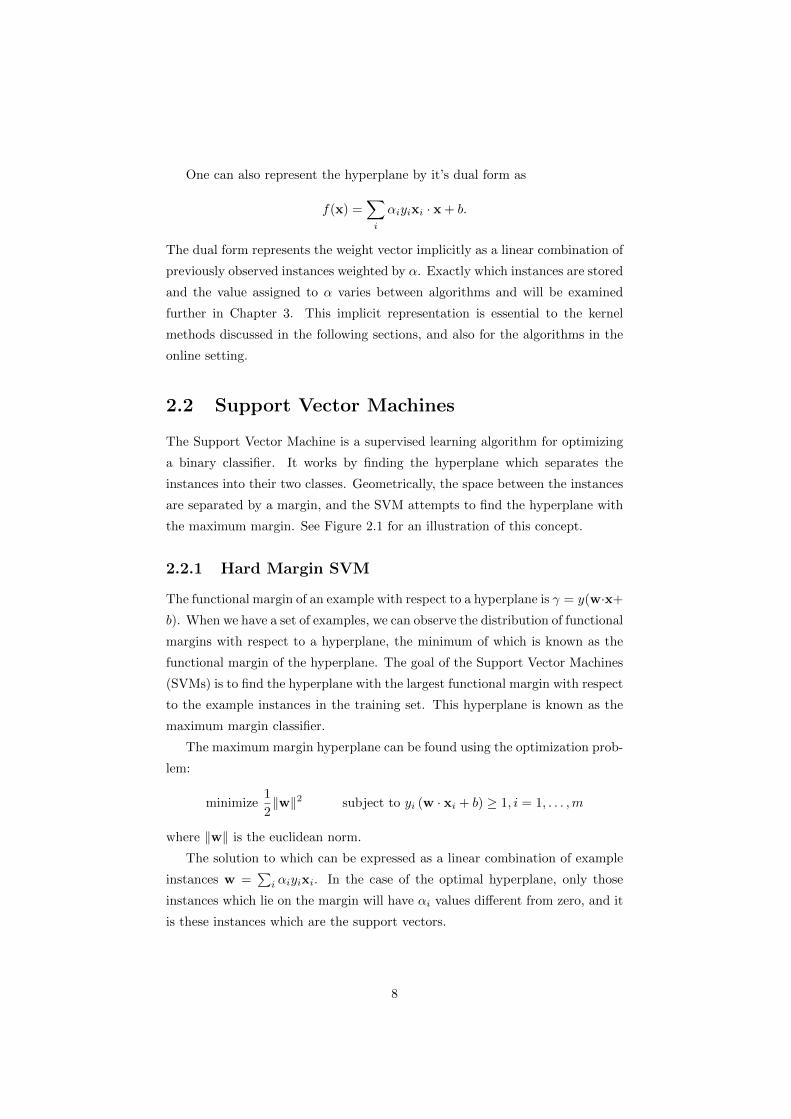
One can also represent the hyperplane by it’s dual form as

f(x) =∑i

αiyixi · x + b.

The dual form represents the weight vector implicitly as a linear combination of

previously observed instances weighted by α. Exactly which instances are stored

and the value assigned to α varies between algorithms and will be examined

further in Chapter 3. This implicit representation is essential to the kernel

methods discussed in the following sections, and also for the algorithms in the

online setting.

2.2 Support Vector Machines

The Support Vector Machine is a supervised learning algorithm for optimizing

a binary classifier. It works by finding the hyperplane which separates the

instances into their two classes. Geometrically, the space between the instances

are separated by a margin, and the SVM attempts to find the hyperplane with

the maximum margin. See Figure 2.1 for an illustration of this concept.

2.2.1 Hard Margin SVM

The functional margin of an example with respect to a hyperplane is γ = y(w·x+

b). When we have a set of examples, we can observe the distribution of functional

margins with respect to a hyperplane, the minimum of which is known as the

functional margin of the hyperplane. The goal of the Support Vector Machines

(SVMs) is to find the hyperplane with the largest functional margin with respect

to the example instances in the training set. This hyperplane is known as the

maximum margin classifier.

The maximum margin hyperplane can be found using the optimization prob-

lem:

minimize1

2‖w‖2 subject to yi (w · xi + b) ≥ 1, i = 1, . . . ,m

where ‖w‖ is the euclidean norm.

The solution to which can be expressed as a linear combination of example

instances w =∑i αiyixi. In the case of the optimal hyperplane, only those

instances which lie on the margin will have αi values different from zero, and it

is these instances which are the support vectors.

8

Figure 2.1: The maximum margin classifier for a set of linearly separable train-

ing data. The set of points which lie on the margin are referred to as the support

vectors.

Note: This figure depicts the geometric margin of the hyperplane and assumes

that the weight vector and bias term are normalized.

9

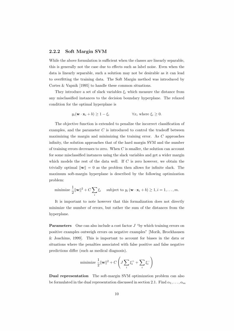
2.2.2 Soft Margin SVM

While the above formulation is sufficient when the classes are linearly separable,

this is generally not the case due to effects such as label noise. Even when the

data is linearly separable, such a solution may not be desirable as it can lead

to overfitting the training data. The Soft Margin method was introduced by

Cortes & Vapnik [1995] to handle these common situations.

They introduce a set of slack variables ξi which measure the distance from

any misclassified instances to the decision boundary hyperplane. The relaxed

condition for the optimal hyperplane is

yi(w · xi + b) ≥ 1− ξi ∀xi where ξi ≥ 0.

The objective function is extended to penalize the incorrect classification of

examples, and the parameter C is introduced to control the tradeoff between

maximizing the margin and minimizing the training error. As C approaches

infinity, the solution approaches that of the hard margin SVM and the number

of training errors decreases to zero. When C is smaller, the solution can account

for some misclassified instances using the slack variables and get a wider margin

which models the rest of the data well. If C is zero however, we obtain the

trivially optimal ‖w‖ = 0 as the problem then allows for infinite slack. The

maximum soft-margin hyperplane is described by the following optimization

problem:

minimize1

2‖w‖2 + C

∑i

ξi subject to yi (w · xi + b) ≥ 1, i = 1, . . . ,m.

It is important to note however that this formalization does not directly

minimize the number of errors, but rather the sum of the distances from the

hyperplane.

Parameters One can also include a cost factor J “by which training errors on

positive examples outweigh errors on negative examples” [Morik, Brockhausen

& Joachims, 1999]. This is important to account for biases in the data or

situations where the penalties associated with false positive and false negative

predictions differ (such as medical diagnosis).

minimize1

2‖w‖2 + C

(J∑i

ξ+i +

∑i

ξ−i

)

Dual representation The soft-margin SVM optimization problem can also

be formulated in the dual representation discussed in section 2.1. Find α1, . . . , αm

10

such thatm∑i=1

αi −1

2

m∑i,j=1

yiyjαiαj

(xi · xj +

1

Cδij

)is maximized and

αi ≥ 0,∀i = 1, . . .m

m∑i=1

yiαi = 0

It is this dual representation that allowed for the adoption of kernel methods

as discussed below.

2.3 Kernel Methods

By examining the SVM dual problem, it can be seen that the gradient of the

hyperplane w is stored implicitly as a linear combination of inner products

between support vectors.

We call a function K on two objects a kernel if it can be shown that it is

an inner product in some feature space H. We write the function mapping a

classifiable object o into the feature space vector x as φ(o) = x.

f(o) = w × φ(o) + b = 0

The so called ‘kernel trick’ lies in the fact that we can rewrite the hyperplane

defining the decision boundary as

f(x) =

(∑i

yiαiφ(oi)

)· φ(o) + b =

∑i

yiαiφ(oi) · φ(o) + b

The kernel function associated with the mapping function φ is

K(oi, o) = 〈φ(oi) · φ(o)〉

and so we can compute the classification of any instance without having to apply

the mapping φ directly.

f(x) =∑i

yiαiK(oi, o) + b

This allows for the use of kernels with potentially infinite dimensional im-

plicit feature spaces.

11

2.4 Online Learning

While online learning techniques have been studied since the introduction of the

Perceptron in 1958, they suffered a loss of popularity due to Minsky’s publication

criticizing that algorithm’s inability to classify data which is not linearly sepa-

rable [Minsky & Papert, 1969]. The kernel trick first published by Aizerman,

Braverman & Rozoner [1964] has been applied to the perceptron algorithm in its

dual form giving it the power to solve problems that are not linearly separable

in their native space.

The training of a support vector machine is at least quadratic in the number

of examples. Attempts have been made to create mixtures of SVMs for large

scale problems; splitting the data into subsets allow for a collection of SVMs

to be trained in parallel [Collobert, Bengio & Bengio, 2002]. Interest in online

learning methods have also been renewed to confront these types of problems,

due to their near state-of-art performance and greatly reduced computational

costs.

In the batch setting we are given two sets: a training set used to find a good

model, and a test set for evaluation. A batch mode algorithm will enumerate

over the training set (typically more than once) and fix the weight vector. This

model will then be used to evaluate on the test set. Batch methods often have

very good formal guarantees if the instances in the training and test sets are

drawn from the same fixed (but unknown)distribution.

In the online setting, no distinction is made between training and test sets of

instances. Learning is performed in rounds, where a single unlabelled instance x

is presented to the algorithm. The online algorithm must output its prediction

of the label y before receiving the true label y. Learning proceeds incrementally

in this way until the instances are exhausted.

Algorithm 1 Online Framework

initialize classifier f1(x)

for t = 1 . . . T do

xt ← input instance

yt = ft(xt) prediction

yt ← feedback label

`(yt, yt) loss

ft+1 ← update prediction rule

end for

Because online algorithms only process one example at a time, they tend

12

to be fast and have a predictable runtime. Another benefit of their simplicity

is that they are usually straightforward to implement. The framework is very

adaptable; to define a new online learning algorithm one only needs to define

prediction and loss functions, as well as an update rule. The goal of an online

learning algorithm is to minimize the cumulative loss∑t `(yt, yt). One can also

easily apply an online algorithm in the batch setting, while the reverse is not

generally true.

These benefits aside, it is still generally understood that any given online

algorithm will not be as performant as a well designed batch algorithm.

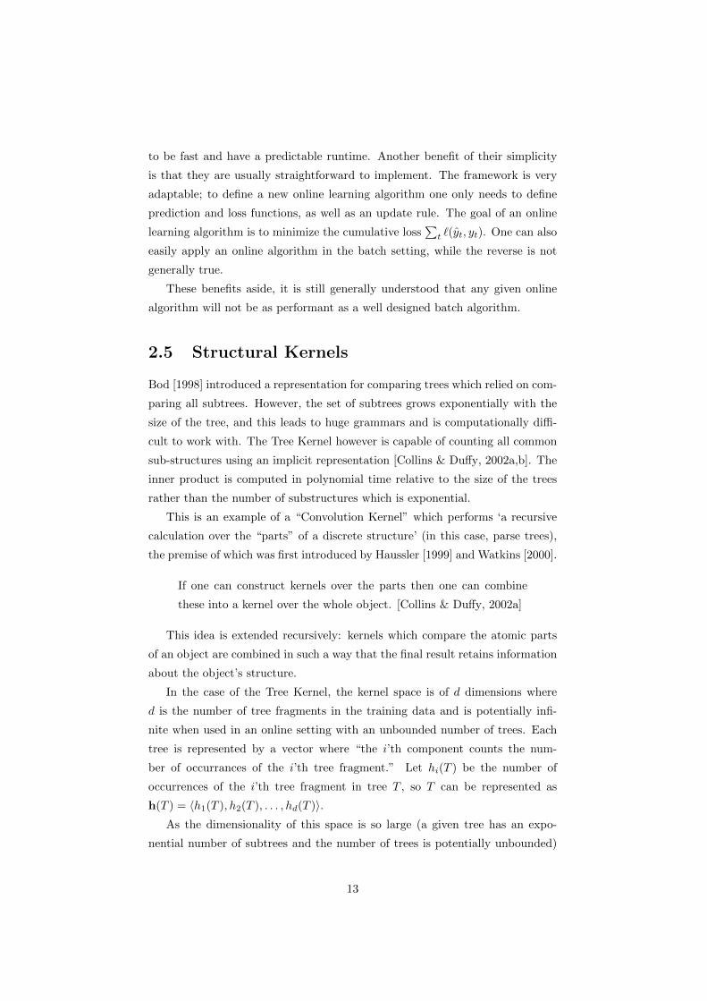
2.5 Structural Kernels

Bod [1998] introduced a representation for comparing trees which relied on com-

paring all subtrees. However, the set of subtrees grows exponentially with the

size of the tree, and this leads to huge grammars and is computationally diffi-

cult to work with. The Tree Kernel however is capable of counting all common

sub-structures using an implicit representation [Collins & Duffy, 2002a,b]. The

inner product is computed in polynomial time relative to the size of the trees

rather than the number of substructures which is exponential.

This is an example of a “Convolution Kernel” which performs ‘a recursive

calculation over the “parts” of a discrete structure’ (in this case, parse trees),

the premise of which was first introduced by Haussler [1999] and Watkins [2000].

If one can construct kernels over the parts then one can combine

these into a kernel over the whole object. [Collins & Duffy, 2002a]

This idea is extended recursively: kernels which compare the atomic parts

of an object are combined in such a way that the final result retains information

about the object’s structure.

In the case of the Tree Kernel, the kernel space is of d dimensions where

d is the number of tree fragments in the training data and is potentially infi-

nite when used in an online setting with an unbounded number of trees. Each

tree is represented by a vector where “the i’th component counts the num-

ber of occurrances of the i’th tree fragment.” Let hi(T ) be the number of

occurrences of the i’th tree fragment in tree T , so T can be represented as

h(T ) = 〈h1(T ), h2(T ), . . . , hd(T )〉.As the dimensionality of this space is so large (a given tree has an expo-

nential number of subtrees and the number of trees is potentially unbounded)

13

Collins and Duffy developed the Tree Kernel algorithm in such a way so that

its computational complexity does not depend on d.

K(T1, T2) = h(T1) · h(T2)

=

d∑i

hi(x1)hi(x2)

=

d∑i

( ∑n1∈N1

Ii(n1)

)( ∑n2∈N2

Ii(n2)

)

=∑n1∈N1

∑n2∈N2

d∑i

Ii(n1)Ii(n2)

Where Ii(n) is an indicator function equal to 1 if fragment i is left-most at

node n, and ∆(n1, n2) =∑i Ii(n1)Ii(n2) counts the number of common subtrees

rooted in nodes n1 and n2. This can be recursively defined as follows:

∆(n1, n2) =

0 if n1 6= n2

1 if n1 = n2 and are pre-terminals

nc(n1)∏j=1

(1 + ∆(ch(n1, j), ch(n2, j))) otherwise.

Where nc(n) is the number of children of n, and since the productions at n1

and n2 are the same, nc(n1) = nc(n2). Additionally, the function ch(n, j) gives

the j’th child of node n.

Collin’s and Duffy also introduce a λ parameter (0 < λ ≤ 1) to reduce the

weight of larger tree fragments by augmenting each case with a multiplication

with λ. The recursive calls result in smaller weights for larger trees, effectively

normalizing the output.

Another suggested method for normalizing the effect of the size of tree frag-

ments is to compute the following kernel:

K ′(T1, T2) =K(T1, T2)√

K(T1, T1)K(T2, T2)

14

Chapter 3

State of the Art Online

Learning Algorithms

3.1 Unbounded Algorithms

3.1.1 Perceptron

While originally introduced as a model of information storage in the brain, the

Perceptron algorithm is a very simple linear classifier which naturally fits into

the online framework. It functions by storing a hypothesis vector w which is

initialized to zero. When presented with an unlabelled instance x, it predicts

its class y as the sign of the scalar product of the instance with the hypothesis

vector. When the actual label y is revealed, if it differs from the prediction, the

hypothesis vector is updated to include the misclassified instance w = w + yx.

If the prediction was correct, the hypothesis remains unchanged. This process

is repeated for each example.

y = sign(w · x)

w =

m∑i=0

yxi

The Perceptron can be easily adapted to a batch learning framework by

running the algorithm repeatedly through the training set. This is typically done

until it finds a hypothesis vector which correctly classifies the entire training set,

which is then used to predict the labels of the instances in the test set.

Block (1962), Novikoff (1962) and Minsky and Papert (1969)

have shown that if the data are linearly separable, then the percep-

15

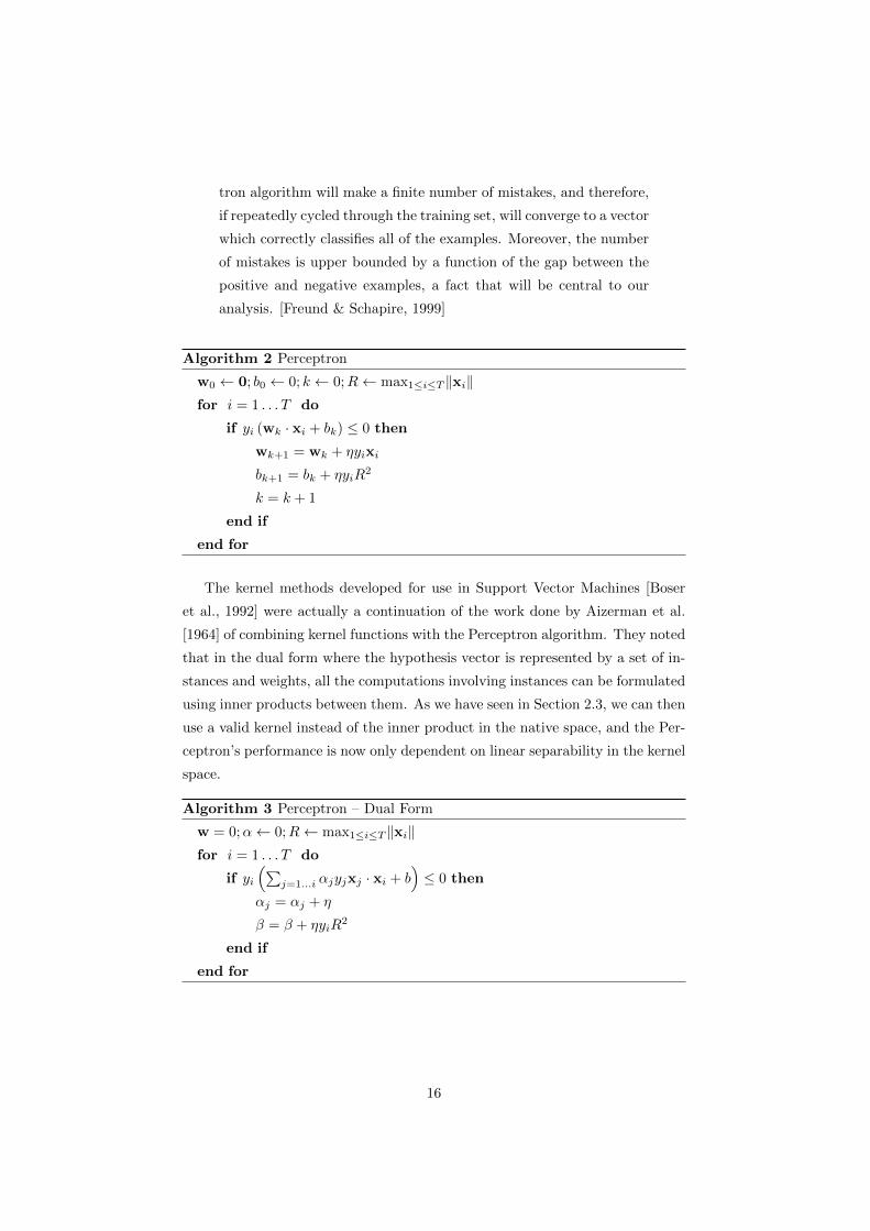
tron algorithm will make a finite number of mistakes, and therefore,

if repeatedly cycled through the training set, will converge to a vector

which correctly classifies all of the examples. Moreover, the number

of mistakes is upper bounded by a function of the gap between the

positive and negative examples, a fact that will be central to our

analysis. [Freund & Schapire, 1999]

Algorithm 2 Perceptron

w0 ← 0; b0 ← 0; k ← 0;R← max1≤i≤T ‖xi‖for i = 1 . . . T do

if yi (wk · xi + bk) ≤ 0 then

wk+1 = wk + ηyixi

bk+1 = bk + ηyiR2

k = k + 1

end if

end for

The kernel methods developed for use in Support Vector Machines [Boser

et al., 1992] were actually a continuation of the work done by Aizerman et al.

[1964] of combining kernel functions with the Perceptron algorithm. They noted

that in the dual form where the hypothesis vector is represented by a set of in-

stances and weights, all the computations involving instances can be formulated

using inner products between them. As we have seen in Section 2.3, we can then

use a valid kernel instead of the inner product in the native space, and the Per-

ceptron’s performance is now only dependent on linear separability in the kernel

space.

Algorithm 3 Perceptron – Dual Form

w = 0;α← 0;R← max1≤i≤T ‖xi‖for i = 1 . . . T do

if yi

(∑j=1...i αjyjxj · xi + b

)≤ 0 then

αj = αj + η

β = β + ηyiR2

end if

end for

16

3.1.2 Averaged Perceptron

The main idea behind the Voted and Averaged Perceptron algorithms devel-

oped by Freund & Schapire [1999] is that by averaging the output of many

models we protect against overfitting. The algorithm maintains a history of

the prediction vectors v generated after every mistake, the number of mistaken

predictions made so far (and equivalently, the number of vectors stored in the

model) is denoted by k. Additionally, the number of iterations this prediction

vector “survives” without making a mistake is counted and used as that vec-

tor’s weight in the majority vote. The intuition being that the number of correct

classifications is indicative of the quality of the vector and “better” vectors have

a larger weight in the final decision.

While Freund & Schapire describe their algorithm in the batch setting as a

“deterministic leave-one-out conversion of the online perception algorithm,” the

bounds proven for the voted-perceptron’s performance apply when the number

of training epochs is one. In other words, after seeing every training example

only once, or equivalently: the online setting.

Voted Perceptron Let vi be the prediction vector computed for mistake i,

and ci be its weight (the number of examples presented since the last misclas-

sification). Then the output prediction of the voted-perceptron when presented

with an instance x is

y =

k∑i=1

ci sign (vi · x) ,

where the inner product can be computed as

vk · x =

k−1∑j=1

yij(xij · x

),

allowing the storage of v in an implicit form as a set of instances. Furthermore,

it can be computed incrementally taking advantage of the relation vj+1 · x =

vj · x + yij(xij · x

), and use a kernel function K by replacing xij · x with

K(xij ,x

). By using this dual form, we can obtain the history of prediction

vectors from the set of stored instances. The Perceptron model need only be

augmented by the vote count ci for each stored instance.

The update step however, is very different from the standard Perceptron.

An update occurs after every instance, not only for those which the prediction

was wrong. The output of the most recent prediction vector is compared with

the true label. If correct the value of ck is incremented, if not the new instance

is added to the model.

17

Algorithm 4 Voted Perceptron

w = 0;α← 0; k ← 0

for i = 1 . . . T do

// output voted prediction

y =∑kj=1 cj sign (vj · xi)

// update if most recent prediction vector is wrong

if yi (vk · xi) ≤ 0 then

vk+1 = vk + yixi

ck+1 = 1

k = k + 1

else

ck = ck + 1

end if

end for

While the bias term is notably missing from their algorithm, this problem is

sidestepped by the use of a polynomial kernel which augments the feature space

to allow for finding hyperplanes which do not intersect with the origin.

K(a,b) = (1 + a · b)d

Averaged Perceptron The Averaged Perceptron [Freund & Schapire, 1999]

functions in the same manner as the Voted Perceptron, and varies only in how

the weighted prediction is computed. Rather than counting the number of

positive or negative predictions, the predictions are additionally weighted by

their confidence.

y = sign

(k∑i=1

ci (vi · x)

)Freund and Schapire also present a normalized version of the Averaged Per-

ceptron,

y = sign

(k∑i=1

ci

(vi · x||vi||

))However, they note that the performance difference between the two methods

are always minor. In the experiments presented in this thesis will examine the

performance of the unnormalized Averaged Perceptron variant.

Extensions Carvalho & Cohen [2006] explain how this averaging technique

can be “trivially applied to any mistake-driven online algorithm” and do so.

18

Their experiments show favourable results when applying averaging to tasks

outside of the Natural Language Processing domain, however within this domain

this technique seems to reduce performance.

3.1.3 Passive Aggressive

The Passive Aggressive family of algorithms [Crammer, Dekel, Keshet, Shalev-

Shwartz & Singer, 2006] are another example of mistake-driven additive-update

online algorithms. However, it does not limit the definition of “mistake” to cases

where an example was incorrectly labeled. The goal of the Passive Aggressive

algorithm (PA) is not simply a positive margin, but a large one in order to

predict with high confidence. It uses the following hinge-loss function,

` (w; (x, y)) =

{0 y(w · x) ≥ 1

1− y(w · x) otherwise.

Whenever the margin of a prediction is less than one (they note that this

choice of threshold is “rather arbitrary”), the Passive Aggressive algorithm per-

forms its update as follows,

wt+1 = wt + τtytxt.

The update rule must strike a balance between the amount of progress it

makes and retaining the information previously learned. This tradeoff was first

formalized by Helmbold, Kivinen & Warmuth [1999]. Progress, as Crammer

et al. have defined it for this family of algorithms, is made by modifying the

hypothesis such that it classifies the new instance with a sufficiently large mar-

gin.

Crammer et al. provide three different formulations for the value of τt. The

first variant, called simply PA is defined as

τt =`t‖xt‖2

.

This technique works well with linearly separable data. However, the occur-

rence of a mislabeled example almost guarantees that the problem is no longer

linearly separable. By employing such an aggressive update step the PA al-

gorithm makes itself susceptible to such label noise. When presented with a

mislabeled example, the updated weight vector will likely cause prediction mis-

takes on subsequent examples. As such, PA-I and PA-II are extensions to the

original algorithm to deal with this kind of problem.

19

PA-I and PA-II Inspired by Vapnik’s soft-margin support vector machine

classifiers, Crammer et al. introduce a slack parameter ξ to their objective func-

tion and an aggressiveness parameter C which controls its influence. In PA-I,

the update function scales linearly with ξ, while in PA-II it scales quadratically.

wt+1 = arg minw∈Rn

1

2‖w −wt‖2 + Cξ s.t. `(w; (xt, yt)) ≤ ξ and ξ ≥ 0 (PA-I)

wt+1 = arg minw∈Rn

1

2‖w −wt‖2 + Cξ2 s.t. `(w; (xt, yt)) ≤ ξ (PA-II)

The update rule for these two algorithms share the same closed form as PA

with τ defined as follows,

τt = min

{C,

`t‖xt‖2

}(PA-I)

τt =`t

‖xt‖2 + 12C

(PA-II)

By testing with synthetic data sets, they show that PA-I and PA-II are

indeed more robust to both instance noise and label noise.

3.2 Budgeted Algorithms

The algorithms above are guaranteed to make only a finite number of mistakes

if the data presented to them are linearly separable. However if this is not the

case, given an infinite stream of data such algorithms will make an unbounded

number of mistakes. Each such mistake results in another example being added

to the model, resulting in a model of unbounded size.

Obviously this can be a problem as any physical implementation of these

algorithms must run on a machine with finite memory. After processing a

sufficiently large quantity of examples, the stored model will exhaust its available

resources and the program will crash. This limitation is not in the spirit of online

learning.

Furthermore, as the size of these models grow, so does the computational

time needed to predict the class of each new unlabelled example. If their size is

unbounded, new predictions will eventually grind to a halt.

A number of algorithms have adopted a fixed limit on the size of their model,

typically referred to as the algorithm’s “budget.” The simplest of any such bud-

geted online algorithms is called the Stoptron, introduced by Orabona, Keshet

& Caputo [2008] as a baseline budgeted algorithm. The Stoptron functions in

20

the exact same manner as the Perceptron, however once the budget is reached

it simply stops storing new examples.

Other initial attempts at staying within the budget while still learning from

new examples used various heuristics. For example, the Randomized Budget

Perceptron [Cavallanti, Cesa-Bianchi & Gentile, 2007] begins discarding a sup-

port vector at random to make room for new examples once the budget is

reached.

3.2.1 Forgetron

The forgetron is an attempt made at continuous learning by replacing the oldest

examples when the budget B is reached. It uses the concept of shrinking the

significance of every stored example at each step such that when one needs to

remove an example, one can do so without significantly affecting the hypothesis

vector. It was the first such budgeted algorithm to offer a relative mistake

bound.

When a prediction mistake occurs, the instance is added to the model as in

the Perceptron. An additional value σ is stored for every instance in the model,

and initialized to 1 for newly added examples. After increasing the size of the

model

I ′t = It ∪ {t} f ′t = ft + ytK (xt, ·) ,

the shrinking coefficient φ is computed and the shrinking step applies it to every

instance in the model

f ′′t = φtf′t σi,t+1 = φtσi,t

reducing their effect on the hypothesis. Due to the recurring nature of this

update, the oldest instances in the model will have the smallest value of σ and

therefore the smallest effect on the hypothesis. After the shrinking step, if the

algorithm is over budget the oldest stored instance is removed

It+1 = I ′t \ {rt} ft+1 =∑i∈It+1

σi,t+1yiK(xi, ·)

Forgetron For the simplest of their presented shrinking mechanisms they de-

rive the constant U from the allocated budget B. This constant is used to

bound the norm of the hyperplane function, which allows for their proof that

the Forgetron is competitive with any hypothesis whose norm is also within

these bounds. Their choice of φ for the Forgetron provides a balance between

21

attenuating the influence of older examples and the damage caused to the hy-

pothesis.

φt = min

{(B + 1)

− 12(B+1) ,

U

‖f ′t‖

}

U =1

4

√(B + 1)

log (B + 1)

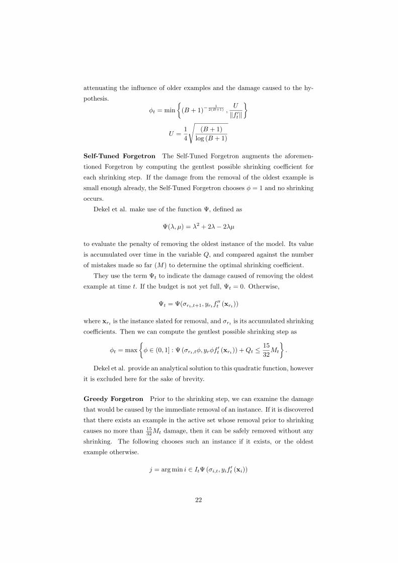
Self-Tuned Forgetron The Self-Tuned Forgetron augments the aforemen-

tioned Forgetron by computing the gentlest possible shrinking coefficient for

each shrinking step. If the damage from the removal of the oldest example is

small enough already, the Self-Tuned Forgetron chooses φ = 1 and no shrinking

occurs.

Dekel et al. make use of the function Ψ, defined as

Ψ(λ, µ) = λ2 + 2λ− 2λµ

to evaluate the penalty of removing the oldest instance of the model. Its value

is accumulated over time in the variable Q, and compared against the number

of mistakes made so far (M) to determine the optimal shrinking coefficient.

They use the term Ψt to indicate the damage caused of removing the oldest

example at time t. If the budget is not yet full, Ψt = 0. Otherwise,

Ψt = Ψ(σrt,t+1, yrtf′′t (xrt))

where xrt is the instance slated for removal, and σrt is its accumulated shrinking

coefficients. Then we can compute the gentlest possible shrinking step as

φt = max

{φ ∈ (0, 1] : Ψ (σrt,tφ, yrφf

′t (xrt)) +Qt ≤

15

32Mt

}.

Dekel et al. provide an analytical solution to this quadratic function, however

it is excluded here for the sake of brevity.

Greedy Forgetron Prior to the shrinking step, we can examine the damage

that would be caused by the immediate removal of an instance. If it is discovered

that there exists an example in the active set whose removal prior to shrinking

causes no more than 1532Mt damage, then it can be safely removed without any

shrinking. The following chooses such an instance if it exists, or the oldest

example otherwise.

j = arg min i ∈ ItΨ (σi,t, yif′t (xi))

22

rt =

{j if Ψ (σj,t, yjf

′t (xj)) ≤ 15

32

min It otherwise

The shrinking step is then performed as in the Self-Tuned Forgetron.

While this version of the algorithm is not limited to removing the oldest

example of the model, Dekel et al. note that as the size of the stored model

increases, the Greedy Forgetron tends to leave noisy examples in the model. As

such, the literature treats the Self-Tuned Forgetron as the best algorithm from

this family and it is this one which will be examined in Chapters 4 & 5.

3.2.2 Projectron

Orabona, Keshet & Caputo [2008] use a technique pioneered for the improve-

ment of Support Vector Machine solutions by Downs, Gates & Masters [2001]

to reduce the size of the support set (the set of active examples in the model)

without changing the hypothesis. Rather than having a fixed budget however,

the Projectron algorithm allows the user to set an input parameter that trades

off between model sparseness and accuracy.

Upon making a mistake, if the new instance can be represented as a linear

combination of the existing support set (xt =∑t−1i=1 dixi) it is not added to the

model. Instead of adding it directly, the coefficients of the existing support set

are updated to include the new instance, that is, αi = yi + ytdi. If however,

the new instance is linearly independent from the support set, it is added with

αt = yt as usual.

While this technique does reduce the size of the support set without chang-

ing the hypothesis at all, it can still lead to infinitely large support sets given an

infinite dimensional kernel, Orabona et al. employ the following solution by con-

structing two new hypotheses. The temporal hypothesis f ′t is simply the result

of adding the instance to the support set as usual. The projected hypothesis f ′′t

is the projection of f ′t onto the space spanned by the previous support set St−1.

If norm of the distance between the two hypotheses is below some threshold the

projected hypothesis is adopted, otherwise the temporal hypothesis is used.

This threshold is referred to as the model sparseness parameter η. If η is

equal to zero, the Projectron algorithm behaves exactly as the classical percep-

tron. As the value of η increases, the algorithm trades precision for sparseness.

They show that their strategy ensures that the size of the support set is finite,

regardless of the dimensionality of the kernel space. Their proof however, does

not state that the size of the support set can be estimated before training.

Orabona et al. also prove a performance bound that shows the Projectron

23

is slightly worse than the Perceptron. If η = 0 they have the same bound, and

its degradation is related to 11−η‖g‖ , where g is an arbitrary hypothesis.

The Projectron++ algorithm extends the Projectron by including an update

step for when the new observation is correctly classified but only with a small

margin. This mirrors the Passive-Aggressive family of algorithms improvements

upon the Perceptron. However, the margin update step is only applied when the

new instance can be projected onto the existing support set. A new instance

correctly classified but with low confidence is never directly appended to the

model (the “temporal hypothesis” as described for the error update step). While

this would improve the classification rate, it does so by greatly increasing the size

of the support set. The presented performance bound for the Projectron++ is

closely related to that of PA-I, with degradation related to η. The Projectron++

algorithm is the first budgeted online learning algorithm to outperform the

Perceptron and we examine its performance in the following Chapters.

24

Chapter 4

Method for the Empirical

Comparison of Algorithms

4.1 Implementation Details

This work provides an implementation of several state of the art online learning

algorithms as part of the SVM-Light-TK software package [Moschitti, 2006].

This library is written in the C programming language. Care was taken to write

the learning algorithms in an object oriented fashion by using virtual function

pointer tables to emulate classes. The strategy design pattern [Gamma, Helm,

Johnson & Vlissides, 1995] was also followed to allow different algorithms to

be substituted at runtime depending on the users request. To achieve this,

each algorithm provides an implementation for the functions in the following

code listing which the svm online.c algorithm calls without knowledge of the

underlying algorithm or its implementation.

Listing 4.1: Excerpt of learning algorithm.h defining the common interface

// v i r t u a l f unc t i ons

double pred ic t example ( LearningAlgorithm ∗ , DOC∗ doc ) ;

void l earn example ( LearningAlgorithm ∗ , DOC∗ doc , double t a r g e t ) ;

void conso l i da t e mode l ( LearningAlgorithm ∗) ;

void dest roy ( LearningAlgorithm ∗) ;

// s t a t i c he l p e r func t i ons

void noop ( LearningAlgorithm ∗) ;

LearningAlgorithm ∗ a l g o r i t h m c o n s t r u c t o r (ONLINE PARM∗ , MODEL∗) ;

25

While some algorithms leverage advanced data structures during their on-

line learning, the final models are consolidated into the format expected by

SVM-Light-TK so that the svm classify command can load them without fur-

ther modification. The only exception is for storing the Voted and Averaged

Perceptron models. In these cases, an integer for each instance in the model

is needed to represent the number of votes they get during classification. This

list of integers is appended to the end of the model file and svm classify was

modified to look for this extra data. If a list of votes is present, it calls the

appropriate weighted classification function.

4.2 Hyperparameter Tuning

In order to select the optimal hyperparameters for a given learning algorithm,

one typically performs a search over the possible values and evaluates the re-

sulting models on a validation set (a subset of the training set). Attempting to

ensure these evaluations generalize to the final test set, one can perform n-fold

cross validation by evaluating n complimentary training and validation subsets.

However, the hyperparameters for the algorithms under investigation in this

thesis are not suited to this manner of tuning, as accuracy is trivially optimized

at the expense of model size. For example, by setting the Projectron’s sparsity

parameter η equal to zero we obtain performance equivalent to the Perceptron

(or similar to PA-I in the case of Projectron++). Increasing this value increases

the model’s sparsity and would thus lead to a decrease in prediction accuracy.

Similarly, the aggressiveness parameter C behaves similarly to C in soft margin

SVMs. Setting it to infinity reduces PA-I to the ‘hard margin’ Passive Aggres-

sive algorithm, while setting it to zero allows for the trivially optimal ‖w‖. In

practice, C has been shown to tradeoff between the learning rate and the final

accuracy.

In the literature, these parameters are chosen somewhat arbitrarily. In an

attempt to fairly compare algorithms, we elected to adopt the same values

each algorithm’s authors present. The aggressiveness parameter C for the PA-I

algorithm was chosen to be equal to 1 as in [Orabona et al., 2008] which results

in an update that is comparable to the basic Perceptron. For the Projectron++,

η was set to 0.1 as in [Orabona, Keshet & Caputo, 2009].

26

4.3 Single-pass Evaluation

Due to the very nature of the online algorithms, the order in which the training

data is presented has an impact on the resulting model. As such, all of the

experiments presented herein were performed by training against five different

permutations of the training set.

One of the strengths of bounded memory online learning algorithms is their

applicability to continuous streams of data. When performing classification in

realtime there is no clear separation between training and test sets, and as such

no specific time when performing an additional pass over previous instances is

appropriate.

4.4 Comparing Online to Batch Mode SVMs

The ‘leave-one-out’ method for the transformation of online learning algorithms

to batch learning algorithms developed by Helmbold & Warmuth [1995] was

adapted into the voted perceptron algorithm [Freund & Schapire, 1999].

While Freund & Schapire observe that using the Voted and Averaged Per-

ceptron algorithms show improvements in performance after multiple passes

through the training set (epochs), they “do not have a theoretical explanation

for the improvement in performance following the first epoch.”

Carvalho & Cohen [2006] found that this conversion technique (which was

also applied to other online algorithms including Passive Aggressive I) improved

performance when only performing a single pass through the training data, but

this improvement was not apparent when the task was from the NLP domain.

While novel, their study of single-pass online learning did not include the use

of kernel functions. This thesis attempts to improve over their evaluation by

applying structural kernels to NLP tasks where the classes have a better chance

at being linearly separable, compared to using linear kernels over examples

represented by bags-of-words.

4.5 Experimental Procedure

In this thesis we have chosen datasets with clearly defined training and test sets.

In our experiments, the online algorithms are trained using a single pass over

the training set. At this point, their models are fixed and their performance

is evaluated over the test set. This procedure allows for the direct comparison

27

between single-pass online learning algorithms and batch-mode algorithms such

as the SVM.

Additionally, we present recordings of the online algorithms’ performance

taken throughout the training stage. These plots show how the online learning

algorithms behave as they are presented with novel instances, and are meant to

reveal their behaviour in the setting of continuous data. As such, they are not

directly comparable to batch-mode or multiple epoch algorithms.

4.6 Performance Measure

Rather than simply relying on Accuracy ( correctly classifiedtotal examples ) which can be a de-

ceptive metric when the number of positive and negative examples are skewed,

this thesis presents its results using the F1-measure which provides a balanced

view of both precision and recall in the test set.

Precision =true positives

true positives + false positives

Recall =true positives

true positives + false negatives

F1 = 2 · Precision ·RecallPrecision+Recall

The sole exception to this is in the case of multiclassifiers which we examine

in section 6.1. Since these models have more classes than simply positive and

negative, the F1 approach is not appropriate. For this reason we measure the

multiclassifier’s performance using its Accuracy.

28

Chapter 5

Feature-vector Kernel

Experiments

For the experiments described in this chapter, two generic kernels were ex-

amined: an inhomogeneous polynomial kernel and the Gaussian radial basis

function.

Polynomial Kernel

k(xi,xj) = (xi · xj + 1)d

The hyperparameter d sets the degree of the polynomial expansion. The

implicit feature space obtained when using the polynomial kernel includes di-

mensions for each monomial up to degree d. This can be seen as a method of

feature conjunction.

Gaussian radial basis function

k(xi,xj) = exp(−γ‖xi − xj‖2

)= exp (−γ (xi · xi − 2 · xi · xj + xj · xj))

The implicit feature space corresponding to the Gaussian radial basis func-

tion is one of infinite dimensions. The hyperparameter γ (sometimes expressed

as 1σ2 ) controls the smoothness of the decision boundary and the area of influence

of individual support vectors.

29

5.1 Synthetic Dataset

The synthetic datasets used in this thesis were constructed in the same man-

ner as described in [Crammer et al., 2006; Dekel et al., 2008; Orabona et al.,

2008, 2009]. Positive examples were sampled from a two-dimensional Gaussian

distribution with a mean of (1, 1) and the following covariance matrix:[0.2 0

0 2

]

Negative examples were sampled from a Gaussian distribution with a mean of

(−1,−1) and the same covariance matrix. Label noise was added by flipping

each label with probability p = 0.1.

Ten training sets of 10,000 instances each were generated along with a test

set also containing 10,000 instances. Positive and negative instances were gen-

erated with equal probability. Each online algorithm was trained using a single

pass over each of the training sets resulting in ten separate models. These re-

sulting models were each tasked with predicting the labels of the test set without

updating, the results of which were averaged and are presented below.

5.2 Synthetic Dataset Experimental Results

The test results after single-pass training are listed in Table 5.1. In it, we observe

that the SVM results in the best performance while having a runtime orders of

magnitudes greater than any of the online learning algorithms which treat the

data with a single pass. The SVM model size is also quite large, second only to

PA-I.

The averaged perceptron shows great improvement over the standard per-

ceptron at this task, both in its F1 score on the test set as well as requiring far

fewer support vectors in the model.

The Projectron++ also managed to outperform PA-I, which is interesting

as it is theoretically upper bounded by PA-I’s performance. Also interesting is

that the Projectron++ attains this level of performance with only 10 support

vectors in the model. This probably speaks to the simplicity of the underlying

data, but it demonstrates markedly more space efficient models than all the

other examined algorithms. Furthermore, with such a small model, the runtime

required to train the Projectron++ is vastly shorter than any other algorithm.

As expected, performance degrades as we restrict the size of the budget

available to the Forgetron. These budget restrictions also decrease the runtime

30

Algorithm F1 Accuracy SV Runtime (s)

SVM 89.21 ± 0.25 89.19 ± 0.27 3054.80 ± 81.85 33.89 ± 3.19

Perceptron 73.45 ± 13.42 68.81 ± 14.53 2949.50 ± 706.23 1.86 ± 0.38

Averaged 88.99 ± 0.31 88.98 ± 0.32 1961.20 ± 51.99 1.28 ± 0.04

PA-I 76.00 ± 9.85 76.04 ± 8.41 3617.00 ± 93.16 2.24 ± 0.06

Projectron++ 81.58 ± 13.36 81.11 ± 14.82 10.20 ± 0.42 0.03 ± 0.00

Forgetron1000 65.90 ± 20.99 64.63 ± 12.14 1000 1.20 ± 0.07

Forgetron500 53.26 ± 28.37 57.20 ± 9.37 500 0.69 ± 0.02

Table 5.1: Single-pass performance using polynomial kernel of degree 3 on the

synthetic dataset. Online algorithms were trained on a single pass over the

training dataset before being fixed and tested. This procedure was repeated

using 10 random permutations of the data. The mean and standard deviation

between the 10 models are listed. SV indicates the size of the support set of

the final model after training. Runtime indicates the cpu-seconds required for

training.

required for training, as we observe in the more extreme case of the Projec-

tron++.

We also note that the Accuracy and F1 measures are very similar in this

example. This is due to the balance between positive and negative examples,

an artifact of its construction as described in the previous section.

5.3 Adult Dataset

The Adult dataset from the UCI Machine Learning Repository consists of 32,561

training and 16,281 testing exampes. The task is to predict whether a given

household has an income greater than $50,000.

Each datum provides 14 attributes of a household’s census form, eight cat-

egorical attributes and six continuous. The continuous attributes have been

discretized to result in a total of 123 binary attributes. This preprocessing

was first performed by Platt [1999] and is available in SVM-Light format from

http://www.csie.ntu.edu.tw/~cjlin/libsvmtools/datasets/.

As above, the algorithms were trained using a single pass over the training

set before their models are fixed. Throughout the training however, we recorded

the model’s performance on the data instances it had been presented thus far.

For this dataset, a Gaussian radial basis function kernel was selected and

tuned with γ = 0.04 (σ2 = 25). This configuration was chosen in order to

31

Algorithm F1 Accuracy SV Runtime (s)

SVM 67.64 ± 0.02 83.36 ± 0.01 13056.60 ± 4.28 330.98 ± 6.20

Perceptron 51.24 ± 28.65 80.46 ± 3.22 6819.00 ± 33.08 73.56 ± 0.63

Averaged 42.87 ± 12.76 82.11 ± 1.84 6757.20 ± 51.91 76.30 ± 1.25

PA-I 51.50 ± 16.24 80.53 ± 3.31 12985.00 ± 46.44 134.87 ± 0.92

Projectron++ 53.52 ± 13.45 79.60 ± 4.10 2009.80 ± 12.93 204.08 ± 3.19

Forgetron3000 47.77 ± 17.66 74.07 ± 7.79 3000 41.12 ± 1.19

Forgetron1500 34.38 ± 31.34 76.20 ± 4.12 1500 17.78 ± 0.17

Table 5.2: Single-pass performance using Gaussian kernel γ = 0.04 on the Adult

dataset. Algorithms were trained on 5 different permutations of the training set

before the models were fixed. SV indicates the size of the support set of the final

model after training. Runtime indicates the cpu-seconds required for training.

match the kernel used in experiments performed in [Orabona et al., 2008], while

providing a more in-depth look at the results including how the algorithms’

performance progressed over time, and the complexity of the models produced.

In their study, Orabona et al. present the accuracy of the Projectron on this

dataset. However, due to the un-balanced nature of this dataset (24% of the

instances have positive labels), it is important to examine the F-measure as it

takes both precision and recall into account. In order to train an SVM in this

situation, an appropriate cost factor must be chosen to tune the weight of errors

on positive examples versus errors on negative examples. Initial experimentation

resulted in choosing a value of 2.5 for this hyperparameter.

5.4 Adult Dataset Experimental Results

Figure 5.1 plots the performance during the online pass through one of the five

permutations of the training set. Similarly, figures 5.2 and 5.3 show the size of

the model and the cumulative time elapsed during training respectively. The

results of using the fixed models to predict the labels of the test set are presented

in Table 5.2.

We observe in Table 5.2 that similarly to the synthetic dataset, the SVM

demonstrates the highest performance at the expense of the longest runtime

by far. PA-I stores almost twice as many support vectors as the Perceptron for

little gain in performance. The Projectron++ algorithm however, demonstrates

the best performance of all the online algorithms on this task and does so with

far fewer support vectors in its model. While its test performance is good with a

32

very sparse model, is important to note however that its time complexity during

training is even greater than PA-I, and approaches that of the SVM.

The Averaged Perceptron actually performs worse than the Perceptron in

the final test, contrary to the suggestion by Carvalho & Cohen [2006] that voting

improves performance in non-NLP tasks. Their study, however only examined

the use of the inner product between instances (linear kernel).

During training however, the Averaged Perceptron is shown to be very per-

formant in Figure 5.1. By making fewer mistakes than the Perceptron, it stores

fewer support vectors and requires less computations to predict and update as

reflected in Figures 5.2 and 5.3 respectively.

The budget cutoffs in the Forgetron algorithm can clearly be seen as the

horizontal lines in Figure 5.2 and the transition to linear growth of time in Figure

5.3. It is at these points (roughly 20% and 45% of the training instances) where

their performance diverges from the Perceptron in Figure 5.1, as expected. All

the other online algorithms show polynomial growth in runtime. In descending

order they are: Projectron++, PA-I, Perceptron, and Averaged.

33

0

20

40

60

80

100

0 1 2 3 4 5 6 7 8 9 10

F1

Per

form

ance

Percentage of Instances

PerceptronAveraged

PA-IProjectron++Forgetron1,500

Forgetron3,000

(a) Online performance on first 10% of instances

0

20

40

60

80

100

0 10 20 30 40 50 60 70 80 90 100

F1

Per

form

ance

Percentage of Instances

PerceptronAveraged

PA-IProjectron++Forgetron1,500

Forgetron3,000

(b) Online performance over all instances

Figure 5.1: Online performance during Adult9 training using a Gaussian kernel with γ =

0.04. Where 100% of the Instances corresponds to the set of 32,562 training instances. These

learning curves show the cumulative performance of the algorithm as it processes a single

permutation of the training dataset.

34

0

2000

4000

6000

8000

10000

12000

14000

0 10 20 30 40 50 60 70 80 90 100

Su

pp

ort

Vec

tors

Percentage of Instances

PerceptronAveraged

PA-IProjectron++Forgetron1,500

Forgetron3,000

Figure 5.2: Growth of support set during Adult9 training using a Gaussian

kernel with γ = 0.04. Where 100% of the Instances corresponds to the set of

32,562 training instances.

35

0

50

100

150

200

250

0 10 20 30 40 50 60 70 80 90 100

Cu

mu

lati

veT

ime

(s)

Percentage of Instances

PerceptronAveraged

PA-IProjectron++Forgetron1,500

Forgetron3,000

Figure 5.3: Cumulative runtime during Adult9 training using a Gaussian kernel

with γ = 0.04. Where 100% of the Instances corresponds to the set of 32,562

training instances.

36

Chapter 6

Structural Kernel

Experiments

The evaluation presented in this thesis is novel in its inclusion of structured

kernels. The Syntactic Tree Kernel developed by Collins & Duffy [2002a] for

evaluating natural language is applied to the Question Classification and Se-

mantic Role Labeling tasks.

6.1 Question Classification

The question classification task is a multi-class decision problem, where each

question belongs to one of 6 classes: Abbreviation, Description, Entity, Human,

Location, or Numeric. While each of these classes have sub-classes such as date,

money, or weight for the Numeric category, these have been discarded for these

experiments.

The data for this problem consists of a training set of 5483 questions and

a test set of 500 questions from http://cogcomp.cs.illinois.edu/Data/QA/

QC/.

We implement the multi-classifier in the same manner as [Moschitti, Quar-

teroni, Basili & Manandhar, 2007] in order for our results to be directly compa-

rable1. Initially one binary classifier is trained for each of the potential classes.

The training data for each of these classifiers has been transformed in a ONE-

vs-ALL scheme, where the one label for the desired class identifying positive

1While Orabona et al. [Orabona et al., 2009] provide a framework for structure learning

using the Projectron algorithm, we elected to use the same setup for all of the examined

algorithms

37

examples and all the remaining labels considered negative. This scheme has

been used successfully for Question Classification in particular by Moschitti

et al. [2007] and defended as a valid approach in general by Rifkin & Klautau

[2004].

After training each class specific binary classifier using a single pass through

the data and fixing the model, we can evaluate the algorithm’s performance on

the test set. Each test instance is presented to and classified by each of the

6 binary classifiers. The final output label is obtained by selecting the binary

classifier with the greatest confidence in a positive classification. This training

and testing procedure was performed five times using different permutations of

the training data.

To compare against SVM, we present the results of both an untuned model

as well as one with which the cost-factor values for each binary classifier were

chosen according to the best results obtained by Moschitti et al. [2007]. This

model is referred to as SVMtuned.

6.2 Question Classification Experimental Results

Table 6.2 shows each algorithm’s final performance on the multi-classification

task, averaged between the five independent models trained on different permu-

tations of the training set. Intermediate results can be seen in table 6.1 which

shows the performance of each of the six binary classifiers.

While both the multi-class SVMs are clearly superior, this experiment shows

the viability of obtaining performance approaching the state-of-the-art using

single-pass online learning algorithms in both multi-class problems and in the

NLP domain using structural kernels.

The strongest online model for the multi-classification task was created by

the PA-I algorithm, followed by the Averaged Perceptron and the Projectron++.

In some of the binary tasks we observe that the online algorithms occasionally

outperform the untuned SVM (Entity, Location, and Numeric specifically.

38

Ab

bre

via

tion

Des

crip

tion

Enti

tyH

um

an

Loca

tion

Nu

mer

ic

SV

Mtu

ned

84.2

1±

0.00

94.7

8±

0.0

080.4

3±

0.0

087.5

0±

0.0

082.5

8±

0.0

089.8

6±

0.0

0

SV

M80

.00±

0.00

96.0

0±

0.0

063.8

9±

0.0

088.1

4±

0.0

077.6

1±

0.0

080.4

2±

0.0

0

Per

cep

tron

72.1

3±

7.37

85.0

0±

10.6

054.4

6±

13.7

779.0

6±

10.4

667.5

0±

11.2

669.5

8±

8.0

6

Ave

rage

d79

.79±

5.69

93.3

1±

0.9

361.9

5±

4.6

987.0

8±

2.1

279.3

3±

3.0

079.8

4±

2.2

2

PA

-I79

.79±

5.69

91.3

8±

1.9

967.0

4±

3.3

186.9

8±

1.0

976.5

7±

5.1

581.6

0±

3.5

0

Pro

ject

ron

++

76.9

2±

6.03

87.7

3±

1.4

963.3

1±

7.0

780.8

8±

5.3

680.3

9±

5.6

579.7

1±

5.4

4

For

getr

on1000

72.1

3±

7.37

85.0

0±

10.6

044.9

6±

14.6

679.0

6±

10.4

667.5

0±

11.2

669.5

8±

8.0

6

For

getr

on750

72.1

3±

7.37

73.7

1±

15.2

236.6

6±

8.4

466.4

4±

27.8

662.3

8±

11.0

269.5

8±

8.0

6

For

getr

on500

72.1

3±

7.37

47.9

1±

25.1

331.0

2±

11.9

661.2±

15.5

660.6

1±

12.3

059.4

9±

19.9

0

Tab

le6.

1:S

ixb

inar

ycl

assi

fica

tion

task

s,on

efo

rea

chQ

Cca

tegory

.E

ach

alg

ori

thm

was

pre

sente

dw

ith

five

per

mu

tati

on

sof

the

on

e-vs-

all

trai

nin

gse

tsre

sult

ing

infi

vese

par

ate

mod

els

for

each

bin

ary

task

.A

fter

train

ing

the

mod

els

are

fixed

.T

hei

rp

erfo

rman

ceis

giv

enby

the

mea

nF

1sc

ore

ofth

efi

vem

od

els

onth

ete

stse

t.

39

Algorithm Accuracy

SVMtuned 89.00 ± 0.01

SVM 86.23 ± 0.08

Perceptron 73.47± 4.19

Averaged 82.76± 0.95

PA-I 83.43 ± 2.76

Projectron++ 81.75 ± 2.15

Forgetron1000 72.83 ± 3.80

Forgetron750 65.75 ± 6.94

Forgetron500 48.58 ± 10.26

Table 6.2: Performance of the global multi-classifiers on the question classifica-

tion task. The multi-classifiers are created by combining the six binary classifiers

whose performance is shown in Table 6.1. All models are fixed for testing. Each

test instance is presented to every classifier to predict the instance’s inclusion in

the given class. The label of the classifier with the largest confidence is selected

as the global multi-classifier’s prediction for that instance. The performance of

the five models trained on different permutations of the data are averaged and

presented here.

6.3 Boundary Classification in Semantic Role

Labeling

Automated Semantic Role Labeling (SRL) is a task that has received great at-

tention recently. Such systems require the ability to detect the word embodying

the predicate as well as the the ability to detect and classify the sequences consti-

tuting the predicate’s arguments. It has been shown that syntactic information

can effectively encode predicate-argument relationships and be leveraged for a

machine learning solution, and the Shalow Semantic Tree Kernel [Moschitti,

Pighin & Basili, 2008] has proved its ability to do just that.

The task examined herein is to discriminate between nodes which are a part

of the predicate’s argument (regardless of role) and those which are NARG

(non-argument) nodes. This Boundary Classifier (BC) is the first step before

a Role Multi-classifier (RM) would assign each example determined to be an

argument of the predicate the most appropriate label. This technique of splitting

40

node labelling into two tasks greatly reduces the computational cost as one

needs only to apply the BC to all the parse-tree nodes and the RM can ignore

irrelevant nodes. This two stage technique was first suggested by Gildea &

Jurafsky [2002] and later extended into a four step heirarchical architecture by

Moschitti, Giuglea, Coppola & Basili [2005].

The dataset is taken from the CoNLL Shared Task introduced by Carreras

& Marquez [2005] and consists of 4,463,066 examples where the predicate-

argument pairs have been manually annotated. Each example includes a syntac-

tic tree as well as linear features generated from automatic parses as detailed in

[Moschitti et al., 2008]. Approximately 5% of the corpus are positive examples.

To compare online performance against SVM, we examine the results ob-

tained by Severyn & Moschitti [2010]. They demonstrate an SVM trained on

the same 1,000,000 instances and tested against the two final sections of the cor-

pus named sec23 and sec24. We present the F1 score of the fixed online models

against each of these datasets. We made use of the same machines to run our ex-

periments (Intel R©Xenon R©2.33GHz CPU with 6Gb of RAM running the Linux

kernel 2.6.18) so that the computational time may be directly compared.

6.4 Semantic Role Labeling Experimental Re-

sults

In Figure 6.1 we see the online performance of the algorithms as they are trained

on the dataset. The PA-I algorithm demonstrates the highest level of perfor-

mance early in training (a), but is matched by the Averaged Perceptron after

approximately half of the data (500,000 instances) have been observed (b). The

Projectron++ is the next-most performant, followed by the Perceptron and the

Forgetron. It is interesting to note how the Forgetron demonstrates a sudden

loss of performance about halfway through the data, before slowly recovering to

its previous level of performance.

We observe in Figure 6.2 that the growth rate of the Projectron++ algorithm

in this case is much greater than in the previous experiments of Chapter 5. This

may be due to the high-dimensional nature of the tree kernel coupled with the

complexity of the SRL Boundary Classification problem.

The Averaged Perceptron however, demonstrates a greatly reduced support

set size compared to the Perceptron. Another interesting observation is that

while initially growing much faster, the PA-I support set slows down to the

same rate as the Perceptron after approximately 30% of the instances.

41

Severyn & Moschitti [2010] observe that training an SVM on the first mil-

lion instances of SRL task corpora takes approximately 7.5 days. While the

Projectron++ took a similar amount of time to complete its training, all the

other online algorithms were much faster to train. Their progress can be seen

in Figure 6.3, and final training times are listed in Table 6.3.

After training on one million instances, the online models were fixed and

tested against sec23 and sec24 sets, the results of which are shown in Table

6.3. We observe that the online algorithms demonstrate performance that very

closely approaches that of the SVM. Particularly successful was the Averaged

Perceptron which did so while using less than half the number of support vectors.

Algorithm Training time SV sec23 sec24

SVM 178.42 61,881 83.82 81.17

Perceptron 16.63 28,334 80.36 78.22

Averaged 15.50 25,559 83.35 81.16

PA-I 42.52 70,412 83.03 81.05

Projectron++ 186+ 21,552+ – –

Forgetron10,000 9.97 10,000 68.33 66.53

Table 6.3: F1 performance of fixed models on two test sets. The SVM perfor-

mance is quoted from [Severyn & Moschitti, 2010]. At the time of writing, the

Projectron++ algorithm had not completed its training. Training time is listed

in hours, and SV indicates the number of support vectors in the model.

42

0

20

40

60

80

100

0 2 4 6 8 10

F1

Per

form

ance

Percentage of Instances

PerceptronAveraged

PA-IProjectron++

Forgetron10,000

(a) Online performance on first 10% of instances

0

20

40

60

80

100

0 10 20 30 40 50 60 70 80 90 100

F1

Per

form

ance

Percentage of Instances

PerceptronAveraged

PA-IProjectron++

Forgetron10,000

(b) Online performance over all instances

Figure 6.1: Online performance on the SRL Boundary Classification task.

Where 100% of the Instances corresponds to the set of one million candidate

nodes. These learning curves show the cumulative performance of each algo-

rithm as it processes the corpora.43

0

10000

20000

30000

40000

50000

60000

70000

80000

0 10 20 30 40 50 60 70 80 90 100

Su

pp

ort

Vec

tors

Percentage of Instances

PerceptronAveraged

PA-IProjectron++

Forgetron10,000

Figure 6.2: Growth of support set during SRL Boundary Classification training,

where 100% of the instances corresponds to the set of one million candidate

nodes.

44

0

10

20

30

40

50

60

0 10 20 30 40 50 60 70 80 90 100

Cu

mu

lati

veT

ime

(hou

rs)

Percentage of Instances

PerceptronAveraged

PA-IProjectron++

Forgetron10,000

Figure 6.3: Cumulative runtime during SRL Boundary Classification training,

where 100% of the instances corresponds to the set of one million candidate

nodes.

45

Chapter 7

Conclusion

Theoretically-motivated algorithms consistently outperform the heuris-

tic approach [Dekel et al., 2008]

This sentiment is mirrored in the adoption of Tree Kernels over individual

feature engineering in natural language processing tasks. Feature sets hand

tuned for specific problems cannot hope to match such generally applicable

kernels.

7.1 Summary

This thesis has investigated a number of state of the art online learning algo-

rithms for binary classifications, and examined their performance in a number

of situations.

While the Support Vector Machine demonstrates clearly superior accuracy

in almost all cases, these experiments show the viability of obtaining near state-

of-the-art performance using single-pass online learning algorithms. These algo-

rithms are able to be trained using a single pass through the training data and

as such are typically much faster to train than a Support Vector Machine for the

same problem. In fact, on the Semantic Role Labeling Boundary Classification

task the Averaged Perceptron was able to match the SVMs performance with

one third the number of support vectors and one tenth the cpu-runtime during

training.

Another important caveat is that when dealing with data with an unbalanced

number of positive and negative examples, SVMs require a tuned value for their

cost-factor hyperparameter in order to obtain good performance. While we

46

attempt to show a fair comparison between the two, the online algorithms did

not receive this kind of tuning, but still performed quite well in the face of this

kind of data.

The Perceptron, while being one of the oldest linear classifiers demonstrates

good performance. The Averaged Perceptron leverages the whole set of mod-

els generated during training, giving each a weighted vote proportional to their

performance. This technique helps protect against over-fitting, and can be im-

plemented with very little additional overhead. The Passive Aggressive family

of algorithms build upon the Perceptron’s successes by not only updating when

a classification error is made, but also when the confidence of a correct classifi-

cation is too low. Their approach generates accurate models at the expense of

storing many support vectors, especially when dealing with noisy data.

These techniques perform well, but their models can grow unboundedly when

presented with a continuous stream of data. Many techniques have arisen to

address this shortcoming.

The Forgetron algorithm is a theoretically well founded approach to learning

under the constraint of a fixed budget of support vectors, however its accuracy

is upper bounded by that of the Perceptron as it discards data while its time

and space complexity are much lower. The Projectron algorithm does not heed

a fixed budget, but stores new instances as a linear combination of existing ones

when possible. This guarantees the size of the model to be finite even in the

face of continuous data. The Projectron++ goes a step further by taking the

same aggressive update approach as the PA algorithms, giving it accuracy upper

bounded by PA while working within a fixed budget.

The maintenance of the inverse Gram matrix (K−1 in Orabona et al. [2008])

means that while the Projectron algorithm stores far fewer support vectors it

still requires a long computational time.

The Projectron derives its savings from ensuring a small set of support vec-

tors. However, in the Semantic Role Labeling Boundary Classification experi-

ments it was observed that its support set grew much faster than in the other

situations, and as such resulted in very long processing times. Further investi-

gation into the causes behind this are required to fully evaluate the Projectron’s

effectiveness when applied to problems using structured kernels.

The results found herein suggest that high-accuracy online learning algo-

rithms are possible and that they can serve some purposes that are not well

suited to SVMs, such as when presented with extremely large datasets. These al-

gorithms and techniques have proven themselves not only in traditional feature-

47

vector kernel spaces, but also when using extremely high-dimensional structural

kernels. This observation is heartening as many problems in the natural lan-

guage processing domain are well described by annotated parse trees, and often

involve massive amounts of data which can pose a problem for support vector

machines.

7.2 Critical Analysis

One of the main drawbacks of the presented empirical evaluation was in the

choices of hyperparameters. In the face of unbalanced ratios of positive and

negative examples in the dataset, it is sometimes necessary to choose an ap-

propriate value for the cost-factor when training an SVM in order to obtain

non-trivial results. For the Adult dataset a very rough search was used to find

an acceptable value. However, similar tuning was not performed for the online

algorithms.

In fact, the hyperparameters for the online algorithms were chosen based on

suggestions in the literature and not changed. This was particularly troublesome

for the Projectron++ algorithm when presented with the SRL dataset. Using

a fixed value of η = 0.1 resulted in a very dense model and very long training

time.

Orabona et al. describe a method where η can be set dynamically through-

out training. As the model accumulates support vectors and approaches a set

budget, the value of η allows fewer instances to be added to the model. This

technique is described in their paper as an attempt to make the Projectron al-

gorithm comparable with the Forgetron and it’s fixed budget. At the beginning

of each round η is set to be

η =1

2U

(2`(ft−1(xt), yt)− ‖Pt−1k(xt, ·)‖2 − 0.5

),

where the value of U is from the derivation of the Forgetron by Dekel et al.

[2008]. Given a maximum number of support vectors B, we have a maximum

value for U = 1/4√

(B + 1)/ log(B + 1).

This might have served the SRL task better, and additional experimentation

is needed to verify the Projectron’s viability in this setting.

The value of the aggressiveness parameter C for the Passive Aggressive al-

gorithm was similarly set using recommendations from the literature. However,

future work is needed to compare the effects of selecting different values for C

against the other online algorithms.

48

7.3 Future Work

The online learning framework allows for the creation of unique algorithms with

widely varying capabilities and merits further exploration. The rest of this

section describes some of the possible avenues of research that are outside the

scope of this thesis.

Forgetful Projectron While the Forgetron reduces the impact of removing

an example by gradually lowering its effect on the hypothesis over time, by

the time an instance is finally removed it is already largely forgotten. The

Projectron on the other hand, reduces the impact of removal by attempting to

store the information that would be lost as a linear combination of that which

remains. While some information can be lost in the projection into the space

spanned by the instances in memory, no observations are discarded outright.

It would be interesting to see a combination of the two approaches. Consider

the following variant to the Projectron algorithm. Instead of projecting new in-

stances onto the existing set in order to reduce the number of support vectors,

the new instance is always added. The projected hypothesis for this variant

would be created by removing the oldest stored instance and projecting it onto

the remaining support set. While potentially even more computationally expen-

sive as the inverse Gram matrix might not be able to be updated incrementally,

this variant might be able to handle datasets that exhibit concept drift while

maintaining a finite budget.

Dynamic Aggressiveness The Crammer et al. note that the value of the

aggressiveness parameter C is a tradeoff between the learning rate and the final

model performance. When C is small, the algorithm shows a slower progress

rate but ultimately reaches a higher level of performance. For large values of C

the opposite is true. They also note that “as a general rule-of-thumb, C should

be small when the data is noisy.”

It would be interesting to attempt to let the algorithm itself set the value of

C dynamically throughout learning. While early noisy examples may be added

to the support set reducing the final accuracy, techniques for maintaining a fixed

budget proposed by Wang & Vucetic [2010] could be adapted to weed them out.

This could be considered a kind of Passive Aggressive boosting technique.

49

Appendix A

SVM-Light-TK Usage

To specify the use of online algorithms, set the flag -z o.

svm_learn -z o -A perceptron datafile

To specify which online algorithm to use, set the -A flag followed by one of

the following options:

perceptron

averaged

pa

pai

paii

forgetron

tunedforgetron

greedyforgetron

projectron

projectron++

To specify the kernel to use, set the -t flag.

0: linear (default)

1: polynomial (s a*b+c)^d

2: radial basis function exp(-gamma ||a-b||^2)

3: sigmoid tanh(s a*b + c)

4: user defined kernel from kernel.h

5: combination of forest and vector sets according to W, V, S, C options

50

Bibliography

Aizerman, A., Braverman, E., & Rozoner, L. (1964). Theoretical foundations

of the potential function method in pattern recognition learning. Automation

and Remote Control, 25, 821 – 837.

Bod, R. (1998). Beyond Grammar: An experience-based theory of language.

CSLI Publications/Cambridge University Press.

Boser, B. E., Guyon, I. M., & Vapnik, V. N. (1992). A training algorithm for

optimal margin classifiers. In Proceedings of the fifth annual workshop on

Computational learning theory - COLT ’92, (pp. 144–152)., New York, New

York, USA. ACM Press.

Carreras, X. & Marquez, L. (2005). Introduction to the CoNLL-2005 shared

task: semantic role labeling. In Proceedings of the Ninth Conference on Com-

putational Natural Language Learning, (pp. 152–164).

Carvalho, V. R. & Cohen, W. W. (2006). Single-pass online learning: perfor-

mance, voting schemes and online feature selection. In Proceedings of the

12th ACM SIGKDD international conference on Knowledge discovery and

data mining, (pp. 548–553).

Cavallanti, G., Cesa-Bianchi, N., & Gentile, C. (2007). Tracking the best hyper-

plane with a simple budget Perceptron. Machine Learning, 69 (2-3), 143–167.

Collins, M. & Duffy, N. (2002a). Convolution Kernels for Natural Language.

Advances in neural information processing systems, 1, 625–632.

Collins, M. & Duffy, N. (2002b). New ranking algorithms for parsing and tag-

ging: Kernels over discrete structures, and the voted perceptron. In Proceed-

ings of the 40th Annual Meeting on Association for Computational Linguis-

tics, number July, (pp. 263–270).

51

Collobert, R., Bengio, S., & Bengio, Y. (2002). A parallel mixture of SVMs for

very large scale problems. Neural computation, 14 (5), 1105–14.

Cortes, C. & Vapnik, V. (1995). Support-vector networks. Machine Learning,

20 (3), 273–297.

Crammer, K., Dekel, O., Keshet, J., Shalev-Shwartz, S., & Singer, Y. (2006).

Online Passive-Aggressive Algorithms. The Journal of Machine Learning Re-

search, 7, 551–585.

Dekel, O., Shalev-Shwartz, S., & Singer, Y. (2008). The Forgetron: A Kernel-

Based Perceptron on a Budget. SIAM Journal on Computing, 37 (5), 1342–

1372.

Downs, T., Gates, K., & Masters, A. (2001). Exact simplification of support

vector solutions. Journal of Machine Learning Research, 2 (293-297), 85–87.

Freund, Y. & Schapire, R. E. (1999). Large Margin Classification Using the

Perceptron Algorithm.

Gamma, E., Helm, R., Johnson, R., & Vlissides, J. (1995). Design patterns:

elements of reusable object-oriented software. Addison-Wesley.

Gildea, D. & Jurafsky, D. (2002). Automatic Labeling of Semantic Roles. Com-

putational Linguistics, 28 (3), 245–288.

Haussler, D. (1999). Convolution Kernels on Discrete Structures. Technical

report, University of Santa Cruz.

Helmbold, D. P., Kivinen, J., & Warmuth, M. K. (1999). Relative loss bounds

for single neurons. IEEE transactions on neural networks, 10 (6), 1291–304.

Helmbold, D. P. & Warmuth, M. K. (1995). On Weak Learning. Journal of

Computer and System Sciences, 50 (3), 551–573.

Joachims, T. (1999). Making large-Scale SVM Learning Practical. Advances in

Kernel Methods - Support Vector Learning, 169–184.

Minsky, M. & Papert, S. (1969). Perceptrons: an introduction to computational

geometry. Cambridge, Mass.: M.I.T. Press.

Morik, K., Brockhausen, P., & Joachims, T. (1999). Combining statistical learn-

ing with a knowledge-based approach - A case study in intensive care monitor-

ing. In Proceedings of the 16th International Conference on Machine Learning.

52

Moschitti, A. (2006). Making Tree Kernels Practical for Natural Language

Learning. In Proceedings of the Eleventh International Conference on Euro-

pean Association for Computational Linguistics, Trento, Italy.

Moschitti, A., Giuglea, A.-M., Coppola, B., & Basili, R. (2005). Hierarchical

semantic role labeling. In Proceedings of the Ninth Conference on Computa-

tional Natural Language Learning, (pp. 201–204)., Ann Arbor,MI.

Moschitti, A., Pighin, D., & Basili, R. (2008). Tree Kernels for Semantic Role

Labeling. Computational Linguistics, 34 (2), 193–224.

Moschitti, A., Quarteroni, S., Basili, R., & Manandhar, S. (2007). Exploiting

syntactic and shallow semantic kernels for question / answer classification. In

Proceedings of the 45th Annual meeting of the Association for Computational

Linguistics, Prague.

Orabona, F., Keshet, J., & Caputo, B. (2008). The Projectron : a Bounded

Kernel-Based Perceptron. In Proceedings of the 25th international conference

on Machine learning, (pp. 720–727).

Orabona, F., Keshet, J., & Caputo, B. (2009). Bounded kernel-based online

learning. The Journal of Machine Learning Research, 10, 2643–2666.

Platt, J. C. (1999). Fast training of support vector machines using sequen-

tial minimal optimization. Advances in Kernel Methods, 12 (MSR-TR-98-14),

185–208.

Rifkin, R. & Klautau, A. (2004). In Defense of One-Vs-All Classification. The

Journal of Machine Learning Research, 5, 101–141.

Rosenblatt, F. (1958). The perceptron: a probabilistic model for information

storage and organization in the brain. Psychological review, 65 (6), 386–408.

Severyn, A. & Moschitti, A. (2010). Large-Scale Support Vector Learning with

Structural Kernels. In Proceedings of the 21th European Conference on Ma-

chine Learning, Barcelona, Spain.

Wang, Z. & Vucetic, S. (2010). Online Passive-Aggressive Algorithms on a

Budget. In Proceedings of the 13th International Conference on Artificial

Intelligence and Statistics, volume 9, (pp. 908–915).

Watkins, C. (2000). Dynamic Alignment Kernels. In A. Smola, P. Bartlett,

B. Schlkopf, & D. Schuurmans (Eds.), Advances in Large Margin Classifiers

(pp. 39–50). MIT Press.

53