online multi-frame blind deconvolution with super

Astronomy& Astrophysics manuscript no. aa13955-09 c© ESO 2011May 13, 2011

Online multi-frame blind deconvolutionwith super-resolution and saturation correction

M. Hirsch, S. Harmeling, S. Sra, and B. Schölkopf

Max Planck Institute for Intelligent Systems, SpemannstraSSe 38, 72076 Tübingen, Germany�

e-mail: [email protected]

Received 23 December 2009 / Accepted 21 February 2011

ABSTRACT

Astronomical images taken by ground-based telescopes suffer degradation due to atmospheric turbulence. This degradation can betackled by costly hardware-based approaches such as adaptive optics, or by sophisticated software-based methods such as luckyimaging, speckle imaging, or multi-frame deconvolution. Software-based methods process a sequence of images to reconstruct adeblurred high-quality image. However, existing approaches are limited in one or several aspects: (i) they process all images inbatch mode, which for thousands of images is prohibitive; (ii) they do not reconstruct a super-resolved image, even though an imagesequence often contains enough information; (iii) they are unable to deal with saturated pixels; and (iv) they are usually non-blind,i.e., they assume the blur kernels to be known. In this paper we present a new method for multi-frame deconvolution called online blinddeconvolution (OBD) that overcomes all these limitations simultaneously. Encouraging results on simulated and real astronomicalimages demonstrate that OBD yields deblurred images of comparable and often better quality than existing approaches.

Key words. methods: numerical – techniques: image processing – techniques: miscellaneous – atmospheric effects

1. Introduction1

Astronomical observation using ground-based telescopes is sig-2

nificantly degraded by diffraction-index fluctuations caused by3

atmospheric turbulence. This turbulence arises from local tem-4

perature and density inhomogeneities and results in a time- and5

space-variant point spread function (PSF). Often the PSF is as-6

sumed to be invariant within a short time-period and a small re-7

gion of space, called an isoplanatic patch. The coherence time8

and the size of the isoplanatic patch depend on the strength of9

the turbulence that is usually quantified by Fried’s parameter ro10

(Fried 1978) ranging between 10−20 cm for visible wavelengths11

at astronomical telescope sites. The coherence time for atmo-12

spheric turbulence is effectively frozen for images with expo-13

sure times shorter than 5−15 ms. Longer exposures effectively14

perform a time average, and thereby irretrievably wipe out high15

frequency information, making them bandlimited to angular fre-16

quencies smaller than ro/λ, where λ is the wavelength of the ob-17

served light. In contrast, short-exposures encapsulate informa-18

tion up to the diffraction-limited upper frequency bound (which19

is theoretically given by the ratio D/λwhere D denotes the diam-20

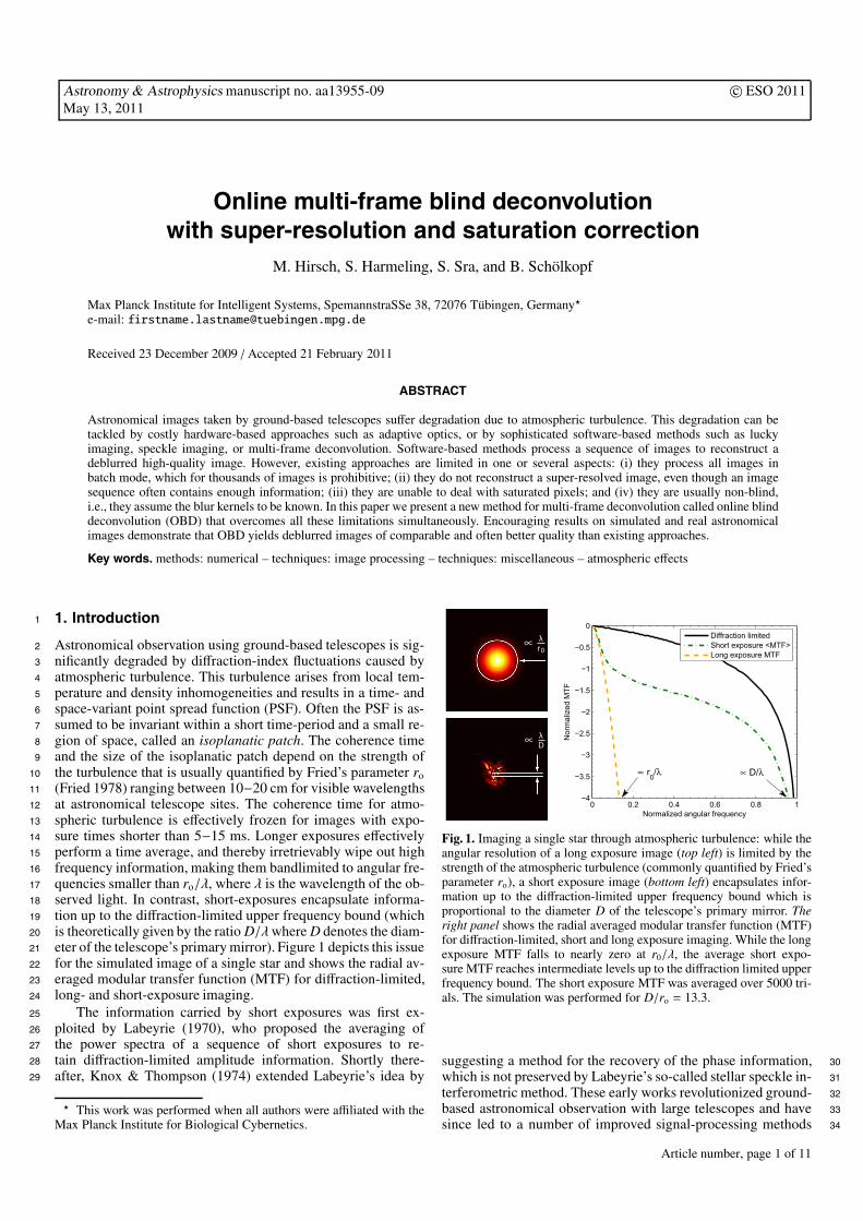
eter of the telescope’s primary mirror). Figure 1 depicts this issue21

for the simulated image of a single star and shows the radial av-22

eraged modular transfer function (MTF) for diffraction-limited,23

long- and short-exposure imaging.24

The information carried by short exposures was first ex-25

ploited by Labeyrie (1970), who proposed the averaging of26

the power spectra of a sequence of short exposures to re-27

tain diffraction-limited amplitude information. Shortly there-28

after, Knox & Thompson (1974) extended Labeyrie’s idea by29

� This work was performed when all authors were affiliated with theMax Planck Institute for Biological Cybernetics.

∝ λr0

∝ λD

0 0.2 0.4 0.6 0.8 1−4

−3.5

−3

−2.5

−2

−1.5

−1

−0.5

0

Normalized angular frequency

Nor

mal

ized

MTF

∝ r0/λ ∝ D/λ

Diffraction limitedShort exposure <MTF>Long exposure MTF

Fig. 1. Imaging a single star through atmospheric turbulence: while theangular resolution of a long exposure image (top left) is limited by thestrength of the atmospheric turbulence (commonly quantified by Fried’sparameter ro), a short exposure image (bottom left) encapsulates infor-mation up to the diffraction-limited upper frequency bound which isproportional to the diameter D of the telescope’s primary mirror. Theright panel shows the radial averaged modular transfer function (MTF)for diffraction-limited, short and long exposure imaging. While the longexposure MTF falls to nearly zero at r0/λ, the average short expo-sure MTF reaches intermediate levels up to the diffraction limited upperfrequency bound. The short exposure MTF was averaged over 5000 tri-als. The simulation was performed for D/ro = 13.3.

suggesting a method for the recovery of the phase information, 30

which is not preserved by Labeyrie’s so-called stellar speckle in- 31

terferometric method. These early works revolutionized ground- 32

based astronomical observation with large telescopes and have 33

since led to a number of improved signal-processing methods 34

Article number, page 1 of 11

(Lohmann et al. 1983; Stelzer & Ruder 2007) widely referred to1

as speckle imaging techniques.2

An alternative approach was proposed in the seminal work3

of Ayers & Dainty (1988), who presented a blind deconvo-4

lution algorithm (BD) for the problem of atmospherically de-5

graded imaging. BD recovers object information from a blurry6

and noisy observation without any additional measurement of7

the distortion. The BD of a single observation is a severely ill-8

posed problem: there are an infinite number of solutions, and9

small perturbations of the data result in large deviations in the10

estimate of the object. The ill-posedness can be alleviated to11

some degree by confining the set of solutions to physically plau-12

sible ones by introducing additional constraints or prior knowl-13

edge. Another possibility is to use multiple images or to exploit14

the partial information about wavefront distortion obtained from15

wavefront-sensor data, as used in adaptive-optics based myopic16

deconvolution algorithms.17

Since the work of Ayers & Dainty (1988) BD has grown to18

be a valuable tool in astronomical imaging and has been sub-19

ject of numerous publications. Today a plethora of algorithms20

exist that primarily differ in: (i) the data used; (ii) the a-priori21

knowledge incorporated while deblurring; and (iii) the algorith-22

mic approaches for estimating the object and its blur. For a good23

overview of BD in the domain of astronomical imaging we refer24

the reader to Kundur & Hatzinakos (1996); Molina et al. (2001);25

Pantin et al. (2007).26

Recently, electron-multiplying CCD cameras have enabled27

capturing short-time exposures with negligible noise (Mackay28

et al. 2001). This in turn has led to a new method: lucky imaging,29

which can to some degree overcome atmospherically-induced30

resolution limitations of ground-based telescopes (Law et al.31

2006; Oscoz et al. 2008; Hormuth et al. 2008). The lucky imag-32

ing idea is based on the work of Fried (1978) (who computed the33

probability of getting a lucky frame, i.e., an image recorded at a34

time instant of exceptionally good seeing). This idea proposes to35

collect only the “best” frames available in a recorded sequence.36

These “best” frames are subsequently combined to obtain a fi-37

nal image of the object. Usually, out of a thousand images, only38

a few are selected for the final reconstruction and most of the39

observed frames are discarded.40

This “wastage” can be avoided, and one can indeed use all41

the frames to obtain an improved reconstruction as we will see42

in Sect. 5.43

Methods for multiframe blind deconvolution (MFBD) aim to44

recover the image of a fixed underlying object given a sequence45

of noisy, blurry observations. Each observation has a different46

and unknown blur, which makes the deconvolution task hard.47

Previous approaches to MFBD process all observed frames48

simultaneously. Doing so limits the total number of frames that49

can be processed. We show how the computational burden can50

be greatly reduced by presenting online blind deconvolution51

(OBD)), our online algorithm that processes the input sequence52

one frame at a time. Each new frame helps to gradually improve53

the image reconstruction. This simplistic approach is not only54

natural, but also has several advantages over non-online meth-55

ods, e.g., lower resource requirements, highly competitive image56

restoration (Harmeling et al. 2009), low to moderate dependence57

on regularization or a priori information, and easy extension to58

super-resolution1 and saturation-correction.59

1 Here, super-resolution refers to techniques that are able to enhancethe resolution of a imaging system by exploiting the additional infor-mation introduced by sub-pixel shifts between multiple low resolutionimages of the same scene or object.

This paper combines preliminary work (Harmeling et al. 60

2009, 2010) in the context of astronomical imaging. In partic- 61

ular, the contributions of this paper are as follows: 62

(a) we show how to incorporate super-resolution while simulta- 63

neously performing blind deconvolution; 64

(b) we tackle saturation, a nuisance familiar to anyone who 65

works with astronomical images; 66

(c) we derive our MFBD algorithm in the framework of stochas- 67

tic gradient-descent; and 68

(d) we present results with images taken in a simple astronomer 69

setup, where one does not have access to sophisticated 70

equipment (e.g., adaptive optics), and computational re- 71

sources might be limited. 72

Before describing further details, let us put our work into per- 73

spective by briefly surveying related work. 74

2. Related work 75

MFBD. A multitude of multi-frame (or multiple-image) deblur- 76

ring papers discuss the non-blind deconvolution setup, where, 77

in addition to the image sequence the sequence of blur kernels 78

must be known as well. We do not summarize such methods here 79

because ours is a blind deconvolution method. Amongst multi- 80

ple frame blind approaches, the method of Schulz (1993) is per- 81

haps the earliest. Schulz used penalized likelihood maximiza- 82

tion based on a generalized expectation maximization (GEM) 83

framework. Closely related is Li et al. (2004), who also used 84

a GEM framework, but focused on choosing a good objective 85

function and regularizer for optimization. In contrast to our 86

work, both Schulz (1993) and Li et al. (2004) presented batch 87

algorithms that are computationally prohibitive, which greatly 88

limits the number of frames they can simultaneously process. 89

Sheppard et al. (1998) discussed the MFBD problem and 90

presented a procedure that also processes all frames at the same 91

time. They did, however, mention the possibility of incremen- 92

tal processing of frames, but gave an example only for the 93

non-blind setup. Their blind-deconvolution algorithm was based 94

on conjugate-gradients, for which they had to reparametrize 95

(e.g., x → z2 the variables to enforce nonnegativity. This 96

reparametrization has a long history in image deconvolution 97

(Biraud 1969), but numerically, the ensuing nonlinearity can be 98

damaging as it destroys the convexity of sub-problems. 99

More recently, Matson et al. (2008) also used the same non- 100

linear (x→ z2) reparametrization for solving MFBD with a par- 101

allel implementation of conjugate-gradients. Another approach 102

is that of Zhang et al. (2009), who incorporated a low-pass filter 103

into the MFBD process for suppressing noise, but again at the 104

expense of convexity. 105

Further MFBD work includes: Anconelli et al. (2006) who 106

considered methods for the reduction of boundary effects; 107

Zhulina (2006) who discussed the Ayers-Dainty algorithm; and 108

Löfdahl (2002) who permitted additional linear inequality con- 109

straints. We refer the reader to Matson et al. (2008) for even 110

more references – including those to early works – and a nice 111

summary of blind deconvolution for astronomy. Unlike our al- 112

gorithm, all the above mentioned blind deconvolution methods 113

are batch procedures; moreover none of them performs either 114

super-resolution or saturation correction. 115

Super-resolution. Numerous papers address the standard 116

super-resolution problem. For good surveys we refer the reader 117

to Park et al. (2003); Farsiu et al. (2004). However, most of these 118


M. Hirsch et al.: Online multi-frame blind deconvolution with super-resolution and saturation correction

works are based on the assumption that the blur is known, and1

only a few deal with the harder case of blind super-resolution.2

The work most closely related to ours is Šroubek et al.3

(2007), who propose a unifying framework that simultaneously4

performs blind deconvolution and super-resolution. In Šroubek5

et al. (2007, 2008) the authors show how a high-resolution image6

can be obtained from multiple blurry and noise corrupted low-7

resolution frames. However, their model assumes a priori knowl-8

edge about both the image and the blur, and Šroubek et al. (2008)9

themselves note that their method suffers from numerical insta-10

bilities for super-resolution factors larger than 2.5. In contrast,11

our approach exploits the abundance of available data, which for12

moderate noise levels does not require imposing any image or13

blur prior (except nonnegativity), leading to an overall simpler14

algorithm. Moreover, our method is computationally more effi-15

cient, since it is online.16

3. The OBD algorithm17

3.1. Problem formulation18

For simplicity of exposition, our description will focus on19

one-dimensional images and point spread functions (PSFs).20

In Appendix A we cover the generalization to two-dimensions.21

Let each observed (blurry and noisy) frame be denoted by yt,22

the “true” unknown image by x, and each unknown PSF by ft.23

Then, we use the observation model24

yt = ft ∗ x + nt, t = 1, 2, . . . , T, (1)

where ft ∗ x represents convolution (circular or non-circular),25

and nt denotes measurement noise. Further, on physical grounds26

we assume both the image x and the PSF ft to be nonnegative.27

3.2. Algorithm28

First consider the case where given the next observation yt and29

the current image estimate xt, we wish to compute the PSF ft.30

Assuming the noise nt in Eq. (1) to be Gaussian distributed with31

zero mean and incorporating nonnegativity, the PSF ft can be de-32

termined by solving a nonnegative least-squares (NNLS) prob-33

lem2. For a given observation frame yt and a current estimate xt,34

we define the loss35

�(yt; x) = minft≥0‖ yt − ft ∗ x ‖2. (2)

For a frame sequence y1, y2, . . . , yT , we aim to minimize the36

overall loss by computing the image x that solves37

minx≥0

LT (x) =1T

T∑t=1

�(yt; x). (3)

Problem (3) is not easy, because it is non-convex and its38

optimal solution requires computing both x as well as the39

PSFs f1, . . . , fT . Nevertheless, given our formulation, several40

methods could potentially be used for minimizing LT (x). For ex-41

ample, an ordinary gradient-projection scheme would be42

xt+1 = P+(xt − αt∇LT (xt)

), t = 0, 1, . . . , (4)

where P+ denotes projection onto the nonnegative orthant; xt de-43

notes the current image estimate; and αt is an appropriate step-44

size. However, when the number of frames T is large, such an45

2 This NNLS problem may be solved by various methods; we used theLBFGS-B algorithm (Byrd et al. 1995).

approach rapidly becomes computationally impractical. Hence 46

we turn to a simpler method that processes the input one frame 47

at a time. 48

3.3. Stochastic gradient descent 49

A simple and often effective method for minimizing the overall 50

loss in Eq. (3) is stochastic gradient descent (SGD). This method 51

does not process all the frames simultaneously, but at step t it 52

picks (at random) some frame y and updates the current image 53

estimate xt as 54

xt+1 = P+(xt − αt∇�(y; xt)

), (5)

where P+ and αt are as before; computing ∇�(y; xt) requires 55

solving Eq. (2). By processing only one frame at a time, 56

SGD leads to huge computational savings. However, there are 57

two main difficulties: update rule (5) converges slowly; and more 58

importantly, it is sensitive to the choice of the step-size αt; a pop- 59

ular choice is αt = β/(t0 + t), where the constants t0 and β must 60

be tuned empirically. 61

We propose a practical modification to the step-size compu- 62

tation, wherein we instead use the scaled-gradient version 63

xt+1 = P+(xt − αtS t∇�(y; xt)

), (6)

where S t is a positive-definite matrix. Also update rule (6) can be 64

shown to converge3 under appropriate restrictions on αt and S t 65

(Kushner & Yin 2003; Bottou 1998). In general, the matrix S t is 66

chosen to approximate the inverse of the Hessian of LT (x∗) for an 67

optimal x∗, thereby yielding quasi-Newton versions of SGD. But 68

a more straightforward choice is given by the diagonal matrix 69

S t = Diag((xt + ε)/(F

Tt Ft xt + ε)

), (7)

where the Diag operator maps a vector x to a diagonal matrix 70

with elements of x along its diagonal. Also note that the divi- 71

sion in (7) is element-wise, Ft is the matrix representation of 72

the PSF ft (see Appendix A), and ε > 0 is a positive constant 73

which ensures that S t remains positive definite and bounded 74

(both requirements are crucial for convergence of the method). 75

The choice (7) can be motivated with the help of auxiliary func- 76

tions (e.g., as in Harmeling et al. 2009). 77

Remark: We note in passing that if one were to use αt = 1, 78

and set ε = 0, then although convergence is no longer guaran- 79

teed, iteration (6) takes a particularly simple form, namely, 80

xt+1 = xt � (FTt y)/(F

Tt Ft xt), (8)

where � denotes the Hadamard (elementwise) product of two 81

vectors – this update may be viewed as an online version of the 82

familiar ISRA (see Daube-Witherspoon & Muehllehner 1986). 83

Note that for (7) the matrix F corresponds to the PSF f com- 84

puted via the NNLS problem (2) with y and x = xt. We call the 85

method based on iteration (6) online blind deconvolution (OBD) 86

and provide pseudo-code as Algorithm 1. We further note that 87

by assuming photon shot noise (Poisson-distributed) in Eq. (1) 88

instead of additive noise, we can also design a Richardson-Lucy 89

type iteration for solving Eq. (3). 90

3 One can show almost sure (a.s.) convergence of the objective, anda.s. convergence of the gradient to the gradient at a stationary point.


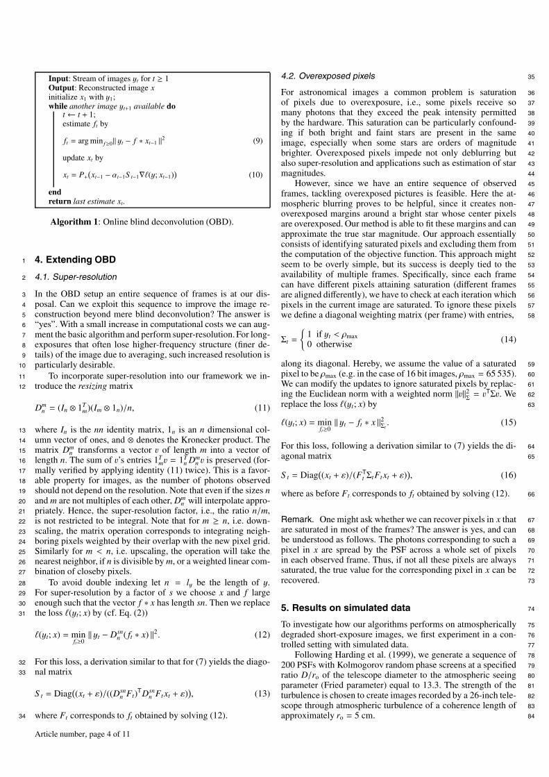
Input: Stream of images yt for t ≥ 1Output: Reconstructed image xinitialize x1 with y1;while another image yt+1 available do

t ← t + 1;estimate ft by

ft = arg min f≥0‖ yt − f ∗ xt−1 ‖2 (9)

update xt by

xt = P+(xt−1 − αt−1S t−1∇�(y; xt−1)

)(10)

endreturn last estimate xt.

Algorithm 1: Online blind deconvolution (OBD).

4. Extending OBD1

4.1. Super-resolution2

In the OBD setup an entire sequence of frames is at our dis-3

posal. Can we exploit this sequence to improve the image re-4

construction beyond mere blind deconvolution? The answer is5

“yes”. With a small increase in computational costs we can aug-6

ment the basic algorithm and perform super-resolution. For long-7

exposures that often lose higher-frequency structure (finer de-8

tails) of the image due to averaging, such increased resolution is9

particularly desirable.10

To incorporate super-resolution into our framework we in-11

troduce the resizing matrix12

Dmn = (In ⊗ 1T

m)(Im ⊗ 1n)/n, (11)

where In is the nn identity matrix, 1n is an n dimensional col-13

umn vector of ones, and ⊗ denotes the Kronecker product. The14

matrix Dmn transforms a vector v of length m into a vector of15

length n. The sum of v’s entries 1Tmv = 1T

n Dmn v is preserved (for-16

mally verified by applying identity (11) twice). This is a favor-17

able property for images, as the number of photons observed18

should not depend on the resolution. Note that even if the sizes n19

and m are not multiples of each other, Dmn will interpolate appro-20

priately. Hence, the super-resolution factor, i.e., the ratio n/m,21

is not restricted to be integral. Note that for m ≥ n, i.e. down-22

scaling, the matrix operation corresponds to integrating neigh-23

boring pixels weighted by their overlap with the new pixel grid.24

Similarly for m < n, i.e. upscaling, the operation will take the25

nearest neighbor, if n is divisible by m, or a weighted linear com-26

bination of closeby pixels.27

To avoid double indexing let n = ly be the length of y.28

For super-resolution by a factor of s we choose x and f large29

enough such that the vector f ∗ x has length sn. Then we replace30

the loss �(yt; x) by (cf. Eq. (2))31

�(yt; x) = minft≥0‖ yt − Dsn

n ( ft ∗ x) ‖2. (12)

For this loss, a derivation similar to that for (7) yields the diago-32

nal matrix33

S t = Diag((xt + ε)/((Dsn

n Ft)TDsnn Ft xt + ε)

), (13)

where Ft corresponds to ft obtained by solving (12).34

4.2. Overexposed pixels 35

For astronomical images a common problem is saturation 36

of pixels due to overexposure, i.e., some pixels receive so 37

many photons that they exceed the peak intensity permitted 38

by the hardware. This saturation can be particularly confound- 39

ing if both bright and faint stars are present in the same 40

image, especially when some stars are orders of magnitude 41

brighter. Overexposed pixels impede not only deblurring but 42

also super-resolution and applications such as estimation of star 43

magnitudes. 44

However, since we have an entire sequence of observed 45

frames, tackling overexposed pictures is feasible. Here the at- 46

mospheric blurring proves to be helpful, since it creates non- 47

overexposed margins around a bright star whose center pixels 48

are overexposed. Our method is able to fit these margins and can 49

approximate the true star magnitude. Our approach essentially 50

consists of identifying saturated pixels and excluding them from 51

the computation of the objective function. This approach might 52

seem to be overly simple, but its success is deeply tied to the 53

availability of multiple frames. Specifically, since each frame 54

can have different pixels attaining saturation (different frames 55

are aligned differently), we have to check at each iteration which 56

pixels in the current image are saturated. To ignore these pixels 57

we define a diagonal weighting matrix (per frame) with entries, 58

Σt =

{1 if yt < ρmax0 otherwise (14)

along its diagonal. Hereby, we assume the value of a saturated 59

pixel to be ρmax (e.g. in the case of 16 bit images, ρmax = 65 535). 60

We can modify the updates to ignore saturated pixels by replac- 61

ing the Euclidean norm with a weighted norm ‖v‖2Σ= vTΣv. We 62

replace the loss �(yt; x) by 63

�(yt; x) = minft≥0‖ yt − ft ∗ x ‖2Σt

. (15)

For this loss, following a derivation similar to (7) yields the di- 64

agonal matrix 65

S t = Diag((xt + ε)/(FT

t ΣtFt xt + ε)), (16)

where as before Ft corresponds to ft obtained by solving (12). 66

Remark. One might ask whether we can recover pixels in x that 67

are saturated in most of the frames? The answer is yes, and can 68

be understood as follows. The photons corresponding to such a 69

pixel in x are spread by the PSF across a whole set of pixels 70

in each observed frame. Thus, if not all these pixels are always 71

saturated, the true value for the corresponding pixel in x can be 72

recovered. 73

5. Results on simulated data 74

To investigate how our algorithms performs on atmospherically 75

degraded short-exposure images, we first experiment in a con- 76

trolled setting with simulated data. 77

Following Harding et al. (1999), we generate a sequence of 78

200 PSFs with Kolmogorov random phase screens at a specified 79

ratio D/ro of the telescope diameter to the atmospheric seeing 80

parameter (Fried parameter) equal to 13.3. The strength of the 81

turbulence is chosen to create images recorded by a 26-inch tele- 82

scope through atmospheric turbulence of a coherence length of 83

approximately ro = 5 cm. 84



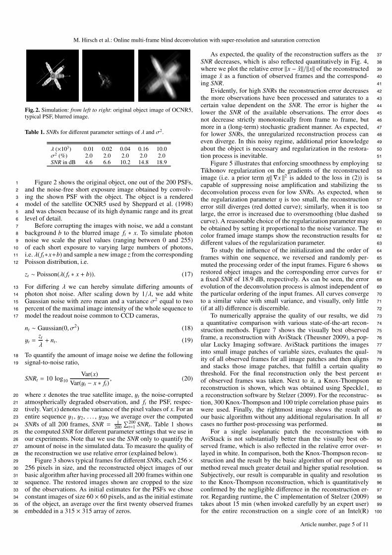
Fig. 2. Simulation: from left to right: original object image of OCNR5,typical PSF, blurred image.

Table 1. SNRs for different parameter settings of λ and σ2.

λ (×103) 0.01 0.02 0.04 0.16 10.0σ2 (%) 2.0 2.0 2.0 2.0 2.0SNR in dB 4.6 6.6 10.2 14.8 18.9

Figure 2 shows the original object, one out of the 200 PSFs,1

and the noise-free short exposure image obtained by convolv-2

ing the shown PSF with the object. The object is a rendered3

model of the satellite OCNR5 used by Sheppard et al. (1998)4

and was chosen because of its high dynamic range and its great5

level of detail.6

Before corrupting the images with noise, we add a constant7

background b to the blurred image ft ∗ x. To simulate photon8

noise we scale the pixel values (ranging between 0 and 255)9

of each short exposure to varying large numbers of photons,10

i.e. λ( ft∗x+b) and sample a new image z from the corresponding11

Poisson distribution, i.e.12

zt ∼ Poisson(λ( ft ∗ x + b)). (17)

For differing λ we can hereby simulate differing amounts of13

photon shot noise. After scaling down by 1/λ, we add white14

Gaussian noise with zero mean and a variance σ2 equal to two15

percent of the maximal image intensity of the whole sequence to16

model the readout noise common to CCD cameras,17

nt ∼ Gaussian(0, σ2) (18)

yt =zt

λ+ nt. (19)

To quantify the amount of image noise we define the following18

signal-to-noise ratio,19

SNRt = 10 log10Var(x)

Var(yt − x ∗ ft), (20)

where x denotes the true satellite image, yt the noise-corrupted20

atmospherically degraded observation, and ft the PSF, respec-21

tively. Var(x) denotes the variance of the pixel values of x. For an22

entire sequence y1, y2, . . . , y200 we average over the computed23

SNRs of all 200 frames, SNR = 1200

∑200t=1 SNRt. Table 1 shows24

the computed SNR for different parameter settings that we use in25

our experiments. Note that we use the SNR only to quantify the26

amount of noise in the simulated data. To measure the quality of27

the reconstruction we use relative error (explained below).28

Figure 3 shows typical frames for different SNRs, each 256 ×29

256 pixels in size, and the reconstructed object images of our30

basic algorithm after having processed all 200 frames within one31

sequence. The restored images shown are cropped to the size32

of the observations. As initial estimates for the PSFs we chose33

constant images of size 60 × 60 pixels, and as the initial estimate34

of the object, an average over the first twenty observed frames35

embedded in a 315 × 315 array of zeros.36

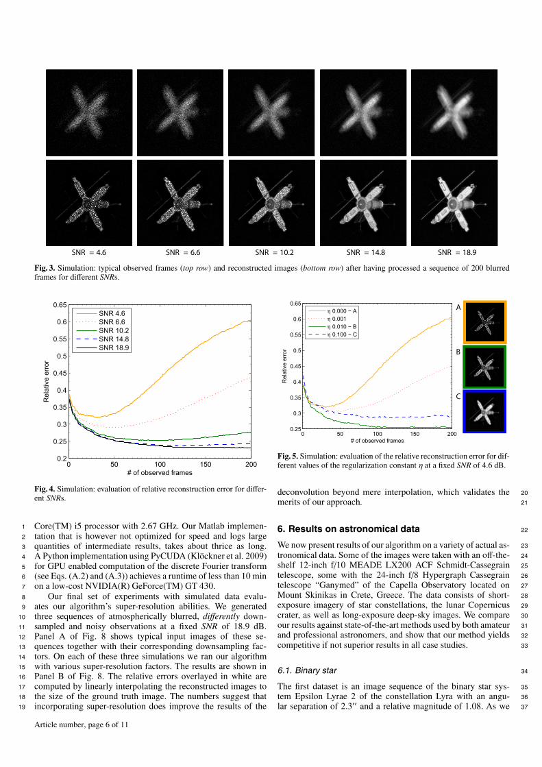
As expected, the quality of the reconstruction suffers as the 37

SNR decreases, which is also reflected quantitatively in Fig. 4, 38

where we plot the relative error ‖x − x̂‖/‖x‖ of the reconstructed 39

image x̂ as a function of observed frames and the correspond- 40

ing SNR. 41

Evidently, for high SNRs the reconstruction error decreases 42

the more observations have been processed and saturates to a 43

certain value dependent on the SNR. The error is higher the 44

lower the SNR of the available observations. The error does 45

not decrease strictly monotonically from frame to frame, but 46

more in a (long-term) stochastic gradient manner. As expected, 47

for lower SNRs, the unregularized reconstruction process can 48

even diverge. In this noisy regime, additional prior knowledge 49

about the object is necessary and regularization in the restora- 50

tion process is inevitable. 51

Figure 5 illustrates that enforcing smoothness by employing 52

Tikhonov regularization on the gradients of the reconstructed 53

image (i.e. a prior term η‖ ∇x ‖2 is added to the loss in (2)) is 54

capable of suppressing noise amplification and stabilizing the 55

deconvolution process even for low SNRs. As expected, when 56

the regularization parameter η is too small, the reconstruction 57

error still diverges (red dotted curve); similarly, when it is too 58

large, the error is increased due to oversmoothing (blue dashed 59

curve). A reasonable choice of the regularization parameter may 60

be obtained by setting it proportional to the noise variance. The 61

color framed image stamps show the reconstruction results for 62

different values of the regularization parameter. 63

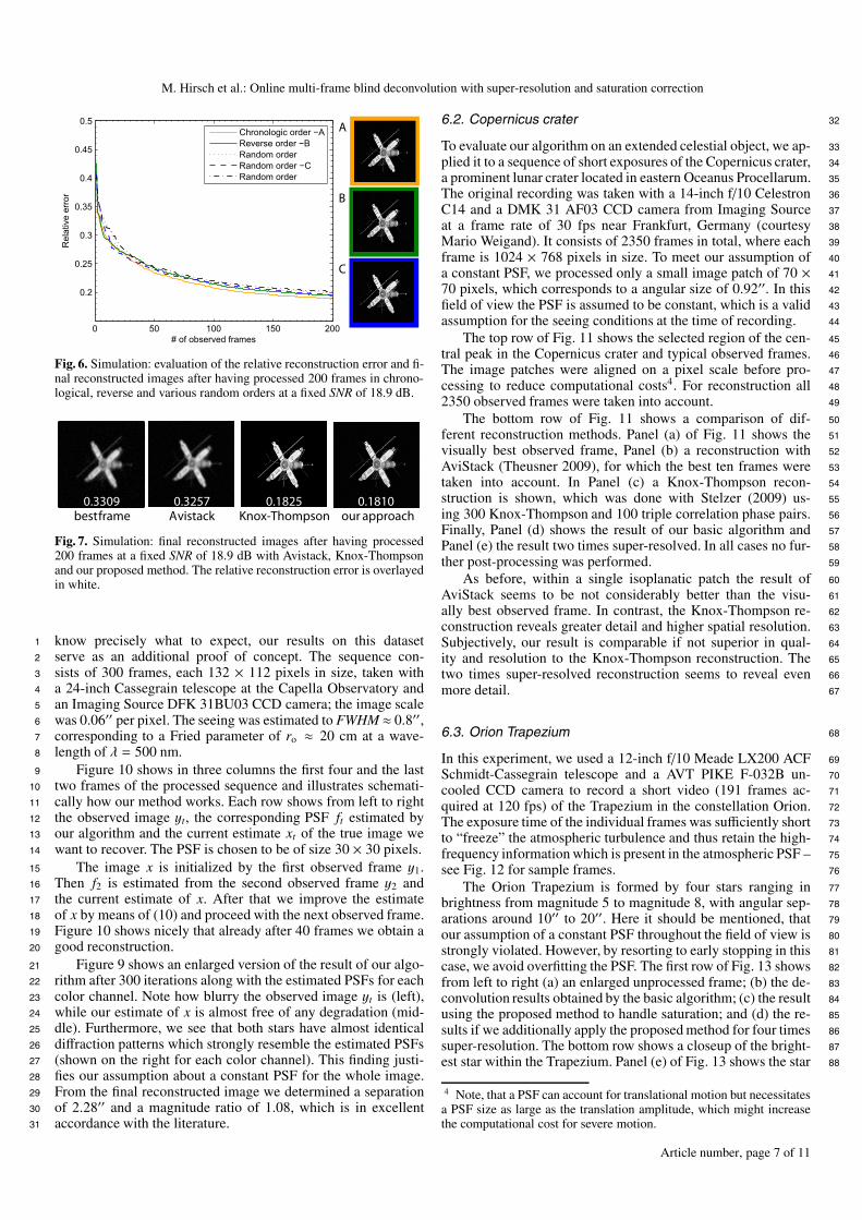
To study the influence of the initialization and the order of 64

frames within one sequence, we reversed and randomly per- 65

muted the processing order of the input frames. Figure 6 shows 66

restored object images and the corresponding error curves for 67

a fixed SNR of 18.9 dB, respectively. As can be seen, the error 68

evolution of the deconvolution process is almost independent of 69

the particular ordering of the input frames. All curves converge 70

to a similar value with small variance, and visually, only little 71

(if at all) difference is discernible. 72

To numerically appraise the quality of our results, we did 73

a quantitative comparison with various state-of-the-art recon- 74

struction methods. Figure 7 shows the visually best observed 75

frame, a reconstruction with AviStack (Theusner 2009), a pop- 76

ular Lucky Imaging software. AviStack partitions the images 77

into small image patches of variable sizes, evaluates the qual- 78

ity of all observed frames for all image patches and then aligns 79

and stacks those image patches, that fulfill a certain quality 80

threshold. For the final reconstruction only the best percent 81

of observed frames was taken. Next to it, a Knox-Thompson 82

reconstruction is shown, which was obtained using Speckle1, 83

a reconstruction software by Stelzer (2009). For the reconstruc- 84

tion, 300 Knox-Thompson and 100 triple correlation phase pairs 85

were used. Finally, the rightmost image shows the result of 86

our basic algorithm without any additional regularisation. In all 87

cases no further post-processing was performed. 88

For a single isoplanatic patch the reconstruction with 89

AviStack is not substantially better than the visually best ob- 90

served frame, which is also reflected in the relative error over- 91

layed in white. In comparison, both the Knox-Thompson recon- 92

struction and the result by the basic algorithm of our proposed 93

method reveal much greater detail and higher spatial resolution. 94

Subjectively, our result is comparable in quality and resolution 95

to the Knox-Thompson reconstruction, which is quantitatively 96

confirmed by the negligible difference in the reconstruction er- 97

ror. Regarding runtime, the C implementation of Stelzer (2009) 98

takes about 15 min (when invoked carefully by an expert user) 99

for the entire reconstruction on a single core of an Intel(R) 100


SNR = 4.6 SNR = 6.6 SNR = 10.2 SNR = 14.8 SNR = 18.9

Fig. 3. Simulation: typical observed frames (top row) and reconstructed images (bottom row) after having processed a sequence of 200 blurredframes for different SNRs.

Fig. 4. Simulation: evaluation of relative reconstruction error for differ-ent SNRs.

Core(TM) i5 processor with 2.67 GHz. Our Matlab implemen-1

tation that is however not optimized for speed and logs large2

quantities of intermediate results, takes about thrice as long.3

A Python implementation using PyCUDA (Klöckner et al. 2009)4

for GPU enabled computation of the discrete Fourier transform5

(see Eqs. (A.2) and (A.3)) achieves a runtime of less than 10 min6

on a low-cost NVIDIA(R) GeForce(TM) GT 430.7

Our final set of experiments with simulated data evalu-8

ates our algorithm’s super-resolution abilities. We generated9

three sequences of atmospherically blurred, differently down-10

sampled and noisy observations at a fixed SNR of 18.9 dB.11

Panel A of Fig. 8 shows typical input images of these se-12

quences together with their corresponding downsampling fac-13

tors. On each of these three simulations we ran our algorithm14

with various super-resolution factors. The results are shown in15

Panel B of Fig. 8. The relative errors overlayed in white are16

computed by linearly interpolating the reconstructed images to17

the size of the ground truth image. The numbers suggest that18

incorporating super-resolution does improve the results of the19

ηηηη

A

B

C

Fig. 5. Simulation: evaluation of the relative reconstruction error for dif-ferent values of the regularization constant η at a fixed SNR of 4.6 dB.

deconvolution beyond mere interpolation, which validates the 20

merits of our approach. 21

6. Results on astronomical data 22

We now present results of our algorithm on a variety of actual as- 23

tronomical data. Some of the images were taken with an off-the- 24

shelf 12-inch f/10 MEADE LX200 ACF Schmidt-Cassegrain 25

telescope, some with the 24-inch f/8 Hypergraph Cassegrain 26

telescope “Ganymed” of the Capella Observatory located on 27

Mount Skinikas in Crete, Greece. The data consists of short- 28

exposure imagery of star constellations, the lunar Copernicus 29

crater, as well as long-exposure deep-sky images. We compare 30

our results against state-of-the-art methods used by both amateur 31

and professional astronomers, and show that our method yields 32

competitive if not superior results in all case studies. 33

6.1. Binary star 34

The first dataset is an image sequence of the binary star sys- 35

tem Epsilon Lyrae 2 of the constellation Lyra with an angu- 36

lar separation of 2.3′′ and a relative magnitude of 1.08. As we 37



A

B

C

Fig. 6. Simulation: evaluation of the relative reconstruction error and fi-nal reconstructed images after having processed 200 frames in chrono-logical, reverse and various random orders at a fixed SNR of 18.9 dB.

0.3309 0.3257 0.1825 0.1810bestframe Avistack Knox-Thompson our approach

Fig. 7. Simulation: final reconstructed images after having processed200 frames at a fixed SNR of 18.9 dB with Avistack, Knox-Thompsonand our proposed method. The relative reconstruction error is overlayedin white.

know precisely what to expect, our results on this dataset1

serve as an additional proof of concept. The sequence con-2

sists of 300 frames, each 132 × 112 pixels in size, taken with3

a 24-inch Cassegrain telescope at the Capella Observatory and4

an Imaging Source DFK 31BU03 CCD camera; the image scale5

was 0.06′′ per pixel. The seeing was estimated to FWHM ≈ 0.8′′,6

corresponding to a Fried parameter of ro ≈ 20 cm at a wave-7

length of λ = 500 nm.8

Figure 10 shows in three columns the first four and the last9

two frames of the processed sequence and illustrates schemati-10

cally how our method works. Each row shows from left to right11

the observed image yt, the corresponding PSF ft estimated by12

our algorithm and the current estimate xt of the true image we13

want to recover. The PSF is chosen to be of size 30 × 30 pixels.14

The image x is initialized by the first observed frame y1.15

Then f2 is estimated from the second observed frame y2 and16

the current estimate of x. After that we improve the estimate17

of x by means of (10) and proceed with the next observed frame.18

Figure 10 shows nicely that already after 40 frames we obtain a19

good reconstruction.20

Figure 9 shows an enlarged version of the result of our algo-21

rithm after 300 iterations along with the estimated PSFs for each22

color channel. Note how blurry the observed image yt is (left),23

while our estimate of x is almost free of any degradation (mid-24

dle). Furthermore, we see that both stars have almost identical25

diffraction patterns which strongly resemble the estimated PSFs26

(shown on the right for each color channel). This finding justi-27

fies our assumption about a constant PSF for the whole image.28

From the final reconstructed image we determined a separation29

of 2.28′′ and a magnitude ratio of 1.08, which is in excellent30

accordance with the literature.31

6.2. Copernicus crater 32

To evaluate our algorithm on an extended celestial object, we ap- 33

plied it to a sequence of short exposures of the Copernicus crater, 34

a prominent lunar crater located in eastern Oceanus Procellarum. 35

The original recording was taken with a 14-inch f/10 Celestron 36

C14 and a DMK 31 AF03 CCD camera from Imaging Source 37

at a frame rate of 30 fps near Frankfurt, Germany (courtesy 38

Mario Weigand). It consists of 2350 frames in total, where each 39

frame is 1024 × 768 pixels in size. To meet our assumption of 40

a constant PSF, we processed only a small image patch of 70 × 41

70 pixels, which corresponds to a angular size of 0.92′′. In this 42

field of view the PSF is assumed to be constant, which is a valid 43

assumption for the seeing conditions at the time of recording. 44

The top row of Fig. 11 shows the selected region of the cen- 45

tral peak in the Copernicus crater and typical observed frames. 46

The image patches were aligned on a pixel scale before pro- 47

cessing to reduce computational costs4. For reconstruction all 48

2350 observed frames were taken into account. 49

The bottom row of Fig. 11 shows a comparison of dif- 50

ferent reconstruction methods. Panel (a) of Fig. 11 shows the 51

visually best observed frame, Panel (b) a reconstruction with 52

AviStack (Theusner 2009), for which the best ten frames were 53

taken into account. In Panel (c) a Knox-Thompson recon- 54

struction is shown, which was done with Stelzer (2009) us- 55

ing 300 Knox-Thompson and 100 triple correlation phase pairs. 56

Finally, Panel (d) shows the result of our basic algorithm and 57

Panel (e) the result two times super-resolved. In all cases no fur- 58

ther post-processing was performed. 59

As before, within a single isoplanatic patch the result of 60

AviStack seems to be not considerably better than the visu- 61

ally best observed frame. In contrast, the Knox-Thompson re- 62

construction reveals greater detail and higher spatial resolution. 63

Subjectively, our result is comparable if not superior in qual- 64

ity and resolution to the Knox-Thompson reconstruction. The 65

two times super-resolved reconstruction seems to reveal even 66

more detail. 67

6.3. Orion Trapezium 68

In this experiment, we used a 12-inch f/10 Meade LX200 ACF 69

Schmidt-Cassegrain telescope and a AVT PIKE F-032B un- 70

cooled CCD camera to record a short video (191 frames ac- 71

quired at 120 fps) of the Trapezium in the constellation Orion. 72

The exposure time of the individual frames was sufficiently short 73

to “freeze” the atmospheric turbulence and thus retain the high- 74

frequency information which is present in the atmospheric PSF – 75

see Fig. 12 for sample frames. 76

The Orion Trapezium is formed by four stars ranging in 77

brightness from magnitude 5 to magnitude 8, with angular sep- 78

arations around 10′′ to 20′′. Here it should be mentioned, that 79

our assumption of a constant PSF throughout the field of view is 80

strongly violated. However, by resorting to early stopping in this 81

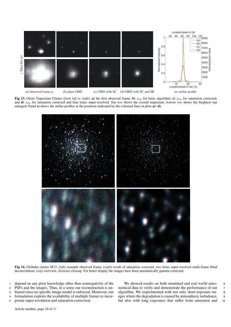
case, we avoid overfitting the PSF. The first row of Fig. 13 shows 82

from left to right (a) an enlarged unprocessed frame; (b) the de- 83

convolution results obtained by the basic algorithm; (c) the result 84

using the proposed method to handle saturation; and (d) the re- 85

sults if we additionally apply the proposed method for four times 86

super-resolution. The bottom row shows a closeup of the bright- 87

est star within the Trapezium. Panel (e) of Fig. 13 shows the star 88

4 Note, that a PSF can account for translational motion but necessitatesa PSF size as large as the translation amplitude, which might increasethe computational cost for severe motion.


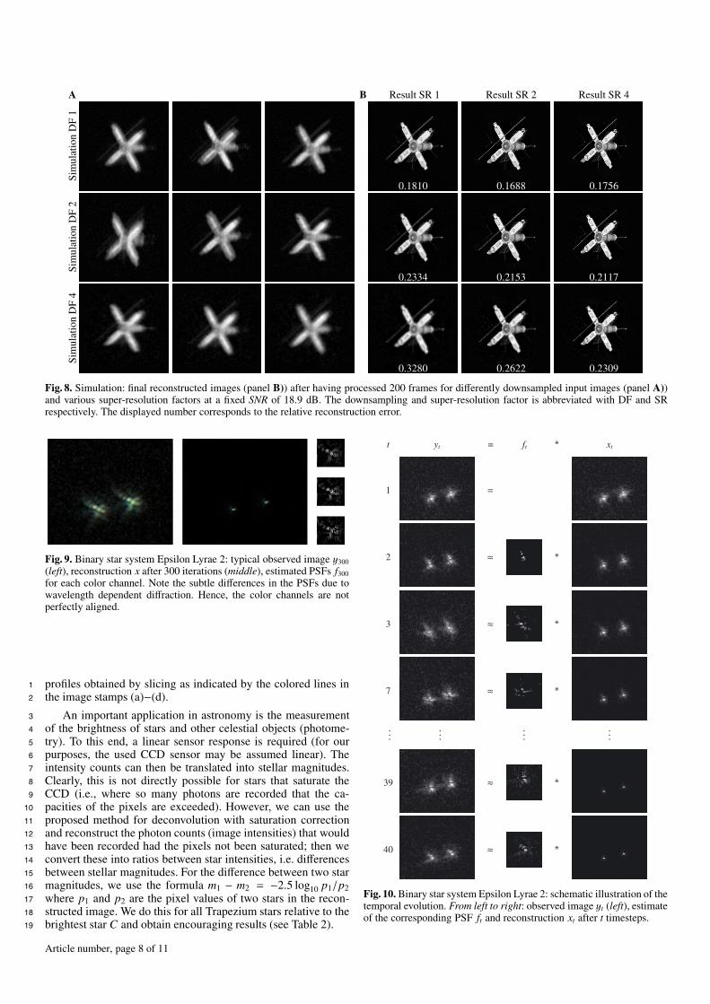
Fig. 8. Simulation: final reconstructed images (panel B)) after having processed 200 frames for differently downsampled input images (panel A))and various super-resolution factors at a fixed SNR of 18.9 dB. The downsampling and super-resolution factor is abbreviated with DF and SRrespectively. The displayed number corresponds to the relative reconstruction error.

Fig. 9. Binary star system Epsilon Lyrae 2: typical observed image y300

(left), reconstruction x after 300 iterations (middle), estimated PSFs f300

for each color channel. Note the subtle differences in the PSFs due towavelength dependent diffraction. Hence, the color channels are notperfectly aligned.

profiles obtained by slicing as indicated by the colored lines in1

the image stamps (a)−(d).2

An important application in astronomy is the measurement3

of the brightness of stars and other celestial objects (photome-4

try). To this end, a linear sensor response is required (for our5

purposes, the used CCD sensor may be assumed linear). The6

intensity counts can then be translated into stellar magnitudes.7

Clearly, this is not directly possible for stars that saturate the8

CCD (i.e., where so many photons are recorded that the ca-9

pacities of the pixels are exceeded). However, we can use the10

proposed method for deconvolution with saturation correction11

and reconstruct the photon counts (image intensities) that would12

have been recorded had the pixels not been saturated; then we13

convert these into ratios between star intensities, i.e. differences14

between stellar magnitudes. For the difference between two star15

magnitudes, we use the formula m1 − m2 = −2.5 log10 p1/p216

where p1 and p2 are the pixel values of two stars in the recon-17

structed image. We do this for all Trapezium stars relative to the18

brightest star C and obtain encouraging results (see Table 2).19

t yt = ft * xt

1 =

2 ≈ *

3 ≈ *

7 ≈ *

......

......

39 ≈ *

40 ≈ *

Fig. 10. Binary star system Epsilon Lyrae 2: schematic illustration of thetemporal evolution. From left to right: observed image yt (left), estimateof the corresponding PSF ft and reconstruction xt after t timesteps.



overview example sequence of 12 observed frames

(a) visually best frame (b) AviStack (c) Knox-Thompson (d) our approach (e) our approach2x super-resolved

Fig. 11. Copernicus Crater: top panel: full frame with extracted image patch marked by white square (left) and example sequence of 12 ob-served frames. Bottom panel: comparison of results of different reconstruction algorithms (from left to right): visually best frame, AviStack,Knox-Thompson, our approach and our approach with two times super-resolution. All image results are shown without any post-processing. Thisfigure is best viewed on screen, rather than in print.

Fig. 12. Orion Trapezium Cluster: example sequence of observed frames, y1, . . . , y10.

Table 2. True star magnitudes (note that stars A and B have variablemagnitudes), true differences to star C, and estimated difference valuesestimated after deconvolution without and with saturation correction.

Star C (ref.) A B DTrue magnitude 5.1 6.7–7.5 8.0–8.5 6.7

A–C B–C D–CTrue magnitude differences 1.6–2.4 2.9–3.4 1.6Est. diff., deconv. w/o sat. cor. 0.2936 1.4608 –0.0964Est. diff., deconv. w. sat. cor. 1.1955 2.7718 0.8124

Notes. Note that the results with saturation correction are closer to thetrue differences.

6.4. Globular cluster M131

M13 is a globular cluster in the constellation Hercules, around2

25 000 light years away, with an apparent size of around 20′.3

It contains several 100 000 stars, the brightest of which has an4

apparent magnitude of 12. Such faint stars cannot be imaged us-5

ing our equipment for short exposures; however, long exposures6

with budget equipment typically incur tracking errors, caused7

by telescope mounts that do not perfectly compensate for the8

rotation of the earth. In our case, the tracking errors induced 9

a significant motion blur in the images, which we attempted 10

to remove using the same algorithm that we used above on 11

short exposures. All raw images were recorded using a 12-inch 12

f/10 MEADE LX200 ACF Schmidt-Cassegrain telescope and a 13

Canon EOS 5D digital single lens reflex (DSLR) camera. The 14

whole sequence consists of 26 images with an exposure time 15

of 60 s each. The top row of Fig. 14 displays a long exposure 16

with motion blur (left panel and the twice super-resolved result 17

of our algorithm (right) applied to 26 motion degraded frames. 18

In the bottom row we clearly see details in our reconstructed 19

image (right) which where hidden in the recorded frames (left). 20

However, note that in the bottom right panel there appear also 21

some JPEG-like artifacts which might suggest that 26 frames 22

were not enough for two times super-resolution. 23

7. Conclusions and future work 24

In this paper, we proposed a simple, efficient, and effective mul- 25

tiframe blind deconvolution algorithm. This algorithm restores 26

an underlying static image from a stream of degraded and noisy 27

observations by processing the observations in an online fash- 28

ion. For moderate signal-to-noise ratios our algorithm does not 29


•Sl

ice

for

(e)

(a) observed frame y1 (b) plain OBD (c) OBD with SC (d) OBD with SC and SR (e) stellar profile

Fig. 13. Orion Trapezium Cluster (from left to right): a) the first observed frame; b) x191 for basic algorithm; c) x191 for saturation corrected;and d) x191 for saturation corrected and four times super-resolved. Top row shows the overall trapezium; bottom row shows the brightest starenlarged. Panel e) shows the stellar profiles at the positions indicated by the coloured lines in plots a)−d).

Fig. 14. Globular cluster M13: (left) example observed frame, (right) result of saturation corrected, two times super-resolved multi-frame blinddeconvolution; (top) overview, (bottom) closeup. For better display the images have been automatically gamma corrected.

depend on any prior knowledge other than nonnegativity of the1

PSFs and the images. Thus, in a sense our reconstruction is un-2

biased since no specific image model is enforced. Moreover, our3

formulation exploits the availability of multiple frames to incor-4

porate super-resolution and saturation-correction.5

We showed results on both simulated and real world astro- 6

nomical data to verify and demonstrate the performance of our 7

algorithm. We experimented with not only short-exposure im- 8

ages where the degradation is caused by atmospheric turbulence, 9

but also with long exposures that suffer from saturation and 10



additional blur arising from mechanical inaccuracies in the tele-1

scope mount. Our method yields results superior to or at worst2

comparable to existing frequently used reconstruction methods.3

Future work includes further building on the simplicity of4

our method to improve it to work in real-time. This goal might5

be achievable by exploiting fast graphical processing unit (GPU)6

based computing. First attempts already yielded promising re-7

sults in terms of speedup (see Sect. 5). Beyond computing im-8

provements, two other important aspects are: (i) to explore the9

spatio-temporal properties of the speckle pattern; and (ii) to in-10

corporate and investigate additional regularization within the re-11

construction process. The most challenging subject of future in-12

vestigation is to extend our method to space-varying PSFs.13

Appendix A: Implementation details14

Although in Sects. 3 and 4 we only considered vectors, one-15

dimensional convolutions, and vector-norms, all results naturally16

generalize to two-dimensional images. However, efficiently im-17

plementing the resulting algorithms for two-dimensional images18

requires some care and handling of technical details.19

A.1. Convolution as matrix-vector multiplication20

We introduced f ∗ x as the convolution, which could be either21

circular or non-circular. Due to linearity and commutativity, we22

can also use matrix-vector notation to write23

f ∗ x = Fx = X f . (A.1)

The matrices F and X are given by24

F = ITyW−1 Diag(WI f f )WIx, (A.2)

X = ITyW−1 Diag(WIxx)WI f . (A.3)

Matrix W is the discrete Fourier transform matrix, i.e., Wx is the25

Fourier transform of x. The diagonal matrix Diag(v) has vector v26

along its diagonal, while Ix, I f , and Iy are zero-padding matri-27

ces which ensure that Ixx, I f f , and Iyy have the same length.28

Different choices of the matrices lead to different margin condi-29

tion of the convolution.30

For two-dimensional images and PSFs we have to consider31

two-dimensional Fourier transforms, which can be written as32

left- and right-multiplications with W, and represented as a sin-33

gle matrix-vector multiplication using Kronecker products and34

the vectorization operator vec(x), which stacks columns of the35

two-dimensional image x into a one-dimensional vector in lexi-36

cographical order; formally,37

vec(Wx W) = (W ⊗W) vec(x), (A.4)

which follows from the identity (Horn & Johnson 1991)38

vec(A B CT) = (C ⊗ A) vec(B). (A.5)

The zero-padding operations for two-dimensional images can be39

written in a similar way.40

A.2. Resizing matrices41

The resizing matrix Dmn can be implemented efficiently using42

sparse matrices5. Resizing two-dimensional images can also be43

5 Defining for instance in Octave, D = kron(speye(m),ones(n,1)’)*kron(speye(n), ones(m,1))/m; the matrix-vectorproduct D*v will be calculated efficiently.

implemented by left- and right-multiplications: let x be an mn im- 44

age, then Dmp x (Dn

q)T is an image of size pq. Using Eq. (A.5) we 45

can write this operation as the matrix-vector product 46

vec(Dmp x (Dn

q)T) = (Dnq ⊗ Dm

p ) vec(x). (A.6)

Acknowledgements. The authors thank Hanns Ruder, Josef Pöpsel and Stefan 47Binnewies for fruitful discussions and for their generosity regarding observation 48time at the Capella Observatory. Many thanks also to Karl-Ludwig Barth (IAS) 49and Mario Weigand. We finally do thank the reviewer for a thorough review and 50valuable comments which greatly helped to improve the quality of this article. 51A Matlab demo with graphical user interface is available at http://pixel. 52kyb.tuebingen.mpg.de/obd. Corresponding author Michael Hirsch can be 53reached by e-mail at [email protected]. 54

References 55

Anconelli, B., Bertero, M., Boccacci, P., Carbillet, M., & Lanteri, H. 2006, A&A, 56448, 1217 57

Ayers, G. R., & Dainty, J. C. 1988, Opt. Lett., 13, 547 58Biraud, Y. 1969, A&A, 1, 124 59Bottou, L. 1998, in Online Learning and Neural Networks, ed. D. Saad 60

(Cambridge University Press), 9 61Byrd, R., Lu, P., Nocedal, J., & Zhu, C. 1995, SIAM J. Scientific Comp., 16, 62

1190 63Daube-Witherspoon, M. E., & Muehllehner, G. 1986, IEEE Tran. Medical 64

Imaging, 5, 61 65Farsiu, S., Robinson, D., Elad, M., & Milanfar, P. 2004, International Journal of 66

Imaging Systems and Technology, 14, 47 67Fried, D. L. 1978, J. Opt. Soc. Amer., 86 68Harding, C. M., Johnston, R. A., & Lane, R. G. 1999, Appl. Opt., 38, 2161 69Harmeling, S., Hirsch, M., Sra, S., & Schölkopf, B. 2009, in Proceedings of the 70

IEEE Conference on Computational Photography 71Harmeling, S., Sra, S., Hirsch, M., & Schölkopf, B. 2010, in Image Processing 72

(ICIP), 2010 17th IEEE International Conference on, 3313 73Hormuth, F., Hippler, S., Brandner, W., Wagner, K., & Henning, T. 2008, SPIE 74

Conf. Ser., 7014 75Horn, R. A., & Johnson, C. R. 1991, Topics in Matrix Analysis (Cambridge: 76

Cambridge University Press) 77Klöckner, A., Pinto, N., Lee, Y., et al. 2009, Performance Computing, 2009, 11 78Knox, K. T., & Thompson, B. J. 1974, ApJ, 193, L45 79Kundur, D., & Hatzinakos, D. 1996, IEEE Signal Processing Mag., 13, 43 80Kushner, H. J., & Yin, G. G. 2003, Stochastic Approximation and Recursive 81

Algorithms and Applications, 2nd edn., Applications of Mathematics 82(Springer-Verlag) 83

Labeyrie, A. 1970, A&A, 6, 85 84Law, N. M., Mackay, C. D., & Baldwin, J. E. 2006, A&A, 446, 739 85Li, B., Cao, Z., Sang, N., & Zhang, T. 2004, Electron. Lett., 1478 86Löfdahl, M. G. 2002, Proc. SPIE, 4792, 146 87Lohmann, A. W., B., G. W., & Wirnitzer. 1983, Appl. Opt., 22, 4028 88Mackay, C. D., Tubbs, R. N., Bell, R., et al. 2001, in SPIE Conf. Ser. 4306, 89

ed. M. M. Blouke, J. Canosa, & N. Sampat, 289 90Matson, C. L., Borelli, K., Jefferies, S., et al. 2008, Appl. Opt., 48 91Molina, R., Núnez, J., Cortijo, F. J., & Mateos, J. 2001, IEEE Signal Proc. Mag. 92Oscoz, A., Rebolo, R., López, R., et al. 2008, SPIE Conf. Ser., 7014 93Pantin, E., Starck, J. L., & Murtagh, F. 2007, Deconvolution and Blind 94

Deconvolution in Astronomy: Theory and Applications (CRC Press) 95Park, S., Park, M., & Kang, M. 2003, IEEE Signal Processing Magazine 96Schulz, T. J. 1993, J. Opt. Soc. Amer., 10, 1064 97Sheppard, D. G., Hunt, B. R., & Marcellin, M. W. 1998, J. Opt. Soc. Amer. A, 98

15, 978 99Šroubek, F., Cristobál, G., & Flusser, J. 2007, IEEE Tran. Imag. Proc. 100Šroubek, F., Cristobál, G., & Flusser, J. 2008, J. Phys.: Conf. Ser., 124, 012048 101

(8pp) 102Stelzer, C. 2009, Speckle1, http://www.tat.physik.uni-tuebingen.de/ 103stelzer/, version number 0.1.2 104

Stelzer, C., & Ruder, H. 2007, A&A, 475, 771 105Theusner, M. 2009, AviStack, http://www.avistack.de/index_en.html, 106

version number 1.80 107Zhang, J., Zhang, Q., & He, G. 2009, Appl. Opt., 48, 2350 108Zhulina, Y. V. 2006, Appl. Opt., 45, 7342 109


online multi-frame blind deconvolution with super

Documents