Opaque Distribution Channels for Competing Service Providers:

Posted Price vs. Name-Your-Own-Price Mechanisms*

Rachel R. Chen

Graduate School of Management

University of California at Davis

Davis, CA 95616

rachen@ucdavis.edu

Esther Gal-Or

Katz Graduate School of Business

University of Pittsburgh

Pittsburgh, PA 15260

esther@katz.pitt.edu

Paolo Roma

DICGIM - Management Research Group

Università degli Studi di Palermo

Viale delle Scienze 90128, Palermo, Italy

paolo.roma@unipa.it

*The authors are listed alphabetically and each author contributed equally to the article.

Opaque Distribution Channels for Competing Service Providers:

Posted Price vs. Name-Your-Own-Price Mechanisms

Abstract

We consider a two stage model to study the impact of different selling mechanisms of

an opaque reseller on competing travel service providers, who face both leisure and business

customers. While leisure travelers learn of their need to travel in the first stage, business

travelers learn of this need in the second stage. Business travelers have a higher willingness

to pay than leisure travelers, but their demand is stochastic. With this pattern of demand,

providers find it optimal to reserve capacity for sale in the second stage, after selling to

some leisure travelers in the first stage. After the business demand realizes, providers can

clear the remaining capacity, if any, through the opaque intermediaries in the second stage.

We find that with a single reseller, competing service providers prefer that this reseller uses

the posted price instead of the Name-Your-Own-Price mechanism. In addition, despite

the potential benefit of using an opaque reseller to price discriminate between business and

leisure customers, providers may prefer direct selling to customers without any intermediary

in the second stage. We also examine the environment with multiple opaque resellers, and

show that for competing service providers profits are the highest when selling via a single

posted price reseller.

Keywords: Competition, Name-Your-Own-Price, Posted Price, Opaque selling, Distribution

channels.

1 Introduction

In recent years, opaque retailers, exemplified by Priceline and Hotwire, have emerged as an

alternative for selling distressed inventory for service providers in the travel industry (e.g.,

airlines, hotels and car rentals). These providers typically face both leisure and business

customers. While leisure customers learn of their need for service well in advance, business

customers learn of this need much closer to the date of service delivery. Without much

flexibility to plan their travel, business customers have a much higher willingness to pay

than leisure customers, but their demand is stochastic.

With this pattern of demand, providers usually sell to leisure travelers in advance, while

reserving some “last-minute” capacity to serve the more lucrative business segment. How-

ever, by doing so, they might end up with excess capacity if low business demandmaterializes.

In the absence of opaque intermediaries, some firms adopt last-minute selling at low prices

through their own websites (Jerath et al. 2010). Such a practice, nevertheless, might exert

downward pressure on prices as it offers an incentive for leisure travelers to wait in order to

obtain a better deal in case of low business demand.

The emergence of opaque retailers helps mitigate this problem by selling last minute

products whose characteristics (e.g., the provider of the service, the departure/arrival time

in case of air tickets, or the location in case of hotel reservations) are disclosed only after

consumers make the purchase. Using an opaque channel, service providers can sell through

their direct channels to valuable leisure travelers in advance and to business travelers who

make last minute purchase, while selling the remaining capacity, if any, through the opaque

intermediary to leisure customers at low prices. This allows service providers to clear excess

capacity and, at the same time, maintain high prices in their direct marketing channels for

business travelers. Two different selling mechanisms are utilized by opaque intermediaries:

Posted Price (PP), under which the reseller sets a classical take-it-or-leave-it retail price, and

Name-Your-Own-Price (NYOP), under which the reseller accepts or rejects customers’ bids

(customers’ commitment guaranteed by credit card) and profits from the difference between

1

the bids and the wholesale prices (Garrido 2010). Allowing for discounting without greatly

compromising retail prices in their direct channels, opaque selling is gaining in popularity

among service providers. Recently, online travel agencies, such as Expedia and Travelocity,

started offering opaque products on their own websites, in part in response to feedback from

service providers who indicated a desire to diversify distribution channels (Turner 2010).

Given the success of these opaque intermediaries and their significant influence on service

providers in the travel industry, it is important to understand how, in a competitive envi-

ronment, different selling mechanisms of the intermediary affect the pricing strategies and

profits of service providers. We consider a two stage model where two service providers of

limited capacity engage in price competition. In the first stage, leisure travelers arrive and

some of them make the purchase directly from the providers. In the second stage, business

demand realizes. Providers try to satisfy this demand first and sell the remaining capacity,

if any, to an opaque intermediary who then offers special deals to those leisure travelers who

postpone their purchase decisions to the second stage (referred to as postponers). Our study

contributes to the growing literature on opaque selling in a distribution channel by focusing

on the comparison of the PP and the NYOP mechanisms when service providers compete.

We also examine the case where firms continue using their direct channels to dispose of the

remaining capacity in the second stage, referred to as direct selling.

Our model yields the following major findings. When competing service providers clear

excess capacity through a single opaque reseller, they prefer that this reseller uses the PP

instead of the NYOP mechanism. This is because the NYOP reseller acts as a passive

agent accepting or rejecting bids given the wholesale prices set by the providers. Postponers

can take advantage of such passivity and retain a positive expected payoff from waiting.

The PP reseller, on the other hand, acts as a common agent for the competing providers

and sets a retail price to effectively extract the expected surplus of leisure travelers who

postpone purchasing decisions. This allows providers to set high prices in the first stage,

as leisure travelers become more hesitant to postpone when anticipating the role of the PP

2

reseller. Our result contrasts with the prior literature, which shows that a monopoly provider

prefers its reseller to use the NYOP rather than the PP mechanism (Gal-Or 2009). With

a monopoly service provider, the comparison of the two pricing mechanisms relates only to

the relative success of the provider in extracting rents from the reseller and/or postponers.

In contrast, with competition among providers, the reseller also plays the role of alleviating

price competition among the providers in the first stage by setting one price to postponers

in the second stage.

Despite the potential benefit of using an opaque PP reseller to price discriminate between

business and leisure customers and to facilitate charging leisure travelers high prices in

the first stage, providers may prefer direct selling to customers in the second stage. The

opaqueness of the reseller intensifies competition between service providers in the second

stage when business demand is low. This might outweigh the benefit of using a PP reseller.

In particular, when leisure travelers have low valuations, providers cannot charge them high

prices in the first stage, even with the PP reseller’s support in extracting the surplus of

postponers in the second stage. As a result, direct selling may dominate utilizing an opaque

reseller in this case.

We further show that our results are robust by considering several extensions of the basic

model. We also examine the case of multiple opaque resellers, and show that for competing

service providers profits are the highest when selling via a single posted price reseller.

The outline of the paper is as follows. A review of the relevant literature is presented

in §2. We introduce the model and describe the equilibrium solutions under three dif-

ferent mechanisms, namely posted price, Name-Your-Own-Price, and direct selling in §3.

We compare these mechanisms and discuss the results in §4. §5 considers several exten-

sions: an analysis under a less competitive environment, the presence of multiple common

intermediaries, and an analysis of mixed strategy equilibrium when capacity is limited. §6

concludes.

3

2 Literature Review

Our paper contributes to the small but growing literature on opaque selling, which has

mostly focused on the NYOP mechanism. Some initial studies examine consumers’ bidding

strategy, which affects the design of the NYOP channel (Hann and Terwiesch 2003, Fay 2004,

Terwiesch et al. 2005, Wilson and Zhang 2008, Fay and Laran 2009, Wang et al. 2010).

Another stream of research studies opaque selling from the reseller’s perspective. Jiang

(2007) investigates the effects of an opaque channel (in addition to the regular full information

channel) on reseller’s profit by considering heterogeneous customers and limited capacity.

Fay (2009) shows that when consumers differ in their frictional costs, NYOP can soften the

competition by differentiating a retailer from a posted price rival. Fay and Xie (2008) study

“probabilistic selling” when a monopolist creates a probabilistic good by clubbing several

distinct goods together, and Fay and Xie (2010) further compare probabilistic selling with

advance selling. While in general the literature supports the use of an opaque NYOP retailer,

Shapiro and Zillante (2009) find that NYOP mechanisms that do not conceal information

about products increase profit and consumer surplus. These papers do not examine the

efficacy of using an opaque intermediary from the perspective of service providers, which is

the focus of our paper.

Several studies have looked at opaque selling when service providers compete. Fay

(2008) considers competing service providers with deterministic demand and shows that if

there is little brand-loyalty in the industry, an opaque reseller increases the degree of price

rivalry and reduces total industry profit. Shapiro and Shi (2008) show that opaque selling

through a posted price reseller enables service providers to price discriminate between those

customers who are sensitive to service characteristics and those who are not, which leads

to higher profits overall. Huang and Sosic (2009) consider two competing suppliers who use

a full information PP channel in addition to an opaque NYOP channel. They show that

providers may not benefit from the existence of the NYOP channel. None of these papers

compare opaque PP and NYOP channels in the presence of service providers’ competition.

4

While most of the papers above consider single-period models, several recent studies

utilize two-period models to examine the role of an opaque selling intermediary as a clearing

house under random demand. Wang et al. (2009) investigate the market implications of using

an opaque NYOP channel in addition to a regular full information PP channel to facilitate

disposal of excess capacity. Gal-Or (2009) extends the model to compare the profit of a

monopoly service provider who can use either a PP or a NYOP opaque selling channel. Our

model shares a similar setup by considering limited capacity and random demand, but we

consider competing service providers. While Gal-Or (2009) shows that NYOP is preferable

for a monopoly service provider, we find that a PP opaque reseller is more profitable when

service providers engage in price competition. Jerath et al. (2010) also recognize opaque

sale as a last-minute selling mechanism that helps clear excess capacity, assuming uncertain

demand for the aggregate market. They do not consider NYOP as a potential opaque selling

mechanism, while we focus on the comparison between PP and NYOP intermediaries. They

examine the case where the providers and the reseller split the revenue generated from the

opaque channel according to a pre-determined percentage. In our paper, service providers

set their wholesale prices contingent on the business demand realization, and the reseller

profits from the difference between the wholesale prices and customers’ payments.

As we consider the efficacy of an opaque intermediary for competing service providers,

our paper relates to the economics and marketing literature on the use of common agents

in distribution channels. Delegated common agency arises when several parties voluntarily

(and perhaps independently) bestow the right to make certain decisions (e.g., pricing) upon

a single common agent (Bernheim and Whinston 1986). Bernheim and Whinston (1985)

show that common agency provides an indirect mechanism for competing firms to collude

on pricing. Other studies compare common agency with exclusive dealerships (Gal-Or 1991,

Martimort 1996, Bernheim and Whinston 1998), and show that common agency may not

be preferable in the presence of prior uncertainty about agents’ costs and/or when agents’

costs are highly correlated (Gal-Or 1991). The preference depends also on the extent of the

5

adverse selection and the complementarity or substitutability among firms’ brands (Mar-

timort 1996). There is also an extensive marketing literature demonstrating the benefits

of contracting with a common intermediary when competing manufacturers produce highly

substitutable goods (McGuire and Staelin 1983, Coughlan 1985, Moorthy 1988, Coughlan

and Wernerfelt 1989, Choi 1991, 1996). In our study, the common agent(s) sells opaque

products of competing firms to low-valuation customers while high-valuation customers are

served via direct channels. We consider demand uncertainty and limited capacity, which have

not been studied in the literature. While it can be profitable to contract with a common

agent, we show that it is not always the case even with highly substitutable goods.

3 Model Setup and Analysis

Consider two competing service providers, each with a fixed capacity , = 1 2, who sell to

a market using their direct (transparent) marketing channels. In addition, they can contract

with an opaque reseller who acts as a clearinghouse for any excess capacity the providers have.

While the service providers only use posted price in selling through their direct channels, the

opaque reseller can use either the Posted Price (PP) or the Name-Your-Own-Price (NYOP)

mechanism. Under the PP mechanism, the reseller posts a take-it-or-leave-it retail price

given the wholesale prices from the service providers. Under the NYOP mechanism, the

retailer collects bids from consumers and accepts bids given the wholesale prices and the

available capacity.1

The market consists of two different groups of customers. The first group becomes aware

of its need for the service early, and the second group learns its need close to the date of

the service. In the context of the airline industry, these two groups correspond to leisure

and business travelers, respectively. Throughout the paper, we use the airline industry

example in motivating the assumptions of our model. Leisure travelers share an intrinsic

1We follow the practice of Hotwire and Priceline in modeling these two selling mechanisms. As discussed

in Garrido (2010), Hotwire makes a profit based on the difference between the purchase price the consumer

pays and the block rate Hotwire paid. Elkind (1999) reports that Priceline have access to unsold seats from

participating carriers at special prices, which are entered into Priceline’s database before any bid arrives.

6

reservation price for the service, whereas business travelers (including consumers traveling

due to personal emergencies) have a higher willingness to pay, . Both and are common

knowledge. We assume that business travelers do not have a strong preference for who

provides them the service, probably because they are glad to obtain the service given the

urgency of their need. Because of its intrinsic variability and “last minute” realization, we

assume that only business demand is stochastic.

In order to capture the different time that consumers may become aware of their need

for the service, we model the environment as consisting of two stages. In Stage 1, service

providers simultaneously announce their prices , = 1 2, in the direct channel. Leisure

travelers learn of their need to travel, and, due to the presence of an opaque channel in the

second stage, decide whether to buy now from one of the providers or wait. We refer to

the leisure travelers who delay their decisions to the second stage as postponers. Leisure

travelers have heterogeneous preferences between providers due to loyalty to the provider or

preference for the brand. Following the literature on opaque selling (e.g., Fay 2008), we

invoke a horizontal differentiation model where the leisure travelers are located uniformly on

a Hotelling line bounded between zero and one (Hotelling 1929). The market size of leisure

travelers is normalized to one. Firm 1 is located at the left end, denoted by = 0, and

Firm 2 is located at the right end, denoted by = 1. For a leisure traveler at location ,

the net utility of purchasing from Firm 1 is given by − −1, where represents the “unittransportation cost” or the intensity of relative preference for a firm. Thus, higher values

of imply greater firm loyalty, and so a customer “closer” to Firm 1 requires a larger price

differential to switch to Firm 2. Similarly, the net utility of purchasing from Firm 2 is given

by − (1− )− 2. In the advanced period, firms sell to leisure travelers who are located

“closer” to them. Let be the location of the leisure traveler who is indifferent between

purchasing in the first stage from Firm and waiting, = 1 2. At the end of Stage 1, leisure

travelers located on [0 1] purchase from Firm 1 and those located on [2 1] purchase from

Firm 2. The postponers lie on the segment [1 2].

7

In Stage 2, all business travelers realize their demand. For ease of exposition, we assume

that the business demand has an equal probability of achieving a high level = and

a low level normalized to zero, i.e., = 0. Our results do not change qualitatively with

a general probability of realizing high or low demand. If business demand is low, Firm

announces a wholesale price to the reseller in order to clear the remaining capacity

through the opaque channel. If business demand is high, we follow the literature (e.g.,

Fay 2008) by assuming that the business demand is equally split between the two service

providers.2 If there is any remaining capacity after business demand is fully satisfied, Firm

decides a wholesale price , to clear it through the opaque reseller.

The service providers set their wholesale prices after observing the business demand,

so the demand state can be inferred by the reseller, but may or may not be observable

to postponers depending on the selling mechanism. Under both mechanisms, if wholesale

prices are the same, the reseller splits the demand equally between the two service providers.

Otherwise, the reseller allocates the demand to the cheaper provider as long as the capacity

lasts, and, if needed, switches to the more expensive one. Because postponers have access to

the direct channel of the service providers, they can observe or infer the number of units sold

in Stage 1. That is, 1 and 2 are observable to postponers. Purchasing from an opaque

intermediary, a postponer does not know, but develops expectations before the purchase on

who will ultimately provide the service. All leisure travelers have the same beliefs. Figure

1 summarizes the timeline of our model.

Due to model tractability, we make the following assumptions consistent with previous

literature (e.g., Fay 2008, Gal-Or 2009).

2We assume that business travelers never choose to purchase a ticket from the reseller, possibly because

most business travel is paid by a third party. As a result, these travelers can afford to avoid the inconvenience

of purchasing an opaque product and buy directly from service providers. Garrido (2010) points out that

the deep discounts on opaque sites are offered mainly for leisure travelers because the uncertainty of the

specific provider keeps many business travelers away from these deals.

This assumption has no bearing on the results when providers reserve no more than 2 units to the

second stage, given that the reseller is not active anyhow in this case when business demand is high. How-

ever, if providers reserve more than 2 units the reseller is active even with positive business demand.

The resistance of business travelers to using the reseller, in this case, is the vehicle that facilitates price

discrimination between business and leisure travelers.

8

Figure 1: Timeline of the model

First Stage

Second Stage

Service providers raise their posted

price to r and observe business

demand realization (either or

).

If the opaque reseller uses

the PP mechanism, the

intermediary sets price pr

given the wholesale prices.

If the opaque reseller uses

the NYOP mechanism,

postponers place bids .

Postponers decide whether

to buy at price pr or not at

all.

The opaque reseller allocates demand to the cheaper provider

as long as the provider’s capacity lasts, and, if needed, switches

to the more expensive one.

The opaque reseller accepts

or rejects bids given the

wholesale prices.

Service providers set wholesale

prices ( and respectively)

contingent upon business demand

realization.

Yes

No No

Service providers set the prices

and in their direct channels.

Leisure travelers decide whether to buy

from service providers (at prices and ,

respectively) or wait.

Pay if buy from Firm 1 or if buy

from Firm 2. Service is guaranteed.

i) We consider symmetric service providers, i.e., 1 = 2 = .

ii) The ratio reflects the degree of competition between the firms (Jerath et al. 2010).

The market is more competitive when is high and is low. In the analysis, we first consider

≥ 32, which is the range for the standard Hotelling model to have a competitive equilibrium.

In §5, we extend the analysis to 32, under which the standard Hotelling model yields

a non-competitive equilibrium. We do not consider ≤ , in which case providers behave

like local monopolies without directly competing with each other (Hotelling 1929).

iii) To study the effects of the opaque channel, we assume that there are always some leisure

travelers who prefer to wait. That is, the service providers do not cover the entire leisure

market in Stage 1, i.e., 2 1. Also, not all the capacities are sold in Stage 1, i.e.,

− 1 0 and − (1− 2) 0.

iv) The service providers cannot credibly commit not to clear their remaining capacity

through the reseller. In fact, the reseller acts as a clearinghouse in Stage 2 under either the

PP or the NYOP mechanism. This is consistent with the literature (e.g., Wang et al. 2009,

Gal-Or 2009), as well as the business models of both Hotwire and Priceline.

v) We assume that the total capacity is not sufficient to satisfy both leisure and business

travelers, i.e., 2 − 1− 0. In addition, when business demand is high, each provider

is able to cover half of it, i.e., ≥ 2. However, no single service provider can satisfy

the entire demand from postponers with his remaining capacity, i.e., − 1 − 2≤ 2 − 1

and − (1− 2) − 2≤ 2 − 1. When business demand is low, we initially assume that

each provider is able to satisfy the postponers’ demand with his remaining capacity in Stage

2, i.e., − 1 ≥ 2 − 1 and − (1 − 2) ≥ 2 − 1.3 We later relax this assumption

3This assumption ensures that when business demand is low, competition between providers in setting

wholesale prices in Stage 2 leads to the Bertrand outcome. Due to the presence of capacity constraints, if

the assumption does not hold, equilibrium in pure strategies may not exist. In his pioneering contribution,

Edgeworth (1925) showed that under limited capacity, there is no pure strategy price equilibrium, unless

demand elasticity is quite high. Subsequently, several studies derived price equilibrium in mixed strategies

(Beckmann 1965, Levitan and Shubik 1972, Osborne and Pitchik 1986), and Dasgupta and Maskin (1986a,

1986b) obtained general conditions for the existence of equilibria in discontinuous duopoly games. To avoid

the complexity of mixed strategy equilibria, we assume that the capacity is sufficient to allow service providers

to cover individually the leisure travelers’ demand in the second stage when the business demand is low.

In the extension section, we relax this assumption and turn to mixed strategy equilibria to investigate the

9

by considering the case where each provider is not able to fulfill the postponers’ demand

individually under low business demand.

3.1 Posted Price by the Reseller

In this section, we analyze the pricing decisions of the service providers when they use an

opaque posted-price intermediary (e.g., Hotwire) to clear excess capacity.

In Stage 1, Firm sets price and commits to selling excess inventory in Stage 2 through

an opaque PP reseller. After observing the prices, leisure travelers form their expectations

about the price and capacity available for the second stage, and decide whether to buy now

or wait. Leisure travelers located on [0 1] purchase from Firm 1 directly and those located

on [2 1] purchase from Firm 2. Without loss of generality, we assume that Firm 1 leaves

at least as much capacity to the second stage as Firm 2, i.e., 1 ≤ 1 − 2. With identical

providers, the other case with 1 ≥ 1− 2 can be similarly derived.

In Stage 2, business demand realizes. If = , each service provider tries to satisfy

business travelers first at the price . If Firm has any excess capacity after satisfying

business demand, he chooses a wholesale price to clear it through the opaque reseller.

Otherwise, he does not use the opaque channel. If = 0, Firm sets a wholesale price

and sells the remaining capacity to the reseller.

Given the wholesale prices, the reseller sets retail price for the opaque product to

postponers. If 1 = 2, the reseller splits the demand equally between the providers.

Otherwise the reseller exhausts (if needed) the capacity from the provider with the lower

wholesale price before sourcing from the other provider.

If the reseller sets the same retail price irrespective of the realization of business

demand, postponers are unable to infer the state of business demand. However, we verify

that the reseller considers such a strategy inferior to setting a retail price contingent upon

the business demand realization. Hence, by observing postponers have full information

about the business demand, the price, and the remaining capacity in Stage 2. They do

robustness of our findings.

10

not know, however, the identity of the provider until after making the purchase. Before

the purchase, they form rational expectations that with probability (1− ) the service is

provided by Firm 1 (Firm 2), respectively. For a leisure traveler at location , the expected

surplus from purchase is, therefore:

− − (1− ) (1− )− (1)

The value of depends on the state of business demand, and in case of high business

demand, whether the providers have any remaining capacity for postponers. Because we

only consider symmetric equilibrium, there are two possible cases, which we analyze in turn.

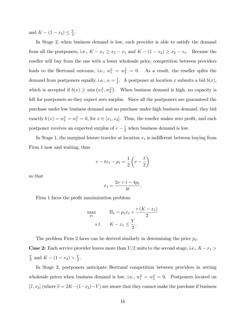
Case 1: Each provider leaves at most 2 units to the second stage, i.e., − 1 ≤ 2and

− (1− 2) ≤ 2

In Stage 2, if business demand is low, each service provider is able to satisfy the demand

for all the postponers, i.e., − 1 ≥ 2 − 1 and − (1 − 2) ≥ 2 − 1. Because the

reseller buys from the provider with the lower wholesale price, competition between providers

leads to the Bertrand outcome, 1 =

2 = 0. As a result, the reseller splits the demand

between the providers equally, i.e., = 12. By (1), the expected surplus of any postponer

from purchasing is − 2− so that the reseller sets retail price = −

2. If business

demand is high, postponers are unable to obtain the service and thus, receive zero surplus.

Therefore, postponers anticipate zero surplus from waiting irrespective of the realization of

business demand. Since the leisure traveler at location is indifferent between purchasing

from Firm in Stage 1 and waiting, we have

− 1 − 1 = 0

1 = − 1

Let Π denote Firm ’s profit, = 1 2. Firm 1 faces the profit maximization problem:

max1

Π1 = 11 + ( − 1)

2

− 1 ≤

2

11

Firm 2 faces a similar problem in deciding 2. The equilibrium solution is presented in

Proposition 1.

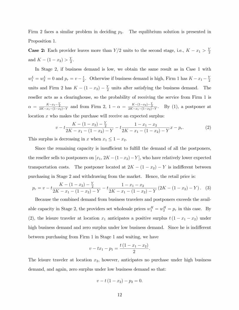
Case 2: Each provider leaves more than 2 units to the second stage, i.e., − 1 2

and − (1− 2) 2

In Stage 2, if business demand is low, we obtain the same result as in Case 1 with

1 =

2 = 0 and = − 2. Otherwise if business demand is high, Firm 1 has −1−

2

units and Firm 2 has − (1− 2) − 2units after satisfying the business demand. The

reseller acts as a clearinghouse, so the probability of receiving the service from Firm 1 is

=−1−

2

2−1−(1−2)− and from Firm 2, 1 − =−(1−2)−

2

2−1−(1−2)− . By (1), a postponer at

location who makes the purchase will receive an expected surplus:

− − (1− 2)−

2

2 − 1 − (1− 2)− −

1− 1 − 2

2 − 1 − (1− 2)− − (2)

This surplus is decreasing in when 1 ≤ 1− 2.

Since the remaining capacity is insufficient to fulfill the demand of all the postponers,

the reseller sells to postponers on [1, 2− (1−2)− ], who have relatively lower expectedtransportation costs. The postponer located at 2 − (1 − 2) − is indifferent between

purchasing in Stage 2 and withdrawing from the market. Hence, the retail price is:

= − − (1− 2)−

2

2 − 1 − (1− 2)− −

1− 1 − 2

2 − 1 − (1− 2)− (2 − (1− 2)− ) (3)

Because the combined demand from business travelers and postponers exceeds the avail-

able capacity in Stage 2, the providers set wholesale prices 1 =

2 = in this case. By

(2), the leisure traveler at location 1 anticipates a positive surplus (1− 1 − 2) under

high business demand and zero surplus under low business demand. Since he is indifferent

between purchasing from Firm 1 in Stage 1 and waiting, we have

− 1 − 1 = (1− 1 − 2)

2

The leisure traveler at location 2, however, anticipates no purchase under high business

demand, and again, zero surplus under low business demand so that:

− (1− 2)− 2 = 0

12

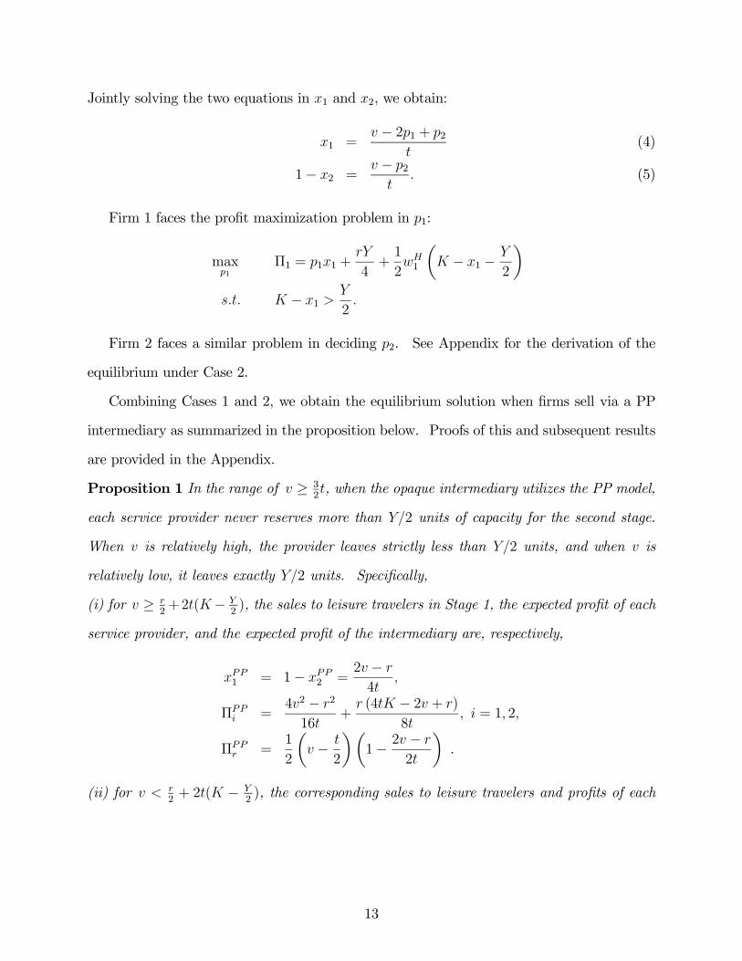
Jointly solving the two equations in 1 and 2, we obtain:

1 = − 21 + 2

(4)

1− 2 = − 2

(5)

Firm 1 faces the profit maximization problem in 1:

max1

Π1 = 11 +

4+1

21

µ − 1 −

2

¶ − 1

2

Firm 2 faces a similar problem in deciding 2. See Appendix for the derivation of the

equilibrium under Case 2.

Combining Cases 1 and 2, we obtain the equilibrium solution when firms sell via a PP

intermediary as summarized in the proposition below. Proofs of this and subsequent results

are provided in the Appendix.

Proposition 1 In the range of ≥ 32, when the opaque intermediary utilizes the PP model,

each service provider never reserves more than 2 units of capacity for the second stage.

When is relatively high, the provider leaves strictly less than 2 units, and when is

relatively low, it leaves exactly 2 units. Specifically,

(i) for ≥ 2+2(−

2), the sales to leisure travelers in Stage 1, the expected profit of each

service provider, and the expected profit of the intermediary are, respectively,

1 = 1− 2 =2 −

4

Π =

42 − 2

16+

(4 − 2 + )

8 = 1 2

Π =

1

2

µ −

2

¶µ1− 2 −

2

¶.

(ii) for 2+ 2( −

2), the corresponding sales to leisure travelers and profits of each

13

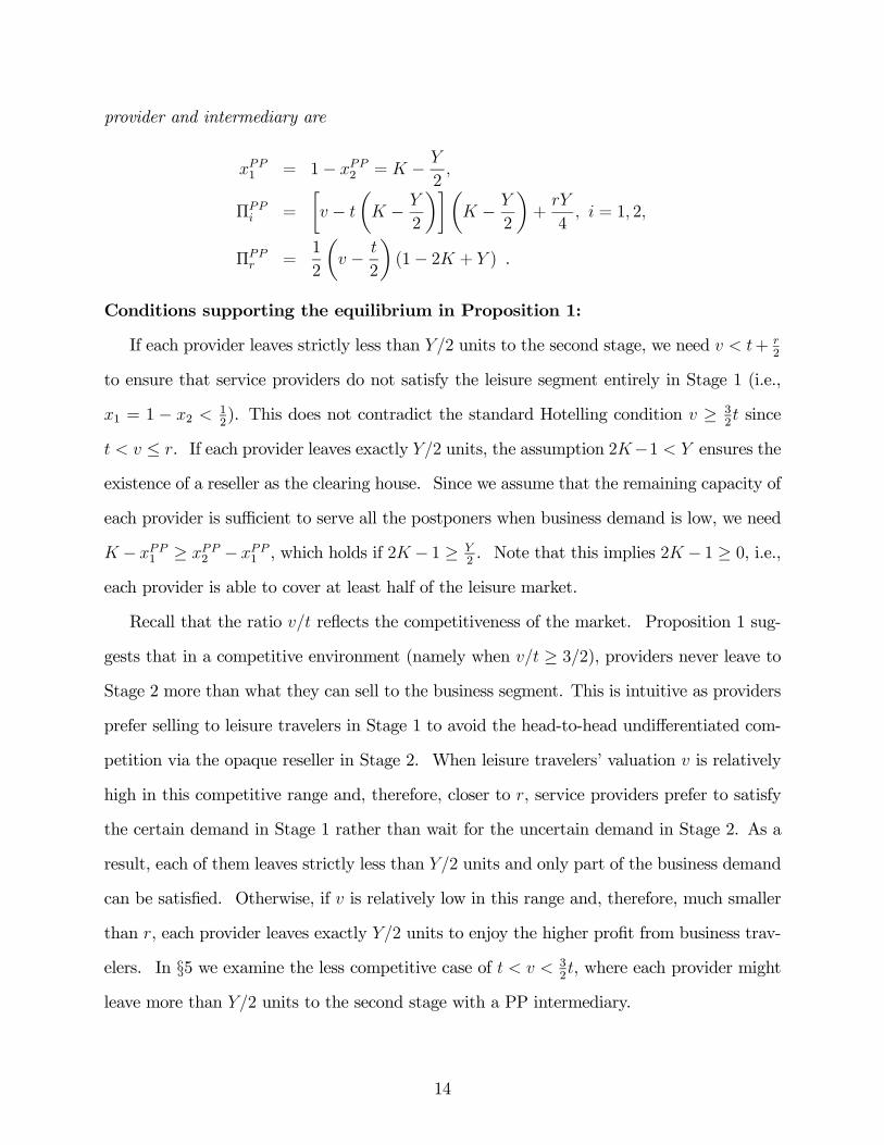
provider and intermediary are

1 = 1− 2 = −

2

Π =

∙ −

µ −

2

¶¸µ −

2

¶+

4 = 1 2

Π =

1

2

µ −

2

¶(1− 2 + ) .

Conditions supporting the equilibrium in Proposition 1:

If each provider leaves strictly less than 2 units to the second stage, we need + 2

to ensure that service providers do not satisfy the leisure segment entirely in Stage 1 (i.e.,

1 = 1 − 2 12). This does not contradict the standard Hotelling condition ≥ 3

2 since

≤ . If each provider leaves exactly 2 units, the assumption 2−1 ensures the

existence of a reseller as the clearing house. Since we assume that the remaining capacity of

each provider is sufficient to serve all the postponers when business demand is low, we need

− 1 ≥ 2 − 1 , which holds if 2 − 1 ≥ 2. Note that this implies 2 − 1 ≥ 0, i.e.,

each provider is able to cover at least half of the leisure market.

Recall that the ratio reflects the competitiveness of the market. Proposition 1 sug-

gests that in a competitive environment (namely when ≥ 32), providers never leave toStage 2 more than what they can sell to the business segment. This is intuitive as providers

prefer selling to leisure travelers in Stage 1 to avoid the head-to-head undifferentiated com-

petition via the opaque reseller in Stage 2. When leisure travelers’ valuation is relatively

high in this competitive range and, therefore, closer to , service providers prefer to satisfy

the certain demand in Stage 1 rather than wait for the uncertain demand in Stage 2. As a

result, each of them leaves strictly less than 2 units and only part of the business demand

can be satisfied. Otherwise, if is relatively low in this range and, therefore, much smaller

than , each provider leaves exactly 2 units to enjoy the higher profit from business trav-

elers. In §5 we examine the less competitive case of 32, where each provider might

leave more than 2 units to the second stage with a PP intermediary.

14

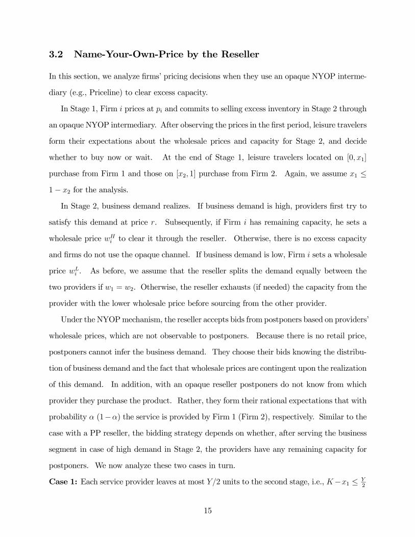
3.2 Name-Your-Own-Price by the Reseller

In this section, we analyze firms’ pricing decisions when they use an opaque NYOP interme-

diary (e.g., Priceline) to clear excess capacity.

In Stage 1, Firm prices at and commits to selling excess inventory in Stage 2 through

an opaque NYOP intermediary. After observing the prices in the first period, leisure travelers

form their expectations about the wholesale prices and capacity for Stage 2, and decide

whether to buy now or wait. At the end of Stage 1, leisure travelers located on [0 1]

purchase from Firm 1 and those on [2 1] purchase from Firm 2. Again, we assume 1 ≤1− 2 for the analysis.

In Stage 2, business demand realizes. If business demand is high, providers first try to

satisfy this demand at price . Subsequently, if Firm has remaining capacity, he sets a

wholesale price to clear it through the reseller. Otherwise, there is no excess capacity

and firms do not use the opaque channel. If business demand is low, Firm sets a wholesale

price . As before, we assume that the reseller splits the demand equally between the

two providers if 1 = 2. Otherwise, the reseller exhausts (if needed) the capacity from the

provider with the lower wholesale price before sourcing from the other provider.

Under the NYOPmechanism, the reseller accepts bids from postponers based on providers’

wholesale prices, which are not observable to postponers. Because there is no retail price,

postponers cannot infer the business demand. They choose their bids knowing the distribu-

tion of business demand and the fact that wholesale prices are contingent upon the realization

of this demand. In addition, with an opaque reseller postponers do not know from which

provider they purchase the product. Rather, they form their rational expectations that with

probability (1−) the service is provided by Firm 1 (Firm 2), respectively. Similar to the

case with a PP reseller, the bidding strategy depends on whether, after serving the business

segment in case of high demand in Stage 2, the providers have any remaining capacity for

postponers. We now analyze these two cases in turn.

Case 1: Each service provider leaves at most 2 units to the second stage, i.e., −1 ≤ 2

15

and − (1− 2) ≤ 2

In Stage 2, when business demand is low, each provider is able to satisfy the demand

from all the postponers, i.e., − 1 ≥ 2 − 1 and − (1 − 2) ≥ 2 − 1. Because the

reseller will buy from the one with a lower wholesale price, competition between providers

leads to the Bertrand outcome, i.e., 1 =

2 = 0. As a result, the reseller splits the

demand from postponers equally, i.e., = 12. A postponer at location submits a bid (),

which is accepted if () ≥ min ¡1

2

¢. When business demand is high, no capacity is

left for postponers so they expect zero surplus. Since all the postponers are guaranteed the

purchase under low business demand and no purchase under high business demand, they bid

exactly () = 2 =

1 = 0, for ∈ [1 2]. Thus, the reseller makes zero profit, and eachpostponer receives an expected surplus of −

2when business demand is low.

In Stage 1, the marginal leisure traveler at location 1 is indifferent between buying from

Firm 1 now and waiting, thus

− 1 − 1 =1

2

µ −

2

¶so that

1 =2 + − 41

4

Firm 1 faces the profit maximization problem:

max1

Π1 = 11 + ( − 1)

2

− 1 ≤

2

The problem Firm 2 faces can be derived similarly in determining the price 2.

Case 2: Each service provider leaves more than 2 units to the second stage, i.e., −1 2and − (1− 2)

2

In Stage 2, postponers anticipate Bertrand competition between providers in setting

wholesale prices when business demand is low, i.e., 1 =

2 = 0. Postponers located on

[b 2] (where b = 2−(1−2)− ) are aware that they cannot make the purchase if business16

demand is high, as they anticipate higher transportation costs compared to those located on

[1 b] given that 1 ≤ 1− 2 from Stage 1. Therefore, those in the range [b 2] choose tobid zero, so that they are guaranteed the service only if business demand is low. Postponers

located on [1 b] place a bid to be granted the service even in case of high business demand.The postponer at location b is indifferent between bidding zero (to win the ticket under lowbusiness demand only) and b (to win the ticket always). This reasoning allows us to derivethe value of b. Postponers on [1 b] bid b by anticipating the service providers’ decision1 =

2 =b when business demand is high. Thus, the reseller makes positive profits only

when business demand is low, taking advantage of the segment of postponers who submit

positive bid b, while paying zero wholesale prices at 1 =

2 = 0. We then back solve

for the providers’ equilibrium in Stage 1. The details of the derivation can be found in the

Appendix.

Proposition 2 shows that with a NYOP reseller, each provider might leave more than

2 units for the second stage under the standard Hoteling condition, i.e., ≥ 32. This is

in contrast with the result under the PP mechanism, where firms never reserve for Stage 2

more than what they can sell to the business segment.

Proposition 2 In the range of ≥ 32, when the opaque intermediary utilizes the NYOP

model, the service providers’ strategy depends on their capacity.

(i) When capacity is quite large with 2 − 79and 9 − 9

2− 2, each provider

reserves at least 2 units for the second stage and there exist multiple equilibria for first

stage pricing, with

1 = 1−

2 ∈∙ − (2 − 2− )

7 −

2

¸

Π =

µ −

1 − 12

µ −

2

¶¶ 1 +

4+1

4

µ −

2

¶µ −

1 −

2

¶

= 1 2. The expected profit of the intermediary is

Π =

1

2

µ −

2

¶µ −

1 −

2

¶.

17

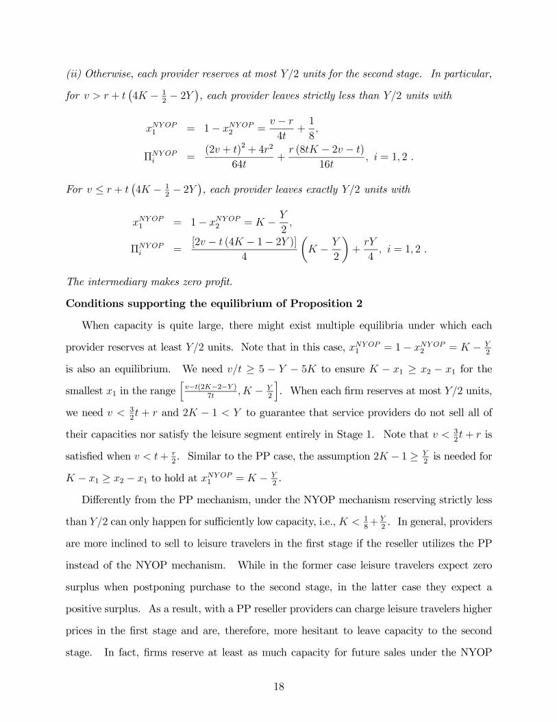
(ii) Otherwise, each provider reserves at most 2 units for the second stage. In particular,

for + ¡4 − 1

2− 2 ¢, each provider leaves strictly less than 2 units with

1 = 1−

2 = −

4+1

8

Π =

(2 + )2+ 42

64+

(8 − 2 − )

16 = 1 2 .

For ≤ + ¡4 − 1

2− 2 ¢, each provider leaves exactly 2 units with

1 = 1−

2 = −

2

Π =

[2 − (4 − 1− 2 )]4

µ −

2

¶+

4 = 1 2 .

The intermediary makes zero profit.

Conditions supporting the equilibrium of Proposition 2

When capacity is quite large, there might exist multiple equilibria under which each

provider reserves at least 2 units. Note that in this case, 1 = 1−

2 = − 2

is also an equilibrium. We need ≥ 5 − − 5 to ensure − 1 ≥ 2 − 1 for the

smallest 1 in the rangeh−(2−2− )

7 −

2

i. When each firm reserves at most 2 units,

we need 32 + and 2 − 1 to guarantee that service providers do not sell all of

their capacities nor satisfy the leisure segment entirely in Stage 1. Note that 32+ is

satisfied when + 2. Similar to the PP case, the assumption 2 − 1 ≥

2is needed for

− 1 ≥ 2 − 1 to hold at 1 = −

2.

Differently from the PP mechanism, under the NYOP mechanism reserving strictly less

than 2 can only happen for sufficiently low capacity, i.e., 18+

2. In general, providers

are more inclined to sell to leisure travelers in the first stage if the reseller utilizes the PP

instead of the NYOP mechanism. While in the former case leisure travelers expect zero

surplus when postponing purchase to the second stage, in the latter case they expect a

positive surplus. As a result, with a PP reseller providers can charge leisure travelers higher

prices in the first stage and are, therefore, more hesitant to leave capacity to the second

stage. In fact, firms reserve at least as much capacity for future sales under the NYOP

18

mechanism as they do under the PP mechanism. In particular, when capacity is relatively

large, i.e., ≥ 718+

2, each provider reserves more than 2 units when the valuation is

below a certain threshold, so that some capacity remains available for postponers even when

business demand is high.

Conventional wisdom suggests that service providers reserve capacity only for customers

with a higher willingness to pay (e.g., business travelers). However, a relative large capacity

depresses the prices that providers can set in the first stage. In addition, providers with a

NYOP reseller make positive profits from selling to postponers. As a result, each provider

may leave more than 2 units for future sales when clearing excess capacity via a NYOP

reseller.

3.3 Direct Selling

In this section, we consider the case when service providers directly sell to customers without

using an intermediary. In the absence of a reseller, postponers can identify the seller and

choose their preferred provider. If business demand is low, postponers can be served as

last minute travelers. On the other hand, if business demand is high, service providers can

no longer price discriminate and must offer the same price to both business travelers and

postponers. As before, there are two cases, which we consider in turn.

Case 1: Each provider leaves at most 2 units to the second stage, i.e., − 1 ≤ 2and

− (1− 2) ≤ 2

In Stage 2, if business demand realization is low, the service providers compete à là

Hotelling for postponers on segment [1 2]. Therefore, 1 and

2 are charged directly to

postponers. Let e denote the location of the postponer who is indifferent between buyingfrom Firm 1 and Firm 2. Thus,

e = 1

2+

2 −

1

2

Firm 1 and 2’s profit in the second stage are 1 (e− 1) and

2 (2 − e), respectively.19

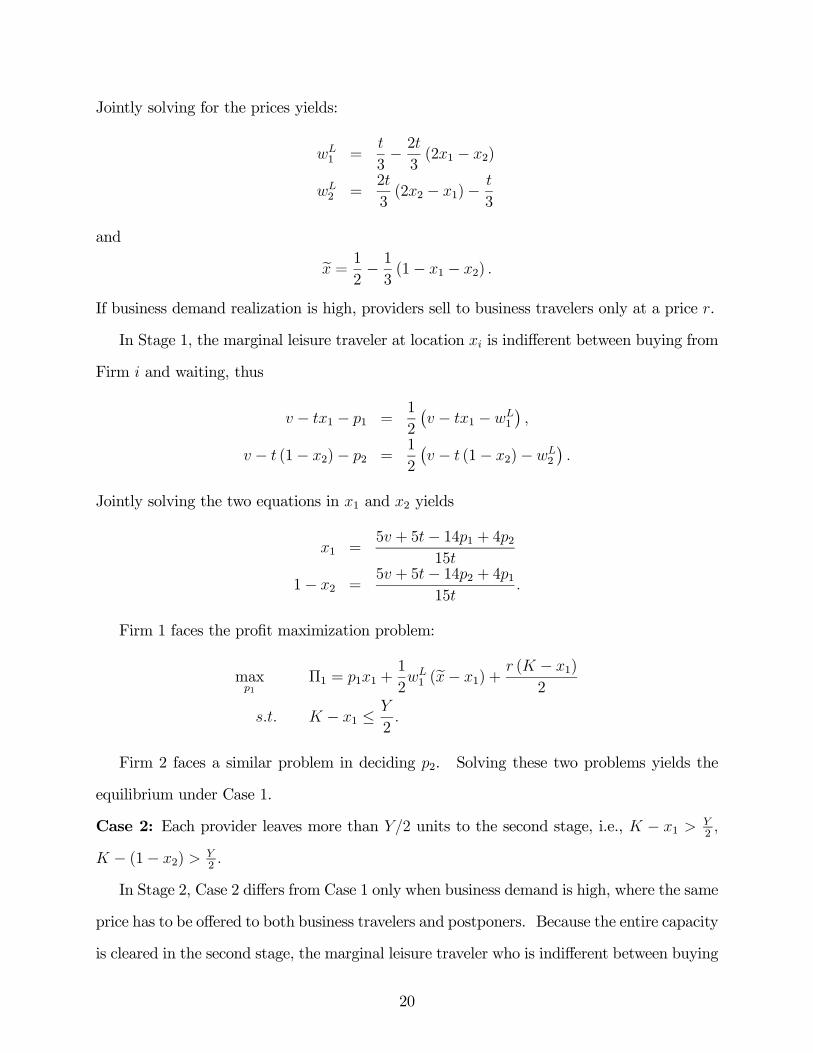
Jointly solving for the prices yields:

1 =

3− 23(21 − 2)

2 =

2

3(22 − 1)−

3

and

e = 1

2− 13(1− 1 − 2)

If business demand realization is high, providers sell to business travelers only at a price .

In Stage 1, the marginal leisure traveler at location is indifferent between buying from

Firm and waiting, thus

− 1 − 1 =1

2

¡ − 1 −

1

¢

− (1− 2)− 2 =1

2

¡ − (1− 2)−

2

¢

Jointly solving the two equations in 1 and 2 yields

1 =5 + 5− 141 + 42

15

1− 2 =5 + 5− 142 + 41

15

Firm 1 faces the profit maximization problem:

max1

Π1 = 11 +1

21 (e− 1) +

( − 1)

2

− 1 ≤

2

Firm 2 faces a similar problem in deciding 2. Solving these two problems yields the

equilibrium under Case 1.

Case 2: Each provider leaves more than 2 units to the second stage, i.e., − 1 2

− (1− 2) 2

In Stage 2, Case 2 differs from Case 1 only when business demand is high, where the same

price has to be offered to both business travelers and postponers. Because the entire capacity

is cleared in the second stage, the marginal leisure traveler who is indifferent between buying

20

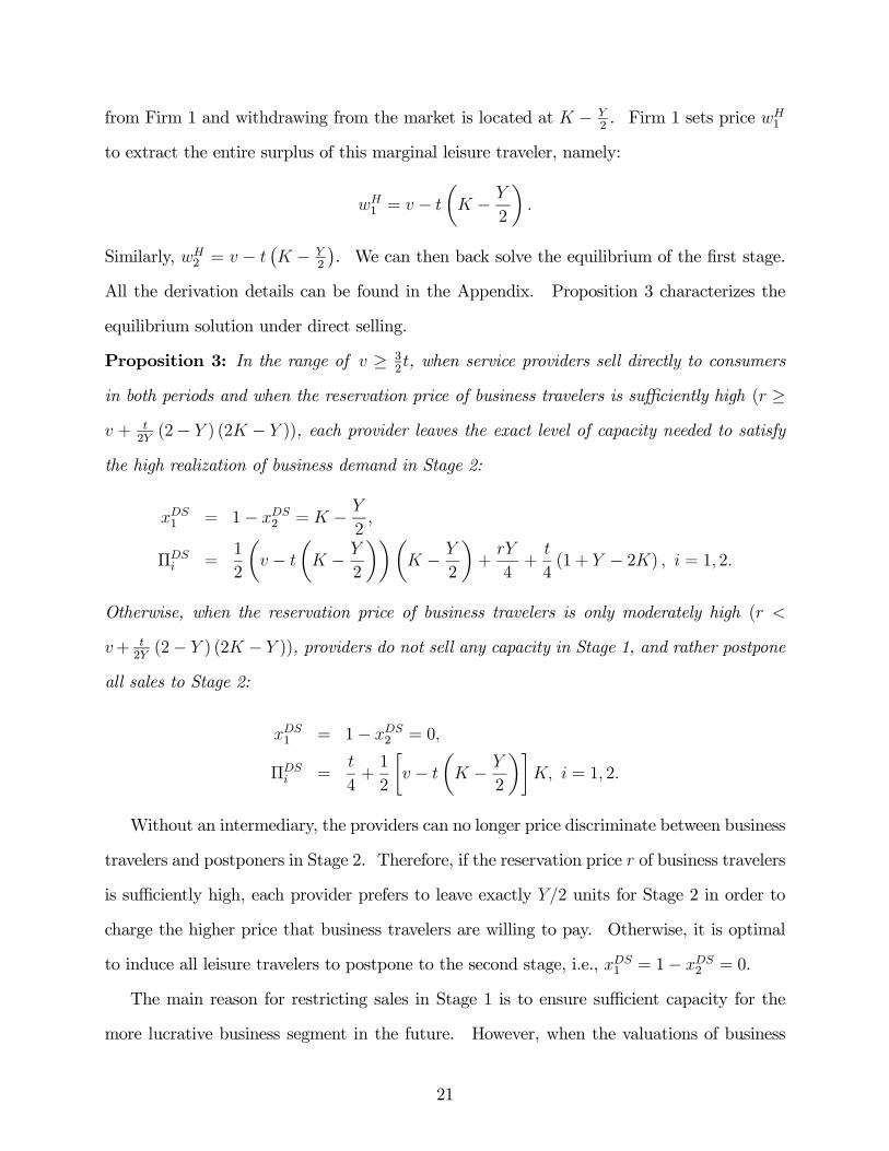
from Firm 1 and withdrawing from the market is located at − 2. Firm 1 sets price

1

to extract the entire surplus of this marginal leisure traveler, namely:

1 = −

µ −

2

¶

Similarly, 2 = −

¡ −

2

¢. We can then back solve the equilibrium of the first stage.

All the derivation details can be found in the Appendix. Proposition 3 characterizes the

equilibrium solution under direct selling.

Proposition 3: In the range of ≥ 32, when service providers sell directly to consumers

in both periods and when the reservation price of business travelers is sufficiently high ( ≥ +

2(2− ) (2 − )), each provider leaves the exact level of capacity needed to satisfy

the high realization of business demand in Stage 2:

1 = 1−

2 = −

2

Π =

1

2

µ −

µ −

2

¶¶µ −

2

¶+

4+

4(1 + − 2) = 1 2

Otherwise, when the reservation price of business travelers is only moderately high (

+ 2(2− ) (2 − )), providers do not sell any capacity in Stage 1, and rather postpone

all sales to Stage 2:

1 = 1−

2 = 0

Π =

4+1

2

∙ −

µ −

2

¶¸ = 1 2

Without an intermediary, the providers can no longer price discriminate between business

travelers and postponers in Stage 2. Therefore, if the reservation price of business travelers

is sufficiently high, each provider prefers to leave exactly 2 units for Stage 2 in order to

charge the higher price that business travelers are willing to pay. Otherwise, it is optimal

to induce all leisure travelers to postpone to the second stage, i.e., 1 = 1−

2 = 0.

The main reason for restricting sales in Stage 1 is to ensure sufficient capacity for the

more lucrative business segment in the future. However, when the valuations of business

21

and leisure travelers are comparable, service providers prefer to sell everything after the

uncertainty is resolved. Interestingly, for sufficiently large business segment ( ≥ 2), it isnever optimal to leave the entire capacity to Stage 2. Instead, each provider reserves exactly

2 units for this stage. For such a large segment of business travelers, the providers are not

willing to give up the opportunity to charge the higher price . If all sales are postponed to

the second stage, providers can no longer discriminate between leisure and business travelers

and have to charge a price lower than to clear the capacity. Another interesting point is

that in contrast to the result derived when a reseller is present, it is never optimal to leave

strictly less than 2 units to the second stage. This implies that the business segment

is always fully served when the providers sell directly to consumers, which need not be

the case with an opaque intermediary. Furthermore, providers can earn positive profits

from the leisure segment in Stage 2 even when business demand is low due to the observable

differentiation between them. In contrast, opacity removes differentiation between providers

and intensifies competition, leading to the Bertrand outcome of zero profits when business

demand is low.

4 Comparison of PP, NYOP and Direct Selling

In this section, we first compare the two opaque selling mechanisms (PP and NYOP) in

terms of profits for competing service providers. We also compare them with direct selling

to better understand the advantages and disadvantages of using an opaque intermediary.

While postponers expect positive surplus in Stage 2 under NYOP, under PP they receive

zero surplus if they wait. As a result, the prices in Stage 1 are higher under PP than

under NYOP, and firms with a NYOP reseller prefer leaving at least as much capacity for

future sales as they do with a PP reseller. For instance, when is moderately high, i.e.,

2+ (2 − ) +

¡4 − 1

2− 2 ¢, each provider reserves exactly 2 units to

the second stage under NYOP, but leaves strictly less than 2 units and receives a lower

Stage 2 profit under PP. In spite of that, the higher profits that accrue in Stage 1 under

22

PP compensate for the loss in Stage 2. Our next proposition states that if service providers

use one opaque intermediary to clear excess capacity, they prefer that the reseller utilizes

the PP rather than the NYOP mechanism.

Proposition 4: If service providers use an opaque intermediary in the second stage, they

prefer the reseller to utilize the PP rather than the NYOP mechanism.

The strict dominance of PP over NYOP can be explained by the different roles the reseller

plays in the two mechanisms. While under NYOP, the reseller is a passive agent who simply

accepts or rejects bids based on wholesale prices, under PP he sets a price to postponers

and can, therefore, more successfully extract their surplus. In fact, when ≥ 32, the

PP reseller extracts the entire expected surplus of postponers. On the other hand, under

NYOP, postponers can retain a positive surplus by anticipating that with some probability

significant excess capacity may materialize, in which case they will gain access to the service

even with a very low bid of zero. Such expectations on the part of postponers force the

providers to set lower prices in their direct channels in Stage 1, thus diminishing the potential

benefit from intertemporal price discrimination. As a result, service providers always make

higher profits by selling via a PP reseller. In §5 we show that this result continues to hold

in a less competitive environment or when capacity is tighter.

The comparison of the PP and NYOP mechanisms with competing providers contrasts

with the findings in Gal-Or (2009), which shows that NYOP is preferable to PP for a

monopoly service provider. The main reason for the different result is the role the opaque

PP reseller plays as a common agent serving both providers. In this role, he can more

successfully extract the surplus of the postponers, which facilitates the providers to set higher

prices in Stage 1. Gal-Or (2009) considers a monopoly service provider who faces travelers

with vertically differentiated valuations for the product. In this case, NYOP allows for more

effective price discrimination among customers than PP and results in a higher profit. Our

result suggests that for routes with fierce competition (e.g., flights between New York and

Chicago), service providers should consider using a PP reseller, whereas for routes with a

23

monopoly provider (e.g., flights between Ithaca, NY and Pittsburgh, PA), clearing excess

capacity through a NYOP reseller is more appropriate.

The comparison of the two pricing mechanisms from the perspective of the intermediary

is ambiguous. When each provider reserves at most 2 units to the second stage, the

opaque intermediary makes zero profit under the NYOP mechanism and thus, prefers the

PP mechanism. However, with larger capacity and low valuation of the leisure segment,

each provider chooses to leave more than 2 units under NYOP so that the intermediary

makes positive profits in this case. Depending on the equilibrium chosen by the providers, a

large segment of leisure travelers may postpone to bid in the second stage, which sometimes

avails a higher profit to the intermediary under NYOP.

From the perspective of service providers, the NYOP mechanism is dominated by the

PP mechanism. Thus, we are interested in comparing direct selling with the PP mechanism

only, as shown in the proposition below.

Proposition 5: The comparison of direct sales with a PP reseller is ambiguous:

(i) If each service provider chooses to leave all the capacity to the second stage under direct

selling, then selling via one opaque PP reseller is always preferable.

(ii) If each service provider chooses to reserve exactly 2 units to the second stage under

direct selling, then having one PP opaque reseller is beneficial when v is sufficiently high.

Proposition 5 suggests that contracting with an intermediary who utilizes a PP mecha-

nism may or may not result in higher profits to service providers. In comparison to direct

selling, opaque selling removes differentiation between providers and intensifies price com-

petition in the second stage, which leads to zero wholesale prices when business demand is

low. As a result, the opaque PP reseller, rather than the providers, earns positive profit

from selling to postponers in Stage 2.

Despite the disadvantage above, there are some benefits of using an agent in the clearance

market. First, the opaque PP reseller improves intertemporal price discrimination among

leisure travelers in comparison to what providers are able to accomplish on their own. As a

24

common agent, a single reseller coordinates the retail price and extracts the entire expected

surplus from postponers, which allows the providers to charge a higher price in the first

stage. Second, an opaque reseller provides an effective way of clearing excess capacity under

stochastic demand (Gal-Or 2009). Acting as a separate clearinghouse, the reseller allows the

providers to sell at a premium price to business travelers while charging a different price to

postponers, thus facilitating price discrimination between business travelers and postponers.

By contrast, a common price has to be offered to both segments of consumers in the absence

of a reseller.4

If the valuation of business travelers is low, providers who sell directly to consumers

prefer selling every unit in the second stage after business demand is realized. In this case,

having an opaque reseller is always beneficial, because it helps clear excess capacity under

uncertain demand while facilitating price discrimination between postponers and business

travelers. However, if is high, each provider reserves exactly 2 units to the second stage

when no intermediary is involved. In this case, direct selling is preferable if the valuation

of leisure travelers is sufficiently low. Recall that the existence of a PP reseller implies

that providers cannot derive any profits from postponers, but can raise prices charged from

leisure travelers in the first stage due to the coordinating role played by the common reseller.

When the reservation price of leisure travelers is sufficiently high, the benefit from higher

prices in the first stage is significant and more than outweighs the loss from the absence

of profits from postponers in the second stage. Note that with direct selling, the providers

derive positive profits from postponers in the second stage due to the absence of opacity.

Hence, when is sufficiently high, providers prefer the PP reseller over direct selling and

when is sufficiently low the opposite result holds.

The result reported in Proposition 5 might appear contradictory to that derived in Jerath

et al. (2010). They demonstrate that direct selling dominates selling via an opaque PP

4Later in §5, we show that it can be optimal to leave more than 2 units under both PP and NYOP

in the range 32. In that case, as well, the opaque reseller facilitates price discrimination between

business travelers and postponers.

25

reseller when is very high. However, they obtain this result for the case where providers

find it optimal not to reserve any capacity for the second stage. In the context of our model,

this would imply that + 2, under which the opaque reseller is no longer active. In

our study, we restrict our derivation to + 2. Proposition 5 reports that direct

selling dominates for the lower portion of this region of values, and the PP mechanism

dominates for the upper portion of this region. In Jerath et al., PP dominates direct selling

throughout the region of values that induce the providers to reserve capacity for the opaque

channel. The main reason for the different results obtained here is that, unlike in Jerath et

al., in our setting, providers do not decide collusively with the intermediary on how to divide

the surplus that accrues in the opaque channel according to a predetermined percentage.

Instead, providers non-cooperatively set wholesale prices for the intermediary, leading to

fierce competition and zero profits to the providers in the second stage when business demand

is low. Hence, the benefit from transacting with the reseller is more moderate in our setting

than in Jerath et al., and if is sufficiently low, direct selling dominates.

We also verify that competing providers prefer direct selling over sales via an opaque

NYOP reseller if under NYOP each provider reserves at most 2 units. Nevertheless,

direct sales can be inferior if each provider leaves more than 2 units to the second stage.

5 Extensions

In this section, we consider three extensions of our model. In the interest of length, we only

present the major results while the derivations can be found in the Appendix.

5.1 Less Competitive Environment 32

Our base model assumes ≥ 32. In the standard Hotelling model, this condition avails a

competitive environment so that the entire Hotelling line is served. We now consider a less

competitive environment with 32. The equilibrium derivation is similar to that in

the base model (see Appendix for details). The proposition below summarizes the results.

26

Proposition 6: When 32,

(i) service providers who sell via a PP reseller may reserve more than 2 units for the

second stage when capacity is relatively large. In this case, there exist multiple equilibria in

setting first stage prices, among which reserving exactly 2 units yields the lowest profit.

(ii) competing providers still prefer the PP over the NYOP mechanism.

(iii) providers prefer selling directly to consumers over transacting with a PP reseller when

is sufficiently low.

While under ≥ 32service providers with a PP reseller never reserve more than what

they can sell to the business segment, for 32, each provider may reserve more than 2

units under either selling mechanism so that some capacity remains available for postponers

even if business demand is high. When the valuation is low, providers are unable to set

high prices in the first stage, and they no longer engage in fierce competition. As a result,

reserving capacity for leisure travelers who postpone their purchase decisions becomes more

attractive.

The comparison of the PP and the NYOP mechanisms for 32is complicated by

the fact that multiple equilibria may arise under one or both mechanisms. Nevertheless,

comparing the equilibrium that generates the highest profits to the providers under NYOP

with the one that generates the lowest profits under PP, we conclude that the PP mechanism

continues to dominate the NYOP mechanism.

The comparison of the PP mechanism and direct selling may also involve multiple equi-

libria. However, even restricting attention to the equilibrium under PP that generates the

highest profits for the providers, it is still possible for direct selling to outperform selling via

an opaque PP reseller. For a less competitive environment with lower valuation , using

an intermediary as the common agent to alleviate price competition in the first stage is less

essential, so that direct selling becomes more preferable.

27

5.2 Multiple Resellers

In this section we extend our analysis by allowing the presence of multiple opaque interme-

diaries in the market. Specifically, we consider two competing resellers who can use either

PP or NYOP, and each can serve both service providers. This setup is consistent with

the observation that competing resellers, such as Priceline and Hotwire, serve multiple air-

lines and hotels. We consider three possible scenarios: a) both resellers utilize PP, b) both

resellers utilize NYOP, and c) one reseller utilizes PP while the other utilizes NYOP. We

characterize the equilibrium of these scenarios, and compare them with the equilibrium when

a single reseller is used. Due to model tractability, we do not analyze the asymmetric case

where one firm contracts with one reseller, while the other firm contracts with both resellers.

Rather, our study simply compares the profits when the two identical firms follow the same

strategy in clearing excess capacity. The results of this comparison are summarized in the

proposition below.

Proposition 7: Competition among opaque resellers may reduce the benefit derived by ser-

vice providers in comparison to selling via a single intermediary. In particular,

(i) providers prefer selling via a single PP reseller than via two competing PP resellers.

(ii) providers are indifferent between selling via a single NYOP reseller or via multiple com-

peting NYOP resellers.

(iii) for competing providers, selling via two competing PP resellers is equivalent to selling

via one PP and one NYOP reseller, and is equivalent to selling via one or more NYOP

resellers when each provider leaves at most 2 units to second stage.

Proposition 7 states that when competing service providers clear excess capacity through

opaque intermediaries, their profits are the highest when they sell via a single posted price

reseller. Conventional wisdom might suggest that service providers can take advantage

of competition among downstream resellers. However, in the presence of two competing

providers, a single PP reseller is more successful than competing resellers in extracting surplus

from postponers when low business demand realizes. In fact, postponers can retain positive

28

surplus when resellers compete, thus preventing providers from setting high prices in Stage

1. Hence, a single PP reseller is preferable to competing resellers from the perspective

of providers. This result is consistent with those derived in the economics and marketing

literature on common agency (McGuire and Staelin 1983, Bernheim and Whinston 1985,

1986, Choi 1991, Gal-Or 1991), which shows that a single common agent is necessary to

facilitate collusion among competitors.

The analysis of multiple competing NYOP resellers is similar to that with a single NYOP

reseller, due to the passive role of resellers under the bidding model. The only difference

is that the resellers will equally split the positive profits, if any, generated from the NYOP

channel. Nevertheless, the providers earn the same profits under one or multiple NYOP

resellers.

When there are two competing resellers, one using PP and the other using NYOP, post-

poners can infer the state of business demand from the retail price in the PP channel.

Therefore, postponers bid at zero when business demand is low. Due to the competition

with the NYOP reseller, the PP reseller is forced to price at zero as well, leaving surplus to

postponers as in the case with two PP resellers. In fact, providers are indifferent between

selling via two PP resellers and selling via one PP and one NYOP reseller. Therefore, for

competing service providers, contracting with both Hotwire and Priceline is equivalent to

using two Hotwire-type resellers.

Overall, for competing providers, one opaque PP reseller is preferable to other strategies

that involve one or two intermediaries. Thus, if for a certain route competing airlines have

already contracted with Hotwire, jointly adding Priceline or any other opaque reseller to the

distribution channel may reduce profits.

5.3 Mixed Strategy Equilibria

So far, we assume that each provider has enough capacity to fulfill the postponers’ demand

when business demand is low, i.e., − 1 ≥ 2 − 1 and − (1 − 2) ≥ 2 − 1. This

29

assumption ensures a pure strategy equilibrium for the price competition in the second stage.

We now turn to the case where each provider is unable to fulfill the postponers’ demand,

however the total capacity is sufficient to cover the leisure segment, i.e., 2 − 1 ≥ 0.5

In the interest of length, we consider a representative case where each provider leaves at

most 2 units to the second stage. The equilibrium derivation can be found in the Ap-

pendix. With a posted price reseller, the tighter capacity leads to mixed strategy equilibria

when business demand is low and thus, providers obtain positive profits in Stage 2. The

retail price still extracts the entire surplus from postponers, but the reseller now shares this

surplus with providers because wholesale prices are no longer zero when firms adopt a mixed

strategy. The process of setting prices in the first stage is similar to that under the pure

strategy. Overall, providers enjoy higher profits when capacity declines. However, because

the total capacity is still sufficient to cover the entire leisure market when business demand

is low, the results under NYOP and direct selling are similar to those derived in the base

case. Therefore, the PP mechanism continues to dominate the NYOP mechanism from the

perspective of the providers. Providers are also more likely to favor the PP mechanism over

direct selling, given the higher profits they can expect in the second stage with a PP reseller.

6 Discussion and Conclusion

Opaque retailers, such as Priceline and Hotwire, offer an alternative distribution channel for

service providers in the travel industry. By selling “last minute” special deals whose at-

tributes are hidden before the purchase, these intermediaries allow the providers to maintain

high prices in their direct marketing channels while clearing any remaining capacity via the

opaque channel. In this paper, we compare two commonly used opaque selling mechanisms,

i.e., Posted Price (PP) and Name-Your-Own-Price (NYOP), from the perspective of two

5Under extremely limited capacity, the providers cannot cover the leisure market even when business

demand is low, i.e., 2 − 1 0. As postponers face fairly limited capacity, they raise their bids under theNYOP mechanism and receive a lower expected surplus in Stage 2, which allows the providers to set higher

prices in Stage 1. In this case, if it is optimal to leave at most 2 units to Stage 2 under both mechanisms,

the providers will be indifferent between the PP and the NYOP mechanism.

30

competing service providers.

Our study yields several insights regarding the impact of different selling mechanisms on

the profits of competing service providers. If providers clear excess capacity through a single

opaque intermediary we find that they prefer a reseller who utilizes a posted price mechanism

over one who uses a bidding model. In fact, under NYOP, the reseller is a passive agent who

simply accepts or rejects bids given the wholesale prices set by the providers. In contrast,

under PP the reseller sets the retail price and, therefore, can more successfully extract the

surplus of leisure travelers who postpone their purchase decisions. With this lower expected

surplus of postponers, service providers can set higher prices in their own marketing channels

in the advance period. As a result, a PP retailer provides a more effective vehicle than an

NYOP retailer to alleviate price competition among providers. Such alleviated competition

leads, in turn, to higher profits for the providers. This result contrasts with that derived

in the existing literature for a monopoly service provider, whose profit is higher when the

opaque reseller uses the NYOP instead of the PP model.

For comparison purposes, we also consider the possibility that the providers use their

direct channels to dispose of remaining capacity. We find that direct selling of excess capacity

may dominate opaque reselling when the valuation of the leisure segment is low. Recall that

opaque reselling may introduce both advantages and disadvantages to the providers. The

advantages are the higher prices that providers can set in their direct channels in the advance

period as well as their ability to price discriminate between business and leisure customers.

The disadvantage is the elimination of differentiation when offering an opaque product to

postponers, which exerts downward pressure on prices. We find that when the valuation of

leisure travelers is sufficiently low the latter disadvantage more than outweighs the former

advantages. As a result, service providers may prefer direct selling over using an opaque

PP reseller in this case.

This is the first work that compares different selling mechanisms for competing service

providers who clear excess capacity through an opaque intermediary. For model tractabil-

31

ity, we focus on two identical firms choosing the same strategy. It would be interesting to

investigate environments where firms choose different strategies, e.g., one selling through a

PP reseller, while the other through a NYOP reseller. With such asymmetry in the choice of

the pricing model opacity disappears completely. To preserve opacity, it would be necessary

to consider settings with at least three providers. Such an extension can help explain why

some airlines, e.g., Southwest Airlines, choose to serve customers through their direct chan-

nels only, whereas others contract with opaque intermediaries. The full characterization

of multiple firms’ equilibrium strategies in the presence of multiple resellers with different

selling mechanisms is left for future research.

In our model, leisure travelers derive the same intrinsic utility from the service regardless

of whether they purchase it directly from the provider or from an opaque channel. How-

ever, sometimes products sold through an opaque retailer are “damaged” in that some key

information, such as flight departure time, is not disclosed until the purchase is made. In

addition, the refund or cancellation policy is usually stringent for opaque products. This

“damaged” property of opaque goods is likely to make leisure travelers more hesitant to post-

pone their purchase. Future studies can examine how this change in the valuation of opaque

products affects the profitability of direct versus opaque selling through intermediaries.

Service capacity in the travel industry is usually hard to adjust in the short term. Thus,

we model the capacity as exogenous in this paper. However, firms can expand or reduce

their capacity over a longer time horizon. Future research could consider a multi-stage game

in which capacity is endogenously chosen by service providers before they engage in price

competition. Finally, most of the empirical analysis related to opaque selling focuses on

consumers’ bidding strategies. It may be interesting to also empirically test the behavior of

service providers using the theoretical predictions of our paper.

32

References

Beckmann, M. J. 1965. Edgeworth-Bertrand duopoly revisited. In: R. Henn (ed.), Opera-

tions Research-Verfahren, III. Anton Hein Verlag, Meisenheim, Germany, pp. 55-68.

Bernheim, B. D., M. D. Whinston. 1985. Common marketing agency as a device for facili-

tating collusion. RAND Journal of Economics 16(2), 269-281.

Bernheim, B. D., M. D. Whinston. 1986. Common agency. Econometrica 54(4), 923-942.

Bernheim, B. D., M. D. Whinston. 1998. Exclusive dealing. Journal of Political Economy

106(1), 64-103.

Choi, S. C. 1991. Price competition in a channel structure with a common retailer. Marketing

Science 10(4), 271-296.

Choi, S. C. 1996. Price competition in a duopoly common retailer channel. Journal of

Retailing 72(2), 117-134.

Coughlan, A. T. 1985. Competition and cooperation and marketing channel choice: Theory

and application. Marketing Science 4(2), 110-129.

Coughlan, A. T., B. Wernerfelt. 1989. On credible delegation by oligopolists: A discussion

of distribution channel management. Management Science 35(2), 226—239.

Dasgupta, P., E. Maskin. 1986a. The existence of equilibrium in discontinuous economic

games, I: Theory. Review of Economic Studies 53(1), 1-26.

Dasgupta, P., E. Maskin. 1986b. The existence of equilibrium in discontinuous economic

games, II: Theory. Review of Economic Studies 53(1), 27-41.

Edgeworth, F. Y. 1925. The pure theory of monopoly. In: F. Y. Edgeworth (ed.), Papers

related to Political Economy, Vol. 1, Ch. E, Franklyn, New York, NY, pp. 111-142.

Elkind, P. 1999. The hype is big, really big, at Priceline. Fortune, September 6.

Fay, S. 2004. Partial-Repeat-Bidding in the Name-Your-Own-Price channel. Marketing

Science 23(3), 407-418.

Fay, S. 2008. Selling an opaque product through an intermediary: The case of disguising

one’s product. Journal of Retailing 84(1), 59-75.

33

Fay, S. 2009. Competitive reasons for the Name-Your-Own-Price channel. Marketing Letters

20(3), 277-293.

Fay, S., J. Laran. 2009. Implications of expected changes in the seller’s price in Name-Your-

Own-Price auctions. Management Science 55(11), 1783-1796.

Fay, S., J. Xie. 2008. Probabilistic goods: A creative way of selling products and services.

Marketing Science 27(4), 674—690.

Fay, S., J. Xie. 2010. The economics of buyer uncertainty: Advance selling vs. probabilistic

selling. Marketing Science 29(6), 1040-1057.

Gal-Or, E. 1991. A common agency with incomplete information. RAND Journal of Eco-

nomics 22(2), 274-286.

Gal-Or, E. 2009. Pricing practices of resellers in the airline industry: Posted Price vs. Name-

Your-Own-Price models. Journal of Economics and Management Strategy 20(1), 2011.

Garrido, R. 2010. Expedia unpublished rate hotels. Reuters.com. Oct 26.

Hann, I. H., C. Terwiesch. 2003. Measuring the frictional costs of online transactions: The

case of a Name-Your-Own-Price channel. Management Science 49(11), 1563-1579.

Hotelling, H. 1929. Stability in competition. The Economic Journal 39(153), 41—57.

Huang, X., G. Sosic. 2009. Name-Your-Own-Price as a competitive secondary channel in

the presence of posted prices. Working Paper, McGill University, Montreal, Quebec.

Jerath, K., S. Netessine, S. K. Veeraraghavan. 2010. Revenue management with strategic

customers: Last-Minute Selling and Opaque Selling. Management Science 56(3), 430-448.

Jiang, Y. 2007. Price discrimination with opaque products. Journal of Revenue and Pricing

Management 6(2), 118-134.

Levitan, R., M. Shubik. 1972. Price duopoly and capacity constraints. International Eco-

nomic Review 13(1), 111-122.

Martimort, D. 1996. Exclusive dealing, common agency, andmultiprincipals incentive theory.

RAND Journal of Economics 27(1), 1-31.

McGuire, T. W., R. Staelin. 1983. An industry equilibrium analysis of downstream vertical

34

integration. Marketing Science 2(2), 161-191.

Moorthy, K. S. 1988. Strategic decentralization in channels. Marketing Science 7(4), 335-

355.

Osborne, M. J., C. Pitchik. 1986. Price competition in a capacity-constrained duopoly.

Journal of Economic Theory 38(2), 238-260.

Shapiro, D., X. Shi. 2008. Market segmentation: The role of opaque travel agencies. Journal

of Economics and Management Strategy 17(4), 803-837.

Shapiro, D., A. Zillante. 2009. Naming Your Own Price mechanisms: Revenue gain or

drain?. Journal of Economic Behavior and Organization 72(2), 725-737.

Terwiesch, C., S. Savin, I. H. Hann. 2005. Online haggling at a Name-Your-Own-Price

retailer: Theory and application. Management Science 51(3), 339-351.

Turner, S. A. 2010. Expedia expands Hotwire’s opaque rate program. Available at Hotel-

NewsNow.com (retrieved on 17th February 2011).

Wang, T., E. Gal-Or, R. Chatterjee. 2009. The Name-Your-Own-Price channel in the travel

industry: An analytical exploration. Management Science 55(6), 968-979.

Wang, T., M. Y. Hu, A. W. Hao. 2010. Name-Your-Own-Price seller’s information revelation

strategy with the presence of list-price channel. Electronic Markets 20(2), 119—129.

Wilson, J. G., G. Zhang. 2008. Optimal design of a Name-Your-Own-Price channel. Journal

of Revenue and Pricing Management 7(3), 281—290.

35

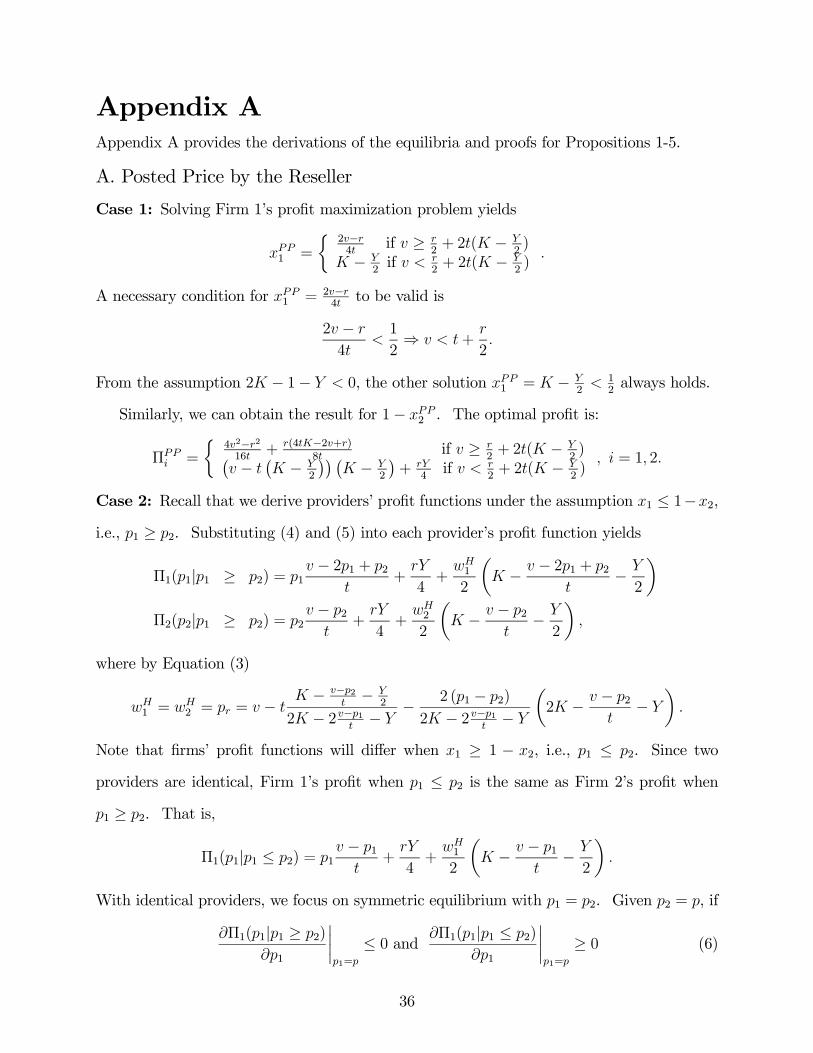
Appendix A

Appendix A provides the derivations of the equilibria and proofs for Propositions 1-5.

A. Posted Price by the Reseller

Case 1: Solving Firm 1’s profit maximization problem yields

1 =

½2−4

if ≥ 2+ 2( −

2)

− 2if

2+ 2( −

2)

A necessary condition for 1 = 2−4

to be valid is

2 −

41

2⇒ +

2

From the assumption 2 − 1− 0, the other solution 1 = − 2 1

2always holds.

Similarly, we can obtain the result for 1− 2 . The optimal profit is:

Π =

½42−216

+(4−2+)

8if ≥

2+ 2( −

2)¡

− ¡ −

2

¢¢ ¡ −

2

¢+

4if

2+ 2( −

2) = 1 2

Case 2: Recall that we derive providers’ profit functions under the assumption 1 ≤ 1−2,

i.e., 1 ≥ 2. Substituting (4) and (5) into each provider’s profit function yields

Π1(1|1 ≥ 2) = 1 − 21 + 2

+

4+

1

2

µ − − 21 + 2

−

2

¶Π2(2|1 ≥ 2) = 2

− 2

+

4+

2

2

µ − − 2

−

2

¶

where by Equation (3)

1 =

2 = = − − −2

−

2

2 − 2−1−

− 2 (1 − 2)

2 − 2−1−

µ2 − − 2

−

¶

Note that firms’ profit functions will differ when 1 ≥ 1 − 2, i.e., 1 ≤ 2. Since two

providers are identical, Firm 1’s profit when 1 ≤ 2 is the same as Firm 2’s profit when

1 ≥ 2. That is,

Π1(1|1 ≤ 2) = 1 − 1

+

4+

1

2

µ − − 1

−

2

¶

With identical providers, we focus on symmetric equilibrium with 1 = 2. Given 2 = , if

Π1(1|1 ≥ 2)

1

¯̄̄̄1=

≤ 0 and Π1(1|1 ≤ 2)

1

¯̄̄̄1=

≥ 0 (6)

36

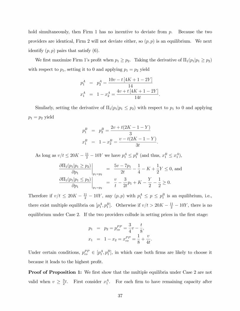
hold simultaneously, then Firm 1 has no incentive to deviate from . Because the two

providers are identical, Firm 2 will not deviate either, so ( ) is an equilibrium. We next

identify ( ) pairs that satisfy (6).

We first maximize Firm 1’s profit when 1 ≥ 2. Taking the derivative of Π1(1|1 ≥ 2)

with respect to 1, setting it to 0 and applying 1 = 2 yield

1 = 2 =10 − [4 + 1− 2 ]

14

1 = 1− 2 =4 + [4 + 1− 2 ]

14

Similarly, setting the derivative of Π1(1|1 ≤ 2) with respect to 1 to 0 and applying

1 = 2 yield

1 = 2 =2 + (2 − 1− )

3

1 = 1− 2 = − (2 − 1− )

3

As long as ≤ 20 − 112− 10 we have 1 ≤ 1 (and thus,

1 ≤ 1 ),

Π1(1|1 ≥ 2)

1

¯̄̄̄1=2

=5 − 712

− 14− +

1

2 ≤ 0, and

Π1(1|1 ≤ 2)

1

¯̄̄̄1=2

=

− 3

21 + −

2− 12≥ 0

Therefore if ≤ 20 − 112− 10 , any ( ) with 1 ≤ ≤ 1 is an equilibrium, i.e.,

there exist multiple equilibria on [1 1 ]. Otherwise if 20 − 11

2− 10 , there is no

equilibrium under Case 2. If the two providers collude in setting prices in the first stage:

1 = 2 = =3

4 −

8

1 = 1− 2 = =1

8+

4

Under certain conditions, ∈ [1 1 ], in which case both firms are likely to choose itbecause it leads to the highest profit.

Proof of Proposition 1: We first show that the multiple equilibria under Case 2 are not

valid when ≥ 32. First consider 1 . For each firm to have remaining capacity after

37

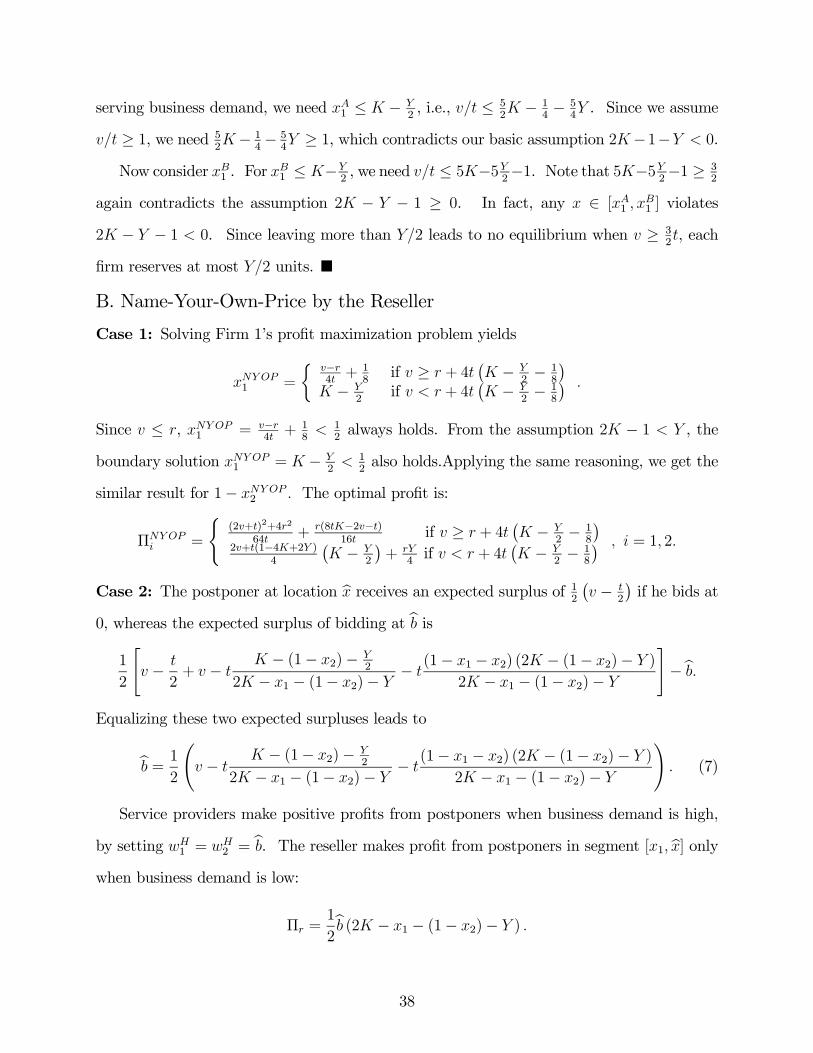
serving business demand, we need 1 ≤ − 2, i.e., ≤ 5

2 − 1

4− 5

4 . Since we assume

≥ 1, we need 52− 1

4− 5

4 ≥ 1, which contradicts our basic assumption 2−1− 0.

Now consider 1 . For 1 ≤ −

2, we need ≤ 5−5

2−1. Note that 5−5

2−1 ≥ 3

2

again contradicts the assumption 2 − − 1 ≥ 0. In fact, any ∈ [1 1 ] violates2 − − 1 0. Since leaving more than 2 leads to no equilibrium when ≥ 3

2, each

firm reserves at most 2 units. ¥

B. Name-Your-Own-Price by the Reseller

Case 1: Solving Firm 1’s profit maximization problem yields

1 =

½−4+ 1

8if ≥ + 4

¡ −

2− 1

8

¢ −

2if + 4

¡ −

2− 1

8

¢

Since ≤ , 1 = −

4+ 1

8 1

2always holds. From the assumption 2 − 1 , the

boundary solution 1 = −

2 1

2also holds.Applying the same reasoning, we get the

similar result for 1− 2 The optimal profit is:

Π =

((2+)2+42

64+

(8−2−)16

if ≥ + 4¡ −

2− 1

8

¢2+(1−4+2 )

4

¡ −

2

¢+

4if + 4

¡ −

2− 1

8

¢ = 1 2

Case 2: The postponer at location b receives an expected surplus of 12

¡ −

2

¢if he bids at

0, whereas the expected surplus of bidding at b is1

2

" −

2+ −

− (1− 2)− 2

2 − 1 − (1− 2)− − (1− 1 − 2) (2 − (1− 2)− )

2 − 1 − (1− 2)−

#−b

Equalizing these two expected surpluses leads to

b = 1

2

à −

− (1− 2)− 2

2 − 1 − (1− 2)− − (1− 1 − 2) (2 − (1− 2)− )

2 − 1 − (1− 2)−

! (7)

Service providers make positive profits from postponers when business demand is high,

by setting 1 =

2 =b. The reseller makes profit from postponers in segment [1 b] only

when business demand is low:

Π =1

2b (2 − 1 − (1− 2)− )

38

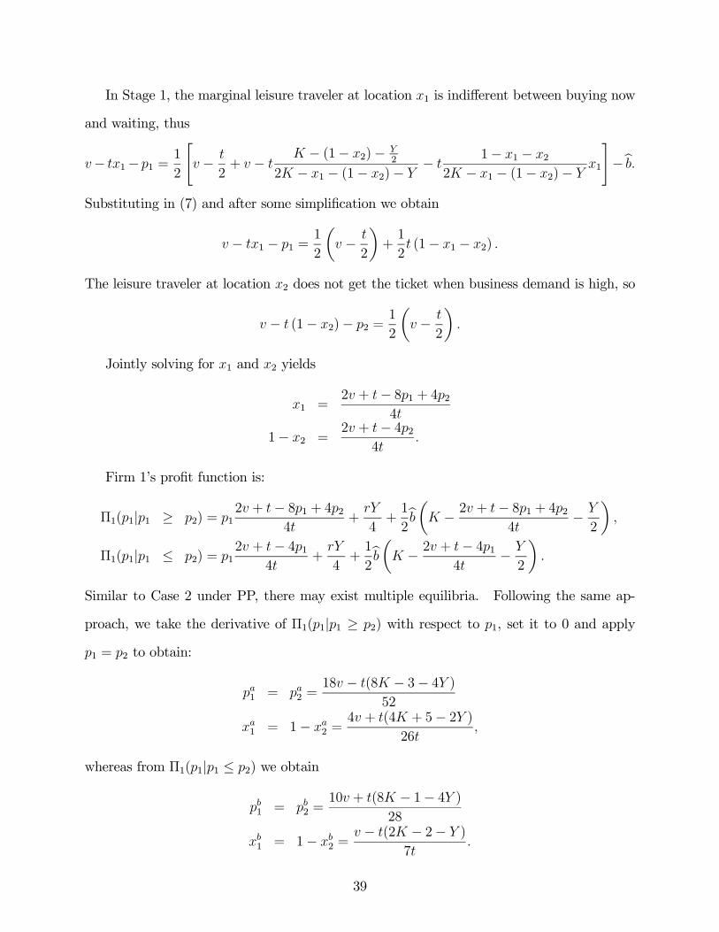
In Stage 1, the marginal leisure traveler at location 1 is indifferent between buying now

and waiting, thus

− 1− 1 =1

2

" −

2+ −

− (1− 2)− 2

2 − 1 − (1− 2)− −

1− 1 − 2

2 − 1 − (1− 2)− 1

#−b

Substituting in (7) and after some simplification we obtain

− 1 − 1 =1

2

µ −

2

¶+1

2 (1− 1 − 2)

The leisure traveler at location 2 does not get the ticket when business demand is high, so

− (1− 2)− 2 =1

2

µ −

2

¶

Jointly solving for 1 and 2 yields

1 =2 + − 81 + 42

4

1− 2 =2 + − 42

4

Firm 1’s profit function is:

Π1(1|1 ≥ 2) = 12 + − 81 + 42

4+

4+1

2bµ − 2 + − 81 + 42

4−

2

¶

Π1(1|1 ≤ 2) = 12 + − 41

4+

4+1

2bµ − 2 + − 41

4−

2

¶

Similar to Case 2 under PP, there may exist multiple equilibria. Following the same ap-

proach, we take the derivative of Π1(1|1 ≥ 2) with respect to 1, set it to 0 and apply

1 = 2 to obtain:

1 = 2 =18 − (8 − 3− 4 )

52

1 = 1− 2 =4 + (4 + 5− 2 )

26

whereas from Π1(1|1 ≤ 2) we obtain

1 = 2 =10 + (8 − 1− 4 )

28

1 = 1− 2 = − (2 − 2− )

7

39

1 ≤ 1 (and thus, 1 ≥ 1) when + (40 − 17

2− 20 ) ≥ 0 so that multiple equilibria

exist on£1

1

¤. If the two providers collude in setting prices in the first stage, then:

1 = 2 = =

16+3

8

1 = 1− 2 = =

3

16+

8

Under certain conditions, ∈ £1 1¤, in which case firms are likely to choose this

equilibrium that yields the highest profit.

Proof of Proposition 2: Under Case 2, 1 ≤ − 2implies ≤ 22−11−5

4. Since we

assume ≥ 32, we need 3

2≤ 22−11−5

4, which contradicts the assumption 2− 1− 0.

Now consider 1 for the constraint 1 ≤ −

2, i.e., ≤ 9 − 9

2− 2. Since ≥ 3

2, this

implies that 2 − ≥ 79 which guarantees + (40 − 17

2− 20 ) ≥ 0, and thus, 1 ≥ 1.

For 1 to be valid, we require under low business demand each firm is able to cover the

entire market of postponers, i.e., − 1 ≥ 2 − 1. This implies ≥ 5− − 5. Notethat

5− − 5 ≤ ≤ 9 − 92− 2⇔ 2 −

2− 1 ≥ 0

which we assume to hold.

Thus, when 2 − ≥ 79and ≤ 9 − 9

2− 2, there exist multiple equilibria with the

corresponding first stage sales 1 = 1−

2 ∈ [−(2−2− )7

−2] and the retailer’sexpected profit isΠ

= 12

¡ −

2

¢ ¡ −

1 − 2

¢. In this case, the boundary solution

of Case 1, 1 = −

2, is also an equilibrium. Otherwise, there is no equilibrium under

Case 2. Thus, we have the interior solution 1 = −

4+ 1

8when ≥ +4

¡ −

2− 1

8

¢and the boundary solution

1 = − 2when + 4

¡ −

2− 1

8

¢. ¥

C. Direct Selling by the Reseller

Case 1: Maximizing Firm 1’s profit in 1 and recalling that at the symmetric equilibrium

1 = 2, we have

1 =21 + 23−

40and 1 =

7 − 7 −

20

40

Note that 7 − 7 − 0 since ≥ Therefore the solution is at the boundary, where

1 =5 + 5− 141 + 42

15= −

2

As we focus on symmetric equilibrium, we have

1 =

+ ¡1− 3 + 3

2

¢2

and 1 = −

2.

The indifferent leisure traveler needs to enjoy a nonnegative utility in the second stage:

−

2− 1 ≥ 0⇔ ≥ 3

2− (2 − )

The profit is

Π =

1

2

µ −

µ −

2

¶¶µ −

2

¶+

4+

4(1 + − 2) = 1 2

Case 2: If each firm leaves more than 2, under low business demand we have

1 =

3− 23(21 − 2)

2 =

2

3(22 − 1)−

3

whereas under high business demand the wholesale prices are

1 =

2 = −

µ −

2

¶

The interior solution (1 ,

2 ) requires ≥ 3

2. If 3

2, the leisure traveler located at

= 12incurs a negative utility with probability 1

2.

Because leisure travelers at location 1 and 2 are indifferent between buying now and

waiting, we have

1 =1

2

µ

3− 23(21 − 2)

¶+1

2

µ −

µ −

2

¶¶2 =

1

2

µ2

3(22 − 1)−

3

¶+1

2

µ −

µ −

2

¶¶

which leads to

1 =2 − (2 − 2− )− 81 + 42

4

1− 2 =2 − (2 − 2− )− 82 + 41

4

41

Firm 1’s profit is Π1 = 11+121 (e− 1)+

121 ( − 1) Taking the derivative in 1

and considering 1 = 2 at the symmetric equilibrium, we get:

1 =

1

2

µ −

µ − 1−

2

¶¶and

1 = 0

Note that in this case,

− 1 − 1 =1

2

¡ − 1 −

1

¢+1

2

¡ − 1 −

1

¢1 =

1

2

£1 +

1

¤ (8)

which holds for any 1 − 2. Since Firm 1 prefers 1 = 0, he can raise 1 slightly so

that every leisure traveler prefers to wait. The same analysis and logic applies to Firm 2.

The optimal profit is

Π =

4+1

2

∙ −

µ −

2

¶¸ = 1 2

Proof of Proposition 3: Comparing the profit under Cases 1 and 2, we know

4+1

2

∙ −

µ −

2

¶¸ ≤ 1

2

µ −

µ −

2

¶¶µ −

2

¶+

4+

4(1 + − 2)

⇔ ≥ +

2(2− ) (2 − )

Thus when is relatively high, each firm reserves exactly 2 units to Stage 2. Otherwise,

firms sell everything in the second stage. ¥

Proof of Proposition 4: Recall that when ≥ 32, only Case 1 will arise under PP.i) Case 1 is optimal under NYOP.

Firm 1’s profit function under PP is given by

Π1 (1) = ( − 1)1 +

( − 1)

2 1 ≥ −

2. (9)

Firm 1’s profit function under NYOP is

Π1 (1) =

∙ − 1 − 1

2

µ −

2

¶¸1 +

( − 1)

2 1 ≥ −

2

42

Since − 1 ≥ − 1− 12

¡ −

2

¢, we have Π

1 (1 ) ≥ Π

1 (1 ). Because 1

maximizes Π1 (1), we have Π

1 (1 ) ≥ Π

1 (1 ) ≥ Π

1 (1 ).

ii) Case 2 is optimal under NYOP.

In this case, Firm 1’s profit function is

Π1 (1) =

µ − 1 − 1

2

µ −

2

¶¶1 +

4+1

4

µ −

2

¶µ − 1 −

2

¶

where 1 ≤ − 2.

We first show Π1 ( − 2) ≥ Π

1 (1 ). Let () = ( − ) + 4, which

is maximized at 2with

2≥ − 2 for ≥ . Thus, () is increasing on [0 − 2].

Since Π1 ( − 2) = ( − 2), it suffices to show (

1 ) ≥ Π1 , i.e.,

¡ −

1

¢1 ≥

µ −

1 − 2 −

4

¶1 +

− 2

4

µ −

1 −

2

¶3

1 ≥ −

2

which holds even at the smallest equilibrium point =

−(2−2− )7

because ≥ and

2 − − 1 ≤ 0. Because 1 maximizes Π1 (1), we know Π

1 (1 ) ≥ Π1 ( − 2),

so Π1 (1 ) ≥ Π

1 (1 ). ¥

Proof of Proposition 5: Recall that when ≥ 32, only Case 1 is possible under PP.i) When ≤ +

2(2− ) (2 − ), each firm leaves all the capacity to the second stage

under direct selling, i.e., 1 = 1−

2 = 0, with

Π =

4+1

2

∙ −

µ −

2

¶¸ = 1 2

Firm 1’s profit under PP is:

Π1 (1) = ( − 1)1 +

( − 1)

2 1 ≥ −

2.

We first consider the boundary solution where 1 = − 2, then

Π ≥ Π

1 ( −

2)⇒ ≤ 2

∙

2−∙ −

µ −

2

¶¸( − )

¸ (10)

43

Because the boundary solution is achieved when ≥ 2 − 4 ¡ − 2

¢, we need

2 − 4µ −

2

¶≤ 2

∙

2−∙ −

µ −

2

¶¸( − )

¸ ≤ 1 + (2 − ) ( + )

2

Case i.a) Suppose ≤ 2 − 4 ¡ − 2

¢, i.e., ≥ 4 ¡ −

2

¢, we need

1 + (2 − ) ( + )

2 ≥ 4

µ −

2

¶5 −√ 2 + 24

12≤ ≤ 5 +

√ 2 + 24

12

Since we assume 2 − 1 2, i.e., ≥ 1

2+

4, we need 4 − 2√3 ≤ ≤ 4 + 2

√3 for

12+

4≤ 5+

√ 2+2412

to hold.

Also since ≥ 32, we need

1 + (2 − ) ( + )

2≥ 32⇔ [2 − ( + 1)] [ − (1− )] ≥ 0

≥ 4− 2√3 13 implies 1− ≤ +12. As we assume 2 − 1 , the inequality above

can be simplified to ≤ 1 − . However, 12+

4≤ 1 − ⇔ ≤ 2

5, which contradicts

≥ 4− 2√3.Case i.b) Suppose ≥ 2 − 4 ¡ −

2

¢, i.e., ≤ 4 ¡ −

2

¢. Because ≥ 32, we need

≥ 2+ 3

8. Since ≤ , by (10) we have

≤ 2

∙

2−∙ −

µ −

2

¶¸( − )

¸⇔ ≤

1 + (2 − ) ( − )

2 −

Because ≥ 32,

3

2 ≤

1 + (2 − ) ( − )

2 −

≥ 3( + 1) +√ 2 + 6 + 1

4or ≤ 3( + 1)−

√ 2 + 6 + 1

4

But3(+1)+

√ 2+6+1

4≤ +1

2never holds. Consider the other region, we need

2+3

8≤ 3( + 1)−

√ 2 + 6 + 1

4⇔ ≤ 5

12

44

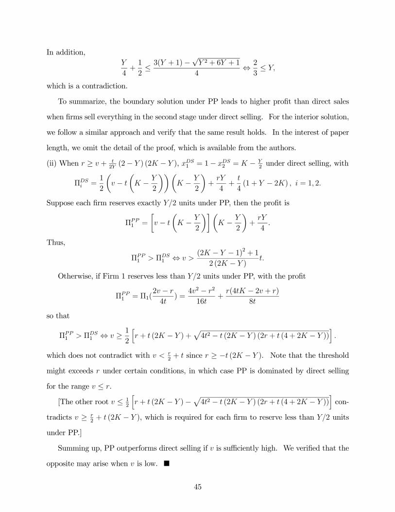
In addition,

4+1

2≤ 3( + 1)−

√ 2 + 6 + 1

4⇔ 2

3≤

which is a contradiction.

To summarize, the boundary solution under PP leads to higher profit than direct sales

when firms sell everything in the second stage under direct selling. For the interior solution,

we follow a similar approach and verify that the same result holds. In the interest of paper

length, we omit the detail of the proof, which is available from the authors.

(ii) When ≥ + 2(2− ) (2 − ),

1 = 1− 2 = −

2under direct selling, with

Π =

1

2

µ −

µ −

2

¶¶µ −

2

¶+

4+

4(1 + − 2) = 1 2

Suppose each firm reserves exactly 2 units under PP, then the profit is

Π1 =

∙ −

µ −

2

¶¸µ −

2

¶+

4.

Thus,

Π1 Π

1 ⇔ (2 − − 1)2 + 1

2 (2 − )

Otherwise, if Firm 1 reserves less than 2 units under PP, with the profit

Π1 = Π1(

2 −

4) =

42 − 2

16+

(4 − 2 + )

8

so that

Π1 Π

1 ⇔ ≥ 12

h + (2 − ) +

p42 − (2 − ) (2 + (4 + 2 − ))

i

which does not contradict with 2+ since ≥ − (2 − ). Note that the threshold

might exceeds under certain conditions, in which case PP is dominated by direct selling

for the range ≤ .

[The other root ≤ 12

h + (2 − )−

p42 − (2 − ) (2 + (4 + 2 − ))

icon-

tradicts ≥ 2+ (2 − ), which is required for each firm to reserve less than 2 units

under PP.]

Summing up, PP outperforms direct selling if is sufficiently high. We verified that the

opposite may arise when is low. ¥

45

Appendix B

Appendix B provides the derivation of the equilibria in the Extension and proofs for Propo-

sitions 6-7.

Less Competitive Environment 32

Posted Price

The analysis for the two cases under PP is the same as under ≥ 32. However, under

certain conditions Case 2 becomes valid. In particular, if (2− − ) ≤ (5 −1− 5

2 ), there exist multiple equilibria with 1 = 1− 2 ∈ [−(2−1− )

3 −

2]. This

solution requires ≥ 25+

2and ≥ 1

2+

4. Otherwise if (5 − 1 − 5

2 ) ≤

2+ 2( −

2), then 1 = 1 − 2 = −

2. This boundary solution holds when

≥ max© (2− 4 + 2 ) ¡5 − 1− 5

2¢ª. Finally, 1 = 1−2 = 2−

4if 2+2(−

2) ≤ 3

2, which requires ≤ (3− 4 + 2 ) and ≤ 3

8+

2.

Name-Your-Own-Price

The equilibrium under NYOP is similar to that under ≥ 32. When 9

22+

2

and 22−11−54

then there exist multiple equilibria with 1 = 1 −

2 ∈h−(2−2− )

74+(4+5−2 )

26

i. When 1

3+

2≤ ≤ 9

22+

2and 9− 9

2−2, there exist

multiple equilibria onh−(2−2− )

7 −

2

i. Otherwise, when +

¡4 − 1

2− 2 ¢,

then 1 = 1 −

2 = −4+ 1

8 and for ≤ +

¡4 − 1

2− 2 ¢, we have

1 =

1− 2 = −

2

Direct selling

In the second stage, if business demand is high, each provider behaves like a local monop-

olist and sells to postponers close to him as in the base model with ≥ 32. When business

demand is low, however, providers together will cover the entire leisure market. In this case,

the postponer at location e is indifferent between buying from Firm 1 or Firm 2:

e = 1

2+

2 −

1

2

Firm 1’s profit in the second stage is 1 (e− 1) where − e −

1 ≥ 0 is needed to

46

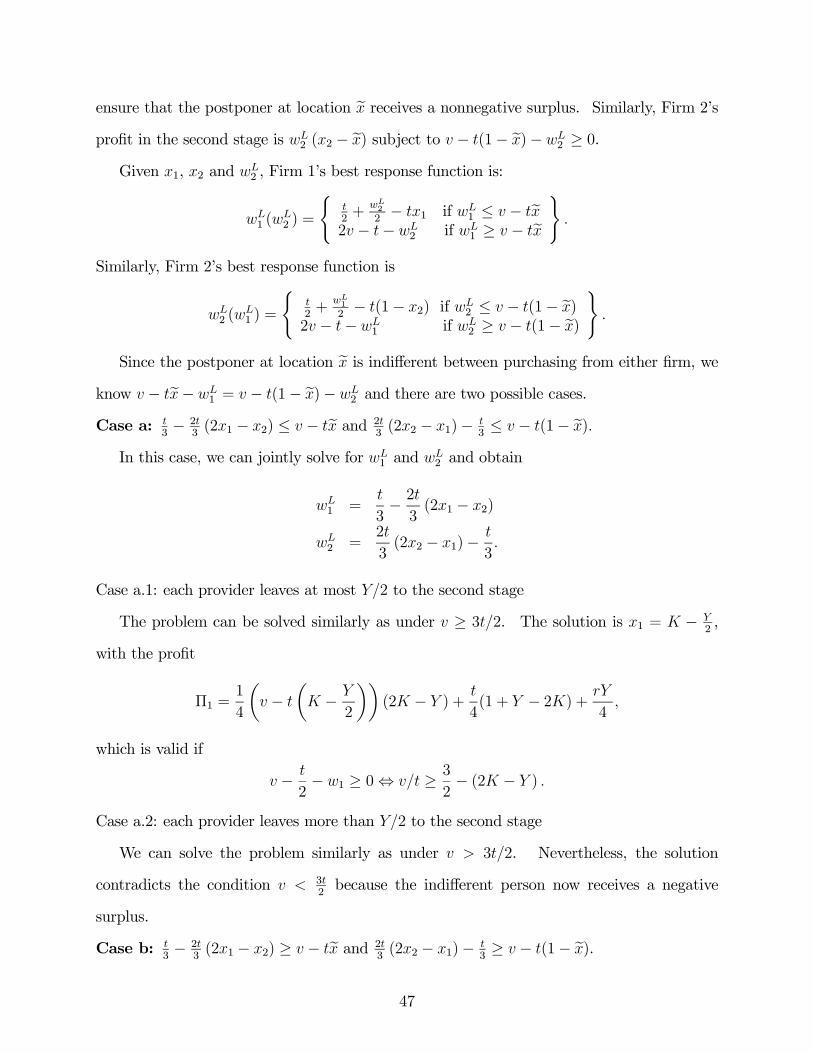
ensure that the postponer at location e receives a nonnegative surplus. Similarly, Firm 2’s

profit in the second stage is 2 (2 − e) subject to − (1− e)−

2 ≥ 0.Given 1, 2 and

2 , Firm 1’s best response function is:

1 (

2 ) =

(2+

22− 1 if

1 ≤ − e2 − −

2 if 1 ≥ − e

)

Similarly, Firm 2’s best response function is

2 (

1 ) =

(2+

12− (1− 2) if

2 ≤ − (1− e)

2 − − 1 if

2 ≥ − (1− e))

Since the postponer at location e is indifferent between purchasing from either firm, we

know − e− 1 = − (1− e)−

2 and there are two possible cases.

Case a: 3− 2

3(21 − 2) ≤ − e and 2

3(22 − 1)−

3≤ − (1− e)

In this case, we can jointly solve for 1 and

2 and obtain

1 =

3− 23(21 − 2)

2 =

2

3(22 − 1)−

3

Case a.1: each provider leaves at most 2 to the second stage

The problem can be solved similarly as under ≥ 32. The solution is 1 = − 2,

with the profit

Π1 =1

4

µ −

µ −

2

¶¶(2 − ) +

4(1 + − 2) +

4

which is valid if

−

2− 1 ≥ 0⇔ ≥ 3

2− (2 − )

Case a.2: each provider leaves more than 2 to the second stage

We can solve the problem similarly as under 32. Nevertheless, the solution

contradicts the condition 32because the indifferent person now receives a negative

surplus.

Case b: 3− 2

3(21 − 2) ≥ − e and 2

3(22 − 1)−

3≥ − (1− e).

47

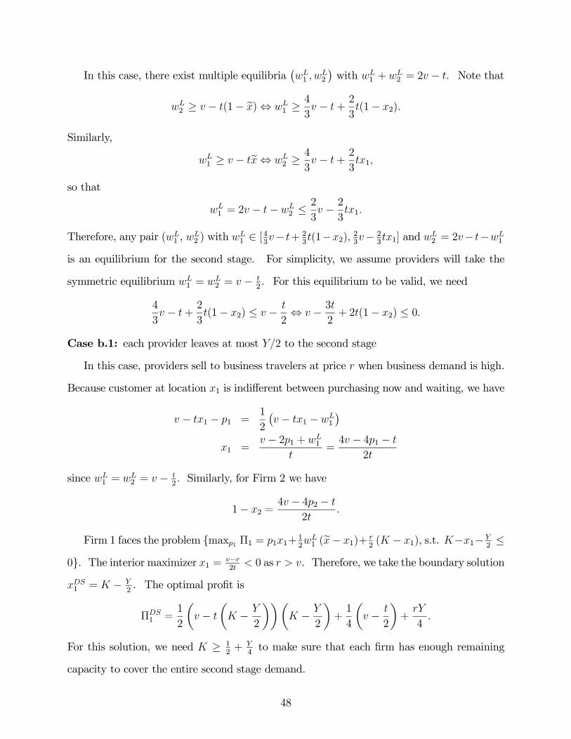
In this case, there exist multiple equilibria¡1

2

¢with

1 + 2 = 2 − . Note that

2 ≥ − (1− e)⇔

1 ≥4

3 − +

2

3(1− 2)

Similarly,

1 ≥ − e⇔

2 ≥4

3 − +

2

31

so that

1 = 2 − −

2 ≤2

3 − 2

31

Therefore, any pair (1 ,

2 ) with

1 ∈ [43− + 2

3(1−2) 23− 2

31] and

2 = 2− −

1

is an equilibrium for the second stage. For simplicity, we assume providers will take the

symmetric equilibrium 1 =

2 = − 2. For this equilibrium to be valid, we need

4

3 − +

2

3(1− 2) ≤ −

2⇔ − 3

2+ 2(1− 2) ≤ 0

Case b.1: each provider leaves at most 2 to the second stage

In this case, providers sell to business travelers at price when business demand is high.

Because customer at location 1 is indifferent between purchasing now and waiting, we have

− 1 − 1 =1

2

¡ − 1 −

1

¢1 =

− 21 + 1

=4 − 41 −

2

since 1 =

2 = − 2 Similarly, for Firm 2 we have

1− 2 =4 − 42 −

2

Firm 1 faces the problem {max1 Π1 = 11+121 (e− 1)+

2( − 1), s.t. −1−

2≤

0}. The interior maximizer 1 =−2

0 as . Therefore, we take the boundary solution

1 = −

2. The optimal profit is

Π1 =

1

2

µ −

µ −

2

¶¶µ −

2

¶+1

4

µ −

2

¶+

4

For this solution, we need ≥ 12+

4to make sure that each firm has enough remaining

capacity to cover the entire second stage demand.

48

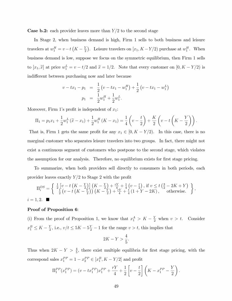
Case b.2: each provider leaves more than 2 to the second stage

In Stage 2, when business demand is high, Firm 1 sells to both business and leisure

travelers at 1 = − ¡ −

2

¢. Leisure travelers on [1−2) purchase at

1 . When

business demand is low, suppose we focus on the symmetric equilibrium, then Firm 1 sells

to [1 e] at price 1 = − 2 and e = 12. Note that every customer on [0 − 2) is

indifferent between purchasing now and later because

− 1 − 1 =1

2

¡ − 1 −

1

¢+1

2

¡ − 1 −

1

¢1 =

1

21 +

1

21

Moreover, Firm 1’s profit is independent of 1:

Π1 = 11 +1

21 (e− 1) +

1

21 ( − 1) =

1

4

µ −

2

¶+

2

µ −

µ −

2

¶¶

That is, Firm 1 gets the same profit for any 1 ∈ [0 − 2). In this case, there is no

marginal customer who separates leisure travelers into two groups. In fact, there might not

exist a continuous segment of customers who postpone to the second stage, which violates

the assumption for our analysis. Therefore, no equilibrium exists for first stage pricing.

To summarize, when both providers sell directly to consumers in both periods, each

provider leaves exactly 2 to Stage 2 with the profit

Π =

½12

£ −

¡ −

2

¢¤ ¡ −

2

¢+

4+ 1

4

¡ −

2

¢, if ≤

¡32− 2 +

¢12

¡ −

¡ −

2

¢¢ ¡ −

2

¢+

4+

4(1 + − 2) , otherwise.

¾

= 1 2. ¥

Proof of Proposition 6:

(i) From the proof of Proposition 1, we know that 1 − 2when . Consider

1 ≤ − 2, i.e., ≤ 5 − 5

2− 1 for the range , this implies that

2 − 4

5

Thus when 2 − 45, there exist multiple equilibria for first stage pricing, with the

correspond sales 1 = 1− 2 ∈ [1 − 2] and profit

Π1 (1 ) = ( − 1 )1 +

4+1

2

∙ −

2

¸µ − 1 −

2

¶

49

The collusive outcome is greater than − 2if ≥

¡4 − 1

2− 2 ¢. Also, for 1

not to exceed − 2we need ≤

¡5 − 1− 5

2¢. Combining these two inequalities yields

µ4 − 1

2− 2

¶≤

µ5 − 1− 5

2

¶⇔ 2 − 1− ≥ 0

which violates our basic assumption. Therefore, when multiple equilibria exist under PP, the

collusive outcome must be either lower than 1 or within£1 −

2

¤. By unimodality

of Firm 1’s profit function under symmetric strategies, the lowest equilibrium profit can only

be achieved at − 2or 1 . Note that

Π1(1 ) ≥ Π1

µ −

2

¶⇔ ≤

µ5 − 1− 5

2

¶or ≥

2(4 + 1− 2 )

Since 1 ≤ − 2implies ≤

¡5 − 1− 5

2¢, the lowest profit is achieved at −

2when

multiple equilibria exist under PP.

(ii) In the proof of Proposition 4, we have shown that if Case 1 is optimal under PP, the

competing providers prefer the PP over the NYOPmechanism. The proof applies to

32as well. When 3

2, it is possible for Case 2 to be optimal so that multiple equilibria

exist under the PP mechanism, in which case the lowest profit is achieved at − 2. The

highest possible profit under NYOP is reached at the collusive decision, =

8+ 3

16.

Π1

µ −

2

¶≥ Π

1

µ

8+3

16

¶ ≥

µ3

2(16 − 1− 8 )− 4

√2p(2 − ) (8 − 1− 4 )

¶and

≤

µ3

2(16 − 1− 8 ) + 4

√2p(2 − ) (8 − 1− 4 )

¶However, the existence of multiple equilibria under NYOP requires ≤

¡9 − 2− 9

2¢

and consequently, ≥ 13+

2. Note that

µ9 − 2− 9

2

¶≤

µ3

2(16 − 1− 8 ) + 4

√2p(2 − ) (8 − 1− 4 )

¶always holds. Also, note that ≥

³32(16 − 1− 8 )− 4√2

p(2 − ) (8 − 1− 4 )

´.

To see that, if suffices to show

0 ≥

µ24 − 5

2− 12 − 4

√2p(2 − ) (8 − 1− 4 )

¶

50

Since ≥ 13+

2, we have

4√2p(2 − ) (8 − 1− 4 ) ≥ 24 − 5

2− 12 ≥ 0

7− 2√616

+

2≤ ≤ 7 + 2

√6

16+

2

Since 7+2√6

16≥ 1

2and 7−2√6

16≤ 1

3, this inequality is always satisfied when there exist multiple

equilibria under NYOP.

(iii) First consider the case ≤ ¡32− 2 ¡ −

2

¢¢, which implies ≤ 1

4+

2(which also

implies ≥ 1 as ≥ 12+

4has to hold). In this range, the profit under direct selling is

Π1 =

1

2

µ −

µ −

2

¶¶µ −

2

¶+

4+1

4

µ −

2

¶

For ≤ 14+

2, only Case 1 can arise under PP. First consider ≥

2+ (2 − ) so

that it is optimal to leave less than 2 units under PP, i.e.,

Π1 ≥ Π

1

µ2 −

4

¶ ≥ 1

2

³ + (1 + 2 − )−

p (1− 2 + ) (2 − (1− 2 + ))

´and

≤ 1

2

³ + (1 + 2 − ) +

p (1− 2 + ) (2 − (1− 2 + ))

´The first inequality always holds because ≥

2+ (2 − ) and ≥ ≥ (1− 2 + ).

Regarding the second inequality, it suffices to show

≤ 12

³ + (1 + 2 − ) +

p (1− 2 + ) (2 − (1− 2 + ))

´

µ2−√2

q1− (−2 + )

2

¶≤ ≤

µ2 +√2

q1− (−2 + )

2

¶

The first inequality is satisfied by the fact that ≥ as it leads to 2−√24≤ ≤

2+√24

which is always satisfied as 2≤ ≤

2+ 1

4. For the second inequality, note that ≤

(3− 4 + 2 ) is needed to have the interior solution under PP. This implies the second

inequality if and only if 2−

√10−212≤ ≤

2+√10+212

, which holds since 2≤ ≤

2+ 1

4.

Thus direct selling dominates PP when 2+ (2 − ) ≤ ≤

¡32− 2 ¡ −

2

¢¢.

51

We next consider the boundary solution under PP, where each provider leaves Y/2 units

to the second stage. Then

Π1 ≥ Π

1

µ −

2

¶⇔ ≥

2(1 + 2 − )

which always holds as ≥ . Therefore, direct selling dominates PP when ≤¡32− 2 +

¢.

For ¡32− 2 +

¢ ≤ 32, the profit under direct selling is

Π1 =

1

2

µ −

µ −

2

¶¶µ −

2

¶+

4+

4(1 + − 2)

Following a similar approach, we verified that direct selling dominates PP when is suffi-

ciently low, whereas the opposite may arise when is high enough. In the interest of length,

we omit the details of the proof, which are available from the authors. ¥

Multiple Resellers

a) Two Posted Price Resellers

There are two cases when firms sell through two PP resellers.

Case 1: Each provider leaves at most 2 units to the second stage

With two opaque resellers, postponers purchase from the reseller who offers the lower

price. When business demand is low in Stage 2, competition leads to 1 =

2 = 0 and

providers split the demand equally. As postponers can buy from either reseller, competition

in the resale market leads to 1 = 2 = 0. As a result, resellers make no profit and

postponers retain a positive expected surplus of − 2. When business demand is high,

postponers receive a zero surplus. Let 1 denote the location of the leisure traveler who is

indifferent between purchasing from Firm 1 in Stage 1 and waiting. Then

− 1 − 1 =1

2

µ −

2

¶⇔ 1 =

2 + − 414

Firm 1 faces a profit maximization problem:

max1

Π1 = 11 + ( − 1)

2

− 1 ≤

2

52

Firm 2 faces a similar problem in deciding 2. The equilibrium solution is identical to that

of Case 1 with a single NYOP reseller.

Case 2: Each provider leaves more than 2 units to the second stage

In Stage 2, if business demand is low, we obtain the same result as in Case 1 with = 0

and = 0. Otherwise if business demand is high, Firm 1 has −1− 2units and Firm 2

has − (1− 2)− 2units after satisfying the business demand. The competition between

the resellers leads them to price at the margin, i.e.,

1 =

2 = 1 = 2

= − − (1− 2)−

2

2 − 1 − (1− 2)− −

1− 1 − 2

2 − 1 − (1− 2)− (2 − (1− 2)− )

Again, let denote the location of the leisure traveler who is indifferent between purchasing

from Firm in Stage 1 and waiting. The leisure traveler at location 1 expects a surplus

(1− 1 − 2) under high business demand and − 2under low business demand, i.e.,

− 1 − 1 =1

2

µ −

2

¶+

2(1− 1 − 2)

whereas for 2

− (1− 2)− 2 =1

2

µ −

2

¶

Jointly solving for 1 and 2 yields:

1 =2 + − 81 + 42

4

1− 2 =2 + − 42

4

Firm 1 faces the problem:

max1

Π1 = 11 +

4+1

41

µ − 1 −

2

¶+1

41

µ − 1 + 2 −

2

¶ − 1 ≤

2

Firm 2 faces a similar problem in deciding 2. Solving these two problems yields the

equilibrium solution under Case 2.

53

We then compare the two cases to obtain the equilibrium solution. For , 21 =

1 − 22 = −4+ 1

8if ≥ + (4 − 1

2− 2 ). This solution requires 1

8+

2.

Otherwise if + (4 − 12− 2 ), we have 21 = 1 − 22 = −

2, which holds

when ≥ (3 + 4 − 8). When ≥ 310+

2, each provider leaves more than 2 units

to the second stage, and there exist multiple equilibria. In particular, if 1118 + 9,

21 = 1 − 22 ∈ [3−4+26

4−2+314

]. Otherwise when ≤ 1118 + 9, there exist

multiple equilibria on [3−4+26

− 2]. Note that we need ≥ 3

2− so that each

provider is able to individually cover all postponers’ demand when business demand is low,

at least for the lowest equilibrium solution 1 =3−4+2

6.

With two competing PP resellers, resellers make no profit due to the fierce competition

created by product opaqueness. Postponers expect a higher surplus from Stage 2 compared

to the case of one reseller. This makes providers worse off compared to selling via a single

PP reseller.

b) Two NYOP Resellers

Suppose there are two competing NYOP resellers. Due to the passive role of resellers

under the NYOPmechanism, results with multiple resellers are the same as in the case of one

NYOP reseller, except that the two resellers will split the positive profit, if any, generated

from the NYOP channel.

c) One PP Reseller and one NYOP reseller

Suppose there are two competing resellers, one using the PP mechanism and the other

using the NYOP mechanism. In this case, the postponers are able to infer the state of

business demand from the price set by the PP reseller. Therefore, when business demand

is low, postponers anticipate 1 =

2 = 0 and they bid at = 0 in the NYOP channel.

Facing the competition from the NYOP reseller, the PP reseller is forced to set a price equal

to zero. When business demand is high, if each provider reserves less than 2 units to

Stage 2, the resale market is not active. Otherwise if there is still capacity after satisfying

the business demand, postponers infer service providers’ wholesale prices by observing the

54

price of the PP reseller. Since postponers in the range [1 b] (where b = 2− (1−2)− )submit a bid equal to the wholesale prices, the PP reseller is forced to set a price equal to

the wholesale prices as well. Therefore, providers receive the same profit as selling via two

opaque PP resellers.

Proof of Proposition 7: For this proof we consider .

(i) Note that if Case 1 is optimal with two PP resellers, then Case 1 is optimal under a single

PP as 1 ≥ 21 .

(i.a) First consider Case 1 is optimal under two PP resellers. Recall that Firm 1’s profit

function under a single PP reseller is given by

Π1 (1) = ( − 1)1 +

( − 1)

2 1 ≥ −

2.

Firm 1’s profit function under 2PP is

Π21 (1) =

∙ − 1 − 1

2

µ −

2

¶¸1 +

( − 1)

2 1 ≥ −

2

Since −1 ≥ −1− 12

¡ −

2

¢, we have Π

1 (21 ) ≥ Π21 (21 ). Because 1 max-

imizes Π1 (1) and

1 ≥ 21 ≥ −

2, we have Π

1 (1 ) ≥ Π1 (21 ) ≥ Π21 (21 ).

So if Case 1 is optimal under both PP and 2PP, the profit is higher under a single PP.

(i.b) Suppose Case 2 is optimal under two PP resellers, whereas Case 1 is optimal with a

single PP reseller.

With a single PP reseller, Case 1 is optimal if ≥ ¡5 − 1− 5

2¢. It suffices to compare

the highest profit obtainable under 2 PP in Case 2 with a feasible solution, Π1 ( −

2) =£

− ¡ −

2

¢¤ ¡ −

2

¢+

4under single PP reseller. The highest profit in Case 2 with

two PP resellers is

Π21 (21 ) =

∙ − 21 − 1

2

µ −

2

¶¸21 +

4+1

2

µ −

2

¶µ − 21 −

2

¶

where 21 = 14if ≥ 3

8+

2or 21 = 3−4+2

6if ≥ max©3

2− ; 3

10+

2

ª.

Suppose 21 = 14. Then, Π

1 ( − 2) ≥ Π21 (1

4) iff ≥

2(4 − 1− 2 ) +

4

¡1

2−¢,

which is implied by ≥ ¡5 − 1− 5

2¢if

≤ 1−√7

12+

2and ≥ 1 +

√7

12+

2

55

The first inequality is never satisfied as ≥ 2, whereas the second inequality always holds

because ≥ 38+

2.

Suppose 21 = 3−4+26

. Then, Π1 ( −

2) ≥ Π21 (3−4+2

6) if and only if ≥

18(20 + 3− 10 ), which is implied by ≥

¡5 − 1− 5

2¢if and only if ≥ 3

10+

2

which always holds here.

i.c) Finally, we consider that Case 2 arises under both a single and two PP resellers. In

this case, 1 = − 2is an equilibrium solution that gives the lowest profit among all

the equilibria points under a single PP reseller. This profit will dominate the highest profit

achieved under 2 PP. In fact, Π1 (−

2) ≥ Π21 (1

4) if and only if ≥

2(4 − 1− 2 )+

4

¡1

2−¢, which is always implied by ≥ since 3−√5

8+

2≤ ≤ 3+

√5

8+

2holds when

≥ 310+

2and ≤ 1

2+

2.

(ii) The result follows immediately from the derivation of the case with multiple competing

NYOP resellers.

(iii) The equivalence of selling via two competing PP resellers and selling via one PP and one

NYOP reseller follows immediately from the derivation of the latter case. We now compare

selling via 2 PP resellers with selling via one NYOP reseller (which is equivalent to selling

via multiple NYOP resellers).

(iii.a) Suppose Case 1 is optimal under both 2 PP and 1 NYOP. Then, it is straightforward to

see that the equilibrium profits are the same because the equilibrium solutions are identical.

(iii.b) Case 2 is optimal under at least one of the mechanisms.

For multiple equilibria to arise under NYOP we need, among other conditions, ≥ 13+

2,

which implies ≥ 310+

2 under which multiple equilibria arise when selling via 2 PP

resellers. Therefore, if Case 2 is optimal under NYOP, Case 2 must also be optimal under

2 PP resellers. We then have two possible cases:

(iii.b.1) Case 2 is optimal under both mechanisms, with the optimal profits

Π21 (21 ) =

∙ − 21 − 1

2

µ −

2

¶¸21 +

4+1

2

µ −

2

¶µ − 21 −

2

¶

56

and

Π1 (

1 ) =

∙ −

1 − 2 −

4

¸ 1 +

+¡ −

2

¢ ¡ −

1 − 2

¢4

respectively. Note that

3− 4 + 2

6≤ − (2 − 2− )

7⇔ 3

2− 8 − 4

3≤

which always holds for ≥ 310+

2. For any equilibrium

1 under NYOP, it is also an

equilibria under 2 PP, and Π21 (1 ) ≥ Π

1 (1 ).

(iii.b.2) Case 2 is optimal under 2 PP resellers, whereas 1 = 1− 2 = − 2under NYOP.

Here − 2 leads to the lowest profit among all the multiple equilibria under two PP

resellers, so Π21 (21 ) ≥ Π21 ( − 2) ≥ Π1 ( − 2). ¥

Mixed Strategy Equilibria

We now analyze the case where each provider is unable to fulfill the postponers’ demand

individually under low business demand, however the total capacity is sufficient to cover the

leisure segment, i.e., 2− 1 ≥ 0. In this case, equilibrium in pure strategy no longer exists.Due to the complexity of the full analysis, we show robustness of our results based on the

characterization of mixed strategy equilibrium at the symmetry, i.e., 1 = 1− 2 = , when

it is optimal for each provider to leave at most 2 to Stage 2. The resale market is active

only when business demand is low, and we suppress the superscript “” for here.

The PP mechanism

Under the PPmechanism, in the mixed strategy equilibrium is chosen from the support

[] according to the cumulative distribution () and density (). Clearly, if 1

2 Firm 1 sells − and Firm 2 sells 1 − − , and vice versa when 1 2, whereas

the probability that 1 = 2 is zero as () has no mass point. For every , the profit

Π1 () obtained by Firm 1 from leisure travelers in Stage 2 is:

Π1 () = [(1− 2 ()) ( − ) + 2 () (1− − )] = constant.

and, similarly, for Firm 2:

Π2 () = [(1− 1 ()) ( − ) + 1 () (1− − )] = constant.

57

At the extremes of the support, Firm 1’s profit expression:

Π1 () = (1− − ) = Π1

Π1 () = ( − ) = Π1

Similar expression can be obtained for Firm 2. Given the symmetry, the maximum price

that postponers are able to pay when = 0 is = − 2. Therefore,

Π1 = Π

2 = (1− − )

µ −

2

¶

=(1− − )

¡ −

2

¢ −

Note that ≥ holds as by hypothesis 2− 1 ≥ 0. The common cumulative distribu-tion from which wholesale prices are drawn and the relative density are:

() =1

2 − 1

"( − )− (1− − )

¡ −

2

¢

#,

() =(1− − )

¡ −

2

¢( − )2

for ≤ ≤ . Therefore, under PP the service providers make a positive profit.

The NYOP mechanism

Since each provider leaves at most 2 to Stage 2, postponers’ bidding strategy is aimed

at obtaining the service only when business demand is low. Furthermore, because of the

symmetry and the presence of the opaque reseller, all the postponers have the same expected

surplus and the reseller expects them to make the same bid . If a mixed strategy exists any

wholesale price higher than this common bid yields a profit equal to zero to the providers

since the reseller will never sell if the bid is lower than the wholesale price. Therefore, if

[] is the support of the distribution of wholesale prices, it follows that = . Consider

postponer who decides to offer different than . If ≥ , postponer obtains the

service and his expected surplus is equal to − 2− . Otherwise, if , postponer

obtains the service only if at least one of the two providers sets a wholesale price lower

than , that is min (1 2) ≤ . Since the service providers choose the wholesale price

58

from the support [], where = is the common bid chosen by all the leisure travelers

except who is considering a lower bid, the probability of this event is:

Pr [min (1 2) ≤ ] = 1− [1− ()]2= () (2− ())

Therefore, if , the expected surplus of the postponer is:

[] =

µ −

2−

¶ () (2− ())

Summing up, postponer faces the following maximization problem:

max

½ ¡ −

2−

¢ () (2− ()) if = ¡

− 2−

¢if ≥ =

Solving this problem yields two possible solutions

∗ = −

2− () (2− ())

2 () (1− ())if =

∗ = = if ≥ =

Note that if = the optimal solution is less than − 2and less than , i.e., each

postponer will make a bid lower than with an expected surplus higher than − 2− .

Therefore, bidder lowers her bid below . Since each postponer has similar incentives

to cut her bid, unraveling leads to the equilibrium = = 0. As a consequence, under

NYOP, 1 = 2 = 0 and Π1 = Π

2 = 0.

Recall that under PP, providers make positive profits in Stage 2. Similar to the base

case, since postponers can expect a higher surplus in Stage 2 when the reseller utilizes the

NYOP mechanism, the prices set in Stage 1 will be lower under NYOP leading to lower

overall profit. Therefore, even in presence of a more restrictive capacity, contracting with a

reseller who uses the PP mechanism is more profitable for service providers.

For the comparison between PP and direct selling, note that the presence of capacity

constraints reduces the competition between providers compared to the base case. As a

result, using an opaque PP intermediary is more likely to be beneficial for providers than a

direct selling strategy.

59