open access visualizing the impact of storm …jnapiera/cv_files/... · river, which drains into...

The Open Geography Journal, 2010, 3, 131-147 131

1874-9232/10 2010 Bentham Open

Open Access

Visualizing the Impact of Storm Events on the Quality of the Buffalo and Niagara Rivers (NY)

Jacob Napieralski*,1

and Gordon Fraser2

1Department of Natural Sciences, University of Michigan- Dearborn, 4901 Evergreen Road, Dearborn, MI 48128, USA

2Great Lakes Center, Buffalo State College, 1300 Elmwood Avenue, Buffalo, NY 14222, USA

Abstract: Combined sewer overflows (CSOs) negatively affect water quality in urban river and lake systems worldwide

by contributing thermally enhanced waters, particulates, and various organic and inorganic contaminants. Cities that

utilize CSOs must reassess aging sewer systems or minimize the impact overflows have on water quality. The Buffalo

River, which drains into northeastern Lake Erie, receives contaminants from various chemical, metallurgical, and

petroleum industries. Rainfall events initiate discharge from over 40 CSOs located along the River and Canal shoreline

and are known to mobilize contaminated bed sediments. Therefore, this paper will illustrate how empirically derived

visualizations can characterize the geographic extent and parameterize effluent from CSOs and storm-induced suspended

sediment. We used oceanographic profilers and a three-dimensional visualization software package (EVS-Pro) to collect

and analyze water quality data and to create visual models of parameter responses to rainfall events and baseflow. The

visualizations (a) captured a distinct “first flush” from CSOs and the River, characterized as plumes of thermally

enhanced water, high in turbidity and low in dissolved oxygen, (b) revealed a well-defined westward trend of cooling

water and decreasing suspended sediment, away from the urban area, and (c) indicated suspended sediments departing the

mouth of the Buffalo River settle quickly. The combination of intense field monitoring with dataloggers and visualizations

revealed large-scale patterns and discriminated localized departures from these patterns, which can help predict sediment

sinks and sources, map the geographic dispersion of effluent matter, and guide remediation efforts.

Keywords: First flush, water quality monitoring, combined sewer overflows (CSOs), visualizations, storm event.

INTRODUCTION

Due to rapid urbanization and industrialization during the 20

th century, the practice of combining sanitary wastewater

with storm water (i.e. combined sewer overflows; CSOs) increased dramatically, especially within the Great Lakes Basin (Fig. 1). The United States Environmental Protection Agency [1] estimates CSO discharges occur approximately 50-80 times, release 4.5 x 10

9 m

3 of waste water and runoff

every year, and affect more than 40 million residents in the U.S alone. Storm events producing as little as 2.55 mm of precipitation can accumulate wastewater and runoff in these combined sewer systems [2]. During baseflow conditions, sediment and debris collect in the system and are discharged during the “first flush” of a run-off producing storm event [3-5]. Understanding the nature and distribution of these first flushes, as well as the impact of the entire overflow, is critical to the remediation of the Great Lakes and other large lake systems and urban waterways.

These same storm events may also resuspend bed sediments in the Great Lakes, many of which are contaminated or high in enteric and fecal bacteria [6-8]. Recent studies have focused the behavior and nature of storm-induced resuspension events, including the frequency

*Address correspondence to this author at the Department of Natural

Sciences, University of Michigan- Dearborn, 4901 Evergreen Road,

Dearborn, MI 48128, USA; Tel: 313-593-5157;

E-mail: [email protected]

of and meteorological conditions that cause storm-waves strong enough to resuspend shallow and deep sediments within the Great Lakes [9-13]. Even during baseflow conditions, ship traffic can have a significant disturbance on bed sediments, diminishing the quality of the overlying water column and degrading the aquatic ecosystem [7, 14]. As with CSOs, the resuspension of potentially contaminated bed sediments has a detrimental impact on human and aquatic health and complicates remediation efforts of urban waterways.

However, a key limitation in studying storm-induced sediment resuspension and overflows or discharge points, is the inability to rapidly gather sufficient water quality and sediment data because of the time and expense involved in collecting and analyzing samples in large bodies of water. To some degree, remote sensing techniques (e.g. correlating irradiance reflectance and mineral suspended sediment [15]) address the problem by allowing investigators to gather information over large areas quickly and relatively inexpensively. But remote sensing data provide only indirect measures of properties that need to be ground-truthed and calibrated in order to be applied with confidence. Furthermore, the ability of remote sensing data to infer deep structures within large water bodies is limited by the array of assumptions and water conditions that are required for application.

132 The Open Geography Journal, 2010, Volume 3 Napieralski and Fraser

Fig. (1). Map of study area location and distribution of sampling sites.

Visualizing the Impact of Storm Events The Open Geography Journal, 2010, Volume 3 133

The introduction of automated electronic data loggers has somewhat alleviated this problem because they acquire data at discrete intervals in fractions of a second and store it for downloading. For example, the Seabird CTD data logger collects data on a wide variety of parameters one to two orders of magnitude faster than other frequently used data loggers. Seabird data loggers can efficiently profile conductivity, temperature, density, PAR, dissolved oxygen, and salinity [16-19] in large water bodies. Similar data loggers (e.g. TSI 6500 sond) are also capable of gathering data rapidly and producing profiles of a variety of deployments. Automated data loggers, however, provide only part of the answer to the problem of describing the three-dimensional structure of large water bodies. Each sampling location is still only a discrete point that is a miniscule representation of the areal distribution of the various parameters that characterize a large water mass [20, 21]. Even with many such points, the variation is still difficult to visualize in 3D, in part because the data return may be too large to easily assimilate and visualize. Three-dimensional visualization software, therefore, is the other part of the solution because it allows marine scientists to enter data into three-dimensional space to correlate among the data points so that the parameter variability within the

total volume of the water mass can be visualized. Environmental Visualization Systems (EVS-Pro), one example of many three-dimensional visualization software packages, combines state-of-the-art analysis and visualization tools that can be integrated with modular analysis and graphics routines for customized visualization applications. Digital data from the Seabird can be quickly processed for display as fully-bounded and color-mapped three-dimensional isovolumes and color isolines, exploded layers of selected value intervals, and interactively positioned horizontal and vertical slice planes. All views are capable of rotation and translation in real-time to achieve optimum viewing perspectives [22].

The combined technologies of data loggers and visualizations have been used to determine static three-dimensional structures of large water bodies. Fraser et al. [22] modeled temperature variability spatial variability within Lake Erie and the U.S. National Oceanic and Atmospheric Administration (NOAA) combined these technologies to develop visualizations of the Chukchi Sea (unpublished data). While the development of 3D software, such as EVS-Pro is of interest to physical geographers [23], other applications include soil contamination, simulations of

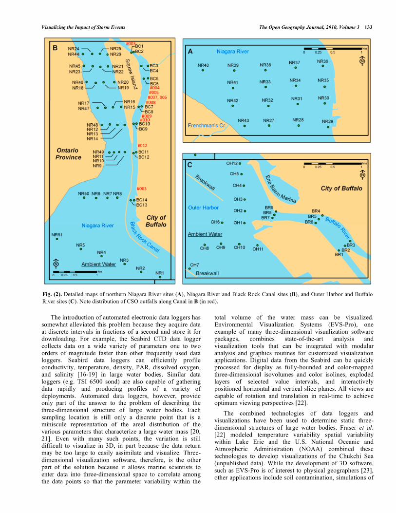
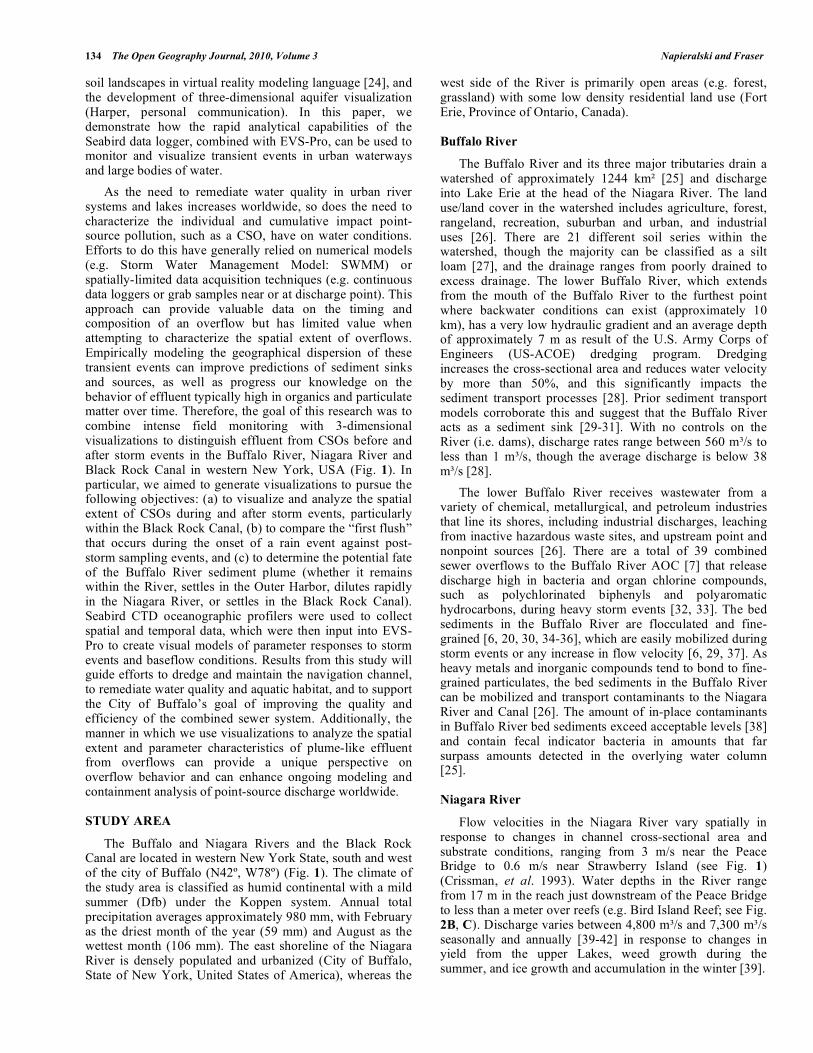
Fig. (2). Detailed maps of northern Niagara River sites (A), Niagara River and Black Rock Canal sites (B), and Outer Harbor and Buffalo

River sites (C). Note distribution of CSO outfalls along Canal in B (in red).


soil landscapes in virtual reality modeling language [24], and the development of three-dimensional aquifer visualization (Harper, personal communication). In this paper, we demonstrate how the rapid analytical capabilities of the Seabird data logger, combined with EVS-Pro, can be used to monitor and visualize transient events in urban waterways and large bodies of water.

As the need to remediate water quality in urban river systems and lakes increases worldwide, so does the need to characterize the individual and cumulative impact point-source pollution, such as a CSO, have on water conditions. Efforts to do this have generally relied on numerical models (e.g. Storm Water Management Model: SWMM) or spatially-limited data acquisition techniques (e.g. continuous data loggers or grab samples near or at discharge point). This approach can provide valuable data on the timing and composition of an overflow but has limited value when attempting to characterize the spatial extent of overflows. Empirically modeling the geographical dispersion of these transient events can improve predictions of sediment sinks and sources, as well as progress our knowledge on the behavior of effluent typically high in organics and particulate matter over time. Therefore, the goal of this research was to combine intense field monitoring with 3-dimensional visualizations to distinguish effluent from CSOs before and after storm events in the Buffalo River, Niagara River and Black Rock Canal in western New York, USA (Fig. 1). In particular, we aimed to generate visualizations to pursue the following objectives: (a) to visualize and analyze the spatial extent of CSOs during and after storm events, particularly within the Black Rock Canal, (b) to compare the “first flush” that occurs during the onset of a rain event against post-storm sampling events, and (c) to determine the potential fate of the Buffalo River sediment plume (whether it remains within the River, settles in the Outer Harbor, dilutes rapidly in the Niagara River, or settles in the Black Rock Canal). Seabird CTD oceanographic profilers were used to collect spatial and temporal data, which were then input into EVS-Pro to create visual models of parameter responses to storm events and baseflow conditions. Results from this study will guide efforts to dredge and maintain the navigation channel, to remediate water quality and aquatic habitat, and to support the City of Buffalo’s goal of improving the quality and efficiency of the combined sewer system. Additionally, the manner in which we use visualizations to analyze the spatial extent and parameter characteristics of plume-like effluent from overflows can provide a unique perspective on overflow behavior and can enhance ongoing modeling and containment analysis of point-source discharge worldwide.

STUDY AREA

The Buffalo and Niagara Rivers and the Black Rock Canal are located in western New York State, south and west of the city of Buffalo (N42º, W78º) (Fig. 1). The climate of the study area is classified as humid continental with a mild summer (Dfb) under the Koppen system. Annual total precipitation averages approximately 980 mm, with February as the driest month of the year (59 mm) and August as the wettest month (106 mm). The east shoreline of the Niagara River is densely populated and urbanized (City of Buffalo, State of New York, United States of America), whereas the

west side of the River is primarily open areas (e.g. forest, grassland) with some low density residential land use (Fort Erie, Province of Ontario, Canada).

Buffalo River

The Buffalo River and its three major tributaries drain a watershed of approximately 1244 km [25] and discharge into Lake Erie at the head of the Niagara River. The land use/land cover in the watershed includes agriculture, forest, rangeland, recreation, suburban and urban, and industrial uses [26]. There are 21 different soil series within the watershed, though the majority can be classified as a silt loam [27], and the drainage ranges from poorly drained to excess drainage. The lower Buffalo River, which extends from the mouth of the Buffalo River to the furthest point where backwater conditions can exist (approximately 10 km), has a very low hydraulic gradient and an average depth of approximately 7 m as result of the U.S. Army Corps of Engineers (US-ACOE) dredging program. Dredging increases the cross-sectional area and reduces water velocity by more than 50%, and this significantly impacts the sediment transport processes [28]. Prior sediment transport models corroborate this and suggest that the Buffalo River acts as a sediment sink [29-31]. With no controls on the River (i.e. dams), discharge rates range between 560 m /s to less than 1 m /s, though the average discharge is below 38 m /s [28].

The lower Buffalo River receives wastewater from a variety of chemical, metallurgical, and petroleum industries that line its shores, including industrial discharges, leaching from inactive hazardous waste sites, and upstream point and nonpoint sources [26]. There are a total of 39 combined sewer overflows to the Buffalo River AOC [7] that release discharge high in bacteria and organ chlorine compounds, such as polychlorinated biphenyls and polyaromatic hydrocarbons, during heavy storm events [32, 33]. The bed sediments in the Buffalo River are flocculated and fine-grained [6, 20, 30, 34-36], which are easily mobilized during storm events or any increase in flow velocity [6, 29, 37]. As heavy metals and inorganic compounds tend to bond to fine-grained particulates, the bed sediments in the Buffalo River can be mobilized and transport contaminants to the Niagara River and Canal [26]. The amount of in-place contaminants in Buffalo River bed sediments exceed acceptable levels [38] and contain fecal indicator bacteria in amounts that far surpass amounts detected in the overlying water column [25].

Niagara River

Flow velocities in the Niagara River vary spatially in response to changes in channel cross-sectional area and substrate conditions, ranging from 3 m/s near the Peace Bridge to 0.6 m/s near Strawberry Island (see Fig. 1) (Crissman, et al. 1993). Water depths in the River range from 17 m in the reach just downstream of the Peace Bridge to less than a meter over reefs (e.g. Bird Island Reef; see Fig. 2B, C). Discharge varies between 4,800 m /s and 7,300 m /s seasonally and annually [39-42] in response to changes in yield from the upper Lakes, weed growth during the summer, and ice growth and accumulation in the winter [39].


Black Rock Canal

The Black Rock Canal parallels the Niagara River from the Buffalo Harbor to the Black Rock Lock (see Figs. 1, 2). It is approximately 5.5 km long and 65 m wide at most points, and has a navigational channel depth of 7 m maintained by the U.S. Army Corp of Engineers. It is open to Lake Erie at its head, but is dammed by the locks at its mouth. Besides Lake Erie, its major water source is Scajaquada Creek, which has a mixed-use watershed size of 74 km

2. Water temperatures in

the Creek are typically higher than those in the Black Rock Canal, which results from its shallow depth and thermal enrichment from urban runoff [43].

Water from Lake Erie enters at the head of the Canal and through culverts in the breakwall separating the Canal from the Niagara River. The canal is adjacent to the New York State Thruway and receives storm runoff directly from the roadway drainage system. It also receives storm drainage from at least 9 major sewer outfalls (see Fig. 2B). Although through-flow in the Canal occurs only during the short time the locks at its mouth are opened for ship traffic, suspended sediment from the canal, which contains organic and inorganic contaminants, have been identified as far as Lake Ontario [44]. Although a channel depth of 7 m is maintained in the canal, shallow areas remain along the margins, and vegetation can be dense (e.g. opposite Bird Island Reef and along the shoreline and breakwall). Little research has been conducted on the Canal, though interest has increased recently regarding the impact of the Scajaquada Creek [43] and the influence of CSOs [21].

METHODOLOGY

Sampling Protocol

Sampling occurred at 85 sites: 14 within the Black Rock Canal (designated BC), 9 within the Buffalo River (BR), 11

in the Outer Harbor (OH), and 51 within the Niagara River (NR) (Fig. 2). These sample sites were aligned in 24 transects that had East-West orientations within the Black Rock Canal and Niagara River, and North-South orientations within the Buffalo River and the Outer Harbor. The same sample sites were used throughout the project. The x,y location was recorded using Magellan GPS units, and z location was established by pressure transducers on the profilers supplemented by depth recorders on the winch cables.

The sampling objective was to include storm events (SE) with rainfall of at least 12.5 mm and baseflow (BF) periods in which no precipitation occurred for at least 72 hours prior to sampling. Data collection occurred at all 85 sample sites once for each baseflow period and four times for the storm events, once 2 hours after the initial outset of the storm, then 6, 24, and 48 hours after the onset (Table 1). Sampling, however, occurred during only two storm events because (1) most rain events through the summer did not produce enough rain, (2) the intensity was not sufficient to overflow the sewers, or (3) some precipitation occurred during the 72 hours preceding the event. The characteristics of both storm events were generally similar, which included an initial period of intense rain, followed by brief pauses in precipitation, then less intense rainfall to conclude the storm (Table 2). The daily mean inflow to the Buffalo River Area of Concern was 73 m /s and 11 m /s at the start of SE 1 and 2, respectively, and 30 m /s and 11 m /s at the start of BF 1 and 2, respectively [21].

Data Collection

Two Seabird SBE Sea logger profilers were used to collect turbidity (FTUs), conductivity (μS/cm), depth (m), temperature (ºC), and dissolved oxygen (mg/l). Both data loggers were calibrated by Seabird before the project began

Table 1. Dates, Time, and Weather of Sampling Events

Sampling Event Temperature (°C) Rainfall (mm) Date Start Time (hh:mm)

Baseflow (BF) 1 15-20 --- May 9 10:00

Storm Event (SE) 1.1 17 19 June 9 13:00

Storm Event (SE) 1.2 16 --- June 9 19:00

Storm Event (SE) 1.3 15-20 10 June 11 13:30

Storm Event (SE) 2.1 19 18 August 23 8:00

Storm Event (SE) 2.2 19 --- August 23 14:00



Baseflow (BF) 2 15 --- September 7 11:00

Table 2. Characteristics of the Rainfall Events Sampled During the Study

Event Storm Duration

(hh:mm) Total Volume

(mm) Rainfall Intensity

(mm/h) Last Antecedent

Event (mm) Antecedent Dry

Time (Days) Return Period

(Months)

SE 1 3:07 19.56 6.60 9.65 3.2 2-3

SE 2 3:57 23.37 5.84 10.92 11.76 6


and had a precision of ±0.005 ºC for temperature and ±1.0 FTU for turbidity. The loggers were deployed simultaneously across the study area to increase sampling efficiency from the Great Lakes Center’s 40-foot research vessel, R/V Aquarius, and a 26-foot vessel, the R/V Pisces. Before each sampling run, the loggers were rinsed and weighted down to compensate for the fast current in the Niagara River. During deployment at a given site, the data logger was lowered within one meter of the riverbed and immediately raised back to the surface. Data reduction converted the data to 0.5 m depth intervals. Once at the surface, the loggers were deactivated to signal the completion of sampling at the site and to reset the logger for the next site. Every time a data logger was turned off, a cast was completed, and each time a cast was completed for all 85 sampling sites, a “run” was completed.

Data were collected during nine runs, seven during or after storm events and two during baseflow in the Buffalo River. Six parameters were measured for each run, and this resulted in a total of 108 separate visualizations, each from which slices could be extracted at any angle. For this study, turbidity and temperature were used to distinguish the Buffalo River plume from the ambient waters in Lake Erie and the Niagara River. Turbidity is a qualitative measure of suspended solids within the water column (a variable of key interest in this study), although this can be calibrated and converted to quantify sediment loadings. The correlation (r=0.88) between temperature and dissolved oxygen was statistically significant ( <0.05), meaning that visual models of dissolved oxygen would probably yield similar plume characteristics as visual models of temperature. Therefore, relying on temperature and turbidity reduced the number of models required to characterize the plumes. Comparisons are made between parameters at a particular sampling site and parameters of “ambient waters” (see Fig. 2). Ambient waters are generally those that are located away from outfalls, Rivers, or other contributing sources of turbidity and high temperatures. Thus, they represent conditions unaffected by potential impacts of outfalls. Sites NR4 and NR5 are particularly important for this use because they are relatively far from any shoreline and consistently reported results characteristic of levels commonly reported from the open waters of Lake Erie (e.g. turbidity <5.0 FTUs).

Irvine [21, 43] simultaneously and continuously monitored the impact of CSOs within the Buffalo River and Black Rock Canal using 10 Hydrolab IV Datasonde units, of which four were located within our study area. Results from Irvine during the same sampling periods provided reliable time series data for an accurate comparative analysis.

Data Processing

Environmental Visualization Systems (EVS-Pro) was used to generate 2- and 3-D visualizations of the data, isolating particular trends at discrete sites or transects. The interpolation methodology used by EVS-Pro, which utilizes ordinary kriging techniques (see [45] for specifics), originated from the interpolating methods developed by the U.S. EPA’s Geostatistical Environmental Assessment Software (Geo-EAS) to run 2- dimensional geostatistical analyses of spatially distributed data. EVS-Pro requires a 3-dimensional model of basin bathymetry to represent the

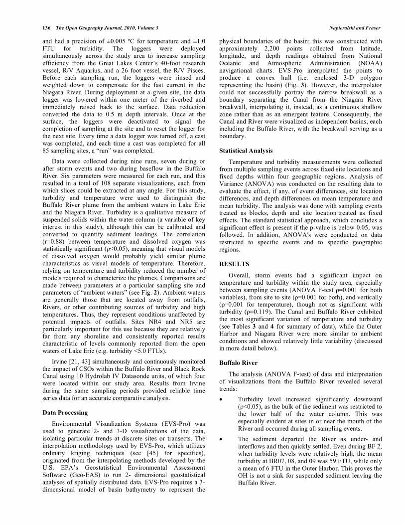
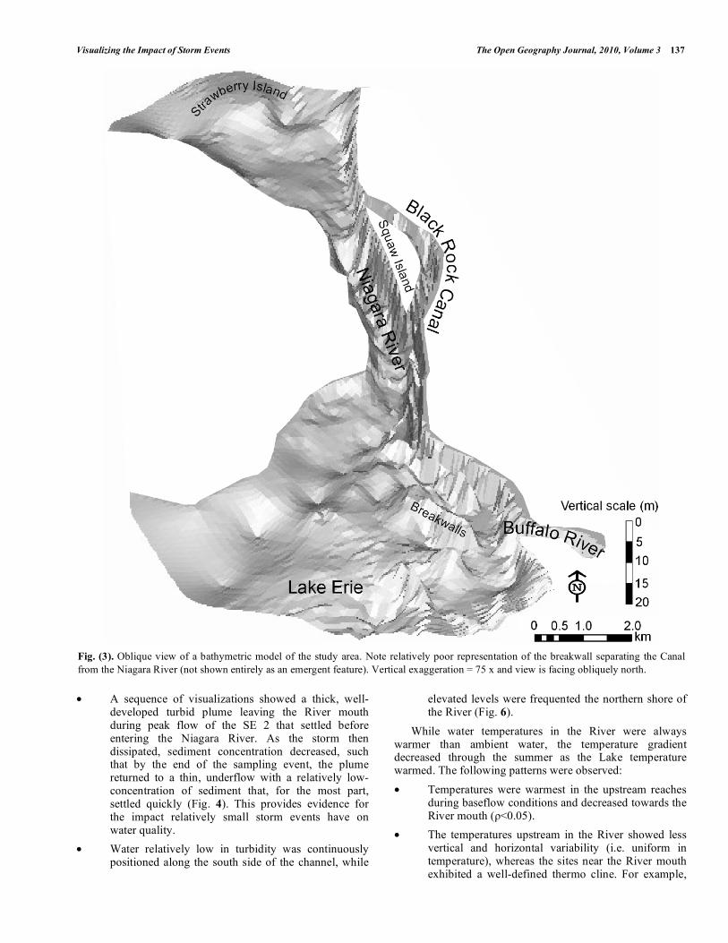
physical boundaries of the basin; this was constructed with approximately 2,200 points collected from latitude, longitude, and depth readings obtained from National Oceanic and Atmospheric Administration (NOAA) navigational charts. EVS-Pro interpolated the points to produce a convex hull (i.e. enclosed 3-D polygon representing the basin) (Fig. 3). However, the interpolator could not successfully portray the narrow breakwall as a boundary separating the Canal from the Niagara River breakwall, interpolating it, instead, as a continuous shallow zone rather than as an emergent feature. Consequently, the Canal and River were visualized as independent basins, each including the Buffalo River, with the breakwall serving as a boundary.

Statistical Analysis

Temperature and turbidity measurements were collected from multiple sampling events across fixed site locations and fixed depths within four geographic regions. Analysis of Variance (ANOVA) was conducted on the resulting data to evaluate the effect, if any, of event differences, site location differences, and depth differences on mean temperature and mean turbidity. The analysis was done with sampling events treated as blocks, depth and site location treated as fixed effects. The standard statistical approach, which concludes a significant effect is present if the p-value is below 0.05, was followed. In addition, ANOVA's were conducted on data restricted to specific events and to specific geographic regions.

RESULTS

Overall, storm events had a significant impact on temperature and turbidity within the study area, especially between sampling events (ANOVA F-test =0.001 for both variables), from site to site ( =0.001 for both), and vertically ( =0.001 for temperature), though not as significant with turbidity ( =0.119). The Canal and Buffalo River exhibited the most significant variation of temperature and turbidity (see Tables 3 and 4 for summary of data), while the Outer Harbor and Niagara River were more similar to ambient conditions and showed relatively little variability (discussed in more detail below).

Buffalo River

The analysis (ANOVA F-test) of data and interpretation of visualizations from the Buffalo River revealed several trends:

• Turbidity level increased significantly downward ( <0.05), as the bulk of the sediment was restricted to the lower half of the water column. This was especially evident at sites in or near the mouth of the River and occurred during all sampling events.

• The sediment departed the River as under- and interflows and then quickly settled. Even during BF 2, when turbidity levels were relatively high, the mean turbidity at BR07, 08, and 09 was 59 FTU, while only a mean of 6 FTU in the Outer Harbor. This proves the OH is not a sink for suspended sediment leaving the Buffalo River.


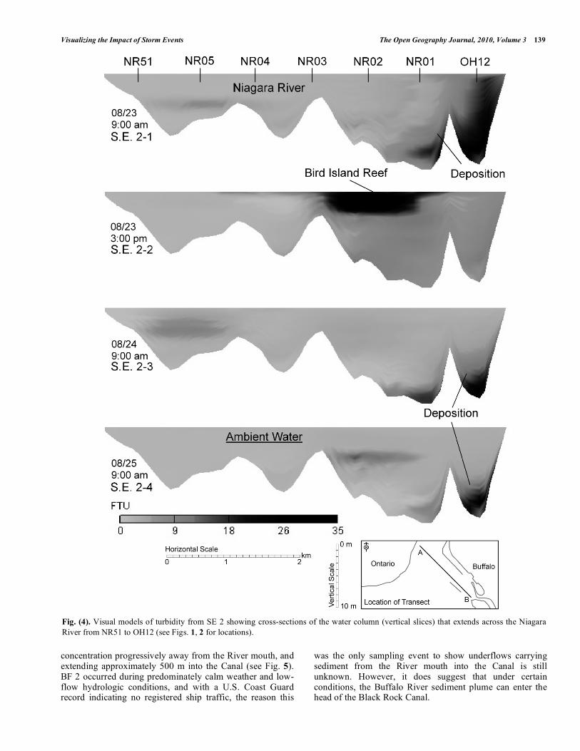
• A sequence of visualizations showed a thick, well-developed turbid plume leaving the River mouth during peak flow of the SE 2 that settled before entering the Niagara River. As the storm then dissipated, sediment concentration decreased, such that by the end of the sampling event, the plume returned to a thin, underflow with a relatively low-concentration of sediment that, for the most part, settled quickly (Fig. 4). This provides evidence for the impact relatively small storm events have on water quality.

• Water relatively low in turbidity was continuously positioned along the south side of the channel, while

elevated levels were frequented the northern shore of the River (Fig. 6).

While water temperatures in the River were always warmer than ambient water, the temperature gradient decreased through the summer as the Lake temperature warmed. The following patterns were observed:

• Temperatures were warmest in the upstream reaches during baseflow conditions and decreased towards the River mouth ( <0.05).

• The temperatures upstream in the River showed less vertical and horizontal variability (i.e. uniform in temperature), whereas the sites near the River mouth exhibited a well-defined thermo cline. For example,

Fig. (3). Oblique view of a bathymetric model of the study area. Note relatively poor representation of the breakwall separating the Canal

from the Niagara River (not shown entirely as an emergent feature). Vertical exaggeration = 75 x and view is facing obliquely north.


during SE 1.3, warm water can be visualized (using a series of horizontal slices of water temperature every 0.5 m) leaving the Buffalo River as a buoyant plume that veers left (north) into the Outer Harbor (Fig. 5).

• The visual models revealed a secondary flow caused by a second rainfall event that occurred during SE 1.3. The increase in water temperature (and suspended sediment) was not as significant as the “first flush” (SE 1.1); this can be attributed to the low rainfall amount and intensity (see Table 1).

Niagara River and Outer Harbor

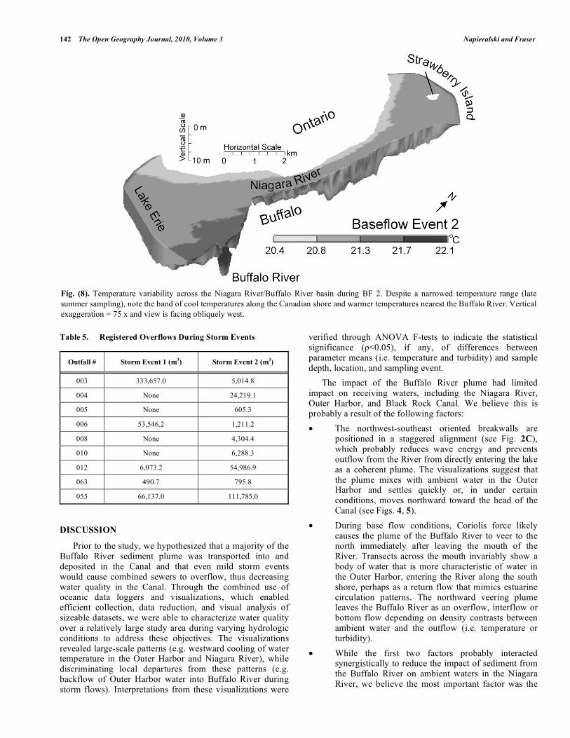
Turbidity within the Niagara River showed statistically significant horizontal variability (between sites) within the River ( <0.05) but no significant vertical variation ( >0.90). This corresponded with water temperature trends in the Niagara River: thoroughly mixed waters vertically (i.e. no thermocline) but significant variability between sites ( <0.05). Most of the horizontal variability was characterized by decreasing temperatures and turbidity from east to west (towards Canadian shore). During SE 1 (Fig. 7), the band of cool temperatures (3 °C cooler than those adjacent to the US shore) along the Canadian shore extended as much as 300 m from the shore. During SE 1.3, this same band of cool temperatures narrowed and was only 1 °C

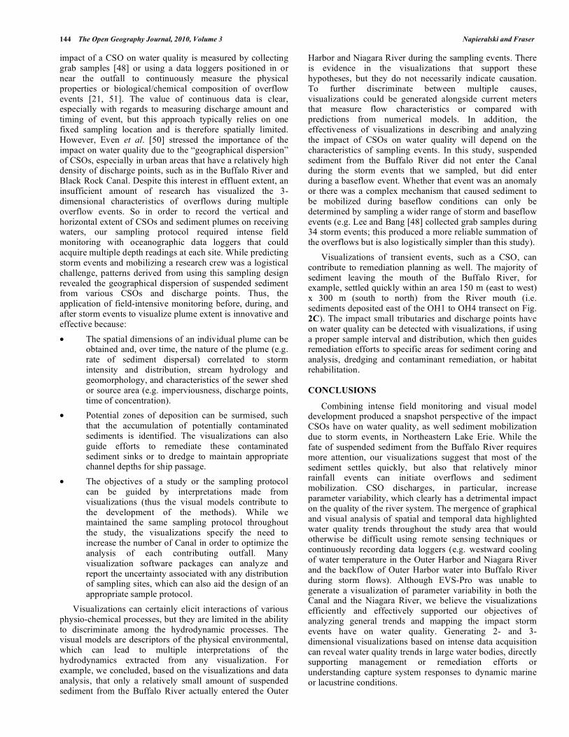
cooler than waters to the east. Even when the temperate gradient narrowed to 0.5 °C (i.e. SE 2), the well-developed trend of westward cooling was still evident on the visualizations (Fig. 8).

The Outer Harbor exhibited both horizontal and vertical variability during several sampling events (i.e. SE 1.1 and 1.2) for temperature and turbidity. A common characteristic observed during SE 2 was significant variability between sampling sites ( <0.05) but homogenous water vertically (0.758> <0.223) for both variables. This indicates that during storm events, effluent from the Buffalo River affected several OH sites near the mouth of the River but the impact the plume had on the overall vertical distribution of sediment and warmer temperatures was insignificant (homogenous water characteristics vertically). During baseflow events, there was no significant difference between sampling sites within the Outer Harbor.

Black Rock Canal

The turbid plume departing the Buffalo River had little impact on the head of the Canal, except during BF 2 (see Figs. 4, 5). During both storm events, turbidity levels at the River mouth were 3x higher than those closest to the head of the Canal. During BF 2, the visualizations showed sediment leaving the River as an underflow, decreasing in

Table 3. Average Water Temperature in Buffalo and Niagara River, Outer Harbor, and Black Rock Canal (˚C) During Sampling

Events

Event Buffalo River Outer Harbor Black Rock Canal Niagara River

BF 1 12.1 10.0 11.0 8.6

SE 1.1 15.7 14.7 15.4 14.4

SE 1.2 16.0 15.0 15.9 14.4

SE 1.3 17.0 16.4 15.7 15.1

SE 2.1 21.9 22.1 22.0 21.9

SE 2.2 22.1 22.2 21.7 22.0

SE 2.3 21.9 22.1 21.7 21.9

SE 2.4 22.2 22.4 20.5 22.2

BF 2 21.4 21.2 21.5 21.0

Table 4. Average Turbidity in Buffalo and Niagara River, Outer Harbor, and Black Rock Canal (FTUs) During Sampling Events

Event Buffalo River Outer Harbor Black Rock Canal Niagara River

BF 1 N/A N/A N/A N/A

SE 1.1 41 7 18 16

SE 1.2 29 5 26 2

SE 1.3 30 6 24 2

SE 2.1 25 4 10 3

SE 2.2 9 5 13 3

SE 2.3 10 2 8 3

SE 2.4 10 2 4 2

BF 2 59 7 8 3


concentration progressively away from the River mouth, and extending approximately 500 m into the Canal (see Fig. 5). BF 2 occurred during predominately calm weather and low-flow hydrologic conditions, and with a U.S. Coast Guard record indicating no registered ship traffic, the reason this

was the only sampling event to show underflows carrying sediment from the River mouth into the Canal is still unknown. However, it does suggest that under certain conditions, the Buffalo River sediment plume can enter the head of the Black Rock Canal.

Fig. (4). Visual models of turbidity from SE 2 showing cross-sections of the water column (vertical slices) that extends across the Niagara

River from NR51 to OH12 (see Figs. 1, 2 for locations).


In addition, localized turbid plumes existed near several CSOs 24 to 48 hours after the onset of precipitation, suggesting there is a lag time from when the overflow occurs and when the suspended sediment settles or is transported down Canal, if at all. The following trends in the Black Rock Canal were observed from visualizations and data analysis:

• Water temperature and levels of turbidity were highest along the eastern shoreline of the Canal

(nearest the outfalls) and generally decreased towards Squaw Island.

• Most water quality parameters were effectively visualized as well-defined plumes, frequently positioned near or below an outfall (see Fig. 2B for location of outfalls and Table 5 for data regarding outflow activity during sampled events).

Fig. (5). A series of horizontal slices extracted from the BF 2 model illustrating turbidity levels at the River mouth and entering the head of

the Canal (primarily at the base of the water column). The width of the mouth of the River is approximately 110 m.


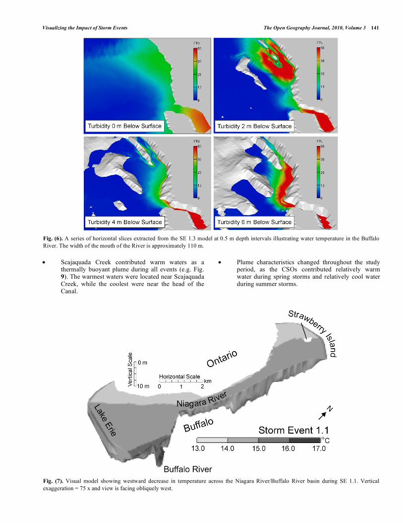
• Scajaquada Creek contributed warm waters as a thermally buoyant plume during all events (e.g. Fig. 9). The warmest waters were located near Scajaquada Creek, while the coolest were near the head of the Canal.

• Plume characteristics changed throughout the study period, as the CSOs contributed relatively warm water during spring storms and relatively cool water during summer storms.

Fig. (6). A series of horizontal slices extracted from the SE 1.3 model at 0.5 m depth intervals illustrating water temperature in the Buffalo

River. The width of the mouth of the River is approximately 110 m.

Fig. (7). Visual model showing westward decrease in temperature across the Niagara River/Buffalo River basin during SE 1.1. Vertical

exaggeration = 75 x and view is facing obliquely west.


Table 5. Registered Overflows During Storm Events

Outfall # Storm Event 1 (m3) Storm Event 2 (m3)

003 333,657.0 5,014.8

004 None 24,219.1

005 None 605.3

006 53,546.2 1,211.2

008 None 4,304.4

010 None 6,288.3

012 6,073.2 54,986.9

063 490.7 795.8

055 66,137.0 111,785.0

DISCUSSION

Prior to the study, we hypothesized that a majority of the Buffalo River sediment plume was transported into and deposited in the Canal and that even mild storm events would cause combined sewers to overflow, thus decreasing water quality in the Canal. Through the combined use of oceanic data loggers and visualizations, which enabled efficient collection, data reduction, and visual analysis of sizeable datasets, we were able to characterize water quality over a relatively large study area during varying hydrologic conditions to address these objectives. The visualizations revealed large-scale patterns (e.g. westward cooling of water temperature in the Outer Harbor and Niagara River), while discriminating local departures from these patterns (e.g. backflow of Outer Harbor water into Buffalo River during storm flows). Interpretations from these visualizations were

verified through ANOVA F-tests to indicate the statistical significance ( <0.05), if any, of differences between parameter means (i.e. temperature and turbidity) and sample depth, location, and sampling event.

The impact of the Buffalo River plume had limited impact on receiving waters, including the Niagara River, Outer Harbor, and Black Rock Canal. We believe this is probably a result of the following factors:

• The northwest-southeast oriented breakwalls are positioned in a staggered alignment (see Fig. 2C), which probably reduces wave energy and prevents outflow from the River from directly entering the lake as a coherent plume. The visualizations suggest that the plume mixes with ambient water in the Outer Harbor and settles quickly or, in under certain conditions, moves northward toward the head of the Canal (see Figs. 4, 5).

• During base flow conditions, Coriolis force likely causes the plume of the Buffalo River to veer to the north immediately after leaving the mouth of the River. Transects across the mouth invariably show a body of water that is more characteristic of water in the Outer Harbor, entering the River along the south shore, perhaps as a return flow that mimics estuarine circulation patterns. The northward veering plume leaves the Buffalo River as an overflow, interflow or bottom flow depending on density contrasts between ambient water and the outflow (i.e. temperature or turbidity).

• While the first two factors probably interacted synergistically to reduce the impact of sediment from the Buffalo River on ambient waters in the Niagara River, we believe the most important factor was the

Fig. (8). Temperature variability across the Niagara River/Buffalo River basin during BF 2. Despite a narrowed temperature range (late

summer sampling), note the band of cool temperatures along the Canadian shore and warmer temperatures nearest the Buffalo River. Vertical

exaggeration = 75 x and view is facing obliquely west.


difference in discharge between the two Rivers. Storm discharge from the Buffalo River during the period of study did not exceed 57m

3/s, while the

discharge across the head of the Niagara River during the same period averaged about 6370 m

3/s. The

difference in discharge resulted in considerable dilution of the storm discharge, which is likely enhanced by the break walls separating the Outer Harbor from Lake Erie and the Niagara River.

Except during BF2, the Buffalo River plume had minimal influence on the Canal, due to rapid settling within the River mouth. The sites nearest the Canal head (i.e. BC13, BC14, OH5, NR01) exhibited water quality characteristics closer to ambient levels found in the Niagara River than those in the Buffalo River. We believe the rapid settling of sediment is caused by dredging, which produces a channel geometry that is out of hydraulic equilibrium with the natural flow regime and reduces discharge by nearly 50%. However, Buffalo River sediment has been found in sediment cores taken at the mouth of the Niagara River [44], indicating that some sediment is transported down the Niagara River during larger storm events. There is also little evidence that wind and wave action (primarily from the southwest) redirected the Buffalo River plume into the Erie Basin Marina (see Fig. 2C). Irvine [21] deployed a continuously recording monitor (Hydrolab 4) in the mouth of the Erie Basin Marina and found that mean turbidity over the 30 week sampling period was relatively low (4 FTUs) and showed little dispersion ( = 4 FTUs). This is two magnitudes lower than those measured at one of Irvine’s monitoring sites within the mouth of the Buffalo River. Our visual models corroborate this and, as a result, the Niagara River, Black Rock Canal, and Marina are eliminated as relatively consistent sinks for Buffalo River sediments.

Although the Buffalo River had limited impact on the Canal, there is strong evidence that the Canal is affected by CSOs, which is established from continuous dataloggers positioned at outfalls [43] and the visualizations developed during this study. Three-dimensional sampling, in contrast to 1-dimensional, continuous sampling, affords the possibility of mapping the horizontal and vertical extent and monitoring the persistence of individual overflows. For example, the impact of CSO #012 (see Fig. 2B) was evident during and

after both storm events. Irvine [21] reports mean turbidity at Outfall #012 for 30 weeks was 45 FTUs ( = 85 FTUs) and that over 45% of the days between April and November were considered non-compliant with levels of dissolved oxygen (<4.0 mg/l or daily concentrations > 5.0 mg/l) near the outfall. Our visual models corroborate this; however, the visualizations indicate the effluent from #012 (the only outfall between sampling sites BC11, 12 and BC10, 9) has no impact on the upstream sample sites (BC11, 12) but does diffuse slowly downstream (e.g. mean turbidity and temperature from sites BC9, 10 were significantly ( <0.05) higher than BC 11, 12 during SE 1).

Although the impact CSOs have on water quality has been explored in depth for more than half a century, efforts to reduce overflow rates and to remediate urban water bodies affected by these overflows have just recently become the focal point of observation and analysis. In this study, the goal was to visualize the spatial and temporal variability of CSOs in Western New York and our findings indicate there is a significant first flush of particulates and thermally-enriched water. While the sampling interval was probably too large to reveal the detailed changes in overflow characteristics, prior research on the impact of CSOs on urban waterways have observed and described the essence of the first flush [46-48]. Extended periods of antecedent conditions, followed by an intense rainfall event, tend to flush relatively more material out of the systems, thus increasing the particulate and contaminant loading to the water body [46]. Although the rainstorms in our study were relatively subdued, there was an increase in sediment loading immediately following the onset of the rainfall event (relative to the second, third and fourth sampling event). Also, some effects of CSOs may have a delayed impact, such as dissolved oxygen [47-50]; the impact of oxygen depletion from a CSO on a receiving water body may outlast the overflow event [49]. Within this study, we did observe warm waters (although dissolved oxygen was collected, for this paper temperature was used as a surrogate for dissolve oxygen), especially in the Canal, lingering and affecting later sampling runs more than suspended sediments.

Most efforts to understand the impact of CSOs have characterized the first flush or the chemical, physical, and biological composition of an overflow. Frequently, the

Fig. (9). Three-dimensional visualization of temperature in the Buffalo River/Black Rock Canal basin during SE 1.1. Vertical exaggeration =

75 x and view is facing obliquely west.


impact of a CSO on water quality is measured by collecting grab samples [48] or using a data loggers positioned in or near the outfall to continuously measure the physical properties or biological/chemical composition of overflow events [21, 51]. The value of continuous data is clear, especially with regards to measuring discharge amount and timing of event, but this approach typically relies on one fixed sampling location and is therefore spatially limited. However, Even et al. [50] stressed the importance of the impact on water quality due to the “geographical dispersion” of CSOs, especially in urban areas that have a relatively high density of discharge points, such as in the Buffalo River and Black Rock Canal. Despite this interest in effluent extent, an insufficient amount of research has visualized the 3-dimensional characteristics of overflows during multiple overflow events. So in order to record the vertical and horizontal extent of CSOs and sediment plumes on receiving waters, our sampling protocol required intense field monitoring with oceanographic data loggers that could acquire multiple depth readings at each site. While predicting storm events and mobilizing a research crew was a logistical challenge, patterns derived from using this sampling design revealed the geographical dispersion of suspended sediment from various CSOs and discharge points. Thus, the application of field-intensive monitoring before, during, and after storm events to visualize plume extent is innovative and effective because:

• The spatial dimensions of an individual plume can be obtained and, over time, the nature of the plume (e.g. rate of sediment dispersal) correlated to storm intensity and distribution, stream hydrology and geomorphology, and characteristics of the sewer shed or source area (e.g. imperviousness, discharge points, time of concentration).

• Potential zones of deposition can be surmised, such that the accumulation of potentially contaminated sediments is identified. The visualizations can also guide efforts to remediate these contaminated sediment sinks or to dredge to maintain appropriate channel depths for ship passage.

• The objectives of a study or the sampling protocol can be guided by interpretations made from visualizations (thus the visual models contribute to the development of the methods). While we maintained the same sampling protocol throughout the study, the visualizations specify the need to increase the number of Canal in order to optimize the analysis of each contributing outfall. Many visualization software packages can analyze and report the uncertainty associated with any distribution of sampling sites, which can also aid the design of an appropriate sample protocol.

Visualizations can certainly elicit interactions of various physio-chemical processes, but they are limited in the ability to discriminate among the hydrodynamic processes. The visual models are descriptors of the physical environmental, which can lead to multiple interpretations of the hydrodynamics extracted from any visualization. For example, we concluded, based on the visualizations and data analysis, that only a relatively small amount of suspended sediment from the Buffalo River actually entered the Outer

Harbor and Niagara River during the sampling events. There is evidence in the visualizations that support these hypotheses, but they do not necessarily indicate causation. To further discriminate between multiple causes, visualizations could be generated alongside current meters that measure flow characteristics or compared with predictions from numerical models. In addition, the effectiveness of visualizations in describing and analyzing the impact of CSOs on water quality will depend on the characteristics of sampling events. In this study, suspended sediment from the Buffalo River did not enter the Canal during the storm events that we sampled, but did enter during a baseflow event. Whether that event was an anomaly or there was a complex mechanism that caused sediment to be mobilized during baseflow conditions can only be determined by sampling a wider range of storm and baseflow events (e.g. Lee and Bang [48] collected grab samples during 34 storm events; this produced a more reliable summation of the overflows but is also logistically simpler than this study).

Visualizations of transient events, such as a CSO, can contribute to remediation planning as well. The majority of sediment leaving the mouth of the Buffalo River, for example, settled quickly within an area 150 m (east to west) x 300 m (south to north) from the River mouth (i.e. sediments deposited east of the OH1 to OH4 transect on Fig. 2C). The impact small tributaries and discharge points have on water quality can be detected with visualizations, if using a proper sample interval and distribution, which then guides remediation efforts to specific areas for sediment coring and analysis, dredging and contaminant remediation, or habitat rehabilitation.

CONCLUSIONS

Combining intense field monitoring and visual model development produced a snapshot perspective of the impact CSOs have on water quality, as well sediment mobilization due to storm events, in Northeastern Lake Erie. While the fate of suspended sediment from the Buffalo River requires more attention, our visualizations suggest that most of the sediment settles quickly, but also that relatively minor rainfall events can initiate overflows and sediment mobilization. CSO discharges, in particular, increase parameter variability, which clearly has a detrimental impact on the quality of the river system. The mergence of graphical and visual analysis of spatial and temporal data highlighted water quality trends throughout the study area that would otherwise be difficult using remote sensing techniques or continuously recording data loggers (e.g. westward cooling of water temperature in the Outer Harbor and Niagara River and the backflow of Outer Harbor water into Buffalo River during storm flows). Although EVS-Pro was unable to generate a visualization of parameter variability in both the Canal and the Niagara River, we believe the visualizations efficiently and effectively supported our objectives of analyzing general trends and mapping the impact storm events have on water quality. Generating 2- and 3-dimensional visualizations based on intense data acquisition can reveal water quality trends in large water bodies, directly supporting management or remediation efforts or understanding capture system responses to dynamic marine or lacustrine conditions.


ACKNOWLEDGEMENTS

The authors are grateful for the statistical support from Dr. Thomas Snabb. The content and structure of this manuscript was greatly improved by three anonymous reviewers. The authors would also like to thank the Buffalo State College Great Lakes Research Center, the Buffalo Sewer Authority, Malcom Pirnie, and URS Greiner for their logistical and financial support. The authors also thank Dr. Kim Irvine, whose network of data loggers during this project provided valuable corroboration for the visual models.

REFERENCES

[1] United States Environmental Protection Agency (USEPA).

Combined–sewer overflow policy. Fed Reg 1994; 59(75): 18688. [2] Lijklema L,Tyson JM. Urban water quality: interactions between

sewers, treatment plants, and receiving waters. Water Sci Technol 1993; 27(5): 29-33.

[3] Field R, Struzeski EJ. Management and control of combined-sewer overflows. J Water Pollut Control Fed 1972; 44(7): 1393-1415.

[4] Diaz-Fierros T, Puerta J, Suarez JF, Diaz-Fierros V. Contaminant loads of CSOs at the wastewater treatment plant of a city in NW

Spain. Urban Water 2002; 4: 291-99. [5] Sakrabani R, Vollertsen J, Ashley RM, Hvitved-Jacobsen T.

Biodegradability of organic matter associated with sewer sediments during first flush. Sci Total Environ 2009; 407: 2989-95.

[6] Lick W, Xu YJ, McNeil J. Resuspension properties of sediments from the Fox, Saginaw, and Buffalo Rivers. J Great Lakes Res

1995; 21: 257-74. [7] Pettibone GW, Irvine KN, Monahan KM. Impact of ship passage

on bacteria levels and suspended sediment characteristics in the Buffalo River, New York. Water Resour Res 1996; 30(10): 2517-

21. [8] Irvine KN, Pettibone GW. Planning level evaluation of densities of

indicator bacteria in a mixed land use watershed. Environ Technol 1996; 17: 1-12.

[9] Rosa F. Sedimentation and sediment resuspension in Lake Ontario. J Great Lakes Res 1985; 11: 13-25.

[10] Lou J, Schwab DJ, Beletsky D, Hawle N. A model of sediment resuspension and transport dynamics in southern Lake Michigan. J

Geophys Res 2000; 105: 6591-610. [11] Eadie BJ, Schwab DJ, Johengen TH, et al. Particle transport,

nutrient cycling, and algal community structure associated with a major winter-spring sediment resuspension event in southern Lake

Michigan. J Great Lakes Res 2002; 28: 324-37. [12] Halfman JD, Dittman DE, Owens RW, Etherington MD. Storm-

induced redistribution of deepwater sediments in Lake Ontario. J Great Lakes Res 2006; 32: 348-60.

[13] Schwab DJ, Eadie BJ, Assel RA, Roebber, PJ. Climatology of large sediment resupsension events in southern Lake Michigan. J Great

Lakes Res 2006; 32: 50-62. [14] Irvine KN, Droppo IG, Murphy TP, Lawson, A. Sediment

resuspension and dissolved oxygen levels associated with ship traffic: implications for habitat remediation. Water Qual Res J Can

1997; 32: 421-37. [15] Binding CE, Bowers DG, Mitchelson-Jacob EG. Estimating

suspended sediment concentrations from ocean color measurements in moderately turbid waters; the impact of variable particle

scattering properties. Remote Sens Environ 2005; 94(3): 373-83. [16] MacIntyre S, Flynn KM, Jellison R, Romero, JR. Boundary mixing

and nutrient flux in Mono Lake, CA. Limnol Oceanogr1999; 44: 512-29.

[17] MacIntyre S, Jellison R. Nutrient fluxes from upwelling and enhanced turbulence at the top of the pycnocline in Mono Lake,

CA. Hydrobiologia 2001; 466:13-29. [18] MacIntyre S, Romero JR, Kling GW. Spatial-temporal variability

in mixed layer deepening and lateral advection in an embayment of Lake Victoria, East Africa. Limnol Oceanogr 2002; 47: 656-71.

[19] Pineda J, DiBacco C, Starczak, V. Barnacle larvae in ice: survival, reproduction, and time to post settlement metamorphosis. Limnol

Oceanogr 2005; 50(5): 1520-28.

[20] Sargent GH. Water pollution investigation: Buffalo River. United

States Environmental Protection Agency (EPA) Report, EPA- 905/9-74-010 1975.

[21] Irvine KN. Continuous monitoring of conventional parameters in the Buffalo River, Harbor, and Black Rock Canal - A preliminary

assessment. Report to URS Griener Woodward Clyde, Long Term Control Plan Project 2001; p. 84.

[22] Fraser G, Freidhoff J, Goehle M, Napieralski J. Three-dimensional structure of the water mass in Eastern Lake Erie as revealed by

intensive CTD monitoring and three-dimensional visualization. Great Lakes Res Rev 2001; 5(2): 25-30.

[23] Kim D, Chung C, Sun C, Bang E. Site assessment and evaluation of spatial earthquake ground motion of Kyeongju. Soil Dyn

Earthquake Eng 2002; 22: 371-87. [24] Grunwald S, Barak P, McSweeney K, Lowery B. Soil landscape

models at different scales portrayed in virtual reality modeling language. Soil Sci 2000; 165(08): 598-615.

[25] Irvine KN, Pettibone GW. Dynamics of indicator bacteria populations in sediment and water near a combined sewer outfall.

Environ Technol 1993; 14: 531-42. [26] New York State Department of Environmental Conservation

(NYSDEC). Buffalo River Remedial Action Plan. Report to the IJC 1989.

[27] Owens DW, Pittman WL, Wulforst JP, Hanna WE. Soil Survey of Erie County: U.S. Department of Agriculture, Soil Conservation

Service, Washington 1986; p. 384. [28] Gailani J, Lick W, Ziegler K, Endicott D. Development and

calibration of a fine-grained sediment transport model for the Buffalo River. J Great Lakes Res 1996; 22(3): 765-78.

[29] Meredith DD, Rumer RR. Sediment dynamics in the Buffalo River. Report. Department of Civil Engineering, SUNY at Buffalo 1987;

p. 171. [30] Raggio G, Jirka GH. Fine contaminated sediment

erosion/deposition in the Buffalo River, New York. In Proceedings National Conference on Hydraulic Engineering, Colorado Springs,

Co. American Society of Civil Engineers 1988; 850-6. [31] Wen J, Jirka GH, Raggio G. Linked sediment/contaminant

transport model for rivers with application to the Buffalo River. J Great Lakes Res 1994; 20(4): 671-82.

[32] Irvine KN, Loganathan BG, Pratt EJ, Sikka, HC. Calibration of PCSWMM to estimate metals, PCBs and HCB in CSOs from an

industrial sewershed, Buffalo, N.Y. In: James W, Ed. New techniques for modeling the management of storm water quality

impacts. Boca Raton, FL: Lewis Publishers Inc 1993; pp. 215-42. [33] Loganathan BG, Irvine KN, Kannan K, Pragatheeswaran V,

Sajwan KS. Distribution of selected PCB congeners in the Babcock street sewer district: a multimedia approach to identify PCB

sources in combined sewer overflows (CSOs) discharging to the Buffalo River, New York. Arch Environ Contam Toxicol 1997; 33:

130-40. [34] Raggio G, Jirka G, Pacenka S. Modeling and field studies of

sediment transport in the Buffalo River, Erie County, New York. Technical report. Center for Environmental Research. New York

State Water Resour Res institute, Cornell University 1988; p. 77. [35] Wang PF, Martin JL. Temperature and conductivity modeling for

the Buffalo River. J Great Lakes Res 1991; 17(4): 495-503. [36] Singer JK, Irvine KN, Snyder R, Shero B, Manley P, McLaren P.

Fish and Wildlife Habitat Assessment of the Buffalo River Area of Concern and Watershed. Report to the U.S. EPA, Great Lakes

National Program Office, D.C. 1995 [37] Salomons W, de Rooij NM, Kerdijk H, Bril J. Sediments as a

source for contaminants? Hydrobiologia 1987; 149: 13-30. [38] Litten S. Niagara area sediments. Technical report. New York State

Department of Environmental Conservation 1987. [39] Crissman RD, Chiu C, Yu W, Mizumura K, Corbu I. Uncertainties

in flow modeling and forecasting for Niagara River. J Hydraul Eng 1993; 119(11): 1231-49.

[40] Atkinson JF, Lin G, Joshi M. Physical model of Niagara River discharge. J Great Lakes Res 1994; 20(3): 583-9.

[41] Blair SH, Atkinson, JF. Effect of flow diversions on contaminant transport modeling in the Niagara River. J Great Lakes Res 1993;

19(1): 83-95. [42] Hayashida T, Atkinson JF, DePinto JV, Rumer RR. A numerical

study of the Niagara River discharge near-shore flow field in Lake Ontario. J Great Lakes Res 1999; 25(4): 897-909.


[43] Irvine KN. Preliminary assessment of hydrolab data for the grant

street site, Scajaquada creek - a preliminary assessment. Report to Malcolm Pirnie, Inc., Long Term Control Plan Project, 2001; p. 36.

[44] United States Environmental Protection Agency (USEPA). Niagara River Area of Concern. Technical Report 1999.

[45] Isaaks ED, Srivaslava RM. An introduction to applied geostatistics. USA: Oxford University Press 1989; p. 592.

[46] Gupta K, Saul AD. Specific relationships for the first flush load in combined sewer flows. Water Res1996; 30: 1244-52.

[47] Krebs P, Holzer P, Huisman JL, Rauch, W. First flush of dissolved compounds. Water Sci Technol 1999; 39: 55-62.

[48] Lee JH, Bang, KW. Characterization of urban storm water runoff.

Water Res 2000; 34: 1773-80. [49] Hvitved-Jacobsen T. The impact of combined sewer overflows on

the dissolved oxygen concentration of a river. Water Res 1982; 16: 1099-105.

[50] Even S, Mouchel J-M, Servais P, et al. Modeling the impacts of combined sewer overflows in the river Seine water quality. Sci

Total Environ 2007; 375: 140-51. [51] Lawler DM, Petts GE, Foster IDL, Harper S. Turbidity dynamics

during spring storm events in an urban headwater river system: the upper tame, West Midlands, UK. Sci Total Environ 2006; 360:

109-26.

Received: November 3, 2009 Revised: February 16, 2010 Accepted: July 1, 2010

© Napieralski and Fraser; Licensee Bentham Open.

This is an open access article licensed under the terms of the Creative Commons Attribution Non-Commercial License (http://creativecommons.org/licenses/by-

nc/3.0/) which permits unrestricted, non-commercial use, distribution and reproduction in any medium, provided the work is properly cited.

open access visualizing the impact of storm …jnapiera/cv_files/... · river, which drains into...

Documents