#open data butlerschofield apr 2010 liberal media...

#Open data data <- read.csv("/Users/mdweaver/Desktop/ButlerSchofield_APR_2010_liberal_media_bias_data.csv") #Create variables used in regressions data$mcl_mcend <- 0 data$mcl_mcend[data$mccain == 1 & data$endorse == 1] <- 1 data$mcl_obend <- 0 data$mcl_obend[data$mccain == 1 & data$endorse == 5] <- 1 data$obl_mcend <- 0 data$obl_mcend[data$mccain == 0 & data$endorse == 1] <- 1 data$differ <- 0 data$differ[data$mcl_obend == 1 | data$obl_mcend == 1] <- 1 #Create observations to be used for estimating marginal effects for control variables library(gmodels) CrossTable(data$mccain, data$interest_in_letter, prop.c=FALSE, prop.t=FALSE, prop.chisq=FALSE, chisq=TRUE)

Cell Contents|-------------------------|| N || N / Row Total ||-------------------------|

Total Observations in Table: 100

| data$interest_in_letter data$mccain | 0 | 1 | Row Total | -------------|-----------|-----------|-----------| 0 | 41 | 10 | 51 | | 0.804 | 0.196 | 0.510 | -------------|-----------|-----------|-----------| 1 | 33 | 16 | 49 | | 0.673 | 0.327 | 0.490 | -------------|-----------|-----------|-----------|Column Total | 74 | 26 | 100 | -------------|-----------|-----------|-----------|

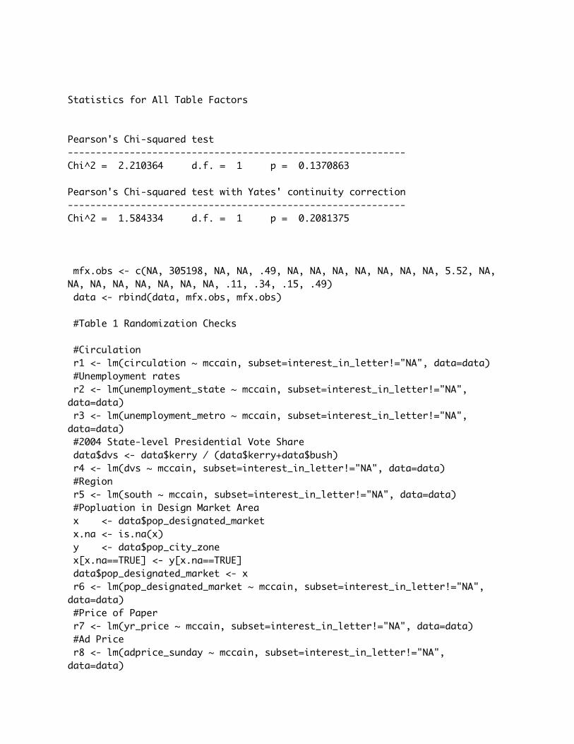
Statistics for All Table Factors

Pearson's Chi-squared test ------------------------------------------------------------Chi^2 = 2.210364 d.f. = 1 p = 0.1370863

Pearson's Chi-squared test with Yates' continuity correction ------------------------------------------------------------Chi^2 = 1.584334 d.f. = 1 p = 0.2081375

mfx.obs <- c(NA, 305198, NA, NA, .49, NA, NA, NA, NA, NA, NA, NA, 5.52, NA, NA, NA, NA, NA, NA, NA, NA, .11, .34, .15, .49) data <- rbind(data, mfx.obs, mfx.obs) #Table 1 Randomization Checks #Circulation r1 <- lm(circulation ~ mccain, subset=interest_in_letter!="NA", data=data) #Unemployment rates r2 <- lm(unemployment_state ~ mccain, subset=interest_in_letter!="NA", data=data) r3 <- lm(unemployment_metro ~ mccain, subset=interest_in_letter!="NA", data=data) #2004 State-level Presidential Vote Share data$dvs <- data$kerry / (data$kerry+data$bush) r4 <- lm(dvs ~ mccain, subset=interest_in_letter!="NA", data=data) #Region r5 <- lm(south ~ mccain, subset=interest_in_letter!="NA", data=data) #Popluation in Design Market Area x <- data$pop_designated_market x.na <- is.na(x) y <- data$pop_city_zone x[x.na==TRUE] <- y[x.na==TRUE] data$pop_designated_market <- x r6 <- lm(pop_designated_market ~ mccain, subset=interest_in_letter!="NA", data=data) #Price of Paper r7 <- lm(yr_price ~ mccain, subset=interest_in_letter!="NA", data=data) #Ad Price r8 <- lm(adprice_sunday ~ mccain, subset=interest_in_letter!="NA", data=data)

#Table 2 #probit 1 library(Zelig)Loading required package: MASSLoading required package: boot## ## Zelig (Version 3.4-5, built: 2009-03-13)## Please refer to http://gking.harvard.edu/zelig for full## documentation or help.zelig() for help with commands and## models supported by Zelig.##

## Zelig project citations:## Kosuke Imai, Gary King, and Olivia Lau. (2009).## ``Zelig: Everyone's Statistical Software,''## http://gking.harvard.edu/zelig.## and## Kosuke Imai, Gary King, and Olivia Lau. (2008).## ``Toward A Common Framework for Statistical Analysis## and Development,'' Journal of Computational and## Graphical Statistics, Vol. 17, No. 4 (December)## pp. 892-913.

## To cite individual Zelig models, please use the citation format printed with## each model run and in the documentation.## probit.1 <- zelig(interest_in_letter ~ mccain, model = "probit" , data=data)How to cite this model in Zelig:Kosuke Imai, Gary King, and Oliva Lau. 2007. "probit: Probit Regression for Dichotomous Dependent Variables" in Kosuke Imai, Gary King, and Olivia Lau, "Zelig: Everyone's Statistical Software," http://gking.harvard.edu/zelig summary(probit.1)

Call:zelig(formula = interest_in_letter ~ mccain, model = "probit", data = data)

Deviance Residuals: Min 1Q Median 3Q Max -0.889 -0.889 -0.661 1.496 1.805

Coefficients: Estimate Std. Error z value Pr(|z|)

http://gking.harvard.edu/zelig






(Intercept) -0.856 0.201 -4.26 2.1e-05 ***mccain 0.406 0.274 1.48 0.14 ---Signif. codes: 0 ‘***’ 0.001 ‘**’ 0.01 ‘*’ 0.05 ‘.’ 0.1 ‘ ’ 1

(Dispersion parameter for binomial family taken to be 1)

Null deviance: 114.61 on 99 degrees of freedomResidual deviance: 112.39 on 98 degrees of freedomAIC: 116.4

Number of Fisher Scoring iterations: 4

#simulated marginal effect of mccain letter # Marginal effects obtained in R through Zelig, which uses simulations to estimate the size of the marginal effect. Stata calculates the effect directly. See the documentation on the Zelig package to learn more about this. p1.out1 <- setx(probit.1, mccain=0) p1.out2 <- setx(probit.1, mccain=1) s.out1 <- sim(probit.1, num=c(50000,100), x = p1.out1, x1=p1.out2) summary(s.out1)

Model: probit Number of simulations: 50000

Values of X (Intercept) mccain8 1 0

Values of X1 (Intercept) mccain8 1 1

Expected Values: E(Y|X) mean sd 2.5% 97.5%1 0.2006 0.05545 0.1065 0.3225

Predicted Values: Y|X 0 11 0.801 0.1989

First Differences in Expected Values: E(Y|X1)-E(Y|X) mean sd 2.5% 97.5%1 0.1285 0.08615 -0.04118 0.2971

Risk Ratios: P(Y=1|X1)/P(Y=1|X) mean sd 2.5% 97.5%1 1.778 0.6554 0.8556 3.38 #probit 2 probit.2 <- zelig(interest_in_letter ~ mccain + circulation + unemployment_metro, model = "probit" , data=data)How to cite this model in Zelig:Kosuke Imai, Gary King, and Oliva Lau. 2007. "probit: Probit Regression for Dichotomous Dependent Variables" in Kosuke Imai, Gary King, and Olivia Lau, "Zelig: Everyone's Statistical Software," http://gking.harvard.edu/zelig summary(probit.2)

Call:zelig(formula = interest_in_letter ~ mccain + circulation + unemployment_metro, model = "probit", data = data)


Coefficients: Estimate Std. Error z value Pr(|z|) (Intercept) -2.25e-01 7.45e-01 -0.30 0.762 mccain 5.84e-01 2.92e-01 2.00 0.045 *circulation -2.81e-06 1.28e-06 -2.20 0.028 *unemployment_metro -9.13e-03 1.23e-01 -0.07 0.941 ---Signif. codes: 0 ‘***’ 0.001 ‘**’ 0.01 ‘*’ 0.05 ‘.’ 0.1 ‘ ’ 1




#simulated marginal effect of mccain letter p2.out1 <- setx(probit.2, mccain=0, unemployment_metro = 5.52, circulation = 305198) p2.out2 <- setx(probit.2, mccain=1, unemployment_metro = 5.52, circulation = 305198)



s.out2 <- sim(probit.2, num=c(50000,100), x=p2.out1, x1=p2.out2) summary(s.out2)


Values of X (Intercept) mccain circulation unemployment_metro8 1 0 305198 5.52

Values of X1 (Intercept) mccain circulation unemployment_metro8 1 1 305198 5.52



First Differences in Expected Values: E(Y|X1)-E(Y|X) mean sd 2.5% 97.5%1 0.1596 0.08009 0.003904 0.3193

Risk Ratios: P(Y=1|X1)/P(Y=1|X) mean sd 2.5% 97.5%1 2.518 1.228 1.018 5.629 #simulated marginal effect of 1 sd change in circulation p2.out3 <- setx(probit.2, mccain=.49, unemployment_metro = 5.52, circulation = 305198) p2.out4 <- setx(probit.2, mccain=.49, unemployment_metro = 5.52, circulation = 649366) s.out3 <- sim(probit.2, num=c(50000,100), x=p2.out3, x1=p2.out4) summary(s.out3)


Values of X (Intercept) mccain circulation unemployment_metro8 1 0.49 305198 5.52

Values of X1

(Intercept) mccain circulation unemployment_metro8 1 0.49 649366 5.52



First Differences in Expected Values: E(Y|X1)-E(Y|X) mean sd 2.5% 97.5%1 -0.1453 0.04503 -0.2185 -0.03551

Risk Ratios: P(Y=1|X1)/P(Y=1|X) mean sd 2.5% 97.5%1 0.2474 0.2289 0.01273 0.8625 #simulated marginal effects of 1 sd change in metro-area unemployment p2.out5 <- setx(probit.2, mccain=.49, unemployment_metro = 5.52, circulation = 305198) p2.out6 <- setx(probit.2, mccain=.49, unemployment_metro = 6.65, circulation = 305198) s.out4 <- sim(probit.2, num=c(50000,100), x=p2.out5, x1=p2.out6) summary(s.out4)


Values of X (Intercept) mccain circulation unemployment_metro8 1 0.49 305198 5.52

Values of X1 (Intercept) mccain circulation unemployment_metro8 1 0.49 305198 6.65



First Differences in Expected Values: E(Y|X1)-E(Y|X) mean sd 2.5% 97.5%1 -0.0007817 0.0388 -0.07218 0.08122

Risk Ratios: P(Y=1|X1)/P(Y=1|X) mean sd 2.5% 97.5%1 0.998 0.1961 0.6493 1.414 #Table 3 data.3 <- subset(data, data$endorse==1 | data$endorse==5) probit.3 <- zelig(interest_in_letter ~ mcl_mcend + mcl_obend + obl_mcend, model = "probit" , data=data.3)How to cite this model in Zelig:Kosuke Imai, Gary King, and Oliva Lau. 2007. "probit: Probit Regression for Dichotomous Dependent Variables" in Kosuke Imai, Gary King, and Olivia Lau, "Zelig: Everyone's Statistical Software," http://gking.harvard.edu/zelig summary(probit.3)

Call:zelig(formula = interest_in_letter ~ mcl_mcend + mcl_obend + obl_mcend, model = "probit", data = data.3)


Coefficients: Estimate Std. Error z value Pr(|z|) (Intercept) -1.020 0.298 -3.42 0.00063 ***mcl_mcend 0.415 0.502 0.83 0.40817 mcl_obend 0.562 0.373 1.51 0.13146 obl_mcend 0.767 0.443 1.73 0.08349 . ---Signif. codes: 0 ‘***’ 0.001 ‘**’ 0.01 ‘*’ 0.05 ‘.’ 0.1 ‘ ’ 1




#simulated marginal effect of endorsed McCain/received McCain letter p3.out1 <- setx(probit.3, mcl_mcend = 0, mcl_obend = .34, obl_mcend = .15)



p3.out2 <- setx(probit.3, mcl_mcend = 1, mcl_obend = .34, obl_mcend = .15) s.out5 <- sim(probit.3, num=c(50000,100), x=p3.out1, x1=p3.out2) summary(s.out5)


Values of X (Intercept) mcl_mcend mcl_obend obl_mcend8 1 0 0.34 0.15

Values of X1 (Intercept) mcl_mcend mcl_obend obl_mcend8 1 1 0.34 0.15




Risk Ratios: P(Y=1|X1)/P(Y=1|X) mean sd 2.5% 97.5%1 1.753 0.8923 0.4619 3.887 #simulated marginal effect of endorsed Obama/received McCain letter p3.out3 <- setx(probit.3, mcl_mcend = .11, mcl_obend = 0, obl_mcend = .15) p3.out4 <- setx(probit.3, mcl_mcend = .11, mcl_obend = 1, obl_mcend = .15) s.out6 <- sim(probit.3, num=c(50000,100), x=p3.out3, x1=p3.out4) summary(s.out6)


Values of X (Intercept) mcl_mcend mcl_obend obl_mcend8 1 0.11 0 0.15

Values of X1 (Intercept) mcl_mcend mcl_obend obl_mcend

8 1 0.11 1 0.15




Risk Ratios: P(Y=1|X1)/P(Y=1|X) mean sd 2.5% 97.5%1 2.175 1.057 0.8139 4.823 #simulated marginal effect of endorsed McCain/received Obama letter p3.out5 <- setx(probit.3, mcl_mcend = .11, mcl_obend = .34, obl_mcend = 0) p3.out6 <- setx(probit.3, mcl_mcend = .11, mcl_obend = .34, obl_mcend = 1) s.out7 <- sim(probit.3, num=c(50000,100), x=p3.out5, x1=p3.out6) summary(s.out7)


Values of X (Intercept) mcl_mcend mcl_obend obl_mcend8 1 0.11 0.34 0

Values of X1 (Intercept) mcl_mcend mcl_obend obl_mcend8 1 0.11 0.34 1




Risk Ratios: P(Y=1|X1)/P(Y=1|X) mean sd 2.5% 97.5%1 2.419 1.041 0.8836 4.9 #Probit 4 probit.4 <- zelig(interest_in_letter ~ mcl_mcend + mcl_obend + obl_mcend + circulation + unemployment_metro, model = "probit" , data=data.3)How to cite this model in Zelig:Kosuke Imai, Gary King, and Oliva Lau. 2007. "probit: Probit Regression for Dichotomous Dependent Variables" in Kosuke Imai, Gary King, and Olivia Lau, "Zelig: Everyone's Statistical Software," http://gking.harvard.edu/zelig summary(probit.4)

Call:zelig(formula = interest_in_letter ~ mcl_mcend + mcl_obend + obl_mcend + circulation + unemployment_metro, model = "probit", data = data.3)


Coefficients: Estimate Std. Error z value Pr(|z|) (Intercept) -2.19e-01 8.47e-01 -0.26 0.796 mcl_mcend 3.80e-01 5.37e-01 0.71 0.478 mcl_obend 6.69e-01 3.88e-01 1.72 0.085 .obl_mcend 6.07e-01 4.56e-01 1.33 0.183 circulation -2.35e-06 1.23e-06 -1.90 0.057 .unemployment_metro -4.35e-02 1.30e-01 -0.33 0.739 ---Signif. codes: 0 ‘***’ 0.001 ‘**’ 0.01 ‘*’ 0.05 ‘.’ 0.1 ‘ ’ 1




#simulated marginal effect of endorsed McCain/received McCain letter



p4.out1 <- setx(probit.4, mcl_mcend = 0, mcl_obend = .34, obl_mcend = .15, circulation=305198, unemployment_metro=5.52) p4.out2 <- setx(probit.4, mcl_mcend = 1, mcl_obend = .34, obl_mcend = .15, circulation=305198, unemployment_metro=5.52) s.out8 <- sim(probit.4, num=c(50000,100), x=p4.out1, x1=p4.out2) summary(s.out8)


Values of X (Intercept) mcl_mcend mcl_obend obl_mcend circulation unemployment_metro8 1 0 0.34 0.15 305198 5.52

Values of X1 (Intercept) mcl_mcend mcl_obend obl_mcend circulation unemployment_metro8 1 1 0.34 0.15 305198 5.52




Risk Ratios: P(Y=1|X1)/P(Y=1|X) mean sd 2.5% 97.5%1 1.839 1.139 0.3584 4.632 #simulated marginal effect of endorsed Obama/received McCain letter p4.out3 <- setx(probit.4, mcl_mcend = .11, mcl_obend = 0, obl_mcend = .15, circulation=305198, unemployment_metro=5.52) p4.out4 <- setx(probit.4, mcl_mcend = .11, mcl_obend = 1, obl_mcend = .15, circulation=305198, unemployment_metro=5.52) s.out9 <- sim(probit.4, num=c(50000,100), x=p4.out3, x1=p4.out4) summary(s.out9)


Values of X

(Intercept) mcl_mcend mcl_obend obl_mcend circulation unemployment_metro8 1 0.11 0 0.15 305198 5.52

Values of X1 (Intercept) mcl_mcend mcl_obend obl_mcend circulation unemployment_metro8 1 0.11 1 0.15 305198 5.52




Risk Ratios: P(Y=1|X1)/P(Y=1|X) mean sd 2.5% 97.5%1 2.75 1.598 0.8866 6.831 #simulated marginal effect of endorsed McCain/received Obama letter p4.out5 <- setx(probit.4, mcl_mcend = .11, mcl_obend = .34, obl_mcend = 0, circulation=305198, unemployment_metro=5.52) p4.out6 <- setx(probit.4, mcl_mcend = .11, mcl_obend = .34, obl_mcend = 1, circulation=305198, unemployment_metro=5.52) s.out10 <- sim(probit.4, num=c(50000,100), x=p4.out5, x1=p4.out6) summary(s.out10)


Values of X (Intercept) mcl_mcend mcl_obend obl_mcend circulation unemployment_metro8 1 0.11 0.34 0 305198 5.52

Values of X1 (Intercept) mcl_mcend mcl_obend obl_mcend circulation unemployment_metro8 1 0.11 0.34 1 305198 5.52




Risk Ratios: P(Y=1|X1)/P(Y=1|X) mean sd 2.5% 97.5%1 2.297 1.198 0.6694 5.228 #simulated marginal effect of 1 sd increase in circulation p4.out7 <- setx(probit.4, mcl_mcend = .11, mcl_obend = .34, obl_mcend = .15, circulation=305198, unemployment_metro=5.52) p4.out8 <- setx(probit.4, mcl_mcend = .11, mcl_obend = .34, obl_mcend = .15, circulation=649366, unemployment_metro=5.52) s.out11 <- sim(probit.4, num=c(50000,100), x=p4.out7, x1=p4.out8) summary(s.out11)


Values of X (Intercept) mcl_mcend mcl_obend obl_mcend circulation unemployment_metro8 1 0.11 0.34 0.15 305198 5.52

Values of X1 (Intercept) mcl_mcend mcl_obend obl_mcend circulation unemployment_metro8 1 0.11 0.34 0.15 649366 5.52




Risk Ratios: P(Y=1|X1)/P(Y=1|X) mean sd 2.5% 97.5%1 0.3259 0.2684 0.02423 1.027

#simulated marginal effect of 1 sd increase in metro unemploy p4.out9 <- setx(probit.4, mcl_mcend = .11, mcl_obend = .34, obl_mcend = .15, circulation=305198, unemployment_metro=5.52) p4.out10 <- setx(probit.4, mcl_mcend = .11, mcl_obend = .34, obl_mcend = .15, circulation=305198, unemployment_metro=6.65) s.out12 <- sim(probit.4, num=c(50000,100), x=p4.out9, x1=p4.out10) summary(s.out12)


Values of X (Intercept) mcl_mcend mcl_obend obl_mcend circulation unemployment_metro8 1 0.11 0.34 0.15 305198 5.52

Values of X1 (Intercept) mcl_mcend mcl_obend obl_mcend circulation unemployment_metro8 1 0.11 0.34 0.15 305198 6.65




Risk Ratios: P(Y=1|X1)/P(Y=1|X) mean sd 2.5% 97.5%1 0.9467 0.1974 0.5992 1.37 #Table 4 probit.5 <- zelig(interest_in_letter ~ differ, model = "probit", data=data.3)How to cite this model in Zelig:Kosuke Imai, Gary King, and Oliva Lau. 2007. "probit: Probit Regression for Dichotomous Dependent Variables" in Kosuke Imai, Gary King, and Olivia Lau, "Zelig: Everyone's Statistical Software," http://gking.harvard.edu/zelig summary(probit.5)

Call:



zelig(formula = interest_in_letter ~ differ, model = "probit", data = data.3)


Coefficients: Estimate Std. Error z value Pr(|z|) (Intercept) -0.881 0.238 -3.70 0.00021 ***differ 0.487 0.301 1.62 0.10531 ---Signif. codes: 0 ‘***’ 0.001 ‘**’ 0.01 ‘*’ 0.05 ‘.’ 0.1 ‘ ’ 1




#simulated marginal effect of letter differ from endorsement p5.out1 <- setx(probit.5, differ=0) p5.out2 <- setx(probit.5, differ=1) s.out13 <- sim(probit.5, num=c(50000,100), x=p5.out1, x1=p5.out2) summary(s.out13)


Values of X (Intercept) differ8 1 0

Values of X1 (Intercept) differ8 1 1


Predicted Values: Y|X 0 1

1 0.805 0.1950


Risk Ratios: P(Y=1|X1)/P(Y=1|X) mean sd 2.5% 97.5%1 2.008 0.8745 0.8787 4.197 #probit 6 #The probit coefficients and standard errors for column 2 of Table 4 published in the paper are misreported. The coefficients should have been: #Variable Coef. SE #Difference: .53 .31 #Circulation: -.23 .12 #Unemployment: -.07 .13 #The primary variable of interest - 'Difference' - is essentially correct (it was reported as 0.54 in the paper), and the predicted probability is correctly reported. probit.6 <- zelig(interest_in_letter ~ differ + circulation + unemployment_metro, model = "probit", data=data.3)How to cite this model in Zelig:Kosuke Imai, Gary King, and Oliva Lau. 2007. "probit: Probit Regression for Dichotomous Dependent Variables" in Kosuke Imai, Gary King, and Olivia Lau, "Zelig: Everyone's Statistical Software," http://gking.harvard.edu/zelig summary(probit.6)

Call:zelig(formula = interest_in_letter ~ differ + circulation + unemployment_metro, model = "probit", data = data.3)


Coefficients: Estimate Std. Error z value Pr(|z|) (Intercept) 1.95e-02 7.65e-01 0.03 0.980 differ 5.26e-01 3.12e-01 1.69 0.091 .circulation -2.29e-06 1.19e-06 -1.93 0.054 .unemployment_metro -6.65e-02 1.26e-01 -0.53 0.598 ---



Signif. codes: 0 ‘***’ 0.001 ‘**’ 0.01 ‘*’ 0.05 ‘.’ 0.1 ‘ ’ 1




#simulated marginal effect of letter differ from endorsement p6.out1 <- setx(probit.6, differ=0, unemployment_metro = 5.52, circulation = 305198) p6.out2 <- setx(probit.6, differ=1, unemployment_metro = 5.52, circulation = 305198) s.out14 <- sim(probit.6, num=c(50000,100), x=p6.out1, x1=p6.out2) summary(s.out14)


Values of X (Intercept) differ circulation unemployment_metro8 1 0 305198 5.52

Values of X1 (Intercept) differ circulation unemployment_metro8 1 1 305198 5.52




Risk Ratios: P(Y=1|X1)/P(Y=1|X) mean sd 2.5% 97.5%1 2.296 1.163 0.8978 5.236

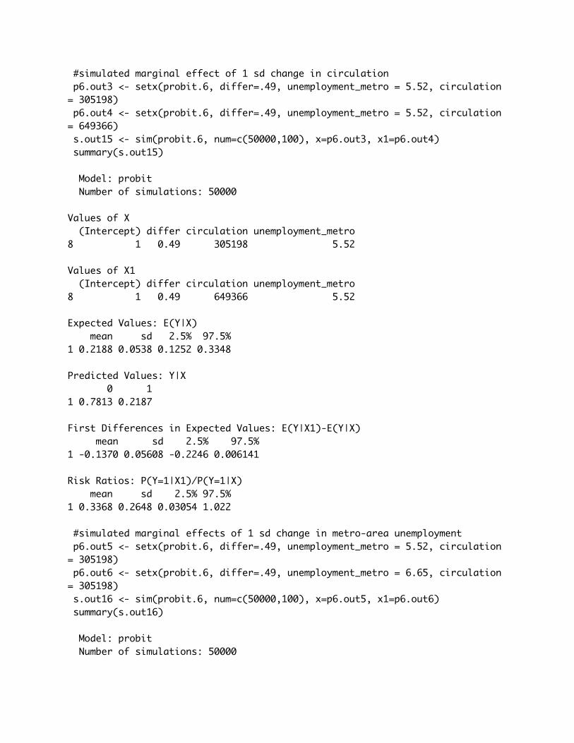
#simulated marginal effect of 1 sd change in circulation p6.out3 <- setx(probit.6, differ=.49, unemployment_metro = 5.52, circulation = 305198) p6.out4 <- setx(probit.6, differ=.49, unemployment_metro = 5.52, circulation = 649366) s.out15 <- sim(probit.6, num=c(50000,100), x=p6.out3, x1=p6.out4) summary(s.out15)


Values of X (Intercept) differ circulation unemployment_metro8 1 0.49 305198 5.52

Values of X1 (Intercept) differ circulation unemployment_metro8 1 0.49 649366 5.52




Risk Ratios: P(Y=1|X1)/P(Y=1|X) mean sd 2.5% 97.5%1 0.3368 0.2648 0.03054 1.022 #simulated marginal effects of 1 sd change in metro-area unemployment p6.out5 <- setx(probit.6, differ=.49, unemployment_metro = 5.52, circulation = 305198) p6.out6 <- setx(probit.6, differ=.49, unemployment_metro = 6.65, circulation = 305198) s.out16 <- sim(probit.6, num=c(50000,100), x=p6.out5, x1=p6.out6) summary(s.out16)


Values of X (Intercept) differ circulation unemployment_metro8 1 0.49 305198 5.52

Values of X1 (Intercept) differ circulation unemployment_metro8 1 0.49 305198 6.65




Risk Ratios: P(Y=1|X1)/P(Y=1|X) mean sd 2.5% 97.5%1 0.9116 0.1828 0.5832 1.301 #Print Table 1 variable <- c('Circulation (10000s)', 'Unemploy-St (%)', 'Unemploy-Mtr (%)', '2004 D Voteshare (%)', 'South (%)', 'Population', 'Price ($)', 'Ad price ($)' ) letter.mc <- c(+ (summary(r1)$coef[2,1] + summary(r1)$coef[1,1])/10000,+ (summary(r2)$coef[2,1] + summary(r2)$coef[1,1])*100,+ (summary(r3)$coef[2,1] + summary(r3)$coef[1,1])*100,+ (summary(r4)$coef[2,1] + summary(r4)$coef[1,1])*100,+ (summary(r5)$coef[2,1] + summary(r5)$coef[1,1])*100,+ (summary(r6)$coef[2,1] + summary(r6)$coef[1,1]), + (summary(r7)$coef[2,1] + summary(r7)$coef[1,1]),+ (summary(r8)$coef[2,1] + summary(r8)$coef[1,1])+ ) letter.ob <- c(+ (summary(r1)$coef[1,1])/10000,+ (summary(r2)$coef[1,1])*100,+ (summary(r3)$coef[1,1])*100,+ (summary(r4)$coef[1,1])*100,+ (summary(r5)$coef[1,1])*100,+ (summary(r6)$coef[1,1]),

+ (summary(r7)$coef[1,1]),+ (summary(r8)$coef[1,1])+ ) p.value <- c(+ summary(r1)$coef[2,4],+ summary(r2)$coef[2,4],+ summary(r3)$coef[2,4],+ summary(r4)$coef[2,4],+ summary(r5)$coef[2,4],+ summary(r6)$coef[2,4],+ summary(r7)$coef[2,4],+ summary(r8)$coef[2,4]+ ) Table.1 <- as.data.frame(cbind(variable, round(letter.mc,2), round(letter.ob,2), round(p.value,2))) names(Table.1)[2:4] <- c("Letter.Mc", "Letter.Ob", "p.value") Table.1 variable Letter.Mc Letter.Ob p.value1 Circulation (10000s) 34.54 26.66 0.252 Unemploy-St (%) 575.71 574.71 0.963 Unemploy-Mtr (%) 543.27 560.59 0.454 2004 D Voteshare (%) 50.87 49.88 0.65 South (%) 37.5 33.33 0.676 Population 2195568.5 1907135.61 0.697 Price ($) 188.03 192.83 0.78 Ad price ($) 462.47 421.97 0.5 #Print Table 2 iv <- c('McCain Letter', 'Circulation(10000s)', 'Unemploy-Metro', 'Intercept', 'N', 'Pseudo R2', 'Log-Likelihood') c1 <- c(+ paste(round(summary(probit.1)$coefficient[2,1],2), " (", + round(summary(probit.1)$coefficient[2,2],2), + ") ", "[",round(mean(s.out1$qi$fd),3)*100,"%]", + sep = ""),+ "-","-",+ paste(round(summary(probit.1)$coefficient[1,1],2), " (",+ round(summary(probit.1)$coefficient[1,2],2),")",+ sep = ""),+ 100, .02, -56.2) )Error: unexpected ')' in " )" c2 <- c(

+ paste(round(summary(probit.2)$coefficient[2,1],2), " (", + round(summary(probit.2)$coefficient[2,2],2), + ") ", "[",round(mean(s.out2$qi$fd),3)*100,"%]", + sep = ""),+ paste(round(summary(probit.2)$coefficient[3,1]*10000,3), " (", + round(summary(probit.2)$coefficient[3,2]*10000,2), + ") ", "[",round(mean(s.out3$qi$fd),3)*100,"%]", + sep = ""),+ paste(round(summary(probit.2)$coefficient[4,1],3), " (", + round(summary(probit.2)$coefficient[4,2],2), + ") ", "[",round(mean(s.out4$qi$fd),3)*100,"%]", + sep = ""),+ paste(round(summary(probit.2)$coefficient[1,1],2), " (",+ round(summary(probit.2)$coefficient[1,2],2),")",+ sep = ""),+ 100, .09, -51.9) Table.2 <- as.data.frame(cbind(iv,c1,c2)) names(Table.2) <- c("Ind. V.", "Model 1", "Model 2") Table.2 Ind. V. Model 1 Model 21 McCain Letter 0.41 (0.27) [12.8%] 0.58 (0.29) [16%]2 Circulation(10000s) - -0.028 (0.01) [-14.5%]3 Unemploy-Metro - -0.009 (0.12) [-0.1%]4 Intercept -0.86 (0.2) -0.23 (0.74)5 N 100 1006 Pseudo R2 0.02 0.097 Log-Likelihood -56.2 -51.9 #Print Table 3 iv.1 <- c('End Mc/Ltr Mc', 'End Ob/Ltr Mc', 'End Mc/Ltr Ob', 'Circulation', 'Unemployment', 'Intercept', 'N', 'Pseudo R2', 'Log-Likelihood') c1.1 <- c(+ paste(round(summary(probit.3)$coefficient[2,1],2), " (", + round(summary(probit.3)$coefficient[2,2],2), + ") ", "[",round(mean(s.out5$qi$fd),3)*100,"%]", + sep = ""),+ paste(round(summary(probit.3)$coefficient[3,1],2), " (", + round(summary(probit.3)$coefficient[3,2],2), + ") ", "[",round(mean(s.out6$qi$fd),3)*100,"%]", + sep = ""),+ paste(round(summary(probit.3)$coefficient[4,1],2), " (", + round(summary(probit.3)$coefficient[4,2],2), + ") ", "[",round(mean(s.out7$qi$fd),3)*100,"%]", + sep = ""),

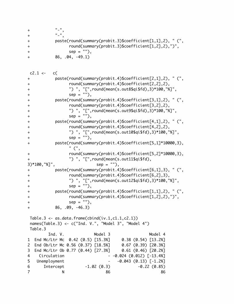
+ "-",+ "-",+ paste(round(summary(probit.3)$coefficient[1,1],2), " (",+ round(summary(probit.3)$coefficient[1,2],2),")",+ sep = ""),+ 86, .04, -49.1) c2.1 <- c(+ paste(round(summary(probit.4)$coefficient[2,1],2), " (", + round(summary(probit.4)$coefficient[2,2],2), + ") ", "[",round(mean(s.out8$qi$fd),3)*100,"%]", + sep = ""),+ paste(round(summary(probit.4)$coefficient[3,1],2), " (", + round(summary(probit.4)$coefficient[3,2],2), + ") ", "[",round(mean(s.out9$qi$fd),3)*100,"%]", + sep = ""),+ paste(round(summary(probit.4)$coefficient[4,1],2), " (", + round(summary(probit.4)$coefficient[4,2],2), + ") ", "[",round(mean(s.out10$qi$fd),3)*100,"%]", + sep = ""),+ paste(round(summary(probit.4)$coefficient[5,1]*10000,3), " (", + round(summary(probit.4)$coefficient[5,2]*10000,3), + ") ", "[",round(mean(s.out11$qi$fd),3)*100,"%]", sep = ""),+ paste(round(summary(probit.4)$coefficient[6,1],3), " (", + round(summary(probit.4)$coefficient[6,2],3), + ") ", "[",round(mean(s.out12$qi$fd),3)*100,"%]",+ sep = ""),+ paste(round(summary(probit.4)$coefficient[1,1],2), " (",+ round(summary(probit.4)$coefficient[1,2],2),")",+ sep = ""),+ 86, .09, -46.3) Table.3 <- as.data.frame(cbind(iv.1,c1.1,c2.1)) names(Table.3) <- c("Ind. V.", "Model 3", "Model 4") Table.3 Ind. V. Model 3 Model 41 End Mc/Ltr Mc 0.42 (0.5) [15.3%] 0.38 (0.54) [13.2%]2 End Ob/Ltr Mc 0.56 (0.37) [18.5%] 0.67 (0.39) [20.3%]3 End Mc/Ltr Ob 0.77 (0.44) [27.3%] 0.61 (0.46) [20.2%]4 Circulation - -0.024 (0.012) [-13.4%]5 Unemployment - -0.043 (0.13) [-1.2%]6 Intercept -1.02 (0.3) -0.22 (0.85)7 N 86 86

8 Pseudo R2 0.04 0.099 Log-Likelihood -49.1 -46.3 #Print Table 4 iv.2 <- c('Letter/Endorse Diff', 'Circulation(10000s)', 'Unemployment', 'Intercept', 'N', 'Pseudo R2', 'Log-Likelihood') c1.2 <- c(+ paste(round(summary(probit.5)$coefficient[2,1],2), " (", + round(summary(probit.5)$coefficient[2,2],2), + ") ", "[",round(mean(s.out13$qi$fd),3)*100,"%]", + sep = ""), "-", "-", + paste(round(summary(probit.5)$coefficient[1,1],2), " (",+ round(summary(probit.5)$coefficient[1,2],2),")",+ sep = ""), 86, .03, -49.6) c2.2 <- c(+ paste(round(summary(probit.6)$coefficient[2,1],2), " (", + round(summary(probit.6)$coefficient[2,2],2), + ") ", "[",round(mean(s.out14$qi$fd),3)*100,"%]", + sep = ""),+ paste(round(summary(probit.6)$coefficient[3,1]*10000,3), " (", + round(summary(probit.6)$coefficient[3,2]*10000,3), + ") ", "[",round(mean(s.out15$qi$fd),3)*100,"%]", + sep = ""), + paste(round(summary(probit.6)$coefficient[4,1],2), " (", + round(summary(probit.6)$coefficient[4,2],2), + ") ", "[",round(mean(s.out16$qi$fd),3)*100,"%]", + sep = ""), + paste(round(summary(probit.6)$coefficient[1,1],2), " (", + round(summary(probit.6)$coefficient[1,2],2), + ")", + sep = ""), 86, .08, -46.7) Table.4 <- as.data.frame(cbind(iv.2,c1.2,c2.2)) names(Table.4) <- c("Ind. V.", "Model 5", "Model 6") Table.4 Ind. V. Model 5 Model 61 Letter/Endorse Diff 0.49 (0.3) [15.3%] 0.53 (0.31) [15%]2 Circulation(10000s) - -0.023 (0.012) [-13.7%]3 Unemployment - -0.07 (0.13) [-1.9%]4 Intercept -0.88 (0.24) 0.02 (0.77)5 N 86 866 Pseudo R2 0.03 0.087 Log-Likelihood -49.6 -46.7

#open data butlerschofield apr 2010 liberal media...

Documents