open model files

Open Model Files Topics in this section

Introduction Open Autodesk Simulation Models Open CAD Files FEA Model Import and Export Functionality Archives Open Model Files from CDs After You Open a Model

Introduction You cannot open or save files with a filename, including the file path, that exceeds 200 characters. Windows limits paths to 260 bytes which is approximately 260 characters. Autodesk Simulation further limits the number of characters to allow for appended characters required for reports and other bookkeeping tasks. If you are unable to open a file, move the applicable files and folders to a different location.

Open Autodesk Simulation Models Autodesk Simulation uses .fem files to save FEA models (mesh, tree view information, and more).

The format of the .fem file changed at version 20. If you use the .fem file to open a model earlier than version 20, it is treated the same as opening a legacy model. See the following for more information.

Open models

1. Click Open.

2. Set the Files of type to Autodesk Simulation FEA Model (*.fem).

3. Browse to the appropriate file and click Open.

You can also drag a file into an open Autodesk Simulation window. NoteSet the Files of type to Autodesk Simulation Archive (*.ach) to retrieve an archive. Autodesk Simulation decompresses the archive and opens the model. For more information, see Archives.

Open legacy models

Files prior to version 20, store the Autodesk Simulation model in .dmit files (copy of CAD parts), .esx and .fem files (the mesh), and .esd files (Superdraw III mesh). Opening any of these file types converts the old model to the new format. We recommend that you back up your archive as the conversion is not reversible.

Files prior to release 12 store the Autodesk Simulation model in a file without an extension (the dot nothing file). You can import these models using the standalone program DotNothing2FEM.exe that we provide in the Autodesk Simulation installation folder. Open these old models as follows:

1. Double-click DotNothing2FEM.exe in the Autodesk Simulation installation folder.

2. In the Legacy Model Updater dialog box, click the button for the Legacy filename. Browse to your file and click Open.

3. The new model name displays in the FEM filename field. Keep the name or enter a new name.

4. Click Update to begin the conversion process. The status area indicates various stages in the conversion process.

5. During the conversion, review the converter log file, click Done, and select a unit system. (Prior to release 12, models did not use a unit system.)

6. The status area of the Legacy Model Updater dialog box is blank when the conversion is complete.

7. Use Autodesk Simulation to open the .fem file. ImportantThe conversion process does not read the following items from the original model. Inspect the model and enter the appropriate data

Element normal coordinate of plate-like elements (entered in the Element Definition). The coordinate controls things such as the direction of pressure loads, temperature gradient through the thickness, and stacking sequence of composite element laminae.

The gravity direction multipliers (entered in the Analysis Parameters). The old releases stored this data in a fashion that is not compatible with the current software.

Open CAD Files Work Locally

Save models on a local drive not a network location. If the CAD model is on a network drive, transfer the model to Autodesk Simulation, and then use the Save As command to save the FEA model to the local computer.

CAD models are solid models with surface information or wire frame models. The CAD solid models can be automatically meshed using the capabilities of the Autodesk Simulation user interface. Wire frame models cannot be meshed automatically (except for flat, 2D models) and are typically used for line elements or as edges of hand meshed models.

A CAD model cannot be opened from the user interface or transferred from the CAD package to the user interface if any of the following conditions are true:

If a legacy .DMIT file exists at the destination import location having the same file name.

If a legacy .ESX file exists at the destination import location having the same file name.

If a legacy .FEM file exists at the destination import location having the same file name.

If any of the above are true, the import will be aborted. In some cases, you are informed that they first need to convert their legacy model by opening it. After the old model is converted, the new CAD model can be imported.

When dealing with CAD solid models, follow these guidelines to avoid FEA modeling issues.

Guideline Notes

Use the proper element type.

CAD solid models are generally used to generate brick elements, but parts with thin walls do not always give the best results with brick elements. Thin-walled models may give more accurate results if used to generate plate elements. This may influence how much detail is put into the CAD solid model.

Remove parts that are not relevant to the stress calculations.

Simplify complicated assemblies by eliminating some parts. The only reason some parts are in an assembly is to prevent other parts from moving in a particular direction. Replace them by properly constraining the model. Other parts are simply there to connect two parts together, such as screws and pins. These types of connections can be simulated more efficiently by connecting the nodes of the parts together (replacing the screw) or by using other element types, like beam and truss elements (replacing the pin).

Remove unnecessary details.

Many assemblies have small features such as fillets or holes that will not affect the results. To accurately represent such features, they will require a finer mesh size in those areas, which could result in significantly more elements. Remove these features to reduce the analysis time. Most complex features can be suppressed in the CAD software by selecting the Simplify Model command. You can suppress features individually or globally in the model through the use of sliders.

Split surfaces Many loads in Autodesk Simulation are applied to surfaces of a model. If a load applies to only a portion of a large face, split the surface in the CAD software. It places the region to be loaded on a unique face which will remain a unique surface. (Check the documentation for your CAD software. See split lines, imprint, split face, split part, and project geometry.) Another use of splitting a surface would be to control how the surfaces are created along a cylindrical hole. Most CAD packages create two semicircular surfaces. and rotate them 90 degrees from how you would need them to properly apply a

load.

Topics in this section Import CAD Solid Models with CAD Application Import CAD Solid Models without CAD Application Surface Knitting Import CAD Wireframe Files

Import CAD Solid Models with CAD Application

To read CAD solid models from CAD packages, Autodesk Simulation uses Direct Memory Image Transfer (DMIT) technology. DMIT captures geometry information directly from memory while the CAD model is open in its respective program, and saves it to the Autodesk Simulation .fem file.

Supported CAD solid modelers are as follows. The latest version tested is listed. Older versions may work properly but are not guaranteed. (If an older version does not work, save the CAD model to a neutral file format -- such as .SAT, .STP or .STEP -- and open the neutral file with Autodesk Simulation.)

Alibre Design (version 12)

Autodesk Inventor (version 2011)

Autodesk Inventor Fusion (version 2011)

Autodesk Mechanical Desktop (version 2009)

CoCreate OneSpace Modeling (version 2008)

IronCAD (V11 Product Update 1)

KeyCreator (version 8.5)

Pro/ENGINEER (Wildfire 4.0)

Rhinoceros® (version 4)

Solid Edge (V20)

Solid Edge with Synchronous Technology (V100)

SolidWorks (version 2009)

SpaceClaim (version 2009)

When importing the file into Autodesk Simulation, you may be prompted with the Surface Knitting dialog. See the page Surface Knitting for details.

In normal cases, the CAD model will be sent to first session of Autodesk Simulation, replacing any model currently in the software. However, if the first session of Autodesk Simulation is meshing or analyzing the model, a new session with be opened, and the CAD model will be transferred to the new session.

Import files using Autodesk Simulation with CAD package installed

Use one of the following procedures:

1. Click Open.

2. Set the Files of type to the appropriate setting (SolidWorks part, Pro/ENGINEER part, and so on).

3. Click Options to set any available options to use when opening the file.

4. The CAD program opens the selected file in silent mode and transfers the parts to Autodesk Simulation.

After the file imports correctly, the Model Mesh Settings dialog box displays. NoteWhen opening an older KeyCreator file with a newer version of KeyCreator, an upgrade notice stalls the transfer process. Respond to the upgrade notice to continue silent transfer process.

OR

You can drag and drop the CAD file into an open Autodesk Simulation window.

Import files using Alibre Design

1. After installing the software, there is an Autodesk Simulation option in the Tools: Addons menu.

2. Select Autodesk Simulation to transport the model into the FEA Editor environment.

For Alibre V11 and on, assembly-level features are transferred to Autodesk Simulation. For example, drilling a hole through 2 parts in the assembly are included in the transfer; the hole does not need to be put into each part separately.

Import files using Autodesk Inventor

1. After installing the software, there is an Autodesk Simulation panel in the Inventor Tools tab.

2. Select Start Simulation to transport the model into the FEA Editor environment.

Work points defined in Inventor are transferred to Autodesk Simulation as construction vertices. The mesh will place nodes at the construction vertices. (See Construction Vertices -Seed Points.) Note that Inventor always has a work point at the origin, so this will create a construction vertex at the origin in Autodesk Simulation.

The following material properties defined in Inventor are transferred to Autodesk Simulation and assigned to the parts. Note that additional material properties may need to be entered in Autodesk Simulation to perform that analysis.

Mass density

Modulus of elasticity

Poisson's ratio

Thermal expansion coefficient

Yield strength

Ultimate tensile strength

Thermal conductivity

Specific Heat

Import files using Autodesk Inventor Fusion

After installing the software, there is a Simulation panel on the Home tab of the ribbon. Select Autodesk Simulation to transport the model into the FEA Editor environment.

Material properties defined in Fusion are transferred to Autodesk Simulation and assigned to the parts. Note that additional material properties may need to be entered in Autodesk Simulation.

For more information about Inventor Fusion, visit https://labs.autodesk.com/technologies/fusion/.

Import files using Autodesk Mechanical Desktop

1. After installing the software, there is an Autodesk Simulation menu in the Mechanical Desktop menus.

2. Select Simplify Model in the Autodesk Simulation menu to suppress some of the complex features in the model (fillets, dimensions, and so on). Alternatively, type AlgorFeatureControl in the command line.

3. Select Start Simulation from Autodesk Simulation menu to transport the model into the FEA Editor environment. Alternatively, type AlgorMesh in the command line.

NoteIf the Autodesk Simulation menu does not appear, see CAD Setup and Troubleshooting for instructions.

Import files using CoCreate OneSpace Modeling

1. After installing the software, there will be an Autodesk Simulation Mesh option in the Tools: Toolbox Application menu.

2. Select the part or parts to be transferred to Autodesk Simulation. (Highlight parts in Structure Browser, right-click and choose Apply Selection.)

3. Select the Autodesk Simulation Mesh sub menu in the Tools: Toolbox Application menu.

4. Select the confirmation checkmark from the task panel slide out.

5. A standard Windows Save dialog will appear. Choose a location and filename for the analysis.

6. The model is exported to Autodesk Simulation when the Save button is clicked. NoteIf the Autodesk Simulation menu does not appear, see CAD Setup and Troubleshooting for instructions.

Import files using IronCAD

1. After installing the software, there will be an Autodesk Simulation pull-down menu.

2. Select the Start Simulation command to transport the model into the FEA Editor environment.

Assembly-level features are transferred to Autodesk Simulation. For example, drilling a hole through 2 parts in the assembly will be included in the transfer; the hole does not need to be put into each part separately.

Import files using KeyCreator

1. After installing the software, there will be an Autodesk Simulation FEA add-in pull-out menu in the ADD-INS pull-down menu.

2. Select the Autodesk Simulation pull-out menu and select the Start Simulation command.

3. Select the parts to transfer by following the prompts in KeyCreator.

4. Click the Accept button to transport the model into the FEA Editor environment. NoteIf the Autodesk Simulation menu does not appear, see CAD Setup and Troubleshooting for instructions.

Import files using Pro/ENGINEER

1. After installing the software, there will be an Autodesk Simulation pull-down menu in the Pro/ENGINEER pull-down menus.

2. Select the Simplify Model command in the Autodesk Simulation pull-down menu to suppress some of the complex features in the model (fillets, dimensions, and so on) if appropriate.

3. Select the Start Simulation command in the Autodesk Simulation pull-down menu to transport the model into the FEA Editor environment.

Datum points defined in Pro/ENGINEER are transferred to Autodesk Simulation as construction vertices. The mesh will place nodes at the construction vertices. (See Construction Vertices -Seed Points in the section Meshing Overview: Meshing CAD Solid Models.)

NoteIf the Autodesk Simulation menu does not appear, see CAD Setup and Troubleshooting for instructions.

Import files using Rhinoceros

1. After installing the software, there will be an Autodesk Simulation pull-down menu in the Rhinoceros pull-down menus.


Import files using Solid Edge

1. After installing the software, there will be an Autodesk Simulation pull-down menu in the Solid Edge pull-down menus.



Part, Assembly, Sheet Metal, or Weldment models can be meshed in Autodesk Simulation.

The Autodesk Simulation pull-down menu in Solid Edge contains an Automatic update option. If this is active, anytime you make a geometry change to the model in Solid Edge, it will be automatically sent to Autodesk Simulation and any meshing functions that were previously performed will be performed again. If this option is not active, you will need to use the Autodesk Simulation: Start Simulation command again to update the Autodesk Simulation model. NoteLegacy Solid Edge assemblies may need to be reconstructed in the current version in order for the mates to be correct. If parts are not positioned properly when imported into Autodesk Simulation, redo the assembly mates in Solid Edge. ImportantSolid Edge pays attention to the activation and visibility status of the assembly components. Only parts that are active and visible are transferred to Autodesk Simulation.

Import files using SolidWorks

1. After installing the software, there will be an Autodesk Simulation pull-down menu in the SolidWorks pull-down menus.



Any material properties defined in SolidWorks will be transferred to Autodesk Simulation and assigned to the parts. Note that additional material properties may need to be entered in Autodesk Simulation to perform that analysis.

Assembly-level features are transferred to Autodesk Simulation. For example, drilling a hole through 2 parts in the assembly will be included in the transfer; the hole does not need to be put into each part separately.

Import files using SpaceClaim

1. After installing the software, there will be an Autodesk Simulation Mesh tab in the SpaceClaim ribbon bar.

2. Select the Autodesk Simulation: Start Simulation command to transport the model into the FEA Editor environment. Note that visible and invisible parts are transferred.

The following material properties defined in SpaceClaim will be transferred to Autodesk Simulation and assigned to the parts. Note that additional material properties may need to be entered in Autodesk Simulation to perform that analysis.

Mass density

Modulus of elasticity

Poisson's ratio

Thermal expansion coefficient

Ultimate tensile strength

Thermal conductivity

Specific Heat NoteModels that contain the following characters, either in the name of the file or in any folder through the path to where the file is stored, may not transfer to Autodesk Simulation: = ( )

Associativity between CAD and Autodesk Simulation

Once you have meshed a CAD model, a connection will be created and maintained between the CAD model and the Autodesk Simulation model. If the CAD package and Autodesk Simulation remain opened and if the CAD model is revised, the Autodesk Simulation model will be automatically surface meshed with the previous meshing settings after the CAD model is transferred. (The previous mesh settings that are retained include the mesh size, refinement points, construction vertices, and so on.) If the CAD package or Autodesk Simulation is closed, then you will need to initiate the meshing process after the CAD model is transferred. (The same mesh settings are retained though.) The CAD packages which support associativity are as follows:

CAD Package Surface Associativity Edge Associativity

Alibre Yes Yes

Autodesk Inventor Yes Yes

Autodesk Inventor Fusion Yes Yes

Autodesk Mechanical Desktop No No

CoCreate OneSpace Modeling Yes No

IronCAD Yes No

KeyCreator (7.0.2 and later) Yes No

Pro/ENGINEER Yes No

Rhinoceros Yes No

Solid Edge Yes No

SolidWorks Yes No

SpaceClaim Yes No

For CAD applications that transfer material properties to Autodesk Simulation, use the Tools: Options: CAD Import tab, Global CAD Import Options to control whether the

CAD materials remain associative with Autodesk Simulation when the CAD model is changed or not. For more information, see CAD Import Tab. NoteThe units of the CAD model are also transferred to Autodesk Simulation. In many cases, only the units of length are set in the CAD, so the other units (energy, time, temperature, and so on) are set in Autodesk Simulation. You can change these as needed by right-clicking on the Model Units entry in the tree view and choosing Edit: Current Modeling Units. If the units of length are changed in Autodesk Simulation and the CAD model is transferred again, the length units will be set back to the units in the CAD model. Thus, the length units are associative. (This is required since the original units are the dimensions of the model.) If any other unit is changed in Autodesk Simulation, it will not be changed if the CAD model is transferred again. Other units are not associative. NoteWhen opening an older KeyCreator file with a newer version of KeyCreator, an upgrade notice will be presented to save the file to the current version. If you answer No to not upgrade the file, then this file will not have associativity with Autodesk Simulation. Answering Yes will allow associativity.

The CAD packages that support surface associativity will maintain surface based loads and surface based boundary conditions when a revised model is transferred to Autodesk Simulation. Packages that do not support surface associativity will need to have surface loads re-applied after a revised model is transferred. (The surface loads will be maintained in all cases if the model is simply remeshed.)

The CAD packages that support edge associativity will maintain edge loads and edge boundary conditions when a revised model is transferred to Autodesk Simulation. Packages that do not support edge associativity will need to have edge loads re-applied when a revised model is transferred. (The edge loads will be maintained in all cases if the model is simply remeshed.)

Nodal loads and boundary conditions are not associative with the CAD model and will need to be reapplied if a revised model is transferred to Autodesk Simulation. (The nodal loads will also need to be re-applied if the model is simply remeshed.)

Topics in this section Simplify Model

Simplify Model

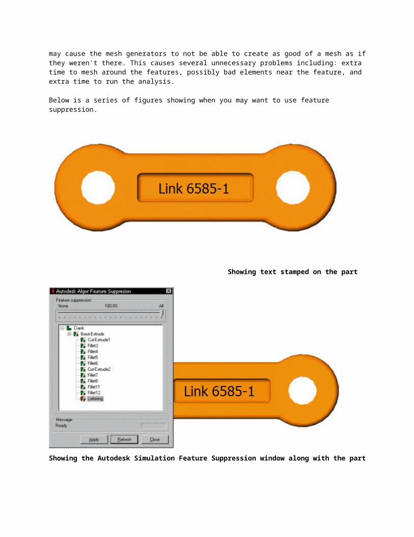
In the Autodesk Simulation menu for some of the CAD systems for which a direct transfer exists, there is a command entitled Simplify Model. This command will allow you to suppress any feature in your CAD model that is not necessary for the FEA model.

Use feature suppression to remove small details from your model that will not affect the results of an analysis. These small details if left in the model may cause the mesh generators to not be able to create as good of a mesh as if they weren't there. This causes several unnecessary problems including: extra time to mesh around the features, possibly bad elements near the feature, and extra time to run the analysis.

Below is a series of figures showing when you may want to use feature suppression.

Showing text stamped on the part

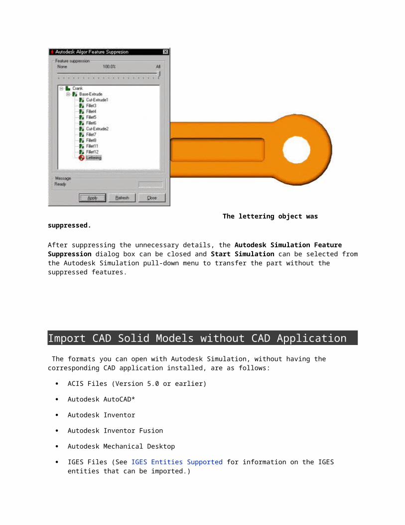
Showing the Autodesk Simulation Feature Suppression window along with the part

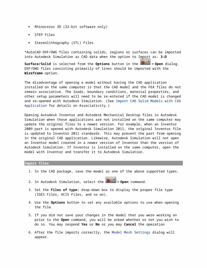
The lettering object was suppressed.

After suppressing the unnecessary details, the Autodesk Simulation Feature Suppression dialog box can be closed and Start Simulation can be selected from the Autodesk Simulation pull-down menu to transfer the part without the suppressed features.

Import CAD Solid Models without CAD Application The formats you can open with Autodesk Simulation, without having the corresponding CAD application installed, are as follows:

ACIS Files (Version 5.0 or earlier)

Autodesk AutoCAD*

Autodesk Inventor

Autodesk Inventor Fusion

Autodesk Mechanical Desktop

IGES Files (See IGES Entities Supported for information on the IGES entities that can be imported.)

Rhinoceros 3D (32-bit software only)

STEP Files

Stereolithography (STL) Files

*AutoCAD DXF/DWG files containing solids, regions or surfaces can be imported into Autodesk Simulation as CAD data when the option to Import as: 3-D Surface/Solid is selected from the Options button in the Open dialog. DXF/DWG files consisting primarily of lines should be imported with the Wireframe option.

The disadvantage of opening a model without having the CAD application installed on the same computer is that the CAD model and the FEA files do not remain associative. The loads, boundary conditions, material properties, and other setup parameters will need to be re-entered if the CAD model is changed and re-opened with Autodesk Simulation. (See Import CAD Solid Models with CAD Application for details on Associativity.)

Opening Autodesk Inventor and Autodesk Mechanical Desktop files in Autodesk Simulation when those applications are not installed on the same computer may update the original files to a newer version. For example, when an Inventor 2009 part is opened with Autodesk Simulation 2011, the original Inventor file is updated to Inventor 2011 standards. This may prevent the part from opening in the original CAD application. Likewise, Autodesk Simulation will not open an Inventor model created in a newer version of Inventor than the version of Autodesk Simulation. If Inventor is installed on the same computer, open the model with Inventor and transfer it to Autodesk Simulation.

Import files

1. In the CAD package, save the model as one of the above supported types.

2. In Autodesk Simulation, select the Open command.

3. Set the Files of type: drop-down box to display the proper file type (IGES Files, ACIS Files, and so on).

4. Use the Options button to set any available options to use when opening the file.

5. If you did not save your changes in the model that you were working on prior to the Open command, you will be asked whether or not you wish to do so. You may respond Yes or No or you may Cancel the operation

6. After the file imports correctly, the Model Mesh Settings dialog will appear.

Drag-and-drop technology is also supported, so you can simply drag the file onto the Autodesk Simulation icon on the Windows Desktop, or into an open Autodesk Simulation window, and the software will take care of the rest.

When importing the file, you may be prompted with the Surface Knitting dialog. See the page Surface Knitting for details. NoteSee Application Menu: Options Dialog Box: CAD Import Tab for details on the available options.

STEP files

STEP files might be saved in a different unit of length than shown by the CAD software. (This functionality varies from CAD package to package.) Use the Open Options command to control whether the STEP file is converted to a different unit of length when the

file is opened with Autodesk Simulation. (The Open Options command also includes an option about whether to prompt you for the units each time a STEP file is opened.) For example, the CAD model may be saved in units of centimeters from the CAD software even though the units in use were inches. If the model is not converted when opened with Autodesk Simulation, the units of length will be centimeters, and this would require all input that uses a length unit to use centimeters, such as moments (force*cm), modulus of elasticity (force/cm2), thermal conductivity (energy/(cm*time*degree)), and so on.

Scaling the STEP file from the original units to a new unit also scales any inaccuracies in the file. If the model is scaled by a large amount, such as from centimeters to microns (a factor of 1E4) or from meters to microns (a factor of 1E6), then problems may occur with feature matching and other tolerances which could prevent the model from meshing.

Topics in this section IGES Entities Supported

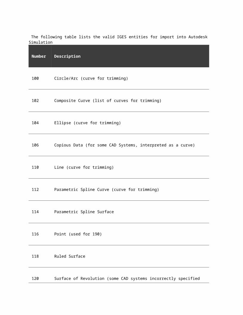
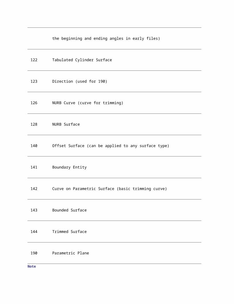
IGES Entities Supported The following table lists the valid IGES entities for import into Autodesk Simulation

Number Description

100 Circle/Arc (curve for trimming)

102 Composite Curve (list of curves for trimming)

104 Ellipse (curve for trimming)

106 Copious Data (for some CAD Systems, interpreted as a curve)

110 Line (curve for trimming)

112 Parametric Spline Curve (curve for trimming)

114 Parametric Spline Surface

116 Point (used for 190)

118 Ruled Surface

120Surface of Revolution (some CAD systems incorrectly specified the beginning and ending angles in early files)

122 Tabulated Cylinder Surface

123 Direction (used for 190)

126 NURB Curve (curve for trimming)

128 NURB Surface

140 Offset Surface (can be applied to any surface type)

141 Boundary Entity

142 Curve on Parametric Surface (basic trimming curve)

143 Bounded Surface

144 Trimmed Surface

190 Parametric Plane

Note

Autodesk Simulation only uses 141/143 and 142/144 combinations to describe trimmed surfaces.

The IGES file also supports some representation of B-Rep solids (186) that are not supported by Autodesk Simulation

Surface Knitting When a CAD solid model is imported or opened, the Surface Knitting dialog can appear. Surface knitting is a process of recognizing where two parts have surfaces in contact, and then splitting the surfaces if necessary to get identical surfaces. The benefits of choosing to knit the surfaces are as follows:

The matching of the meshes on adjacent surfaces is better if the surfaces are identical. However,

The Mesh Mesh 3D Mesh Settings Options Model Use virtual imprinting will create a quality matched mesh without using surface knitting. See the page Meshing Overview: Meshing CAD Solid Models: Model Mesh Settings: Model for details.

For analysis types that support smart bonding, it is not strictly necessary to have a matched mesh. See the page Meshing Overview: Creating Contact Pairs: Types of Contact for the analysis types that support smart bonding.

Some loads should only be applied to free or exposed surfaces, such as pressure and convection. If a large surface is not split where it is covered by other parts, then the load will be applied to a larger area than intended. See the figures below.

Surface knitting must be used if the Fluid Generation is going to be used (create a new part from the solid parts to use in a fluid analysis).

TipThe Surface Knitting dialog is not activated by default. If it is not activated, the dialog will not be displayed when a CAD model is imported or opened. To display the Surface Knitting dialog, use Options CAD Import Global CAD Import Options and set the Knit surfaces on import: option to Yes before opening the CAD model.

When merging a CAD model into a CAD model, do not choose to knit the merged model if the original model was not knitted. NoteSurface knitting is not available for Rhino files.

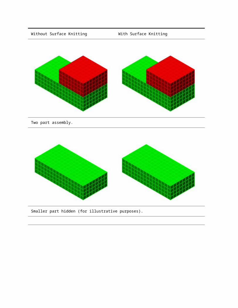
Without Surface Knitting With Surface Knitting

Two part assembly.

Smaller part hidden (for illustrative purposes).

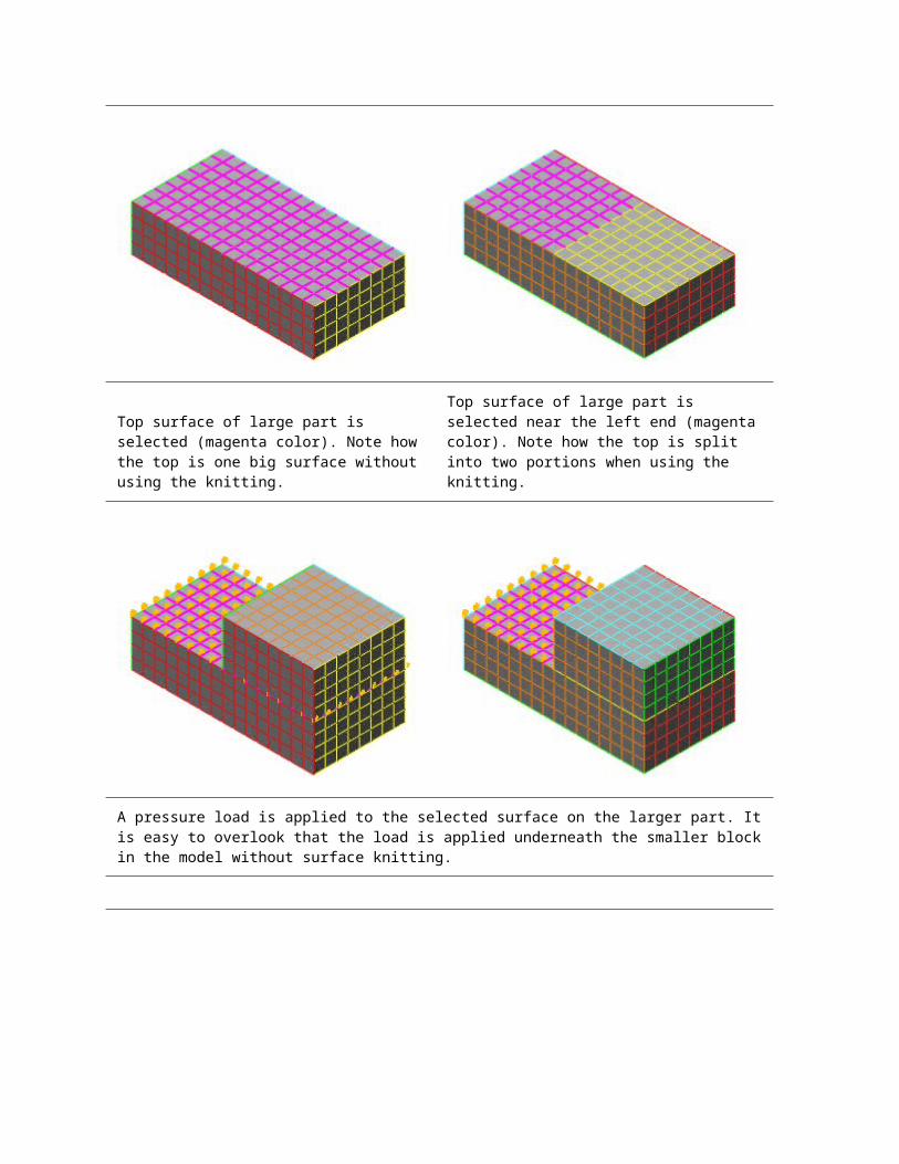
Top surface of large part is selected (magenta color). Note how the top is one big surface without using the knitting.

Top surface of large part is selected near the left end (magenta color). Note how the top is split into two portions when using the knitting.

A pressure load is applied to the selected surface on the larger part. It is easy to overlook that the load is applied underneath the smaller block in the model without surface knitting.

In the Results environment (with Transparency used on the smaller part), it can be seen that the pressure is applied over the entire face.

In the Results environment (with Transparency used on the smaller part), it can be seen that the pressure is applied over the intended region. The pressure is not applied under the smaller part.

Although some CAD programs have the ability to split a face or surface into smaller regions, surface knitting provides an alternative method of creating a split face. (For those CAD packages that do not provide the ability to split a face, surface knitting in Autodesk Simulation is the only practical method.) Imagine that the part being modeled is welded to a round support piece, and the support piece is not needed in the analysis. However, the pattern of the round support is needed in the mesh of the model to apply the boundary conditions. Using the surface knitting feature, the method of creating this would be as follows:

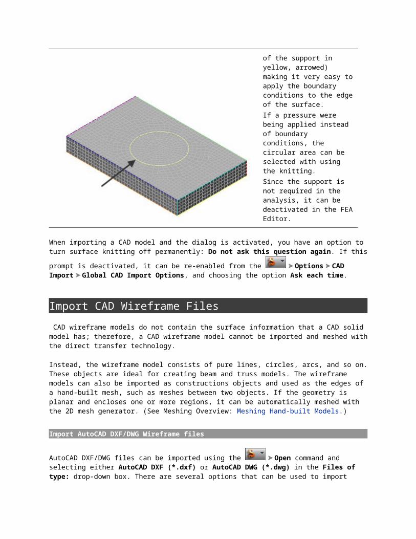
A wire frame view of one of the parts in a hypothetical analysis. Boundary conditions are desired on the part around the circular feature (arrowed) on the face. (This is simulating the weld between this part and the support which is not included in the analysis.) Without putting some kind of feature in the CAD solid model, such as splitting the face or adding a fictitious step, the part would import and mesh without having the nodes in the circular pattern. The mesh would be a rectangular pattern on all 6 faces of the solid, and there would only be 6 surfaces on the part.

By adding the support to the CAD solid model and importing into Autodesk Simulation, the circular pattern desired for the boundary conditions is created by the mesh matching.

Furthermore, by using the surface knitting during the import, the rectangular face is split into a surface of a rectangle with a hole and a surface of a circle.

This also adds new edges to the model (the perimeter of the support in yellow, arrowed) making it very easy to apply the boundary conditions to the edge of the surface. If a pressure were being applied instead of boundary conditions, the circular area can be selected with using the knitting. Since the support is not required in the analysis, it can be deactivated in the FEA Editor.

When importing a CAD model and the dialog is activated, you have an option to turn surface knitting off permanently: Do not ask this question again. If this prompt is deactivated, it can be re-enabled from the Options CAD Import Global CAD Import Options, and choosing the option Ask each time.

Import CAD Wireframe Files CAD wireframe models do not contain the surface information that a CAD solid model has; therefore, a CAD wireframe model cannot be imported and meshed with the direct transfer technology.

Instead, the wireframe model consists of pure lines, circles, arcs, and so on. These objects are ideal for creating beam and truss models. The wireframe models can also be imported as constructions objects and used as the edges of a hand-built mesh, such as meshes between two objects. If the geometry is planar and encloses one or more regions, it can be automatically meshed with the 2D mesh generator. (See Meshing Overview: Meshing Hand-built Models.)

Import AutoCAD DXF/DWG Wireframe files

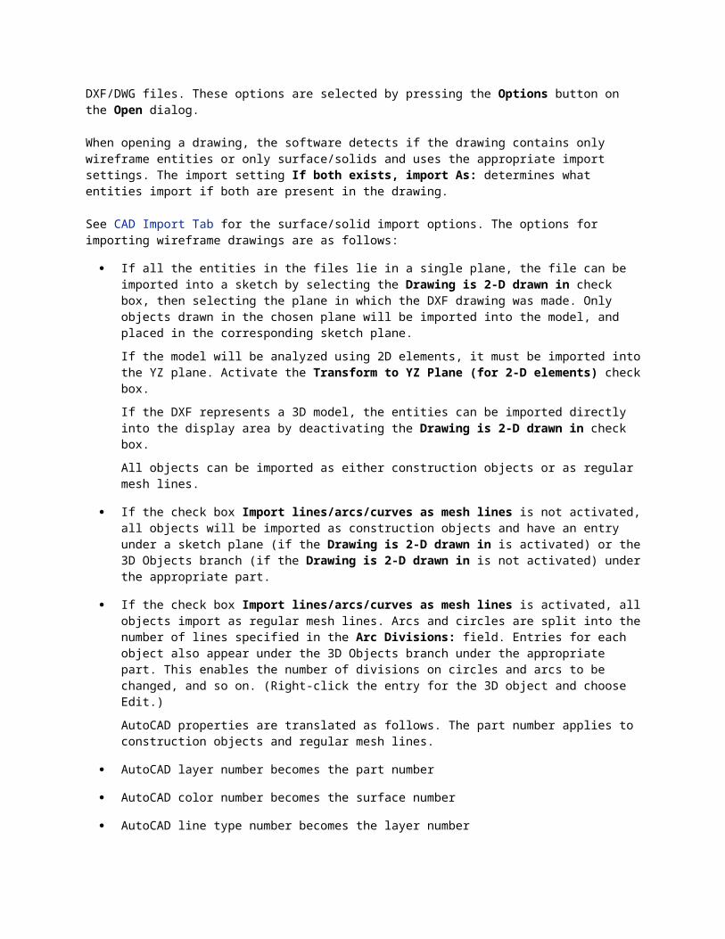
AutoCAD DXF/DWG files can be imported using the Open command and selecting either AutoCAD DXF (*.dxf) or AutoCAD DWG (*.dwg) in the Files of type: drop-down box. There are several options that can be used to import DXF/DWG files. These options are selected by pressing the Options button on the Open dialog.

When opening a drawing, the software detects if the drawing contains only wireframe entities or only surface/solids and uses the appropriate import settings. The import setting If both exists, import As: determines what entities import if both are present in the drawing.

See CAD Import Tab for the surface/solid import options. The options for importing wireframe drawings are as follows:

If all the entities in the files lie in a single plane, the file can be imported into a sketch by selecting the Drawing is 2-D drawn in check box, then selecting the plane in which the DXF drawing was made. Only objects drawn in the chosen plane will be imported into the model, and placed in the corresponding sketch plane. If the model will be analyzed using 2D elements, it must be imported into the YZ plane. Activate the Transform to YZ Plane (for 2-D elements) check box. If the DXF represents a 3D model, the entities can be imported directly into the display area by deactivating the Drawing is 2-D drawn in check box. All objects can be imported as either construction objects or as regular mesh lines.

If the check box Import lines/arcs/curves as mesh lines is not activated, all objects will be imported as construction objects and have an entry under a sketch plane (if the Drawing is 2-D drawn in is activated) or the 3D Objects branch (if the Drawing is 2-D drawn in is not activated) under the appropriate part.

If the check box Import lines/arcs/curves as mesh lines is activated, all objects import as regular mesh lines. Arcs and circles are split into the number of lines specified in the Arc Divisions: field. Entries for each object also appear under the 3D Objects branch under the appropriate part. This enables the number of divisions on circles and arcs to be changed, and so on. (Right-click the entry for the 3D object and choose Edit.) AutoCAD properties are translated as follows. The part number applies to construction objects and regular mesh lines.

AutoCAD layer number becomes the part number

AutoCAD color number becomes the surface number

AutoCAD line type number becomes the layer number

If the ID of an entity in the DXF file cannot be used in Autodesk Simulation, the entity will be placed with the number specified in the Replace Invalid _ IDs with: field. One common example of this is Layer 0 in AutoCAD. Entities cannot be placed in Part 0 in Autodesk Simulation.

If some entities are not connected properly in the sketch or 3D model, you can loosen the tolerance value. This can be done by activating the Use Tolerance check box and specifying a value in the adjacent field. All values beyond the decimal point specified will be truncated. For example, using the default tolerance of 1E-4, all digits at five decimal points or more will be truncated. The tolerance should only be used if initial import does not succeed.

DXF Entities Supported: 2D Sketches* 3D Models*

ARC ARC

CIRCLE CIRCLE

LINE LINE

POINT POLYLINE

SPLINE LWPOLYLINE

POLYLINE

LWPOLYLINE

*Files with entities not listed will still be imported. The non-supported entities will be ignored.

If your DXF/DWG file contains blocks, you have the option to Import Blocks As Separate Parts.

Import wireframe IGES files

Wireframe IGES files can be imported using the Open command and selecting the Wireframe IGES (*.igs, *.iges) option in the Files of type: drop-down box. There are different methods that can be used to wireframe files. These methods can be set by pressing the Options button on the Open dialog.

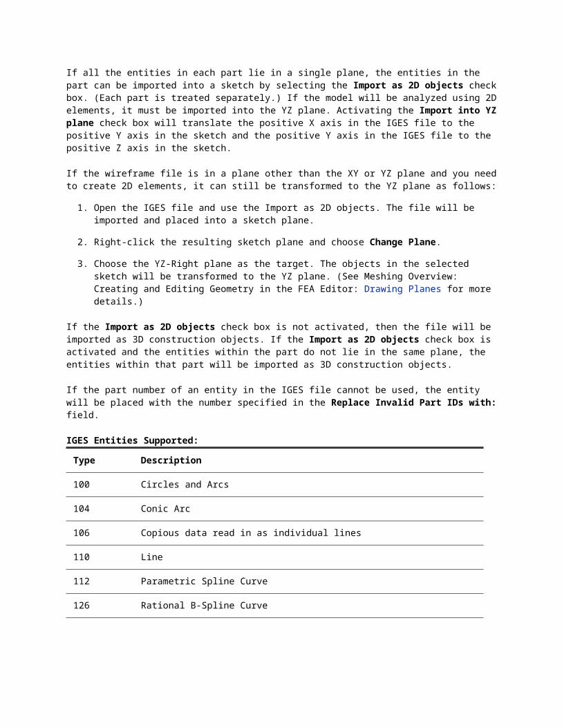
If all the entities in each part lie in a single plane, the entities in the part can be imported into a sketch by selecting the Import as 2D objects check box. (Each part is treated separately.) If the model will be analyzed using 2D elements, it must be imported into the YZ plane. Activating the Import into YZ plane check box will translate the positive X axis in the IGES file to the positive Y axis in the sketch and the positive Y axis in the IGES file to the positive Z axis in the sketch.

If the wireframe file is in a plane other than the XY or YZ plane and you need to create 2D elements, it can still be transformed to the YZ plane as follows:

1. Open the IGES file and use the Import as 2D objects. The file will be imported and placed into a sketch plane.

2. Right-click the resulting sketch plane and choose Change Plane.

3. Choose the YZ-Right plane as the target. The objects in the selected sketch will be transformed to the YZ plane. (See Meshing Overview: Creating and Editing Geometry in the FEA Editor: Drawing Planes for more details.)

If the Import as 2D objects check box is not activated, then the file will be imported as 3D construction objects. If the Import as 2D objects check box is activated and the entities within the part do not lie in the same plane, the entities within that part will be imported as 3D construction objects.

If the part number of an entity in the IGES file cannot be used, the entity will be placed with the number specified in the Replace Invalid Part IDs with: field.

IGES Entities Supported:

Type Description

100 Circles and Arcs

104 Conic Arc

106 Copious data read in as individual lines

110 Line

112 Parametric Spline Curve

126 Rational B-Spline Curve

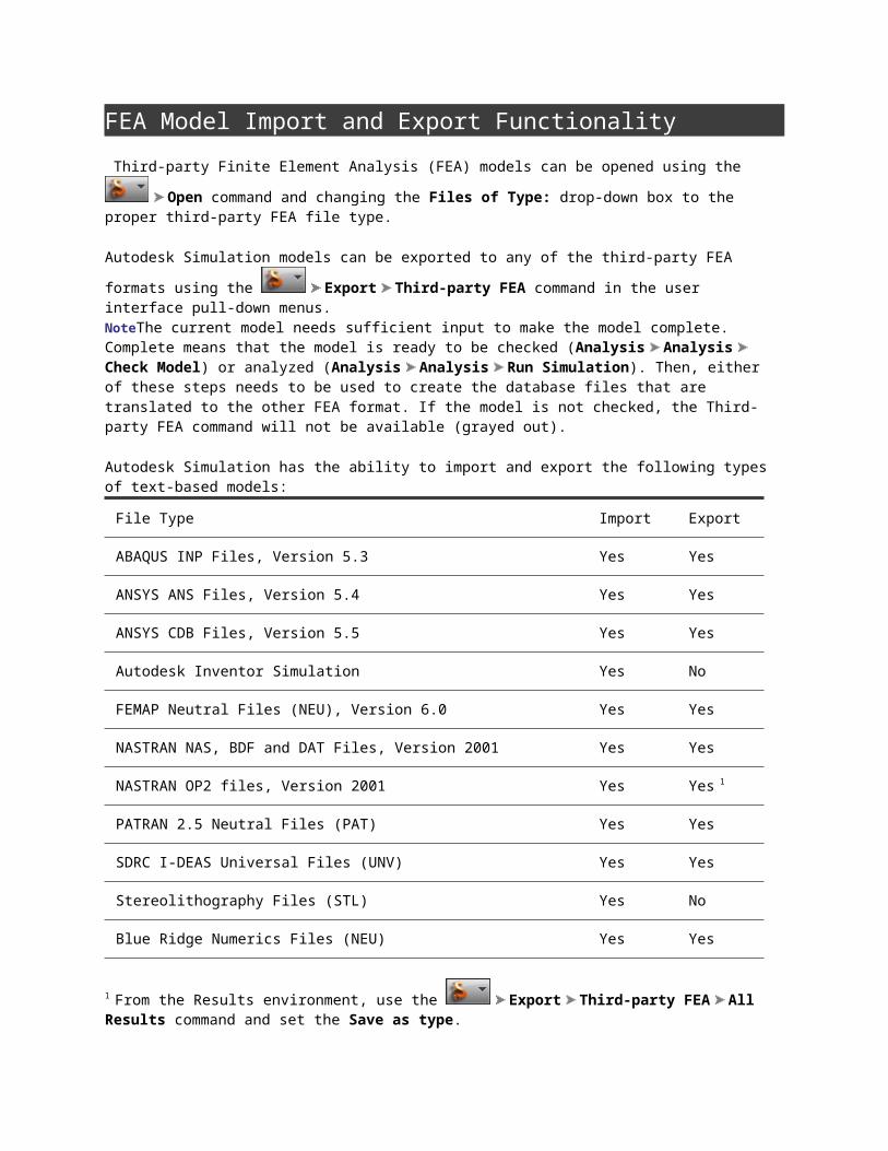
FEA Model Import and Export Functionality Third-party Finite Element Analysis (FEA) models can be opened using the Open command and changing the Files of Type: drop-down box to the proper third-party FEA file type.

Autodesk Simulation models can be exported to any of the third-party FEA formats using the Export Third-party FEA command in the user interface pull-down menus.

NoteThe current model needs sufficient input to make the model complete. Complete means that the model is ready to be checked (Analysis Analysis Check Model) or analyzed (Analysis Analysis Run Simulation). Then, either of these steps needs to be used to create the database files that are translated to the other FEA format. If the model is not checked, the Third-party FEA command will not be available (grayed out).

Autodesk Simulation has the ability to import and export the following types of text-based models:

File Type Import Export

ABAQUS INP Files, Version 5.3 Yes Yes

ANSYS ANS Files, Version 5.4 Yes Yes

ANSYS CDB Files, Version 5.5 Yes Yes

Autodesk Inventor Simulation Yes No

FEMAP Neutral Files (NEU), Version 6.0 Yes Yes

NASTRAN NAS, BDF and DAT Files, Version 2001 Yes Yes

NASTRAN OP2 files, Version 2001 Yes Yes 1

PATRAN 2.5 Neutral Files (PAT) Yes Yes

SDRC I-DEAS Universal Files (UNV) Yes Yes

Stereolithography Files (STL) Yes No

Blue Ridge Numerics Files (NEU) Yes Yes

1 From the Results environment, use the Export Third-party FEA All Results command and set the Save as type.

Topics in this section Abaqus ANSYS ANS Files ANSYS CDB Files Autodesk Inventor Simulation Blue Ridge Numerics FEMAP NASTRAN PATRAN SDRC Stereolithography

Abaqus Commands supported:

1. *NODE

2. *NSET

3. *NGEN

4. *NCOPY

5. *NFILL

6. *ELEMENT

7. *ELSET

8. *ELGEN

9. *ELCOPY

10. *MATERIAL

11. *SOLID

12. *SHELL

13. *ELASTIC

14. *DENSITY

15. *EXPANSION

16. *BOUNDARY

17. *CLOAD

18. *DLOAD

Some advanced node- and element-generation features have not been implemented.

The exact element types which are supported are:

1. Tetrahedra:

C3D10

C3D10H

C3D10R

C3D10I

C3D10T

C3D4

C3D4H

C3D4R

C3D4I

C3D4T

2. Bricks:

C3D20

C3D20H

C3D20R

C3D20I

C3D20T

C3D8

C3D8H

C3D8R

C3D8I

C3D8T

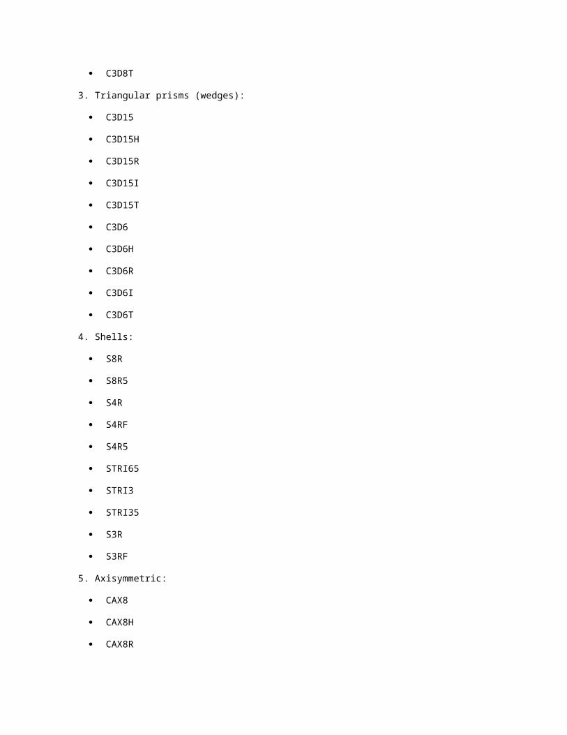
3. Triangular prisms (wedges):

C3D15

C3D15H

C3D15R

C3D15I

C3D15T

C3D6

C3D6H

C3D6R

C3D6I

C3D6T

4. Shells:

S8R

S8R5

S4R

S4RF

S4R5

STRI65

STRI3

STRI35

S3R

S3RF

5. Axisymmetric:

CAX8

CAX8H

CAX8R

CAX8RH

CAX4

CAX4H

CAX4R

CAX4RH

CAX6

CAX6H

CAX3

CAX3H

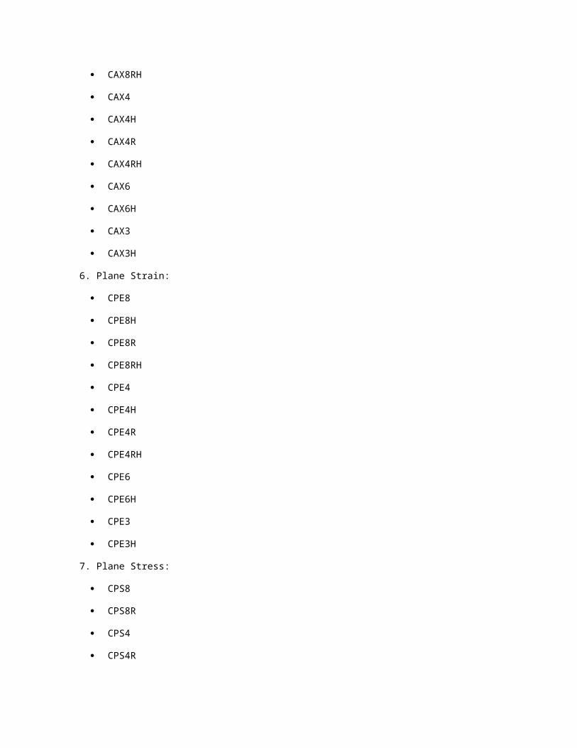
6. Plane Strain:

CPE8

CPE8H

CPE8R

CPE8RH

CPE4

CPE4H

CPE4R

CPE4RH

CPE6

CPE6H

CPE3

CPE3H

7. Plane Stress:

CPS8

CPS8R

CPS4

CPS4R

CPS6

CPS3

ANSYS ANS Files Commands supported:

1. /TITLE [export only]

2. N (node)

3. EN (element)

4. E (element, with no id)

5. EMORE (element continuation)

6. NBLOCK (node block)

7. EBLOCK (element block)

8. ET (element type definition)

9. TYPE (element type selector)

10. MP (material property)

11. R (element property value)

12. REAL (element property selector)

13. F (nodal load)

14. SFE (surface load)

15. D (boundary condition)


1. Handled as trusses:

LINK1

LINK8

PIPE16

PIPE20

LINK31

LINK32

LINK33

LINK34

PIPE59

LINK68

2. Handled as beams:

BEAM3

BEAM4

BEAM44

3. Handled as nonlinear beams:

BEAM23

BEAM24

BEAM54

4. Handled as membranes:

SHELL41

5. Handled as plates:

SHELL28

SHELL63

6. Handled as nonlinear shells:

SHELL43

SHELL57

SHELL93

7. Handled as sandwich (thick composites):

SOLID46

8. Handled as thin composites:

SHELL91

SOLID99

9. Handled as basic bricks:

SOLID5

SOLID45

HYPER58

SOLID64

SOLID65

SOLID73

HYPER86

VISCO107

10. Handled as enhanced bricks:

SOLID95

11. Handled as heat transfer bricks:

SOLID69

SOLID70

SOLID90

12. Handled as electrostatic bricks:

SOLID122

13. Handled as electrostatic tetrahedra:

SOLID123

14. Handled as electrostatic 2D

PLANE121

15. Handled as tetrahedra:

SOLID72

SOLID92

SOLID98

16. Handled as heat transfer tetrahedra:

SOLID87

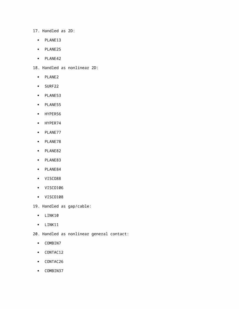
17. Handled as 2D:

PLANE13

PLANE25

PLANE42

18. Handled as nonlinear 2D:

PLANE2

SURF22

PLANE53

PLANE55

HYPER56

HYPER74

PLANE77

PLANE78

PLANE82

PLANE83

PLANE84

VISCO88

VISCO106

VISCO108

19. Handled as gap/cable:

LINK10

LINK11

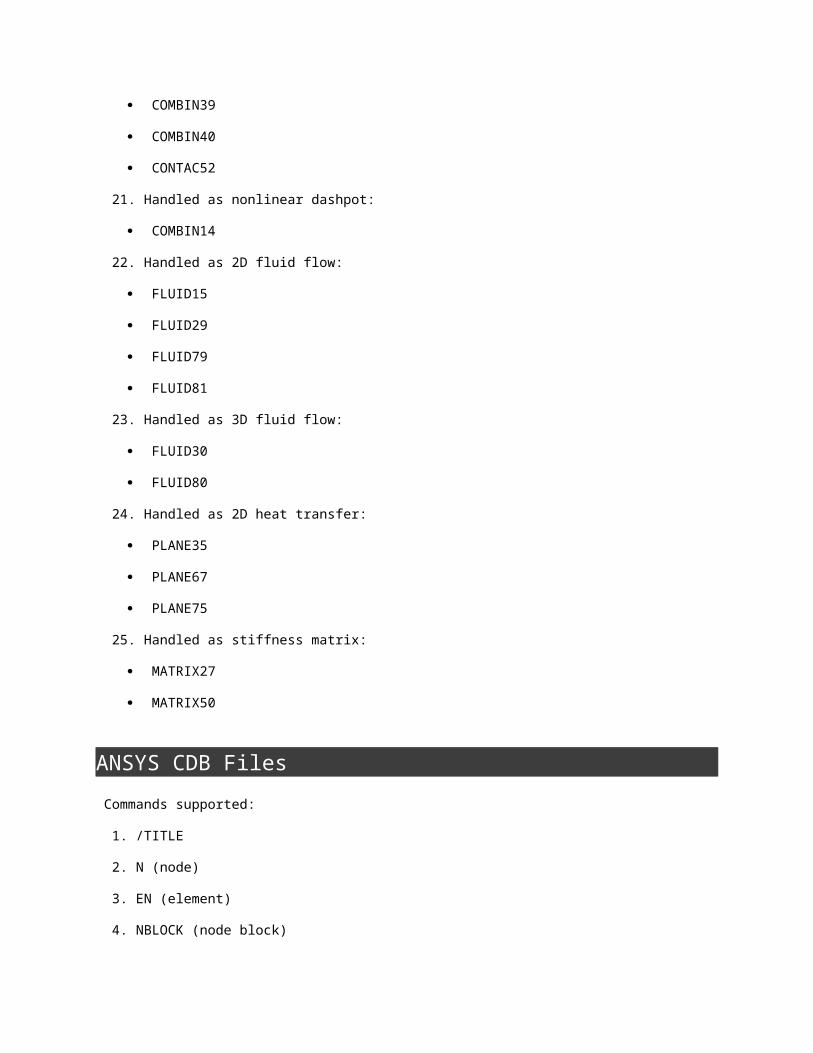
20. Handled as nonlinear general contact:

COMBIN7

CONTAC12

CONTAC26

COMBIN37

COMBIN39

COMBIN40

CONTAC52

21. Handled as nonlinear dashpot:

COMBIN14

22. Handled as 2D fluid flow:

FLUID15

FLUID29

FLUID79

FLUID81

23. Handled as 3D fluid flow:

FLUID30

FLUID80

24. Handled as 2D heat transfer:

PLANE35

PLANE67

PLANE75

25. Handled as stiffness matrix:

MATRIX27

MATRIX50

ANSYS CDB Files Commands supported:

1. /TITLE

2. N (node)

3. EN (element)

4. NBLOCK (node block)

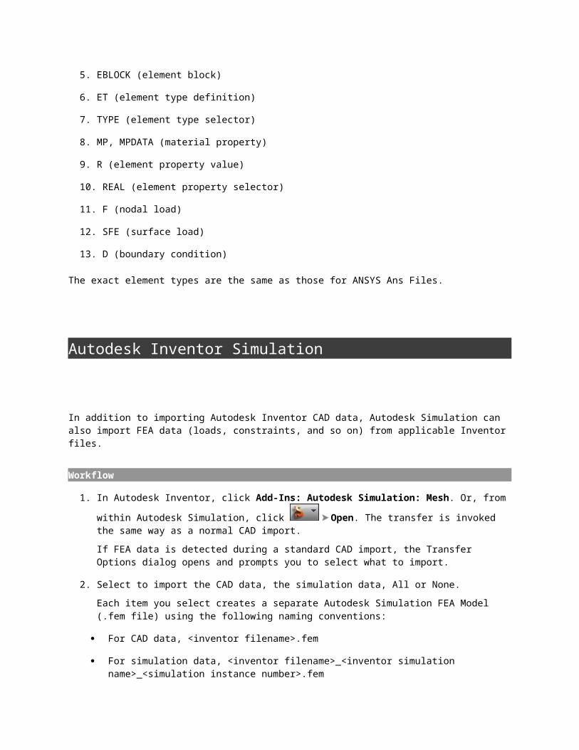
5. EBLOCK (element block)

6. ET (element type definition)

7. TYPE (element type selector)

8. MP, MPDATA (material property)

9. R (element property value)

10. REAL (element property selector)

11. F (nodal load)

12. SFE (surface load)

13. D (boundary condition)

The exact element types are the same as those for ANSYS Ans Files.

Autodesk Inventor Simulation

In addition to importing Autodesk Inventor CAD data, Autodesk Simulation can also import FEA data (loads, constraints, and so on) from applicable Inventor files.

Workflow

1. In Autodesk Inventor, click Add-Ins: Autodesk Simulation: Mesh. Or, from within Autodesk Simulation, click Open. The transfer is invoked the same way as a normal CAD import. If FEA data is detected during a standard CAD import, the Transfer Options dialog opens and prompts you to select what to import.

2. Select to import the CAD data, the simulation data, All or None. Each item you select creates a separate Autodesk Simulation FEA Model (.fem file) using the following naming conventions:

For CAD data, <inventor filename>.fem

For simulation data, <inventor filename>_<inventor simulation name>_<simulation instance number>.fem

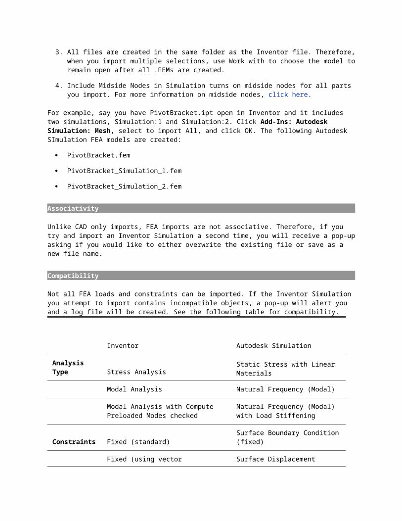
3. All files are created in the same folder as the Inventor file. Therefore, when you import multiple selections, use Work with to choose the model to remain open after all .FEMs are created.

4. Include Midside Nodes in Simulation turns on midside nodes for all parts you import. For more information on midside nodes, click here.

For example, say you have PivotBracket.ipt open in Inventor and it includes two simulations, Simulation:1 and Simulation:2. Click Add-Ins: Autodesk Simulation: Mesh, select to import All, and click OK. The following Autodesk SImulation FEA models are created:

PivotBracket.fem

PivotBracket_Simulation_1.fem

PivotBracket_Simulation_2.fem

Associativity

Unlike CAD only imports, FEA imports are not associative. Therefore, if you try and import an Inventor Simulation a second time, you will receive a pop-up asking if you would like to either overwrite the existing file or save as a new file name.

Compatibility

Not all FEA loads and constraints can be imported. If the Inventor Simulation you attempt to import contains incompatible objects, a pop-up will alert you and a log file will be created. See the following table for compatibility.

Inventor Autodesk Simulation

Analysis Type Stress Analysis

Static Stress with Linear Materials

Modal Analysis Natural Frequency (Modal)

Modal Analysis with Compute Preloaded Modes checked

Natural Frequency (Modal) with Load Stiffening

Constraints Fixed (standard) Surface Boundary Condition (fixed)

Fixed (using vector components) Surface Displacement Boundary

Pin Pin Constraint

Frictionless Requires future development

Loads Force Surface Force 1

Pressure Surface Pressure 1

Bearing Requires future development

Gravity Gravity / Acceleration

Moment Requires future development

Remote Force Requires future development

Body Load Gravity / Acceleration 2 or Centrifugal

Contact Bonded Bonded

Separation Surface

Sliding / No Separation Sliding / No Separation Contact

Separation / No Sliding Separation / No Sliding Contact

Shrink fit / sliding Requires future development

Shrink fit / no sliding Requires future development

Spring (user-defined stiffness) Requires future development

1 maximum of one surface force or surface pressure per surface.

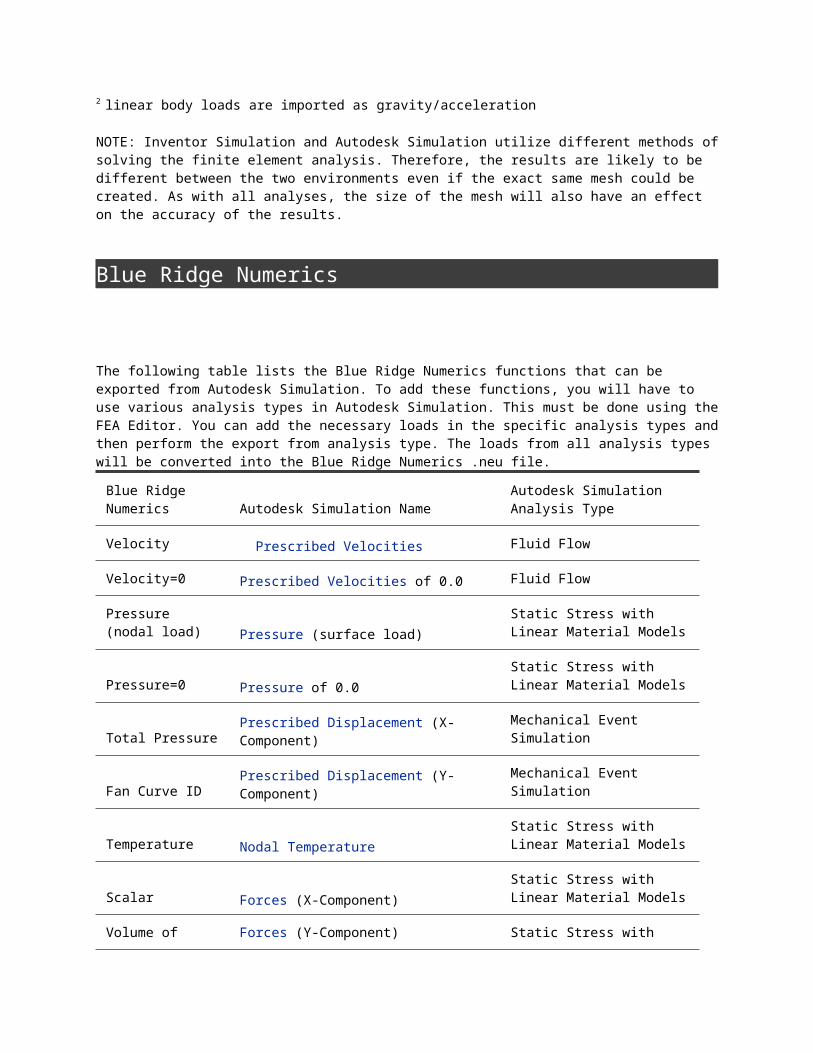
2 linear body loads are imported as gravity/acceleration

NOTE: Inventor Simulation and Autodesk Simulation utilize different methods of solving the finite element analysis. Therefore, the results are likely to be different between the two environments even if the exact same mesh could be created. As with all analyses, the size of the mesh will also have an effect on the accuracy of the results.

Blue Ridge Numerics

The following table lists the Blue Ridge Numerics functions that can be exported from Autodesk Simulation. To add these functions, you will have to use various analysis types in Autodesk Simulation. This must be done using the FEA Editor. You can add the necessary loads in the specific analysis types and then perform the export from analysis type. The loads from all analysis types will be converted into the Blue Ridge Numerics .neu file.

Blue Ridge Numerics Autodesk Simulation Name

Autodesk Simulation Analysis Type

Velocity Prescribed Velocities Fluid Flow

Velocity=0 Prescribed Velocities of 0.0 Fluid Flow

Pressure (nodal load) Pressure (surface load)

Static Stress with Linear Material Models

Pressure=0 Pressure of 0.0 Static Stress with Linear Material Models

Total PressurePrescribed Displacement (X-Component)

Mechanical Event Simulation

Fan Curve IDPrescribed Displacement (Y-Component)


Temperature Nodal Temperature Static Stress with Linear Material Models

Scalar Forces (X-Component) Static Stress with Linear Material Models

Volume of Fluid Forces (Y-Component) Static Stress with Linear Material Models

Unknown Inlet/Outlet

Prescribed Rotation (Y-Component) Non-zero


Slip WallPrescribed Rotation (Z-Component) Non-zero


Heat Source Internal Heat Generation Heat Transfer

Nodal Heat Source Applied Temperature Heat Transfer

Heat Flux Heat Flux Heat Transfer

Surface Radiation

Radiation (Radiation Function and Temperature) Y and X Heat Transfer

Film CoefficientsConvection (Coefficient and Temperature) Y and X Heat Transfer

Periodic Wall Moments (X-Component)(1, 2, or 3) Static Stress with Linear Material Models

FEMAP

Data blocks supported:

1. 100 (header)

2. 601 (materials)

3. 402 (properties)

4. 403 (nodes)

5. 404 (elements)

6. 506 (constraints)

7. 507 (loads)

8. 412 (active data)

9. 433, 533 (min/max)


1. Handled as trusses:

1 (rods)

29 (rigid)

2. Handled as beams:

2 (bars)

3 (tubes)

4 (links)

5 (beams)

8 (curved beams)

3. Handled as bricks:

25, 26 (solids)

4. Handled as membranes:

11, 12 (shear)

13, 14 (membrane)

15, 16 (bending)

5. Handled as plates:

17, 18 (plates)

6. Handled as boundary elements:

6 (springs)

7 (DOF springs)

7. Handled as gap/cable elements:

9 (gap)

8. Handled as 2D elements:

19, 20 (plane strain)

23, 24 (axisymmetric)

9. Handled as composite elements:

21, 22 (laminates)

The geometry types which are supported are:

1. 0 (lines)

2. 2 (3-noded triangles)

3. 3 (6-noded triangles)

4. 4 (4-noded quads)

5. 5 (8-noded quads)

6. 6 (4-noded tets)

7. 7 (6-noded wedges)

8. 8 (8-noded bricks)

9. 10 (10-noded tets)

10. 11 (15-noded wedges)

11. 12 (20-noded bricks)

NASTRAN

Autodesk Simulation will import and export models in the MSC.Nastran format.

Static stress with linear material models:

The following table explains how each NASTRAN item is handled when it is transferred. This table can be reversed for information on how Autodesk Simulation items are translated to the NASTRAN input file with the exceptions listed below the table.

NASTRAN Autodesk Simulation

Truss Elements PROD/CROD or CONROD Linear truss

Beam Elements PBAR/CBAR

Linear beam (offsets and end releases will also be transferred from CBAR)

PLOAD1 Linear beam distributed loads

PBEAM/CBEAM

Linear beam with constant cross-sectional properties (the first set of cross-sectional properties will be used)

Gap Elements PGAP/CGAP Gap element

Plate Elements

PSHELL/CQUAD4/CQUADR/CTRIA3/ CTRIAR with values in the MID1 and MID2 fields

Linear plate (material properties will depend on the MAT type as described below)

PSHELL/CQUAD8/CTRIA6 with values in the MID1 and MID2 fields

Linear plate (midside nodes will not be translated)

MAT1 Isotropic material model

MAT2 If the material is orthotropic material model, an orthotropic material model will be used; if the material is anisotropic, no

material properties will be translated

MAT8 Orthotropic material model

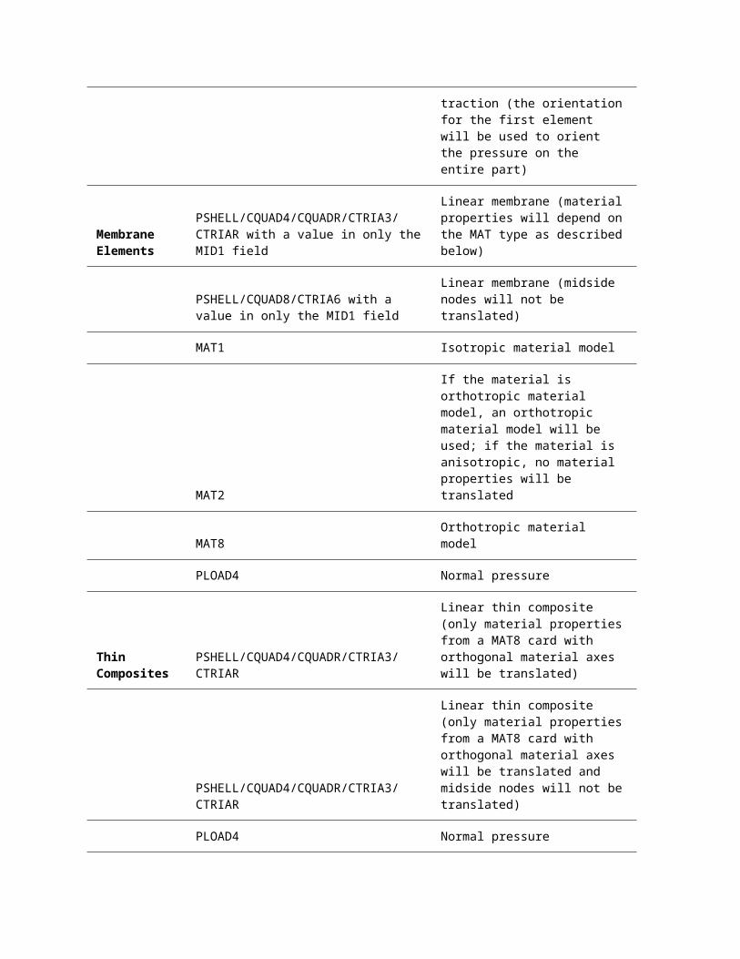
PLOAD4

Normal pressure or traction (the orientation for the first element will be used to orient the pressure on the entire part)

Membrane Elements

PSHELL/CQUAD4/CQUADR/CTRIA3/ CTRIAR with a value in only the MID1 field

Linear membrane (material properties will depend on the MAT type as described below)

PSHELL/CQUAD8/CTRIA6 with a value in only the MID1 field

Linear membrane (midside nodes will not be translated)


MAT2

If the material is orthotropic material model, an orthotropic material model will be used; if the material is anisotropic, no material properties will be translated


PLOAD4 Normal pressure

Thin Composites

PSHELL/CQUAD4/CQUADR/CTRIA3/ CTRIAR

Linear thin composite (only material properties from a MAT8 card with orthogonal material axes will be translated)


Linear thin composite (only material properties from a MAT8 card with orthogonal material axes will be translated and midside nodes will not be translated)


Brick PSOLID/CHEXA/CPENTA/CTETRA Linear brick (material properties will depend on the MAT type as described below, if all the midside nodes are present, they will be translated, if one of the midside nodes are not

present, no midside nodes will be translated)


MAT9


MATT1Temperature dependent isotropic

MATT9



Rigid Elements RBE2 Rigid element

Other Element Types PSHEAR/CSHEAR

The CSHEAR element and properties are imported as if they are PSHELL and CQUAD4 cards.

Nodal Loads and Constraints FORCE Nodal force

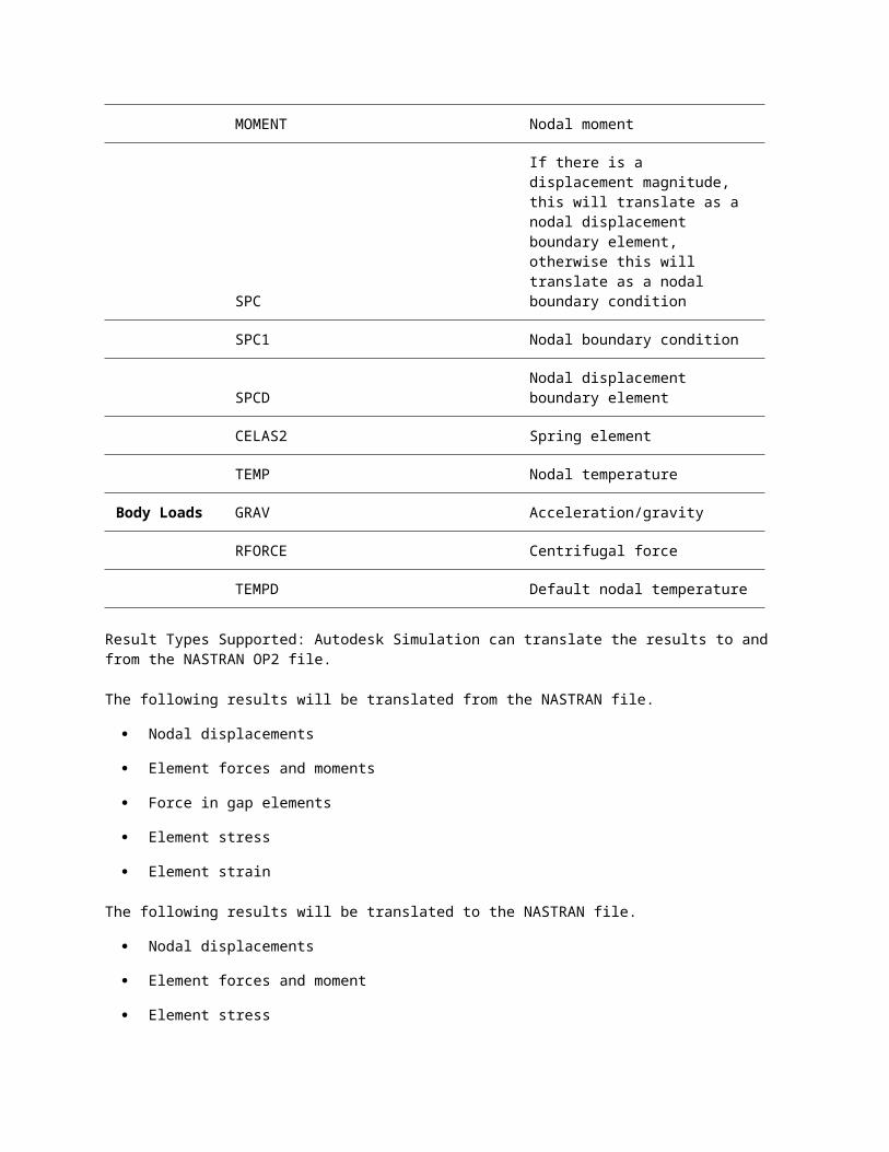
MOMENT Nodal moment

SPC

If there is a displacement magnitude, this will translate as a nodal displacement boundary element, otherwise this will translate as a nodal boundary condition

SPC1 Nodal boundary condition

SPCDNodal displacement boundary element

CELAS2 Spring element

TEMP Nodal temperature

Body Loads GRAV Acceleration/gravity

RFORCE Centrifugal force

TEMPD Default nodal temperature

Result Types Supported: Autodesk Simulation can translate the results to and from the NASTRAN OP2 file.

The following results will be translated from the NASTRAN file.

Nodal displacements

Element forces and moments

Force in gap elements

Element stress

Element strain

The following results will be translated to the NASTRAN file.

Nodal displacements

Element forces and moment

Element stress

Element strain

Composite results

Steady-state heat transfer



Rod Elements PROD/CROD or CONROD Thermal rod


MATT4Isotropic temperature-dependent material model

Plate Elements


Thermal plate (material properties will depend on the

MAT type as described below)


MATT4Temperature-dependent isotropic material model


MATT5Temperature-dependent orthotropic material model

Brick PSOLID/CHEXA/CPENTA/CTETRA

Thermal brick (material properties will depend on the MAT type as described below)



MATT5Temperature-dependent orthotropic

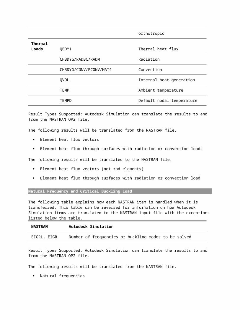
Thermal Loads QBDY1 Thermal heat flux

CHBDYG/RADBC/RADM Radiation

CHBDYG/CONV/PCONV/MAT4 Convection

QVOL Internal heat generation

TEMP Ambient temperature

TEMPD Default nodal temperature



Element heat flux vectors

Element heat flux through surfaces with radiation or convection loads

The following results will be translated to the NASTRAN file.

Element heat flux vectors (not rod elements)

Element heat flux through surfaces with radiation or convection load

Natural Frequency and Critical Buckling Load



EIGRL, EIGR Number of frequencies or buckling modes to be solved



Natural frequencies

Mode shapes

Buckling multipliers

In most cases, items in Autodesk Simulation will be translated to NASTRAN. There are a few exceptions:

If a brick model in Autodesk Simulation contains pyramids (5-noded elements), they will be split into 2 tetrahedral elements when translated to NASTRAN. This will also occur if a model is solved in Autodesk Simulation using the NASTRAN solver.

2D elements are not supported by NASTRAN. When translated to NASTRAN, the geometry, material properties and loads will be translated to PSHELL/CQUAD4.

Thick Composite elements are not supported by NASTRAN. When translated to NASTRAN, the geometry, material properties and loads will be translated to PCOMP/CQUAD4. Any core crushing properties will not be translated.

Rigid boundary elements will be translated as CELAS2 in NASTRAN.

A spring element will be translated as CONROD in NASTRAN. A DOF spring element will be translated as CELAS2 in NASTRAN.

Local coordinate systems will be translated to CORD2R, CORD2C and CORD2S in NASTRAN.

If a model contains linear contact, the contact elements will be translated to PGAP and CGAP cards. A rectangular coordinate system will also be created for each element to define the axial direction.

If a model contains thermal contact, the thermal contact elements will not be exported.

PATRAN Packet types supported:

1. 01 (Node Data)

2. 02 (Element Data)

3. 03 (Material Properties)

4. 04 (Element Properties)

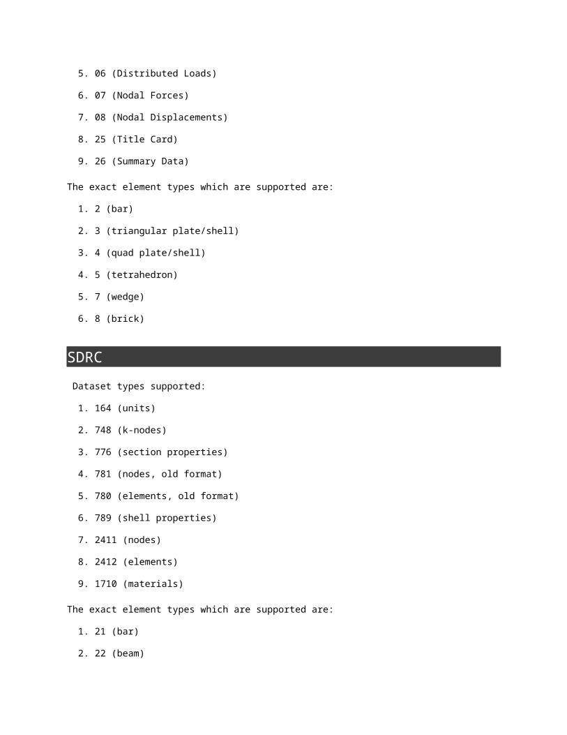
5. 06 (Distributed Loads)

6. 07 (Nodal Forces)

7. 08 (Nodal Displacements)

8. 25 (Title Card)

9. 26 (Summary Data)


1. 2 (bar)

2. 3 (triangular plate/shell)

3. 4 (quad plate/shell)

4. 5 (tetrahedron)

5. 7 (wedge)

6. 8 (brick)

SDRC Dataset types supported:

1. 164 (units)

2. 748 (k-nodes)

3. 776 (section properties)

4. 781 (nodes, old format)

5. 780 (elements, old format)

6. 789 (shell properties)

7. 2411 (nodes)

8. 2412 (elements)

9. 1710 (materials)


1. 21 (bar)

2. 22 (beam)

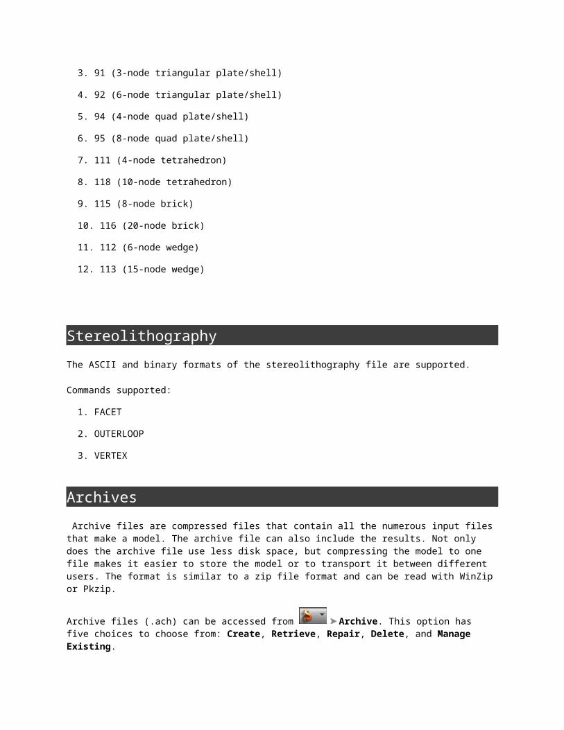
3. 91 (3-node triangular plate/shell)

4. 92 (6-node triangular plate/shell)

5. 94 (4-node quad plate/shell)

6. 95 (8-node quad plate/shell)

7. 111 (4-node tetrahedron)

8. 118 (10-node tetrahedron)

9. 115 (8-node brick)

10. 116 (20-node brick)

11. 112 (6-node wedge)

12. 113 (15-node wedge)

Stereolithography The ASCII and binary formats of the stereolithography file are supported.

Commands supported:

1. FACET

2. OUTERLOOP

3. VERTEX

Archives Archive files are compressed files that contain all the numerous input files that make a model. The archive file can also include the results. Not only does the archive file use less disk space, but compressing the model to one file makes it easier to store the model or to transport it between different users. The format is similar to a zip file format and can be read with WinZip or Pkzip.

Archive files (.ach) can be accessed from Archive. This option has five choices to choose from: Create, Retrieve, Repair, Delete, and Manage Existing.

Create command

The create option will allow you to create a file with a .ach extension. When you select the Create command the Archive Creation Options dialog will appear:

You can choose between Model only and Model and results. Once you press the OK button, a compressed file with the .ach extension will be made. This makes it so only one file is needed to archive. This is a good way to back up a model. Also, it is very useful to keep a record of your model. The .ach file is the only file needed to open your model.

The Model only option will only include the loads, geometry, element data, material data, global data, and any other input data (.fem file and input stored under the modelname.ds_data folder.) Pre-meshed wireframes, previous versions, or result files are not included. The Model and results option will include every file in the current directory with the model name and all files under the modelname.ds_data folder. This will include pre-meshed wireframes, result files, log files, screen captures (if they were named the same as the model name), and meshing result files. Both options include all the design scenarios in the model.

The archive only includes files related directly to the current model. If any of the design scenarios access results from a different model (a file with a different name), those external results are not included in the archive. Therefore, the other model or models should be archived also.

The archive utility can handle approximately 2^64 number of files and 2^64 bytes per file, both of which are beyond realistic capabilities with current software and hardware.

If you are having an analysis-related problem that you need to send to Technical Support, archive the model with results. If the archive file is too large to send via e-mail, archive the model without results and attach the processor log files that will include the error messages so that we will know exactly where to focus on your model.

Retrieve command

If you select the Retrieve command, you can retrieve an existing archive file. This will let you unzip the archive file and display the model in Autodesk Simulation so that you can make changes to it. For example, you will need to use this option to retrieve the verification examples from the AVE Manual. NoteDue to limitations in Windows with long paths, archives should not be retrieved to folders with excessively long names. For more information, see the Introduction.

Manage Existing command

Use the Manage Existing command to see and manage an existing archive file. The dialog lists all the files in the archive file. Remove or update any file.

Repair command

If an archive file has become corrupt you can use the Repair command to fix it.

Delete command

The Delete command will bring up a dialog where you can select an archive file. The selected archive file will then be deleted. NoteIf the archive utility gives a message like Component ‘XceedZip.dll’ or one of its dependencies not correctly registered: a file is missing or invalid, then run the batch file

regall.bat located in the Autodesk Simulation installation folder. (See the paragraph General Troubleshooting on the page Installation Guide: CAD Setup and Troubleshooting for details on running regall.bat.)

Open Model Files from CDs If Models are in an archive (.ach) Format:

Copy the archive file to the hard disk.

Start Autodesk Simulation.

Use the Archive Retrieve command to open the model.

If Models are not in an Archive Format:

When files are copied from a CD to the hard disk, the files may be marked as read only. (It depends on the operating system.) Trying to open a model that is read only will cause an error message. In these situations, the following steps need to be done.

Copy all the files for the model, including the .ds_data folder, to the hard disk.

Using My Computer or Windows Explorer, highlight all the files and folders for the model on the hard disk.

Right-click one of the files and choose the Properties command.

Deactivate the Read-only check box. Apply the changes to all subfolders and files.

The model is now ready to be opened.

After You Open a Model After opening the model, there are two major steps left before running an analysis:

1. Mesh the model. See the page Meshing Overview.

2. Apply loads, constraints, element and material properties. See the page Setting Up and Performing the Analysis.

Mesh Models

Topics in this section Mesh Overview

Mesh Overview You can mesh in many ways in the FEA Editor environment.

Create solid, midplane, or surface meshes automatically from CAD solid models.

Draw and automatically mesh 2D sketches that enclose a region. Although the planar automatic mesh is limited to sketches in a plane, the plane can be at any orientation. Use these meshes for 2D elements or plate-like meshes.

Create structured meshes from corner nodes or between sketch objects.

Create additional meshes for the previously mentioned ones. Select, copy, extrude or modify lines to create additional meshes. For example, imagine a 2D sketch that is meshed to give a flat plate. If the edge of the mesh is selected and extruded, a box is created (such as a pressure vessel or tank). If the entire mesh is selected and extruded, a solid mesh is created.

Construct line element models, such as beam or truss element models, or add line elements to geometry created by any other method.

Topics in this section Meshing CAD Solid Models Create and Modify Geometry in the FEA Editor Meshing Hand-built Models Surface Mesh Enhancing PVDesigner Contact Pairs Transition from Superdraw III to Autodesk Simulation

Meshing CAD Solid Models A good mesh is the balance of precision and computation time. Quality meshes converge quickly, produce accurate results and do not produce errors. The majority of the meshing process involves the mesh settings.

Topics in this section Meshing Process Model Mesh Settings

Mesh Results Watertight Problems in Meshes Feature Matching Joint components Bolts and other fasteners Refinement Points Construction Vertices - Seed Points Fluid Generation Perform Mesh Studies

Meshing Process

Get a good surface mesh because it controls the quality of the solid mesh.

Meshing basics

1. Open the solid model.

2. On the Model Mesh Settings dialog box, select the appropriate option in the Mesh type section for the model.

Select Solid if the model will be analyzed using brick elements.

Select Midplane if the model is a 3D solid model but will be analyzed using plate or shell elements. The solid part collapses down to plate elements at the midplane.

Select Plate/shell if the model already consists of only surfaces and will be analyzed as plate or shell elements.

If the part is a gasket element type (nonlinear stress analysis), click the part in the tree view set the element type to 3D Gasket.

3. Click Mesh model. (Or use Mesh Mesh Generate 3D Mesh.)

4. After the meshing process completes, click Yes to view the results of the mesh.

If the results are not acceptable, adjust the mesh size with one of these techniques:

On the Mesh Mesh 3D Mesh Settings dialog box, move the Mesh size slider towards Coarse or Fine and click Mesh Model again to create a new mesh.

If a finer mesh is required around closely spaced features, select the Mesh Refinement Points Automatic command.

Move the slider to the appropriate position and press Generate. Black refinement points are added to the model. Move the slider and click Generate again to change

the number of refinements. Click Done after the appropriate number of refinement points are created. Use Mesh Mesh Generate 3D Mesh to create a new mesh.

Meshing of a CAD model is a two or three step process when generating a solid mesh. First, the surface of the CAD model is meshed (Surface meshing Part n shown in the progress dialog). After all parts are surface meshed, the surface mesh is verified to ensure that each part is properly meshed, meaning that the mesh on each face matches the adjoining face, and thereby creating a watertight solid (Verifying surface mesh for Part n). Finally, the solid mesh is created to fill the volume of each part with solid elements (Solid meshing Part n). Depending on the option chosen under Mesh Mesh 3D Mesh Settings Options Model, the solid mesh can be delayed until the analysis is started or performed immediately after generating the surface mesh. NoteIn a multi-part assembly, the parts are meshed in order of smallest to largest volume. They are not meshed in numerical order. So the Information section of the Meshing Progress dialog may indicate that it is Surface meshing part 101 while the progress indicates Part 5 of 314.

When loads or boundary conditions are existing in the model and the model is re-meshed, the following will occur:

Surface based loads and surface based conditions will be maintained.

Edge loads and edge boundary conditions will be maintained.

Nodal loads and nodal boundary conditions must be re-applied to the model. Important

After generating the mesh, you can change the attributes of the lines (part, surface, and layer) for specific requirements. For example, it may be advantageous to combine multiple surfaces into one surface number to make it easier to apply and modify a load. Be aware that some manual changes may be overwritten if the CAD part is remeshed and some are not. In particular:

If the lines are changed to a different part number (not a CAD part), the modified lines will remain when the CAD part is remeshed.

If the lines are changed to a different surface number within the same part, then:

if the lines are placed on a surface number that does not exist in the CAD part, the modified lines will remain when the CAD part is remeshed. Be careful that the modified lines do not create a problem with the CAD model. That is, it may be necessary to manually select and delete the modified lines.

if the lines are placed on a surface number that exists in the CAD part, the modified lines will be overwritten when the CAD part is remeshed.

If the lines are changed to a different layer number within the same part, the modified lines will be overwritten when the CAD part is remeshed.

In addition to the steps presented above, different situations may require some extra steps. This section presents some of the more common advanced features of meshing CAD solid models (in no particular order).

General tips

In a multi-part assembly, all of the activated parts are meshed when the Generate Mesh command is used. This ensures that matching of meshes occurs between mating parts. If for some unusual reason you do not want to mesh the entire model and are not concerned with the matching of the mesh, then deactivate all of the parts that you do not want to mesh (select, right-click, and choose Deactivate). Any existing meshes on the deactivated parts will not be changed.

In some cases, a node is required at a specific location. To do this, add a construction vertex (formerly known as a seed point). After generating an initial surface mesh, select a vertex ( Selection Select Vertices ) in the area of and at a known position relative to the desired construction vertex, right-click, and choose Add Construction Vertices. Enter the offset DX DY DZ from the selected vertex for the construction node. See also the page Construction Vertices -Seed Points.

If working with an assembly of parts and want a different type of mesh on different parts (bricks and plate elements), right-click that part in the display area or the tree view and select the CAD Mesh Options Part command. This will access a screen identical to the screen accessed by Mesh Mesh 3D Mesh Settings but these mesh settings will only be applied to the selected part. Then choose the desired Mesh type.

Mesh size

In addition to using the slider on the Model Mesh Settings screen to set the mesh size based on an arbitrary percentage, clicking the Options button and setting the Mesh size: Type to Absolute mesh size will allow the mesh size to be entered as an actual dimension.

If working with an assembly of parts, different mesh sizes can be used for each part. Right-click that part in the display area or the tree view and select the CAD Mesh Options Part command. This will access a screen identical to the screen accessed by Mesh Mesh 3D Mesh Settings but these mesh settings will only be applied to the selected part. If you have specified part mesh settings for some parts in a model and want to mesh the entire model with the model mesh settings, use Mesh Mesh All Parts Use Model Settings. If you have specified part mesh settings for some parts in a model and want to mesh one of them with the model mesh settings, right-click that part in the display area or tree view and select the CAD Mesh Options

Model command.

NoteWhen a part is assigned to the Part mesh settings, the symbol in the tree-view changes from (Model Mesh Settings) to . When using the Use automatic geometry-based mesh size function (set under Mesh Mesh 3D Mesh Settings Options Model), the mesh size created when using Percent of automatic is different in each part (based on the part's physical size). Use the Part mesh settings to further control the mesh size of individual parts.

In addition to the automatic refinement point capabilities described above, user specified refinement points can be created using one of these techniques. See also the page Refinement Points.

After creating an initial surface mesh, select vertices (Selection Select Vertices), right-click, and choose Add Refinement Points. Enter the refined mesh size and radius around the refinement point in which mesh is to be refined.

If the coordinates of the desired refinement point are known, the refinement points can be added before meshing the model by using Mesh Refinement Points Specify.

Small elements around curved features can be created by adjusting the parameters in the Edge curve refinement section of the Options tab of the Mesh Mesh 3D Mesh Settings Options Surface dialog. (See the page Meshing Overview: Meshing CAD Solid Models: Model Mesh Settings: Surface for details.)

Contact and mesh matching between parts

When meshing assemblies where the meshes on the mating parts must be matched up, (to transfer a load from one part to another), use approximately (if not exactly) the same mesh size for both parts. This will assure a good match between the meshes of these parts.

Small gaps between parts, whether intentional or not, can behave unexpectedly. When unintentional, the gap may prevent the meshes from being matched between mating parts. (Keep in mind that all numbers are subjected to round off, so even a perfect CAD model may have a mathematical gap between parts.) Or perhaps a small intentional gap between parts is removed when the model is meshed; that is, the parts are stretched to mate the parts. How far to stretch the mesh is controlled by the mesh matching tolerance. See the page Meshing Overview: Meshing CAD Solid Models: Model Mesh Settings: Model.

The mesh around the perimeter where two parts match may be smoother if the parts are knitted when the CAD solid model is opened into Autodesk Simulation. See the page Opening Models: Opening CAD Files: Surface Knitting.

The type of contact between two mating parts can be set using the Contact entry at the bottom of the tree view. Contact can be set for the entire model with this tree view entry. Or contact between two parts, or even between individual surfaces can be set by selecting those items, right-click, and choosing Contact. The types of contact available depend on the analysis type. See also the page Creating Contact Pairs.

If performing a Mechanical Event Simulation (MES) analysis with surface-to-surface contact, and if the parts are starting in contact but will slide or separate, you should not have the meshes matched on the surfaces that will be involved in contact if possible. This condition can lead to poor convergence (longer runtime). To prevent the meshes from matching, use the Prevent part matching option on the Model Mesh Settings dialog. (See the page Meshing Overview: Meshing CAD Solid Models: Model Mesh Settings: Model.) On the other hand, if the parts are initially in contact and the sliding motion is negligible, then the meshes can be matched; specify Point-to-point as the contact type in this situation.

Solid meshing

If generating a solid mesh, there are numerous options for the type of solid mesh (hybrid of bricks, all tetrahedral, and so on.) From the Mesh Mesh 3D Mesh Settings dialog, click the Options button, and then click Solid to view the types of solid mesh on the General tab. See also the page Model Mesh Settings: Solid.

Thin parts

If your part is thin (one element through the thickness), consider using the Midplane option to generate plate mesh instead of a brick mesh. (Plate elements treat bending more accurately than one brick element through the thickness.) Another option would be to use the Bricks and wedges (layered mesh of thin parts) option for a solid mesh. This option creates a solid mesh with a user number of brick elements through the thickness. See also the page Model Mesh Settings: Solid.

Fluid flow analysis and multiphysics analysis

If performing a fluid analysis, keep in mind that the fluid volume needs to be meshed. If the CAD model is of the solid parts, you may be able to generate the fluid volume by using the Mesh: Fluid Generation command.

Fluid models often require a finer mesh near the wall than at the center of the volume to capture the wall effects. Use the Tetrahedra and wedges (boundary layer) option to produce a thin layer of elements at the wall. See the paragraph Controlling Boundary Layer Meshes on the page Meshing Overview: Meshing CAD Solid Models: Model Mesh Settings: Solid.

If the boundary layer mesh is not used, then the solid mesh type will default to All tetrahedra for new fluid models. This option results in the best results for fluid models. (Multiphysics analysis uses the All tetrahedra mesh type for all parts so that the faces match between the fluid parts and the solid parts.) See the paragraph Selecting a Mesh Type on the page Meshing Overview: Meshing CAD Solid Models: Model Mesh Settings: Solid. (The solid mesh type on existing models will not be changed to All tetrahedra if the model is remeshed.)

Gasket materials

If one of the parts of the model is destined to be a gasket, then set the element type to 3D Gasket before creating the mesh. This will instruct the mesh engine to generate only one element through the thickness: one of the requirements of the gasket element. See also 3D Gasket Elements. When a part is assigned to the Gasket mesh settings, the symbol in the tree-view changes to a part mesh setting . The gasket setting is also accessible by selecting the part, right-clicking and choosing CAD Mesh Options Part Options Solid

Gasket.

Model Mesh Settings

Use the Mesh Mesh 3D Mesh Settings dialog box to mesh a CAD solid model in the FEA Editor environment. It sets the mesh settings for all the parts in the model. An identical screen appears when you specify the mesh settings for a single part in the model. (Select a part or multiple parts in the tree view, right-click, and select CAD Mesh Options Part.)

Mesh type section

Solid: Selected parts are meshed with solid elements (brick or tetrahedral).

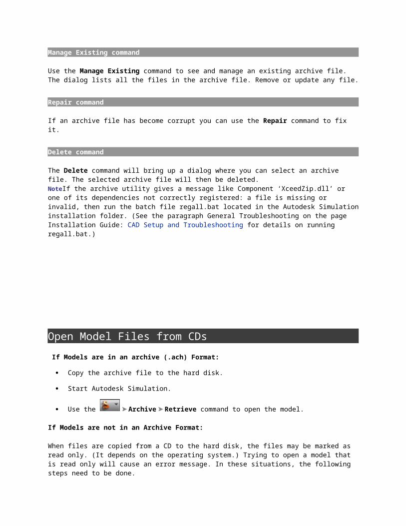
Midplane: Select if the selected parts are solid parts but will be collapsed to the midplane of the solid parts. After creating the midplane mesh, the average thickness of the plate elements is automatically used as the thickness for each surface. To use a specific value (for either the entire part or different surfaces within the part), clear the Use mid-plane mesh thickness check box in the Element Definition screen for the part.

Plate/shell: Select if the selected parts are surfaces for example, have no modeled thickness. The difference between the three types of mesh (solid, midplane, and plate/shell) are demonstrated in the following images of two intersecting pipes. The figures show the model sliced in half, and the elements are shrunk to reveal the elements. Solid mesh: The volume between the inside surface and the outside surface of the CAD model is filled with brick elements. The thickness does not need to be entered. It is based on the mesh.

Midplane mesh: The inside surface and the outside surface of the CAD model are collapsed to the midplane location, and the mesh is created at the midplane. The thickness of the solid is represented by entering a numerical value (in the Element Definition) for the thickness of the elements. (The elements can be any type of area elements, such as plate elements or membrane elements.)

Plate/shell mesh: All surfaces of the CAD model, the inside surface and the outside surface, are meshed. The thickness of each element is represented by entering a numerical value (in the Element Definition). Unless you intended to create a double-walled vessel, this type of mesh is incorrect for this example CAD model. In this analysis, the two surfaces can move independently and pass through each other.

Options: You can specify further mesh settings for the selected parts. Surface Solid Midplane Model

Control the mesh size

This slider in the Mesh size section controls the size of the mesh on the selected parts relative to the default size which is calculated based on the model dimensions.

Defaults button

Access the Meshing Option Defaults dialog box.

Mesh model button

The model is meshed with the current settings. This button will only be available if you are specifying the settings for the entire model.

NoteIn a multi-part assembly, the parts are meshed in order of smallest to largest volume. They are not meshed in numerical order. So the Information section of the Meshing Progress dialog may indicate that it is Surface meshing part 101 while the progress indicates Part 5 of 314.

Topics in this section Surface Solid Midplane Model

Mesh Size Hints To get the best mesh possible on a CAD solid model, it is suggested to set the

mesh size to the smallest diameter in your model divided by four. The mesh size should be smaller than the smallest radius of curvature or feature to

be modeled. The easiest way to check the mesh size is to look at the edges of small circular holes in the feature file. Each circle should be divided into at least 5 or 6 segments.

Figure 1 shows the features of a model that was meshed using an appropriate size mesh. Note that the small red hole on the bottom right has its circumference divided into 6 sections.

Figure 1: Features of a Model with an Appropriate Mesh Size Figure 2 shows the features of a model that was meshed using a mesh size that

was too large. Note that the small red hole on the bottom right has its circumference divided into 4 sections.

Figure 2: Features of a Model with a Too Large Mesh Size Figure 3 shows the features of a model that was meshed using a mesh size that

was much too large. Note that the small red hole on the bottom right has been flattened.

Figure 3: Features of a Model with a Much Too Large Mesh Size

Solid

When the Options button is pressed on the Model Mesh Settings screen or Part Mesh Settings screen and the Solid icon is selected, a screen with multiple tabs will appear. (Note: The Solid icon will only be present if the Solid radio button is selected in the Mesh type section of the Model Mesh Settings screen.) Click the link for the subject that you need more information about.

Select a mesh type

The mesh types can be selected in the Solid mesh type section of the General tab. The options are as follows:

Bricks and tetrahedra: The solid mesh will consist of as many 8-node brick elements as possible with respect to the mesh size. When necessary toward the center of the model, 6-node wedge, 5-node pyramid or 4-mode tetrahedral elements may be created. The majority of the volume will consist of 8-node elements. This option will create the highest quality mesh with the fewest elements.

All tetrahedra: The solid mesh will consist of all 4-node tetrahedral elements. The main purpose of this mesh type is for fluid flow analysis. If not using the boundary layer mesh described below, then the mesh should be an all tetrahedra mesh for fluid flow and multiphysics analyses. (Multiphysics analysis uses the All tetrahedra mesh type for all parts so that the faces match between the fluid parts and the solid parts.) (Technically, an all brick mesh would be required if using the Penalty formulation. But since the Penalty formulation is optimal only for very small model sizes, it is rarely encountered with a mesh derived from a CAD solid model.) For other analysis types, this option will require significantly more elements to get the same accuracy as the Bricks and tetrahedra option.

All bricks: The solid mesh will consist of all 8-node brick elements. To achieve this solid mesh, the surface mesh may be meshed finer than the mesh size setting would imply. This in turn will create many more elements than the Bricks and tetrahedra option, and should only be used when necessary. Since the Autodesk Simulation processors handle all types of solid elements, this option is not necessary when working with the Autodesk Simulation solvers.

Tetrahedra and wedges (boundary layer): A special mesh of boundary layer elements will be created at all surfaces of the part using 6-node wedge elements. Then, the solid mesh will consist of 4-node tetrahedral elements. This type of mesh is often used for fluid flow models.

Bricks and wedges (layered mesh of thin parts): This mesh will create a user-entered number of solid elements through the thickness. Since the number through the thickness is applied throughout the part, this option is suitable for thin parts with relatively constant thickness. Note that although thin part meshing of multiple part assemblies is possible, the mesh may not be matched on parts that are in contact. A midplane mesh may be a viable option in this case.

The type of solid mesh selected will control what additional tabs are available. The options on these tabs are described in the sections below.

Aspect ratio

When available, the aspect ratio of the solid elements can be controlled using the Maximum aspect ratio section in the Quality tab. If the Automatic enforcement radio button is selected, an aspect ratio will be calculated based on the surface mesh. You can control the relative magnitude of this value using the slider. The smaller aspect ratio will result in better accuracy. This option will create the highest quality mesh with the lowest aspect ratio. If the Upper limit radio button is selected, a maximum aspect ratio will be specified in the adjacent field. No solid elements will be created with an aspect ratio exceeding this value. If the None radio button is selected, no restrictions will be applied to the aspect ratios of the elements.

Warp angle

When the Quality tab is available and the Include maximum warp angle constraint check box is activated, the warp angle of every internal face of the solid elements will be constrained to be less than the value specified in the adjacent field.

Volume-to-length ratio

When the Quality tab is available and the Include maximum volume-to-length ratio check box is activated, the ratio of the cube root of the volume of an element to the length of the longest edge will be constrained to be less than the value specified in the adjacent field.

Microholes

The Options tab is available and the Allow microholes check box in the Method section is activated. The solid mesh is created with high quality elements. The parameters that will be considered during the creation of the high quality elements include aspect ratio, collapse ratio, edge angle, twist, taper angle, skew angle and warp angle. Towards the center of the part, small voids, or microholes, may remain to facilitate the proliferation of higher quality elements. The microholes will be very small relative to the volume of the part and will be located as far from the surface of the part as possible to minimize the effect on the areas where a high stress is expected.

If you have run an analysis on a part with the NASTRAN processor and received warnings referring to the element quality, activating this option and regenerating the solid mesh may eliminate these warnings.

For models with complex geometric features, activating this option may result in shorter solid meshing times. For more information on microholes, see The Effects of Microholes within a Solid Mesh.

Mesh thin parts

There are two means of meshing thin-walled parts. Thin cross-section schemes

If the Solid mesh type on the General tab is set to Bricks and wedges (layered mesh of thin parts), the Options tab is available. When the Use thin cross-section scheme check box is activated, the surface meshes may be altered in areas of small thickness so that the meshes are aligned. This will allow a solid mesh to be created with relatively uniform elements. It accomplishes this by adjusting the mesh on one of the surface if necessary to better match the opposite surface. If you want the surface mesh of a certain area to be maintained, specify the layer number of that area in the Do not change surface mesh of layer number field. This is useful if one side of the part has been matched to another part in the assembly. NoteThe solid mesh type Brick and wedges (layered mesh of thin parts) may result is a better mesh than using this thin cross-section scheme. Since brick elements do not have rotational degrees of freedom, they do not compute bending loads accurately unless there are multiple elements through the thickness. The mesh type Brick and wedges (layered mesh of thin parts) forces there to be multiple elements through the thickness. The thin

cross-section scheme does not force multiple elements through the thickness; it only attempts to align the surface meshes on opposite faces. Layered meshes

If the Solid mesh type on the General tab is set to Bricks and wedges (layered mesh of thin parts), the Layered Mesh tab is available. This method of meshing a thin-walled part is better since you can control how many elements are generated through the thickness. It accomplishes this by creating a midplane mesh on the part, and then extruding the midplane the number of elements specified to recreate the volume. There are two requirements for this type of meshing:

1. Each region of the part must be uniform in thickness. Different regions can be different thickness. For example, a wedge shaped region will be meshed as if it were uniform in thickness and the average thickness.

2. Although thin part meshing of multiple part assemblies is possible, the mesh may not be matched on parts that are in contact. A midplane mesh may be a viable option in this case.

The number of elements through the thickness is set with the Layers field on the Layered Mesh tab.

The thickness of the layered mesh is a constant within a region (defined by the surface numbers in the model). By default, the extruded layered mesh is equal to the average thickness of the part in that region. Use the User-specified maximum thickness field to set a limit on the thickness of a part in the calculation of the average thickness. Any regions thicker than the user-specified thickness will be set to the maximum thickness. Regions thinner than the maximum thickness are not affected.

Control properties of tetrahedral meshes

When the Tetrahedra tab is available, you can control the size of the tetrahedral elements in the Tetrahedral meshing options section. The size of the tetrahedral elements will be controlled by the Target edge length based on drop-down box. If the Fraction of mesh size option is selected, the value in the Target edge length field will be multiplied by the surface mesh size. If the Absolute mesh dimension option is selected, the value in the Target edge length field will be used You can control how the mesh size transitions from smaller areas of the model to larger areas using the Transition rate field. The value in this field will be the ratio of the average edge length of adjacent elements. This value must be greater than 1. Larger values will result in lower quality elements. An upper limit to the aspect ratio of the elements can be defined using the Quality field.

Control boundary layer meshes

When creating a mesh for a fluid part or fluid model, it is advantageous to have a thin layer of elements at the walls of the parts. Such a mesh helps calculate accurate behavior in the boundary layer. This can be accomplished by setting the type of solid mesh to Tetrahedra and wedges (boundary layer). (If not using the boundary layer mesh, the all tetrahedra mesh is recommended. See Selecting a Mesh Type above.)

By default, this would put a boundary layer mesh on all surfaces. This thin layer of elements can create convergence problems if the fluid is passing normal to the layer of thin elements

and entering into normal size elements. This condition occurs at the following locations in a model:

Inlet and outlet faces

Faces with a fan or prescribed velocity

Bonded faces between parts of an assembly.

In these situations, select the faces where a boundary layer mesh is not desired, right-click, and choose Exclude From Boundary Layer. That is, the boundary layer mesh should only be created at real walls. See the following figures which depict the cross section of a mesh inside a pipe. Inlet

Without using the boundary layer mesh, the size of the elements at the wall may be too large to capture the wall effects.

Outlet

Inlet

With the default boundary layer mesh, a thin layer of elements is created at the surfaces of the part. But the thin layer of elements at an inlet or outlet can cause solution difficulties.

Outlet

Inlet

The boundary layer mesh is excluded at the inlet and outlet faces. The analysis converges better.

Outlet

There is one exception to the use of Exclude From Boundary Layer at bonded surfaces between parts. When the model includes multiple rotating frames of reference, it is beneficial to have uniform elements at the junction between the rotating frame and the

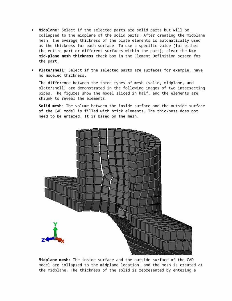
stationary frame. This is a bonded face, and the boundary layer mesh is ideal for creating these uniform elements. For more information, see Rotating Frames of Reference.

If the Tetrahedra and wedges (boundary layer) radio button is selected in the General tab, the Tetrahedra tab will be available. The boundary layer mesh can be controlled using the Boundary layer options section. The size of the elements in the boundary layers will be controlled by the Extrusion distance based on drop-down box. If the Fraction of mesh size option is selected, the value in the Total extrusion distance field will be multiplied by the surface mesh size. If the Absolute length dimension option is selected, the value in the Total extrusion distance field will be used If the Percentage average local size option is selected, the value in the Total extrusion distance field will be used as a percentage of the mesh size in the area of the boundary layer. You can control how the mesh size increases in adjacent boundary layers using the Growth rate field. The value in this field will be the ratio of the average edge length of elements in adjacent layers. This value must be greater than 1. You must specify how many boundary layers you want to be generated in the Layers drop-down box. TipBoundary Layer mesh should be thinner than element size; otherwise, meshing problems can occur.

When using the LES turbulence model (see Turbulence Options), the mesh size at the wall needs to be thin enough to capture the boundary layer effects. When using the k-epsilon turbulence model, the boundary layer mesh does not need at be as thin. However, the thickness needs to be within a certain range to give accurate results. The near wall elements should be thick enough to fully contain both the viscous sub-layer and the transition layer. This condition is best satisfied when the Y+ value is around 30. (Ranges of Y+ between 5 and 300 may be acceptable; at least a few elements/nodes should be inside the boundary layer Y+ < 300). If the results are outside of this range after the analysis is completed, the mesh should be adjusted accordingly. (See the page Results: Results Environment: Results Menu: Fluid Flow Results Menu.) TipWhen using the k-epsilon turbulence model, use just one layer in the boundary layer mesh. This results in better convergence than if multiple layers are used. Multiple layers can be used as long as the other boundary layer elements are outside of the fluid boundary layer.

Use advanced meshing options

Activating the Provide detailed status information check box in the Advanced tab will output detailed meshing information to a log file. This information may be useful in determining why a mesh has failed.

During the solid meshing process, errors may be found in the surface mesh. If the Fix errors and continue solid meshing option is selected in the Connectivity voids check drop-down box on the Advanced tab, the mesher will attempt to correct the surface mesh. If the Do not fix errors option is selected, the mesher will stop. The surface mesh must be corrected before the solid mesh will be created.

If the Disable self-intersection check box on the Advanced tab is activated, the solid mesh process will not check to determine if the surface mesh intersects itself. This check box should only be activated after an original solid mesh has been generated on the model.

If the Attempt completion with errors check box on the Advanced tab is activated, a solid mesh will be generated regardless of errors in the surface mesh. This may result in

voids throughout the model. If this check box is activated, you should be sure to verify the solid mesh.

Mesh a gasket

Any part destined to be defined as gasket elements needs to have a mesh with only one element through the thickness. This is accomplished in a CAD solid model by assigning the part to a Gasket solid mesh with one of these methods:

Set the element type for the part to 3D Gasket.

Right-click the part in the display area or the tree view and select the CAD Mesh Options Part command. Then with the Mesh type set to Solid, click the Options button, choose the Solid button, and set the solid mesh type to Gasket.

Nonpositive Jacobian Errors or Distorted Elements

Topics in this section Effects of Microholes within a Solid Mesh Nonpositive Jacobian Errors or Distorted Elements

Effects of Microholes within a Solid Mesh

Abstract

The accuracy of finite element analysis (FEA) of solid models generally benefits from meshes composed of elements of high geometric quality. Autodesk Simulation has developed an automated solid meshing method that enforces strict geometry checks used by NASTRAN processors. This automatic generation of solid elements can result in meshes with small internal voids. Generally, such voids will only occur when considering parts with complex shapes, including CAD solid models. In this paper, we consider results obtained with meshes that contain such voids. The automatic meshing method is optimized to minimize the size of these voids, thus the term microholes. These results are compared with others obtained using fully filled parts, as well as with analytical solutions. We demonstrate how models with microholes and those with fully filled meshes both result in insignificantly different results.

Introduction

The application of FEA to 3D solid models requires the generation of meshes composed solely of tetrahedral elements or of a hybrid combination of bricks, wedges, pyramids and tetrahedra. The latter approach is preferred when considering solids whose surface is represented using quadrilaterals, and can be further refined to avoid the generation of pyramids. Proper mesh generation attempts to build the best quality elements for codes like NASTRAN. In general, automatic mesh generators aim to produce elements with low aspect ratios. Autodesk Simulation’s automatic solid mesh generators not only minimize aspect ratio, but build elements adhering to the geometry checks utilized by NASTRAN processors.

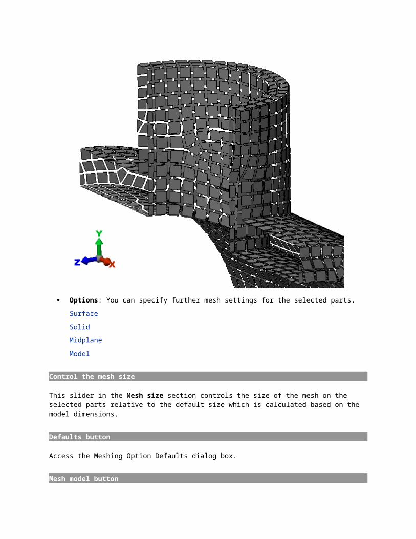
These geometric checks include: aspect ratio, collapse ratio, taper ratio, interior angle, skew angle, twist angle, and warp factor.

It is desirable to completely fill a solid with a mesh composed solely of elements adhering to high-quality criteria, such as those discussed above. One would expect that such a mesh would produce highly accurate FEA results. The problem is that obtaining such a mesh is not always possible for models with complex geometry. This is primarily because detailed geometric features constrain the mesh generator so as to prevent the creation of meshes with gradual transitions between small and large element sizes. The advent of CAD has made models with detailed features commonplace. If you utilize a mesh size comparable or smaller than the feature size, then transitions are not needed, and the high-quality constraints can be enforced throughout fully filled parts. Nevertheless, this approach requires extremely small mesh sizes, which produces models with an unpractical number of elements, whose solution requires unreasonable computing resources. After all, the goal of the engineer is usually to maximize accuracy, while maintaining a practical approach.

In an attempt to avoid the impractical requirement of extremely fine meshes to satisfy both the filled solid and high element quality constraints, we have developed an automatic meshing method that leaves insignificantly sized voids - within the solid. The primary goal of this scheme is to provide the highest accuracy possible by building only elements adhering to strict geometric quality. We have developed another automatic meshing method that completely fills the parts by first applying the high-quality meshing method that results in microholes, and then fills the small voids with elements that may not necessarily adhere to the geometry checks. As we will show, neither the meshes with microholes, nor the full meshes with a few elements violating the geometry checks, result in significant accuracy losses. After all, the latter type of mesh can certainly be viewed as an improvement over common automatically generated FEA meshes. Such meshes can have numerous poor quality elements, occupying large portions of the overall volume.

Both meshing methods discussed above address this concern by building elements using a marching algorithm from the surface inward. This approach usually produces elements adhering to the strict geometry checks near the surface, and only produces microholes or lower-quality elements deep within the parts. It is desirable for the sake of accuracy to have the best quality elements near the surface, where usually the greatest gradients in FEA solutions usually occur. This is because in most FEA applications, including stress analysis, the loads and constraints as well as part-to-part interactions generally occur on the surface.

In this paper, we show how the existence of microholes can produce noticeably more accurate FEA results over comparable models with fully filled meshes. Results were obtained for analysis types based on Lagrangian formulations, which include stress, thermal and electrostatics. Models with microholes are not appropriate for Eulerian formulations, such as fluid flow analysis.

Comparison Study

The effect of microholes on an FEA solution is examined by comparing results of models with and without microholes. Specifically, we compare results of identical surface meshes whose solid meshes were obtained using the two different meshing methods. To focus on the effect of microholes, and not on mesh type, we consider only meshes using Autodesk Simulation’s hybrid solid mesh types. In either the tetrahedral or the hybrid solid mesh types, microholes occur when tetrahedral elements cannot be built to fill a given small void. In both meshing methods the tetrahedral elements are generated only in the final meshing stages. The models considered in this study may at first appear to have relatively simple geometry,

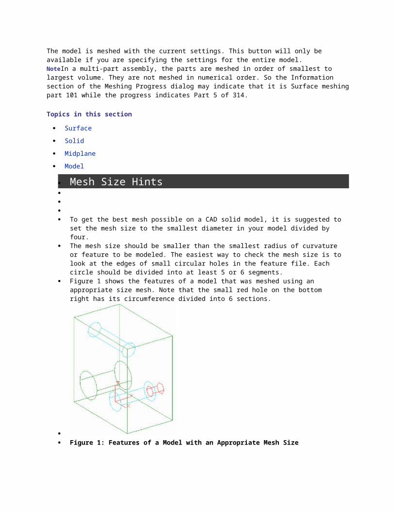
lacking the small features known to be the cause of microholes. Nevertheless, because localized mesh refinement was utilized, the resulting abrupt transitions in the surface mesh size prompted the production of microholes. It should be noted that all of the models presented in this paper contain typical to large microhole volume fractions, thus maximizing their effect.

Figure 1 depicts the surface geometry of a three-part CAD assembly. This surface mesh resulted in a relatively large 0.00207 microhole volume fraction. Static Stress with Linear Material Models and Natural Frequency (Modal) analyses were conducted on this model, and on its fully filled counterpart. Figure 2 shows how similar stress results are obtained for both versions of the model. The modal analysis was utilized to obtain the first five natural frequencies, and, as Table 1 shows, both versions of the model again gave solutions with insignificant engineering differences.

Figure 1: FEA model, including mesh, of a three-part assembly of a circular rod bonded to two brackets, which are fixed using boundary conditions on the edges of the holes located on their flat ends (red triangles on the underside). In the Static Stress with Linear Material Models analysis, a surface force of 5.0 x 108 dynes is applied on one end of the rod (yellow arrows).

Figure 2: von Mises stress distributions obtained from the Static Stress with Linear Material Models analysis of a three-part assembly of a circular rod bonded to two brackets. The figure on the left is for the model without microholes, whereas that on the right is for the model with microholes. The latter predicts a maximum stress 0.31% greater than the former.

Mode number, n

Models without Microholes

Models with Microholes

Percent difference (%)

1 1132.8 Hz 1129.2 Hz 0.318

2 1169.9 Hz 1168.1 Hz 0.154

3 1228.1 Hz 1226.1 Hz 0.163

4 2877.4 Hz 2875.0 Hz 0.083

5 3007.0 Hz 3003.2 Hz 0.126

Table 1: Modal frequencies obtained from Natural Frequency (Modal) analysis of a three-part assembly of a circular rod bonded to two brackets. Note how all these frequencies compare to within 0.32%.

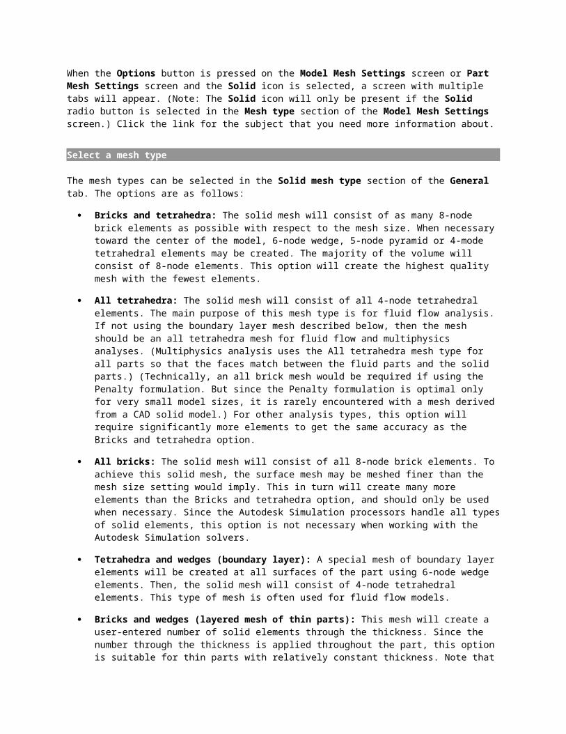
Figure 3 depicts the Steady-State Heat Transfer results of a single-part model of a ring with and without microholes. The microholes resulted in a more typical 0.00046 volume fraction. As in the Static Stress with Linear Material Models analysis, both versions of the model produced highly similar results. Figure 4 depicts displacement results obtained using Autodesk Simulation’s Mechanical Event Simulation (MES) software for the two versions of the ring model. Even for nonlinear FEA, the presence of microholes did not significantly affect the results. Finally, Figure 5 depicts voltage results obtained using Autodesk Simulation’s Electrostatic Current and Voltage analysis for the two versions of the model. As expected because of the underlying similarities between electrostatic and thermal analysis, the presence of microholes had little effect on the results.

Figure 3: Temperature distributions obtained from a Steady-State Heat Transfer analysis for ring model with the base maintained at 100 °F, and a heat flux of 0.642 BTU / (sec . in2) applied to the inner surface. The figure on the left is for the model without microholes, whereas that on the right is for the model with microholes. The latter predicts a maximum temperature 0.349 °F greater than the former.

Figure 4: Displacement magnitude distributions obtained from a Mechanical Event Simulation (MES) analysis for a ring model with the outer surface fixed and a time-

proportional pressure reaching a maximum of 100 lb/in2 seconds applied on the inner surface. The results are at the end of a 0.1 second event. The figure on the left is for the model without microholes, whereas that on the right is for the model with microholes. The latter predicts a maximum nodal displacement 0.56% greater than the former.

Figure 5: Voltage distributions obtained from Electrostatic Current and Voltage analysis for ring model with a voltage of 100 V applied on the inner edge of top surface, and 0 V applied on the outer edge of the outer surface. The figure on the left is for the model without microholes, whereas that on the right is for the model with microholes. A comparison of the maximum voltage on the outer top edge shows a difference of 0.02% between the two models.

Conclusions

A new automatic meshing method with emphasis on accuracy has been developed. This method only generates elements of high geometric quality, yet leaves microholes. This meshing method has been extended to fill these small voids with elements that may not satisfy high geometric quality constraints. Both methods generate meshes capable of producing highly accurate FEA results. Several examples demonstrated how FEA models with typical to large volume fractions of microholes and those with fully filled meshes produced results of equal engineering accuracy.

Nonpositive Jacobian Errors or Distorted Elements

Solution problems can occur when very long, skinny tetrahedral elements are created by the solid mesher. For linear stress analysis, these elements have near zero or negative volume (due to round off) that cause solution difficulty such as Jacobian is negative or poor precision results (in the Results environment, use Results Contours Voltage and Current Current Flux Precision.)

With nonlinear stress analysis, distorted elements can give warning messages such as ** Warning: distorted element 2456 in part 2: maintaining its integrity.

Take a look at the Solid Mesh Statistics shown below. (From the FEA Editor environment, go to Mesh Mesh View Mesh Results and look at the Part information. For the last solid mesh generated, the solid mesh statistics are also in the .XLG file.) After the general recap, columns of numbers are given for each of the statistic lines. From left to right, these represent the Tetrahedral (4-node) elements, Pyramid (5-node), Wedge (6-node), and Brick (8-node) elements. The Jacobian problem occurs when the Max. length ratio is relatively large. This usually occurs for the 4-node elements.

Mesh type Mix of bricks, wedges, pyramids and tetrahedra

Watertight Yes

Mesh has microholes No

Total nodes 966

Volume 136.799506 in^3

Total elements 1511

Tetrahedra Pyramids Wedges Bricks

Elements 744 384 140 243

Volume % 10.96 12.33 9.31 67.38

Max. length ratio 105.2 44.6 5.4 2.3

Avg. length ratio 5.9 4.1 3 1.5

Avg. aspect ratio 1.3 1.4 1.2 1

Unconstrained aspect ratio 3.1 3.2 1.3 1.1

In the example above, 243 brick elements were built, 140 wedge elements, 384 pyramid elements, and 744 tetrahedral elements were created. For the maximum length ratio, the brick elements were 2.3, and the tetrahedral elements were 105.2.

In general, there is no guide line for what the maximum acceptable length ratio can be. Each model is different, so a value of 10000 may be acceptable in some cases, where as some models may have problems with much lower numbers.

There are a couple of options to reduce the problem of the length ratio. If the part was not meshed with the mircrohole option activated, consider using it. This will remove the sliver elements with large length ratios. (See the page The Effects of Microholes within a Solid Mesh for a discussion.) In the FEA Editor environment, select the part or parts to re-mesh, right-click, and choose Created Solid Mesh Options Allow microholes. Then create the solid mesh and run the analysis with the better mesh. (The solid mesh dialog can also be accessed from Mesh Mesh Create Solid Mesh. Parts to be meshed need to be selected first.)

The next option is to re-create the solid mesh with the maximum aspect ratio set. The goal is to reduce the value until the solid mesh either fails to create a complete mesh or the solid mesh engine does not reach the ratio you specified. So, you could run the solid mesh engine and cut the aspect ratio in half (50, 25, and so on), until you reach the limit. In the FEA Editor environment, select the part or parts to re-mesh, right-click, and chooseCAD Mesh Options Create Solid Mesh Quality. (See Controlling the Aspect Ratio on the page Solid for a description of the input.) Then create the solid mesh and run the analysis with the better mesh.

Be sure to check the log file after each solid mesh generation. If the solid mesh engine was unable to completely fill the volume with the parameters you specified, there will be an error message. The following is a partial listing of a log file.

TYPE OF OPERATION: Meshing only surface defined by part 4 Generating bricks, wedges, pyramids and tetrahedra elements Keeping maximum aspect ratio below 10.0 ERROR NUMBER 300: Cannot continue meshing solid; yet, solid is unfilled. FINAL STATISTICS: Still have: 4 nodes; 6 lines; 4 triangles Elements built (4,5,6,8 noded): 1953 (1153, 482, 73, 245 )

Finally, if the model is not located near the origin, then round-off errors in the nodal coordinates can create distorted elements. If the model is located entirely with coordinates in the thousands, then another solution would be to move the CAD model closer to the origin. (Ideally, the model should be centered at the origin.) This requires that the entire model be imported and re-meshed.

If the Jacobian problem still occurs, then the surface mesh must be changed to get a different solid mesh.

Midplane

When the Options button is pressed on the Model Mesh Settings screen and the Midplane icon is selected, a screen with one tab will appear. The Midplane icon will only be present if the Midplane radio button is selected in the Mesh type section of the Model Mesh Settings screen.

Thickness control section

User-specified maximum thickness: By default, the midplane mesh process will search each area of the part and create the midplane mesh along the smallest thickness that

it detects. To specify a value to be used, activate this check box and enter the thickness in this field. Any area of the model that has a thickness larger than this value will not be midplane meshed.

Maximum allowed thickness variation: If this check box is activated, the midplane mesh process will only convert the mesh on a part to a midplane if the difference between the maximum thickness and the minimum thickness in the part is less than the value specified in this field.

For complex geometric configurations that include junctions and intersections, a more accurate midplane mesh may be achieved by activating the Use junction method check box. If this check box is activated, a chordal axis transform (CAT) algorithm will be used to generate the midplane mesh. This method may eliminate discontinuities at the junctions and may provide a better approximation of the midplane of the geometry.

Model

Activating the command: Mesh Mesh 3D Mesh Settings Options Model button

When the Options button is pressed on the Model Mesh Settings screen and the Model icon is selected, a dialog with two tabs, the General and Advanced tabs, will appear. The Model icon will be present regardless of which radio button is selected in the Mesh type section of the Model Mesh Settings dialog.

Which options appear on the Model General tab depend on whether the option Mesh Mesh Use VCAD is activated or not. Each control described below will be identified as working with the VCAD mesher, with the legacy mesher, or both. NoteVCAD refers to Virtual CAD which is a representation of the CAD model in memory. When Mesh Mesh Use VCAD is activated, the virtual CAD mesh engine is used. When not activated, the pre-version 21 meshing routine is used. Because of the benefits of the virtual CAD mesh engine over the legacy mesh engine, the legacy mesh engine is recommended only if there is a problem with the virtual CAD mesh engine on a particular model.

General tab Default Meshing options section:

Automatically refine surface mesh: (Available only when using the legacy mesh engine.) If this check box on the General tab is activated when the model is meshed, a surface mesh will be created on the model. After the surface mesh is created, refinement points will be added depending on the geometry. The model will be meshed again with the refinement points active. If the Solid radio button is selected in the Mesh type section of the Model Mesh Settings screen, a solid mesh will then be generated.

Use automatic geometry-based mesh size function: (Available only when using the VCAD mesh engine.) This one control governs multiple aspects of the surface mesh that normally would require you to set up multiple inputs. In general, it automatically refines the

mesh in the areas of curves surfaces. The particular effects are summarized in the following table.

Activated Not Activated

When the mesh size is set based on Percent of automatic (i.e., using the slider), a different mesh size is used for each part. The mesh size is based on the size of the individual part, the number of curves, bounding box dimensions of the part, average length of curves, and so on.

The mesh size is the same in each part, and is based on the size of the entire model.

Curved surfaces are meshed more finely depending on the curvature of the surface. A limit is used on the deviation between the planar element and the curved surface, and so on.

Curved surfaces are meshed based on the user-entered mesh size and refinements.

The mesh size is anisotropic on curved surfaces, meaning that the ratio of the element's length divided by the element's width is not forced to be near 1. For example, take a mesh size of 1-inch. The mesh in a fillet of 0.5-inch radius and 20-inches long may have elements roughly 0.25-inch by 1-inch.

The mesh size is isotropic. The element's length divided by the width is near 1.

The refinement settings on the Options tab of the Model Mesh Settings Surface dialog are disabled. You cannot set the values.

The refinement settings on are available to change.

In general, the default mesh size is larger. In general, the default mesh size is smaller.

Perform solid meshing at time of analysis: (Available when using either mesh engine.) If this check box is activated and the Solid radio button is selected in the Mesh type section of the Model Mesh Settings screen, the model will not be solid meshed until the analysis is performed. This is convenient for large models that may take a significant amount of time for a solid mesh to be generated. With this option, this time will be combined with the analysis time instead of in a separate operation. If this check box is not activated, a model will be solid meshed immediately after the surface mesh is created.

Use virtual imprinting: (Available only when using the VCAD mesh engine.) When activated, the faces of different CAD parts will be split in memory where they intersect each other, without creating additional surface numbers (that is, a virtual imprinting of one surface on another). Since the matching virtual surfaces are meshed only once, this will result in a better quality mesh. When unchecked, mesh matching is accomplished by meshing both surfaces of the parts and adjusting the mesh on one part to conform to the mesh on the other part. See Figure 1. TipTo take full advantage of smart bonding (see paragraph Do not match the mesh of contact pairs when applicable below), deactivate Use virtual imprinting. This helps the mesh to not match. However, if other parts of the model use surface contact, then activating Use virtual imprinting is beneficial.

(a) Example solid model consisting of an assembly of multiple parts.

(b) Use virtual imprinting not activated. Surfaces are not created at the arrows.

(c) Use virtual imprinting activated. The surface of the pole is split where the gussets make contact (arrowed), making a new surface in the virtual copy of the model. (New surfaces are not created in the real model.)

Figure 1: Use virtual imprinting in a Solid Model

Since virtual imprinting operates where adjacent parts are in contact, the Use virtual imprinting option is not shown and would have no effect when working on single-part models.

Perform imprinting within parts: (Available only when using the VCAD mesh engine.) The Use virtual imprinting option (described above) acts on part-to-part matching; the Perform imprinting within parts does a similar matching between surfaces and feature lines within a part. This is most useful with plate/shell models where the entire model may come in as a single part. Without using the imprinting within a part, it is possible that the mesh on one surface will not match the mesh on an adjacent surface. See Figure 2.

(a) Example plate model consisting of one part.

(b) Perform imprinting within parts not activated. The line contact is not created at the arrows. The mesh of the gusset may not match the mesh of the pole.

(c) Perform imprinting within parts activated. The surface of the pole is split where the gussets make contact (arrowed), making a new feature line in the virtual copy of the model. The meshes will match.

Figure 2: Use virtual imprinting in a Plate/Shell Model Note

Note that surface knitting of the model is a similar but separate function to imprinting that creates additional surfaces in the model. Whereas surface knitting only works on a part-to-part basis wherever surface areas are in common, imprinting will work on a part-to-part basis and within a single part, and it can create area, line, and point intersections. See the page Opening Models: Surface Knitting for details on surface knitting.

Both Use virtual imprinting and Perform imprinting within parts detect where feature lines of one surface lie on the surface of an adjacent part or surface. It does not create an intersection if the two surfaces are passing through each other (such as an interference).

Mesh matching section:

CAD models are not perfect. Even if the parts are drawn in perfect contact, the internal representation of the surfaces may result in the matching surfaces that are not coincident. In other situations, parts are drawn in their as machined or stress-free condition even though the assembled parts may cause the dimensions to change. For example, the parts in a press-fit assembly are drawn with an interference. Mesh matching tolerances are used to compensate for such discrepancies. Any two nodes that are within the mesh matching tolerance will be snapped together.

On-surface tolerance based on: (Available when using either mesh engine.)

Fraction of surface mesh size: If this option is selected, the surface mesh process will search for nodes within the radius defined by the average length of the elements (in the surrounding area) multiplied by the value in the Tolerance value field. Nodes

within this radius will be snapped together. Thus, this option results in a different matching tolerance at each region of the model if the mesh size varies.

Absolute length dimension: If this option is selected, the surface mesh process will search for nodes within the radius specified in the Tolerance value field of each node to match the meshes of coincident surfaces.

Fraction of automatic mesh size: This option is similar to Fraction of mesh size in that the nodes are snapped if they are within a distance of the mesh size multiplied by the value in the Tolerance value field. The difference is that the mesh size is not based on the size of the elements at the area in question. Instead, the mesh size is based on the size of mesh that would result if meshed at 100% mesh size. Thus, setting a different mesh size and using refinement does not affect the tolerance dimension. However, the 100% mesh size is affected by which parts are selected for meshing.

Tolerance value: The value in this field will determine how far the surface mesh process searches for node on coincident surfaces to match the meshes. The meaning of this value --- whether it is a dimension with units of length or a multiplier --- will depend on the option selected in the On-surface tolerance based on drop-down box.

Do not match the mesh of contact pairs when applicable: (Available only when using the VCAD mesh engine.) This option is used to not force the mesh to match or align on two touching surfaces. Since the mesh will not match, the parts will not be connected together. (Note that the mesh may still be the same size and therefore matched if the surface areas are identical.) This option is used only in these situations:

When the analysis is set to use smart bonding (see the page Meshing Overview: Creating Contact Pairs: Types of Contact)

Mechanical Event Simulation (MES) and nonlinear stress when surface to surface contact is defined between the two surfaces. (The analysis will run faster by not matching the mesh between two contacting surfaces.)

In other analysis types, setting the contact type to Free will accomplish the same goal since the parts will be able to separate. Note

For the Do not match the mesh of contact pairs when applicable to work, define the applicable contact type before meshing the model. If the applicable contact type is defined after the model is meshed, the model should be remeshed to not force the match of the nodes.

There are some points where the mesh has to align. Imagine two cubes of the same size in contact. Since the four corners are at the same location, these nodes will match. The rest of the mesh will not be forced to match. Although the four corners match, separate nodes will be created when the model is analyzed.

In MES, do not use the Do not match the mesh of contact pairs when applicable if using Point to Point contact type in surface-to-surface contact. Point to Point requires the meshes to match.

Advanced tab

The Advanced tab includes the key tolerances used in the virtual CAD imprinting operations when merging and imprinting (or splitting) multiple entities (vertices, edges, and so on). Consequently, this tab is not shown if the Use virtual imprinting option (described above) is unchecked. In a single part CAD model, the tab is not shown if the Perform imprinting within parts option (described above) is unchecked.

If the CAD model is failing to mesh properly, and it appears to be a problem with small discrepancies between the parts, surfaces, edges or vertices, then tweaking these tolerances and re-meshing may solve the problem.

Since each operation involves two entities --- such as two vertices being merged, or imprinting an edge onto a face - two tolerances are used with each operation. The two entities are considered to be within the operating distance of each other if the distance between the entities is less than the sum of the two tolerances. For example, two vertices are merged if the distance between them is less than the Merge vertex tolerance for the first vertex plus the Merge vertex tolerance for the second vertex.

The operations performed between two entities are as follows: Operation Tolerance 1 Tolerance 2 Figure

Merging two vertices

Merge vertex tolerance for the first vertex

Merge vertex tolerance for the second vertex

Merging two edges

Merge edge tolerance for the first edge

Merge edge tolerance for the second edge

Imprinting a vertex onto an edge

Imprinting vertex tolerance

Imprinting edge tolerance

Imprinting an edge onto another edge

Imprinting edge tolerance for the first edge

Imprinting edge tolerance for the second edge

Imprinting an edge onto a face (normal to the face)


Imprinting face tolerance (normal)

Imprinting an edge onto a face (lateral to the face)


Imprinting face tolerance (lateral)

The tolerance multipliers used in the above operations are either entered as an explicit value in the Multiplier field, or with the slider to adjust the value between the recommended minimum and maximum value. The tolerances are as follows:

Tolerance Description

Merge vertex tolerance

Controls the tolerance used in merging vertices that may belong to either the same or different parts. The smallest length of all edges incident on a vertex is multiplied by the tolerance value to determine the tolerance (in units of length) at the vertex.

Merge edge tolerance

Controls the tolerance used in merging edges that may belong to either the same or different parts. The edge length is multiplied by the tolerance value to determine the tolerance (in units of length) used.

Imprinting vertex tolerance

Controls the tolerance used in imprinting vertices on adjacent edges. The smallest length of all edges incident on the vertex is multiplied by the tolerance value to determine the tolerance (in units of length) used.


Controls the tolerance used in imprinting edges with vertices, other edges, or faces. The edge length is multiplied by the tolerance value to determine the tolerance (in units of length) used.

Imprinting face tolerance (normal)

Controls the tolerance used in imprinting a face with another edge. Diagonal lines are created across the bounding box that surrounds the face. The maximum diagonal length is multiplied by tolerance value to determine the tolerance (in units of length) used. Note that this tolerance is used in the direction normal to the face.

Imprinting face tolerance (lateral)

Controls the tolerance used in imprinting a face with another edge. Diagonal lines are created across the bounding box that surrounds the face. The maximum diagonal length is multiplied by tolerance value to determine the tolerance (in units of length) used. Note that this tolerance is used in lateral or tangential direction of the face and can be used to avoid narrow regions.

Mesh Results

After a mesh has been successfully generated for your model, you will be prompted to review the results. Press the Yes button. If you are not prompted or want to review the mesh results at a later time, use Mesh Mesh View Mesh Results. The Meshing Results dialog box appears.

If the Model button is pressed, the number of parts in the model that were meshed with each mesh type will be listed with the number of elements generated. If the Part button is pressed, you will be able to toggle through the mesh results for each part in the model.

If a mesh attempt is unsuccessful, the Problems button will become available. When the Problems button is pressed, the Problem Summary is displayed, showing all errors and/or warnings logged by the mesh engine. In the “Problem Summary,” errors are listed first, followed by warnings. Beneath each error/warning you will find a list of offending parts/surfaces. Each of the parts/surfaces listed is a link to click. NoteSurfaces indicated by gray text and an asterisk lack CAD surface data, likely due to a bad CAD model or bad import operation. Autodesk Simulation is unable to render the indicated surfaces causing the mesh engine to fail.

When a link for a part is selected the following actions are performed:

All other parts are hidden

The selected part is enclosed (View Navigate Enclose)

The display is set to “Shaded with Mesh” (View Appearance Visual Style Shaded with Mesh)

Color is viewed by layer (View Appearance Color By Layer)

Only layers 2 and 3 are shown (Draw Design Layer Control )

TipSwitch between View Appearance Visual Style Shaded with Mesh and View Appearance Visual Style Mesh to get a context for the location of the layer 2 and 3 mesh lines.

When a link for a part is selected in the Warnings section, the following actions are performed:

All other parts are hidden

The selected part is enclosed (View Navigate Enclose)

The display is set to “Edges" (View Appearance Visual Style Edges)

Color is viewed by surface (View Appearance Color By Surface)

The unmatched edges are shown by orange colored lines, and multi-matched edges are shown by blue colored lines (View Appearance Only Bad CAD Features)

TipSwitch between View Appearance Visual Style Edges and View Appearance Visual Style Shaded with Edges to get a context for the location of the unmatched or multi-matched edges. Also see Feature Matching.

When a link for a surface is selected, the following actions are performed:

All other parts, except the one containing the selected surface, are hidden

The surface is selected

The display is set to “Shaded with Mesh” (View Appearance Visual Style Shaded with Mesh)

Color is viewed by edge (View Appearance Color By Edge)

The zoom level is set to capture all offending surfaces

The goal behind the view changes is to aid you in finding the problematic geometry so that it can be fixed.

When the “Meshing Results” dialogue is dismissed, all shading, views and visibility revert back to what they were previous to clicking any of the part/surface links. Tip

If you click links in the Problem Summary, your model view and visibility could change. To ensure your model resets to the view settings in effect prior to opening Meshing Results, select Restore view and visibility changes on exit prior to closing the dialog box.

Select Keep current view when clicking on link to maintain the current model orientation with each surface click.

Watertight Problems in Meshes When generating a solid mesh on a part using Create Solid Mesh (or during the Verifying surface mesh stage of creating the surface mesh on a CAD solid model), the solid mesh engine first checks if the part is watertight. Watertight means that the mesh on all of the surfaces is complete, the lines of the mesh create valid elements, and the mesh properly connects to adjacent surfaces around the perimeter so that the volume is fully enclosed. (If you imagine puncturing the part with a hypodermic needle and trying to fill it with water, the model is watertight if it would not leak. When elements are missing or not properly connected together at edges, then the water would leak, and the mesh is not watertight.) Figure 1 shows an example of a watertight problem.

Figure 1: Model with Watertight Problem. Half of the surface of the cylindrical hole is missing from the CAD model. (The outside face of the cube has been hidden to show the inside.)

Follow this procedure for locating the cause of the watertight mesh problems.

1. After the part or model has been meshed, a dialog will indicate that some parts failed to solid mesh and/or had watertight problems. After closing the mesh dialogs, the tree view will flag the parts with problems using a yellow exclamation point (!). (Or, use Mesh Mesh View Mesh Results to review which parts had problems. The Problems button will summarize the problem parts, and Log File under the Part button will give details about the reason the appropriate part failed.)

2. Use the Draw Design Layer Control command. The elements in the vicinity of the watertight problems are on layers 2 or 6. Hide the other layers (and optionally the other parts that meshed) and zoom in on the problem. By displaying the complete mesh and just the problem layers, it should be possible to understand the cause of the watertight problem. For example, does layer 2 or 6 outline a hole in the mesh? Are the elements severely distorted or twisted?

3. Some of the options to fix the problem are as follows:

For CAD Solid Models. If the problem is a missing surface or holes in the mesh, check the original CAD model for possible problems. In some cases, extremely small or thin surfaces (such as a zero radius fillet) may result in a mesh that does not match between adjacent surfaces. After adjusting the CAD model, try the mesh again.

For CAD Solid Models. If an entire surface is missing or jumbled, check the tolerances in the FEA Editor environment. Start with the Mesh Mesh Feature Matching command. Check if the problematic part contains any unmatched or multi-matched features. If so, change the Feature matching mesh size and click

the Apply button. The goal is to eliminate the unmatched and multi-matched edges by changing the tolerance. (See also Feature Matching.) If the part or surfaces in the problem area are not shaded correctly, use View Appearance CAD Rendering and change the rendering settings. The goal is to get the settings that renders the model accurately.

For CAD Solid Models. Try a finer surface mesh either in the entire model (Mesh Mesh 3D Mesh Settings), in just the part that failed (right-click part, then CAD Mesh Options Part), or by using refinement points in the problem area (select a vertex or multiple vertices in the problem area, then right-click and choose Add Refinement Points). After changing the mesh size, try to create the mesh again (Mesh Mesh Generate 3D Mesh ).

For CAD Solid Models and Hand-built Models. If the problem area is small, it may be possible to manually fix the mesh in the FEA Editor environment. Add lines and/or delete lines as necessary to create valid elements. This could be done line-by-line, or by copying or extruding surfaces, and so on. In some cases, the global snap (Draw Modify Global Snap) is beneficial to snap a repair mesh to the existing mesh. Keep in mind that valid surface elements are composed of 3 or 4 sided regions. If adding lines, be sure to use the appropriate part, surface, and layer number for the new lines. After repairing the mesh, right-click the part and choose CAD Mesh Options Create Solid Mesh to create the mesh and check if the problem is fixed.

Joint components

In many models, it is necessary to simulate joints and pinned connections for rotational purposes. Modeling the actual joint components with surface to surface contact will create very long run times. In most cases, the effects on the actual joint components are not important. The easiest way to simulate a joint or pin without a long runtime is to create a Truss element along the axis of the joint and connect it on the ends to the part that will rotate about the axis. Since truss elements cannot resist rotation, this creates an effective pin joint. Adding these lines to an existing meshed model can become quite tedious. The Create Joint command provides a quick alternative to this process when working with a CAD model. Using the Create Joint you can select the surfaces that you want to use to create the joint. When you create the surface mesh, truss elements will be constructed between these surfaces.

Figure 1: Schematic of a Pin Joint Instead of modeling a true pin, a clevis and eye are connected with a pin-style joint. Truss elements from two points (A and B) are connected to each node on the selected surfaces. (To simplify this figure, only one line is shown from each point to each surface. Also, points A and B are moved outside of the parts for clarity.) A pin joint can be visualized as sets of space trusses. The truss elements (blue lines) that extend from the surfaces of the clevis (green body) to point A form one space truss. If the truss elements are sufficiently stiff, point A cannot move relative to the surface of the clevis. Likewise, a second space truss is formed from the clevis to point B. Likewise, space trusses are created from the eye (light blue body) to points A and B. Because truss elements have pinned connections, the space trusses and bodies they connect to can rotate about the line A-B, but they cannot translate independent of each other. Thus, a pin is simulated.

To create a joint, follow the steps below. NoteIf the joint will be attached to a part that includes the midside nodes, it is suggested that you activate the midside nodes before generating the joint. This way, the joint will be attached to the midside nodes, too. If the midside nodes are included after generating the joint, then the joint will only be connected to the corner nodes.

1. Optionally select all of the surfaces that you want to be involved in the joint. You can either click the surfaces on the model (be sure to hold down the <Ctrl> key to select multiple surfaces) or select the heading for those surfaces in the tree view (again be sure to hold down the <Ctrl> key to select multiple surfaces). You must have the Selection Shape Point and Selection Select Surfaces commands active to select surfaces by clicking them in the model.

2. Select Mesh CAD Additions Joint or press the button.

3. The Create Joint dialog will appear to allow you to enter the specifications for this joint. The surfaces that you selected before entering the Create Joint screen will be listed in the Participating surfaces section. If surfaces were not selected before, or

if additional surfaces need to be added for the joint, select the surface or surfaces and click the Add button.

4. Select the type of joint that you want to create in the Joint drop-down box.

Pin joint (lines to axis endpoints): This option will create a classic pin joint where the nodes at each end of the surfaces included in the joint are connected to the opposite end of the joint axis. This type of joint will allow the model to rotate around the axis. See Figure 1.

Universal joint (lines to axis midpoint): This option will create a classic universal joint. The nodes at either end of the model will be connected to the midpoint of the axis. This type of joint will allow the model to rotate about the axis as well as swivel about the center point of the axis. See Figure 2.

Figure 2: Schematic of a Universal Joint Compare the universal joint to the pin joint. Instead of the space trusses being connected to two points (A and B in Figure 1), the space trusses of a universal joint are connected to one point O. Because truss elements have pinned connections, the space trusses and bodies they connect to can rotate about point O, but they cannot translate independent of each other. Thus, a universal or ball-and-socket joint is simulated.

5. If you want the joint creator to decide where the axis of rotation will be, based on the geometry of the surfaces involved in the joint, select the Automatic detection of axis/center-point radio button. To specify the axis of rotation, select the Manual axis/center-point specification radio button and enter the X, Y, and Z coordinates in the appropriate field. If your joint is a pin joint, you will have to enter the coordinates for the two end points of the axis. If your joint is a universal joint, you will have to enter the coordinate for the center point.

6. Press the OK button. If the mesh already exists, the lines for the joint will be created.

To create another joint, repeat the process.

To edit the specifications of a joint, select it in the Meshes branch of the tree view, right-click, and choose Edit.

To delete a previously created joint, select it in the Meshes branch of the tree view, right-click, and choose Delete.

If the mesh does not exist when the joint is defined, then when you execute the Mesh Mesh Generate 3D Mesh command the surface mesh will be created as usual, and then the joint application program will create the lines for the joint (either truss or beam elements). These lines will be placed in the next part available in numerical order. If you defined multiple joints, each joint will be placed in a unique part.

Potential pin joint issue

When two parts are in contact (no gap between them) and the contact type is free or surface contact, the elements of the pin joint are connected to the nodes on one of the parts, not both parts, at the contact face. This connection methodology prevents the parts from becoming locked to each other, which would occur if coincident nodes from two parts were connected to the same truss element. The joint must be free to articulate. Considering the approximation being used for pin joints, this situation is usually not a problem. However, if the joint behaves as if it is locked, then change one or both CAD parts to include a gap between the joint surfaces of the parts. Specifically, use different hole diameters, or add a chamfer around the contact edge as shown in the following figure.

Parts 1 (light blue body) and 2 (green body) are in surface contact. Two sets of nodes exist along the line C-D. However, the elements of the pin joint (lines in blue) are generally connected to only one set of nodes along C-D, not to both set of nodes. So, the joint is free to articulate. If, for some reason, the joint behaves as if it

By placing a chamfer on one or both parts, the pin joint is not connected to a series of coincident nodes at the contact face. One set of truss elements is connected to the nodes along C-D, and another set of truss elements are connected to nodes along C'-D'. The possibility of any truss being connected to

is locked, use the modified geometry shown on the right to correct the problem.

coincident nodes of two parts is eliminated and the joint is free to articulate.

So, the joint is free to articulate. If, for some reason, the joint behaves as if it is locked, use the modified geometry shown on the right to correct the problem.

Bolts and other fasteners

Bolts, screws, rivets, and other types of fasteners appear in many designs. Depending on the level of detail needed in the area of the connection, these types of connections can be treated in one of the following manners. (Recall that the FEA model is usually an idealization of the real world, so details in the fastener may not be necessary.)

Ignore the fastener itself and assume the parts are bonded together in the area of the connection. The loads are transmitted between the parts through a full-strength connection. Regions of the model remote from the connection will give accurate results. The results at the fasteners should not be used (except for providing results to use in a hand calculation of the fastener).

Model the fastener as a beam or truss element along the centerline of the holes in the parts. The fastener is bonded on each end to the nodes of the hole, so slippage is assumed to not occur in the analysis. The results are reasonable in all areas of the model, given the approximation of the fastener to part interaction.

Model the fastener with brick elements. The contact between the fastener and connected parts can either be bonded (no slippage), or contact between the parts can be included. These results are the most realistic that can be obtained at the expense of a much more complex model and longer runtime.

This page describes the beam element approach. For simplicity, the type of fastener will be called a bolt although the approach can represent any type of similar fastener. For CAD models, the Generate Bolted Connection wizard automates many of the steps necessary to create and load the geometry of a fastener. To create a bolt, use Mesh CAD Additions Bolt. Three types of bolts can be created as shown in the following figures. The top row of figures shows the physical joint; the bottom row shows the FEA equivalent, where the heavy lines are beam elements created by the bolt wizard.

Bolt With Nut Bolt Without Nut The bolt is threaded (tight fit) into the bottom part (extra bolt elements connect the shank to the hole).

Grounded Bolt The bolt is threaded into the foundation or other rigid item that is not modeled. A boundary condition is placed on the end of the bolt.

Create bolts in a CAD model

The bolt wizard creates beam elements along the centerline of the hole to represent the shank of the bolt. Additional beam elements connect the head (and nut if applicable) of the bolt to the nodes around the perimeter of the hole. Here's how to create the bolt: TipIt is more efficient to define the bolts first and then mesh the model. If the model is meshed first, it may need to be re-meshed after defining the bolts.

1. Optionally, mesh the CAD solid model. Any previously defined bolts will be re-created to fit the new surface mesh. (Meshing the model will delete all of the lines associated with all of the parts associated with bolts.)

2. Defines each bolt, one at a time, using Mesh CAD Additions Bolt. Although the bolts can be defined after generating a surface mesh, it is more efficient to define the

bolts before creating the mesh. See the description below for an explanation of each input.

3. When the OK button is clicked on the Generate Bolted Connection dialog, the following steps occur automatically:

a. Determine the axis of the hole from the selected interior hole surfaces. (The centerline is determined from the average coordinate of the nodes on the perimeter of the hole; thus, a non-uniform mesh can lead to the bolt centerline being offset from the true centerline.)

b. Draw a line along the axis of the hole, starting from where it meets the bolt head contact surface and ending where it meets the opposite faces. This line will be referred to as the bolt line.

c. Divide the bolt line into segments, one segment for each part bolted together.

d. Draw lines from the head end of the bolt line to each node on the perimeter of the head end hole. (This step is done only if the model is already meshed.)

e. If the head diameter is larger than the hole diameter, determine where the ends of each head spoke will be based on the user input head diameter and number of spokes. Seed points will be created at these locations. (If the head diameter is smaller than the hole, then no head spokes or seed points will be created.)

f. Create lines from the end of the bolt line at the head end to each seed point.

g. For a bolt with a nut, and if the nut diameter is larger than the hole diameter, seed points will be created at the locations of the ends of the spokes. (If the nut diameter is smaller than the hole, then no nut spokes or seed points will be created.)

h. For a bolt with a nut, draw lines from the nut end of the bolt line to each node on the perimeter of the nut end hole. (This step is done only if the model is already meshed.)

i. For a grounded bolt, the end of the bolt line opposite from the bolt head surface will be fully constrained. (If the model is not yet meshed, the boundary condition will appear when the model is meshed.)

j. For each set of surfaces which have been specified as a tight fit, do the following:

i. Split the appropriate bolt line segment at the midpoint.

ii. Draw lines from the midpoint to each node on the surface of the hole on that part. (This step is done only if the model is already meshed.)

k. If the bolt’s assigned part number does not exist, it will be created with the element type assigned as beam.

l. The Element Definition will be filled in automatically using a round cross section with properties equal to the bolt diameter. Note that this dictates that the last bolt created will set the diameter for all bolts in the same part.

m. Apply the bolt preload to all segments of the bolt line.

4. If any bolts have head or nut spokes and the model is already meshed, then you must remesh the model to connect the surface mesh to the spokes.

The input on the Mesh CAD Additions Bolt command is as follows. Each type of bolted connection uses similar input. Unless indicated otherwise, the following input is used for each of the three types. Refer to the following table for bolt nomenclature.

View of Nut Side. The nut diameter is smaller than the bolt, so there are no nut spokes. The nut consists of the lines that connect the bolt line to the perimeter of the hole (thin blue lines).

Side View of bolt. The bolt line is the heavy black line on the centerline of the hole. The middle section is set as a tight fit, so the nodes on the surface of the hole are connected to the center of that bolt segment (thin black lines).

View of Head Side. The head diameter is larger than the bolt, so six spokes (heavy green lines) are added based on the head diameter (dashed circle). The thin green lines connect the bolt line to the perimeter of the hole.

Part Number: Specify the part number for the bolt. This must be a new part number or an existing beam element part. If more than one bolt is assigned to the same part number, the cross sectional properties of the bolt are based on the last bolt entered or modified.

Type of Bolt: Choose the type of bolt from the drop-down list. (See Figure 1.)

Bolt diameter: Enter the diameter of the bolt shank. The cross sectional properties of the beam elements will use this diameter. (The radial spokes for the bolt head, nut, and tight fit lines will also use this diameter.)

Number of spokes: This entry controls the number of spokes that represents the head or nut. These lines are created with a radius of half the head or nut diameter. This helps to distribute the load of the bolt to a larger area and prevents stress concentrations. Note that these spokes are in addition to the lines that connect the bolt line to the perimeter of the hole.

Bolt head: Contact surfaces: This box lists the surfaces that the bolt head contacts. Select the appropriate surface or surfaces (Selection Select Surfaces) and click the Add button to add them to the list.

Head diameter: Enter the diameter of the head. This controls the length of the head spokes that will be created. If the head diameter is smaller than the bolt diameter, then no head spokes will be created.

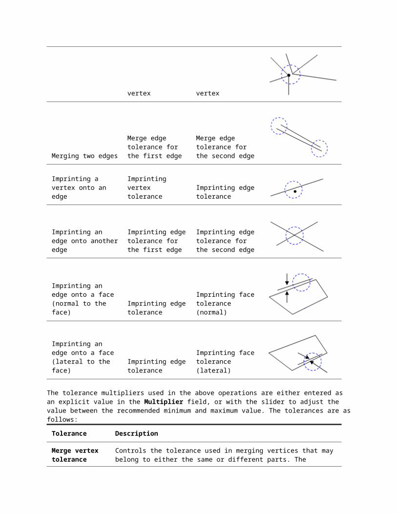
Interior hole surfaces: This box lists the surfaces of the hole. Select the appropriate surface or surfaces (Selection Select Surfaces) and click the Add button to add them to the list. (The Selection Shape Circle command is handy for this step.) Keep in mind that only one bolt can be created at a time. Each of the listed surfaces includes a Tight Fit check box. If the check box is activated, the section of bolt will be connected to each node on the surface of the hole. That is, there is no clearance between the bolt line and the hole.

Nut: Contact surfaces: For bolt types with a nut, this box lists the surfaces that the nut contacts. Select the appropriate surface or surfaces (Selection Select Surfaces) and click the Add button to add them to the list.

Nut diameter: For bolt types with a nut, enter the diameter of the nut. This controls the length of the nut spokes that will be created. If the nut diameter is smaller than the bolt diameter, then no nut spokes will be created.

Preload magnitude: To preload the joint, select either the Axial Force or Torque. If a torque is entered, it is converted to an axial force based on one of these equations when the bolt is created:

With a nut:

Without a nut:

where T is the torque magnitude, K is the friction factor, and D is the bolt diameter. For additional details on how the preload is applied to the elements, see the pages Setting up and Performing the Analysis: Linear: Loads and Constraints:Beam Preload or the equivalent page for nonlinear Beam Preloads.

Note

Preloads are only available if the bolts are analyzed as beam elements, and only in Static Stress with Linear Material Models, Mechanical Event Simulation, and Static Stress with Nonlinear Material Models.

For a real bolted connection, the bolt preload creates forces in the bolt and the members. In FEA, the beam element has an initial force but the members have 0 force. Since the structure is not infinitely stiff, one result of a preload is that the structure deforms and relieves a portion of the preload. If the bolt preload is critical in the design, it may be necessary to run the analysis with no external loads to check how much preload is lost.

Remove button: If a wrong surface is added to the bolt head, interior hole, or nut surface, select the entry in the list box. The corresponding surface is highlighted on the model. Then use the appropriate Remove button. Using standard Windows techniques, use the Shift key in conjunction with the left mouse button to select a range of surface entries in the list box, and use the Ctrl key to toggle a single selection on and off.

If multiple bolts need to be created, and especially if the bolt heads and nuts contact the same surfaces, use the Do not dismiss dialog after bolt generation option to keep the dialog open. When used, all of the input except for the Interior hole surfaces will be retained.

You can quickly specify the new interior hole surfaces for each bolt. For example, to generate three bolts connecting the same plates together, the general steps would be as follows:

1. Start the bolt wizard from Mesh CAD Additions Bolt.

2. Enter all of the input for the first bolt.

3. Activate the check box Do not dismiss dialog after bolt generation.

4. Click the OK button. The first bolt is created and the interior hole surface input is cleared. All other input is retained.

5. Add the surfaces for the interior hole surfaces of the second hole.

6. Activate the check box Do not dismiss dialog after bolt generation.

7. Click the OK button. The second bolt is created and the interior hole surface input is cleared.

8. Add the surfaces for the interior hole surfaces of the third hole.

9. Click the OK button. The third bolt is created and the dialog is closed.

10. Mesh the model if needed.

Modifying Bolts in a CAD Model

Previously defined bolts can be modified or deleted by selecting the bolt in the Meshes branch of the tree view, clicking the right mouse button, and choosing the desired command.

You can also modify the lines generated by the bolt wizard using any of the standard mesh construction techniques, such as adding lines, point move, dividing lines, intersecting, and so on. This method is not recommended because re-meshing the model will recreate the bolts, so manual modifications may be overwritten, or overlapping elements may occur.

Refinement Points

There are many situations where you are more concerned with the accuracy in certain areas of a model than others. Therefore, you will want to have a fine mesh in those areas to

ensure accurate results. However, if you create the surface mesh of the entire model with a fine mesh size, you may spend unneeded time analyzing the fine mesh in regions where the results are not as important to you.

The solution to this problem is to use refinement points. A refinement point specifies a volume of space in which a finer mesh will be generated. These can be added in the FEA Editor environment using these methods.

Refinement points are used for CAD solid models, surface mesh enhancement, and 2D mesh generation. Unless indicated otherwise, the following applies to all three types of meshing. NoteClick Visibility to display the refinement points as black dots on your model.

Specify specific regions for refinement

The easiest way to define a refinement point at a certain location - especially for CAD solid models - is to do the following:

1. Create a coarse surface mesh on the model.

2. Using Selection Shape Point and Selection Select Vertices, click a vertex near the center of the area where you want to use a finer mesh.

3. Right-click in the working area and select Add Refinement Points.

4. In the Effective radius field, enter the distance, in the units of your model, around that point that you want to be refined. For example, if your model was constructed in inches and you enter a value of 1.0, the mesh in a 1 inch radius sphere centered at the selected vertex will be refined.

5. If using the Mesh size field, enter the desired length, in the units of your model, of the sides of the elements in this region. This size will be applied to all of the elements starting at the selected vertex and radiating outward to the radius specified in the Effective radius field. This value must be less than the average mesh size listed below this field. That is, the mesh can only be made smaller, not larger.

6. If using the Divide factor field, enter the desired factor. The mesh inside the effective radius will have a mesh size of (mesh size)/(divide factor). That is, the divide factor is a whole number larger than 1.

7. Press the OK button.

Repeat this process in all of the areas where you want the mesh refined.

Now you can either recreate the mesh or use Mesh Mesh Enhance Surface Mesh to enhance the mesh. Both processes will recognize and apply the localized refinement around the refinement points. It is recommended to recreate the surface mesh.

To change the parameters of an existing refinement point, you can select it, right-click in the display area, and select the Edit command. This will take you back to the screen shown above. (You can also select Mesh Refinement Points Specify. This will access the screen described below that lists the parameters of all of the existing refinement points. You can change any of these parameters and they will be applied to the mesh when you recreate it.)

When working in a sketch on a drawing plane --- usually for a 2D mesh generation --- a refinement point can be added to the sketch by right-clicking at the desired location and choosing Add Refinement Points. The dialog described above will be shown.

To define a refinement point at a known coordinate where a node does not exist, for example in the center of a hole, you can use Mesh Refinement Points Specify.

1. Press the Add button. You can enter in the X, Y, and Z coordinates for the point on your model that you want to refine around in the respective columns.

2. In the Radius column, enter the distance, in the units of your model, around that point that you want to be refined. For example, if you accept the default coordinates of the origin (0,0,0) in the X, Y and Z coordinate columns, and leave the default value of 1.0, the mesh in a 1 inch radius circle centered at the origin will be refined.

3. In the Mode column, choose either Size or Divide.

4. If using the Size mode, enter the desired length in Mesh size column, in the units of your model, of the sides of the elements in this region. This size will be applied to all of the elements starting at the point specified in the X, Y, and Z coordinate columns and radiating outward to the radius specified in the Radius column.

5. If using the Divide mode, enter the desired divide factor in the Divide factor column.

6. To refine the mesh in another area, press the Add button and repeat the previous three steps.

7. To delete a previously defined refinement point, highlight the row and press the Remove button.

8. To delete all of the previously defined refinement points, press the Clear All button.

9. Once the refinement points are specified as desired, press the OK button. Now when you perform the mesh generation or enhancement, the mesh in a spherical area around the refinement points will be the size specified for the refinement point while the rest of the mesh will be the size specified in the appropriate settings dialog.

Use automatic refinement

This command is applicable to CAD solid models only.

The Mesh Refinement Points Automatic command will access the Automatic Refinement Points dialog. In this dialog, you can use the slider to specify the level of refinement you want to use. Moving the slider farther to the right will result in more refinement points. When you press the Generate button, the model will be inspected for short features. Refinement points will automatically be added in these regions. If you want more or fewer refinement points, drag the slider and click the Generate button again. Once applied to the model, these automatic refinement points behave the same as any refinement point; that is, they exist at a location in space and have fixed input. (You can change the input for individual points by using Mesh Refinement Points Specify.)

Once the model has the desired refinement points, click the Close button on the dialog, and then re-generate the mesh (Mesh Mesh Generate 3D Mesh).

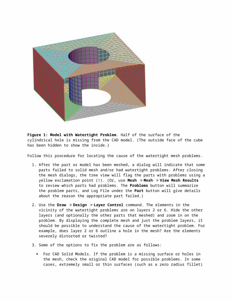
Construction Vertices - Seed Points

A modeling situation may occur which requires a node to be located at a specific position. Some examples of this type of situation are the following.

A load or constraint will be applied to the model at a specific location.

Additional elements, such as actuators, beams or pulleys, will be connected to a CAD solid model at a specific location.

The results must be calculated at a specific location.

These situations will require the addition of seed points to the model. Seed points must be placed on the surface of the CAD solid model. A seed point can be added using two methods.

If the X, Y and Z coordinates of the seed point location are known, select Draw Draw Construction Vertex. This will access the Define Construction Vertex. Specify the X, Y and Z coordinates and press the <Enter> key. The seed points will be represented on the model as a small blue square.

Once a mesh has been created, a vertex can be selected. A seed point can be added to a selected vertex by right-clicking and selecting Add Construction Vertices. This method will also allow you to specify a seed point at a location relative to the selected vertex. For example, if you want a vertex to be located 2.5 inches from a corner of a part, you can select the corner node, right-click, select Add Construction Vertices. Then, enter the relative distance from the corner. The model must be meshed again for the vertices to be located at the seed points.

Seed points can be removed from a model by selecting them in the display area, right-click and select the Delete command (or press the <Delete> key).

Fluid Generation

The Fluid Generation command allows you to create solid parts based on features from the existing CAD geometry. Although this feature is most often used to model fluid flowing in or around the CAD geometry, it is not limited to fluid flow models.

There are two capabilities of the fluid generation. The first is to create internal geometry. This would be used to create a part for a fluid flowing through a tube. The second use is to create external geometry. This would be used to create a part for air flowing around a part.

NoteFor the fluid generation command to be available, the model must be imported into Autodesk Simulation with surface knitting, even if the model is a single part. See the Knit surfaces on import options on the CAD Import tab of the Tools: Options dialog.

Fluid Generation is not available for models originating from Rhino files.

Internal

To define the internal volume from which a part will be created, you must specify two parameters. The first is any single surface on the interior of the current geometry that will be used to create the new part. The software will be able to determine the rest of the surfaces that make up the internal part. Click this surface in the display area and press the Select button in the Interior surface section.

The second parameter is the bounding surfaces. The bounding surfaces must be planar surfaces that share an edge with the interior surfaces of the part. Each bounding surface must contain an entire hole. The edges where the bounding surfaces meet the interior must define a single enclosed volume for the part to be generated successfully. Select each bounding surface and press the Add button to add it to the list. Once all of the bounding surfaces have been selected, press the OK button to generate the part.

For example, refer to the part in the following figure. If we want to create a part representing volume which could occupy, or fill, the hole, we would select either of the semi-cylindrical surfaces (A or B) as the interior surface. Then, we would select the top and bottom surfaces (C and D) as the bounding surface.

External

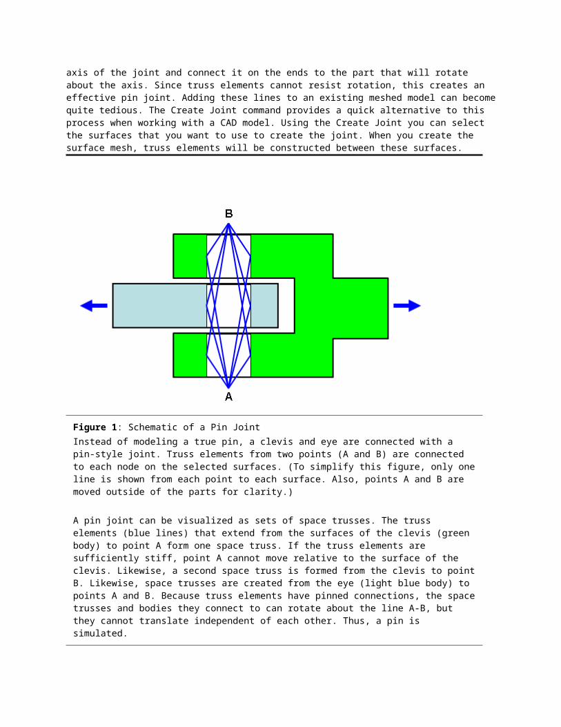
To generate a part for the external area around a model, you must define rectangular prism around the part. When the External command is selected, the Generate Fluid Exterior dialog will appear with default values based on the dimensions of your model. A diagram in the dialog shows how the parameters correspond to the display area. You can alter the center point and the lengths of the prism edges by changing the values in the appropriate fields. A transparent prism will appear over the model in the display area to reflect the part that will be created. The prism must enclose the model. A side of the prism cannot intersect part of the model. Once the desired prism is defined, press the OK button to create the part. A single continuous volume will be generated. For example, if you have a square tube with plates welded to both ends and generate the external fluid, the volume inside the tube will not be included. If this area is desired, you must use the Internal command. However if one of the ends of the tube is not closed, the area inside the tube will be included in the external fluid part.

Parts created using the Fluid Generation can be modified or deleted from the model by right-clicking on the heading for that part in the tree view and selecting either the Modify or Delete command.

Perform Mesh Studies A common question in FEA is what mesh size is required to get accurate results. When working with a CAD model, the Mesh Study Wizard can be used to answer that question. The Mesh Study Wizard automates the task of meshing the model at different mesh sizes, performing the analysis, and querying the results.

Set up the model

Before performing the mesh study, you must first perform the following steps:

1. Open the CAD model in Autodesk Simulation.

2. Set the analysis type to Static Stress with Linear Material Models.

3. Set any special meshing options such as the type of mesh (solid, midplane, plate/shell), refinement points, mesh matching tolerance, and so on.

4. Add surface, edge or part loads and constraints to the model. Nodal loads applied to the CAD parts will not be retained during the study.

5. Optionally, mesh the model.

6. Define the Element Definitions.

7. Define the Material properties.

8. Define the Analysis Parameters.

9. Optionally, do a Check Model or perform the analysis.

10. Exit from the user interface and save the model. Tip

Although the model does not need to be meshed before hand, we recommend to do so to reveal any problems with the model and setup.

If adding refinement points, consider using a Divide factor type instead of a Mesh size type. This way, the mesh around the refinement will always be a factor smaller than the overall mesh size instead of being the same size in all iterations. (See Refinement Points for details.)

Although it is not necessary to do a Check Model or perform the analysis, it is recommended to do so to uncover any problems with the model and setup.

Set up the mesh study

Access the Start Programs Autodesk Autodesk Simulation Tools folder and select the Mesh Study Wizard command. Note that the version number of Autodesk Simulation may be included on the Start Programs menu.

Press the Next button to begin the setup.

Select a model: Press the button and navigate to the location of the model. The model must have at least one design scenario with a Static Stress with Linear Material Models analysis type. Press the Open button to load the model. Press the Next button to proceed. NoteOnly one mesh study is allowed for a model.

Select a design scenario: Select the design scenario which will be used for the mesh study. Only design scenarios with the Static Stress with Linear Material Models analysis type will be available. Press the Next button to proceed. Note that the selected design scenario is not altered in the model.

Mesh size: This step is used to set what size meshes to use for the study.

Specify the type of mesh size control that you want to use in the Type drop-down box. The Percent of automatic and Absolute mesh size options are available. (Refer to the page Model Mesh Settings: Surface for information on these options.)

Specify the limits of the mesh size in the Start size and End size fields.

Specify how many analyses will be performed in the Total iterations field. The difference between the start and end mesh sizes will be divided into equal segments using the total iterations value. For example, two iterations would perform the analysis at the start and end size, three iterations would perform one additional analysis with a mesh size half way in between, and so on.

Press the Next button to proceed.

Define the results: This step is used to set what result is recorded for each analysis, and loosely where the result occurs. When the design study finishes, a graph of the mesh size versus the result will be displayed.

Two types of results are available in the Location drop-down box: Element Node and Node. Element Node results are element-based results in which the result is given at

every node in every element; consequently, each node will have multiple results when shared by multiple elements. This type of result includes stress and strain results. Node results are nodal-based results in which the result is given only at the nodes. This type of result includes displacement and reaction forces.

Select the basic result type that you want to be recorded in the Output Calculation drop-down box. The available options will depend on the selection in the Location drop-down box. Further manipulation of the basic result type can be performed by using the next two drop-downs. For example, to get von Mises stress, or maximum principal stress, the basic result type to select in the Output Calculation would be Stress Tensor.

Select the operation which will be performed on the results type in the Unary Operator drop-down box. This operation will take a vector value (such as a stress tensor) and result in a single scalar value (either by extracting one component of the vector value, or by performing a calculation that results in a scalar value). Therefore, if a scalar result is selected in the Output Calculation, no option will be available in the Unary Operator. If the strain tensor or stress tensor is selected, the operators available will result in the individual tensors, von Mises, Tresca or principal values. If a node result is selected, the operators available will results in one of the X, Y or Z components or the magnitude.

Specify which value from the entire model will be recorded in the Aggregator drop-down box. The mesh study will record one single result from the entire model for each analysis. For example, choose the maximum result or the sum of all results.

NoteThe Element Node results use the unsmoothed values. See the page Results: Results Environment for a discussion of element-based and nodal-based results, smoothed and unsmoothed results.

Run the mesh study

Press the Finish button on the wizard to proceed. The wizard will show the progress of generating the new design scenario, meshing, performing the analysis, and so on. Each step of the process does all of the iterations before starting the next step. That is, all of the new design scenarios are created first (progress bar proceeds from 0 to 100%), then all of the new design scenarios are meshed (progress bar proceeds from 0 to 100%), then all of the new design scenarios are analyzed (progress bar proceeds from 0 to 100%), and so on.

View the results

When the mesh study completes, a graph of the result versus the mesh size will be shown. Right-click in the graph window to perform various graphing functions, such as customizing the layout, saving the graph to an image, and so on. (The graph behaves the same as the graphs in the Results environment, so if you are familiar with customizing and exporting those graphs, the mesh study graphs will be the same.)

Also, the results of each analysis are saved in the model as new design scenarios. Open the model in Autodesk Simulation and load in the appropriate design scenario to review the input and results.

Display the results graph

Once a mesh study has been performed, the graph of the results can be displayed as follows:

1. Use My Computer to show the contents of the folder containing the model.

2. Use another My Computer window to show the contents of the Autodesk Simulation installation folder (such as C:\Program Files\Autodesk\Autodesk Simulation followed by the version number of the software).

3. Drag the file modelname.msw from the first window and drop it onto the program MeshStudyViewer.exe in the second window.

Create and Modify Geometry in the FEA Editor In the FEA Editor environment, you use commands on the Draw tab to create and modify geometry. Click the link to the menu that you need more information about. NoteThe FEA Editor prevents identical lines from being created, where identical means that the lines have the same end points and are on the same part number. Whether two end points are the same or not is determined by the values you specify in the Draw ModifySet Search Tolerance dialog box. This rule has an effect when adding geometry, copying, meshing, and so on.

Topics in this section Drawing Planes Add Geometry Modify Geometry Inquire Utilities Modify Autodesk Inventor Parameters

Drawing Planes Drawing planes are used to add geometry to the model. Instead of the freedom of adding the geometry in 3D space, the geometry is always snapped into the plane. In addition to the obvious advantage of being able to draw flat geometry, regions created with construction objects drawn in a plane can be meshed with the 2D mesher. See the page Meshing Overview: Meshing Hand-built Models: 2D Mesh Generation for details.

When using a drawing plane, the FEA Editor environment is in sketch mode. Hence, the terminology sketch and drawing plane will be used interchangeably.

Create a plane

Additional planes can be created by using Draw Draw New Sketch Plane, or by right-clicking on the Planes branch of the tree view and choosing New Plane.

You can select between the three planes parallel to the global axes (XY, YZ or XZ). You can also select the Advanced option or the 3 points option to define an off-axis plane. Activating the Use Offset check box will allow you to offset one of the global planes from the origin. A positive offset places the plane in the positive direction. For example to draw in the X=10 plane, select the YZ option, activate the Use Offset check box and type 10 in the adjacent field.

Enter, use, and exit Sketch Mode

To enter sketch mode to draw on a plane, right-click the desired drawing plane in the tree view and choose Sketch. When in sketch mode, a grid will appear in the display area and the drawing plane is shown in bold in the tree view. All sketching will be done in this plane. The grid can be turned off by right-clicking on the plane in the tree view and clearing Visibility. The spacing of the grid can be customized on the Options Sketching tab.

Geometry is added to the sketch just like any other geometry: use the commands on Draw and Design panel of the Draw tab. All properties such as part, surface, and layer number, and any object-specific input, are used in the sketch mode just like it is in the 3D mode. (See the page Adding Geometry for details.) The only real difference between adding these objects in 3D mode versus adding them in sketch mode is whether the entered points snap to the drawing plane or not.

When drawing sketch entities, if the cursor is close to a grid point, a lock icon will appear on the cursor. If you click, the item you are drawing will be snapped to that grid point. Likewise, you can snap the new geometry to existing geometry. The points will be projected into the drawing plane.

When an item is added to a sketch, a branch is created under the appropriate part that lists the drawing plane, and this branch includes an entry for each item drawn in that sketch. Click the drawing plane entry under the part to highlight the corresponding items.

To exit sketch mode, right-click the drawing plane and deactivate Sketch. Also, activating the sketch mode for another plane will deactivate the sketch mode for the current plane.

Copy between sketches

Here are the ways to copy items or sketches to other sketches:

Change Plane. All construction objects assigned to a sketch (the Plane entry in the tree view listed under the part) can be moved or copied to a different plane. Right-click the sketch entry and choose Change Plane. The Transfer to Different Plane dialog will appear and list the available planes in the Target Plane drop-down. (If necessary, create the new target plane beforehand using Draw Draw New Sketch Plane.) If the Copy to target plane option is not activated, the selected sketch will be moved to the target plane. When the two planes are parallel, the move

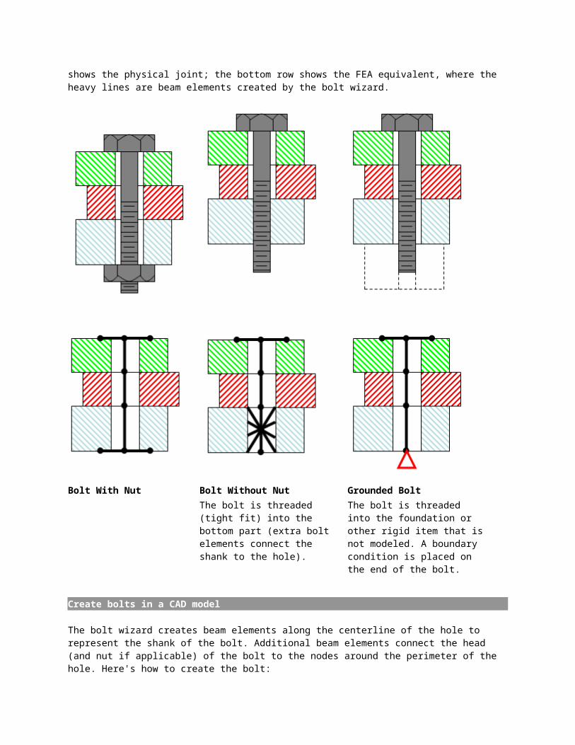
or copy operation is straight forward. When the two planes are not parallel, then the transformation may be harder to visualize (but is still straight forward). The 3D coordinates of each object are converted or projected to local (U,V) coordinates within the existing sketch. The objects are placed in the target plane with the same (U,V) coordinates, then converted to 3D coordinates. So, if a construction line is from (0, 3, 4) to (0, 6, 8) and sketched in the global YZ plane, it would parameterize as a line from (3,4) to (6,8) in (U,V) space. These same (U,V) coordinates in the global XY plane would transform to a line from (3, 4, 0) to (6, 8, 0) in 3D space. Note that the part, surface, and layer number of the construction objects are not changed, so the branch for the new sketch appears in the same part as the original sketch.

Copy and Paste. Individual construction objects in one sketch of a part can be copied (or cut) and pasted into the same sketch plane in another part. Select the objects (either in the tree view or in the display area), right-click and choose Copy or Cut. Then select the target sketch plane in the tree view, right-click, and choose Paste. Also, you can drag the entries from the sketch in one part to the same sketch plane in another part and drop them into the sketch. Naturally, this operation requires that the target sketch exists in the target part. Other than changing the part number of the copied object, the surface and layer number remains the same.

NoteIf a construction object in a sketch is selected and changed with the Draw Pattern Move or Copy command, then the object is no longer associated with a sketch. It

becomes a 3D Object and is listed in a separate branch under the part.

Convert from 3D objects to a sketch

There are situations in which a construction object is not in a drawing plane, so the tree view lists the item as a 3D object. Some commands are not available on 3D construction objects, such as 2D meshing. These 3D objects can be copied to a sketch as follows:

1. Select the 3D construction objects with the Selection Select Construction Objects command.

2. Copy or cut the objects to the clipboard. Right-click and choose either Cut or Copy.

3. Activate the drawing plane into which the objects should go. (Right-click the appropriate plane under the Planes branch of the tree view and choose Sketch.)

4. Paste the 3D objects into the part. Right-click the part name in the tree view and choose Paste. Note that the object must be pasted into a sketch on a different part than the original objects.

Note that the original 3D construction object is not projected into the drawing plane. Therefore, the object should lie in the plane into which it is being pasted.

Calculate the properties of a sketched region

The cross sectional properties of a sketch can be calculated. The guidelines for the sketch or sketches are as follows:

Draw the region to be calculated using construction objects.

Draw the objects while in sketch mode.

The objects can be in different parts but need to be in the same drawing plane. The combination of all parts on all selected sketches will define the region or regions.

Any drawing plane can be used. The results will be in the local coordinates of the plane.

The sketch must enclose an area or multiple areas.

Holes within the area are permitted.

Regions can overlap, in which case the overlap region is calculated as if it were a hole, but separate regions should not touch. See the following figure.

(a) Two overlapping regions (above) are supported by the 2D Moment of Inertia. The overlapping region between the square and the circle becomes a hole in the cross section. The calculations are based on shaded the regions (below).

(b) Two regions that do not overlap (above) are not supported by the 2D Moment of Inertia. The problem areas are identified with the inverted triangles (below) when the command is executed. To calculate this area, remove the line in common between the square and the semi-circle. (Alternatively, a duplicate line - one for the square and one for the semi-circle --- could be used. For example, the duplicate would be required if the square and semi-circle were on separate parts and the two regions were going to be meshed with the 2D mesh engine.)

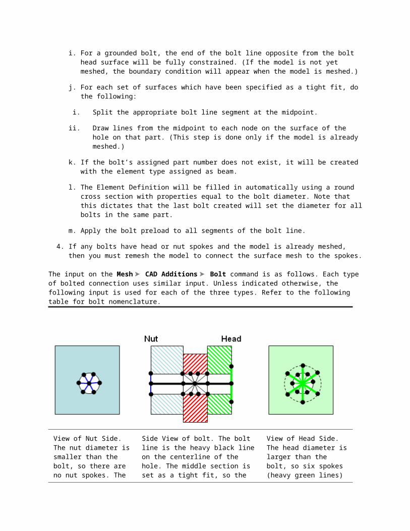
Once the sketches are made, either select the plane in the Planes branch of the tree view or select the plane entries in the tree view under the part, then right-click, and choose 2D Moment of Inertia. Selecting the Planes branch is equivalent to selecting each of the individual planes appearing under each part. The calculator will split the combined sketches into a series of horizontal rectangular strips and perform a numerical integration based on these strips. The results are given in the 2D Moment of Inertia Results dialog and consist of the following:

Area

Center of Gravity location, given in local coordinate system of the plane (u,v). The global coordinates of the center of gravity can be determined by inquiring on the construction vertex that is added to the model.

Area moment of inertia about the horizontal and vertical axes of the plane (u and v axes) passing through the center of gravity of the sketch. The orientation of these axes is given as a vector in global coordinates in the Local Orientation

A construction vertex is also added to the model at the location of the center of gravity. TipThe accuracy of the calculation depends on the number of divisions used to split the sketch into rectangular strips. The height of the sketch (in the v direction) is divided into the number of divisions specified under the Options Sketching tab.

The Save Results dialog will appear when the Save button is clicked. Choose the file name and location of the area calculation results. Activate the Append check box on the Save Results dialog before clicking the Save button to append the current results to an existing file. Otherwise, the existing file will be overwritten with the current results.

Similar calculations can be performed on fully meshed models by using the Analysis Analysis Weight and Center-of-Gravity command. See the page General Options: Weight and Center of Gravity Calculator.

Add Geometry

The commands on this page are accessed from the Draw and Design panels on the Draw tab.

Common Items

When geometries --- such as lines, arcs, circles --- are added to a model, the objects can be of two different types:

Use as Construction When this box is activated, the added geometry object is not part of the mesh. Instead, it is used as an aid to build a mesh (either an automatic 2D meshed region, or structured mesh, both described later). For example, four construction lines connected together to form a rectangle do not create a plate element when the analysis is performed. Construction arcs, circles, and splines are shown as their theoretical smooth objects. Construction objects are listed in the tree view either under the drawing plane/sketch branch or under the <3D Objects>

branch, from which the objects can be modified (change the coordinates of the defining points, change the attributes, and so on). (See the page Drawing Planes for the distinction between a drawing plane/sketch and a 3D object, and for methods to move an item from 3D space to a sketch.)

Regular Lines: When the added object is not a construction object, it will be used as part of the mesh. For example, four lines connected together to form a rectangle do create a plate element when the analysis is performed. Since the objects are part of the mesh, non-construction arcs, circles, and splines are immediately divided into straight line segments when they are added to the model. That is, the arcs and circles are meshed. See the page Tools: Modify Attributes and Duplicate for instructions on changing an item from a construction object to a regular line and vice versa.

When adding geometry, the points can be entered with any of these methods:

Enter the X, Y, and Z coordinates of the point in the respective fields and press <Enter>. If the Use Relative check box is activated, the values entered in the DX, DY, and DZ fields will specify the relative distance in those directions from the current coordinate (shown in the status bar). For example, if the from point is (X=10, Y=5, Z=2.5) and you type ---1 in the DY: field and 2.5 in the DZ: field, a point will be defined at (X=10, Y=4, Z=5) instead of (X=0,Y=-1, Z=2.5).

Snap to an existing point. Move the cursor to the point where you want to begin; once the lock icon appears (see image below), left click the mouse to select that vertex.

If using sketch mode, left click the mouse to snap to a grid point or at any free-hand position on the plane.

Enter the vertex ID of the vertex in the model at which you want to begin the line in the ID: field. The vertex ID of a vertex can be determined by hovering the cursor over a point. A pop-up will appear with the vertex ID as shown below.

Add a New Part to a Model

New Part: Selecting this command adds an empty part with the next available part number. Any type of geometry can be added to this part.

Add Construction Nodes to a Model

Construction Vertex: Use this command to add a vertex (node) to the model. Construction vertices have two purposes:

1. Used as a reference point to add hand-built geometry to the model, such as lines, arcs, meshes, and so on. This vertex will not be included when the model is analyzed (unless of course an element is connected to the vertex).

2. When working with a CAD solid model, construction vertices will force the surface mesher to create a node at that location. Refer to the page Meshing Overview: Meshing CAD Solid Models: Construction Vertices -Seed Points for details.

The Define Construction Vertex dialog will appear.

Enter the coordinates where you want the construction vertex to be added.

Press <Enter> to add the vertex. TipUse View Appearance Construction Vertices to display or hide the construction vertices.

Add Lines to a Model

Line: Use this command to add a line segments to the model. This segments can be defined as any line element.

1. The Define Geometry dialog will appear.

2. First specify the part, surface and layer to which the lines will be assigned in the Attributes section. The lines can be placed in any surface or layer number.

3. Specify the beginning coordinate for the line using one of the above methods in Common Items. If you move the mouse, you will see that the cursor is rubberbanded to the endpoint.

4. Specify the second endpoint of the line. You will see the line appear in the viewing area.

5. You can continue to add more lines in this dialog. You can either continue from the last endpoint, or can start a separate line. This can be controlled by the Single Line check box.

To enter a series of line elements that are connected together to form a continuous chain, make sure that the Single Line check box is deactivated.

To define separate lines that do not connect together, make sure that the Single Line check box is activated.

NoteThe FEA Editor prevents identical lines from being created, where identical means that the lines have the same endpoints and are on the same part number. Whether two endpoints are the same or not is determined by the Draw Modify Set Search Tolerance dialog. This rule has an effect when adding geometry, copying, meshing, and so on. TipWhen adding lines, the default of creating a construction object or a regular object is determined by the setting Add lines defaults to construction lines on new file open located on the Options Sketching tab.

Generate Tangent Lines

Selecting the Tangent Line command guides you through the process of creating tangent lines between construction circles and arcs. This command will only be available if an arc or circle exists in the current sketch. Following the prompts in the status bar, the tangent lines are created as follows:

1. Click the first object for the tangent: either a construction vertex, circle, or arc.

2. Click the second object for the tangent: either a construction circle or arc (or vertex if the first object was not a construction vertex). All possible tangent lines between the two objects will be shown.

3. Select each possible tangent line that you want in the model. Use the <Ctrl>, <Shift> and <Ctrl>+<Shift> to toggle, add, and subtract lines to the selection set.

4. Press the <Enter> key after selecting the desired lines. Construction lines will be created at the selected tangent lines.

Add Rectangles to a Model

Rectangle: Use this command to add four line segments that define a rectangle.

1. The Add Rectangle dialog box appears.

2. First specify the part, surface and layer to which the lines generated from the rectangle will be assigned in the Attributes section.

3. If not in sketch mode, then four points will be required to define the rectangle. If in sketch mode, only the two diagonally opposite points are required. Each of these points can be entered as described above in Common Items. The four points are as follows:

The first point defined must be a corner of the rectangle.

The second point defined must be the corner of the rectangle opposite to the first point.

The third point defined can be any point that lies in the plane of the rectangle. This point cannot lie along the diagonal defined by the first two points.

The fourth point defined can be any point on the base of the rectangle.

4. Press the Apply button to create the line segments.

5. For example, to create a 10 x 10 rectangle at the origin in the XY plane at Z=0 and sides parallel to X and Y, you would use the following coordinates for the four points:

(0,0,0) for the first corner

(10,10,0) for the opposite corner

(2,3,0) or any coordinate where the X and Y values are unequal (so that they are not on the diagonal) and Z=0.

(1,0,0) or any coordinate along the X axis, except for (0,0,0).

Add Arcs to a Model

Arcs can be added in 3D space using Arc Three Points or Arc Center and Endpoints. When in sketch mode, arcs can also be entered by specifying the Angle and Endpoints or Radius and Endpoints.

1. The Define Arc using dialog will appear.

2. First specify the part, surface and layer to which the arc (or lines) will be assigned in the Attributes section.

3. If not creating a construction object, specify how many line segments into which the arc will be divided in the Minimum Segments: field. The segments will be of equal length. To control the lengths of the lines create from the arc, activate the Maximum Length: check box and specify the maximum length of the line segments that will be generated in the adjacent field. If the length of the arc divided by the value in the Minimum Segments: field is greater than this value, more segments will be generated than specified in the Minimum Segments: field.

4. Define the points for the arc, following the prompts in the status bar. Each of these points can be entered as described above in Common Items.

5. For some arc commands that have a direction, activate the Reverse Sense of Arc check box to have the other section of the arc displayed.

6. Press the Apply button to create the arc or line segments.

Add Circles to a Model

Circle Diameter or Circle Center and Radius: Use these commands to add circles to the model.

1. The Define a Circle by Diameter Points or Define a Circle by Center and Radial Point dialog will appear.

2. First specify the part, surface and layer to which the lines generated from the circle will be assigned in the Attributes section.

3. If not creating a construction object, specify how many line segments into which the circle will be divided in the Minimum Segments: field. The segments will be of equal length. To control the lengths of the lines create from the circle, activate the Maximum Length: check box and specify the maximum length of the line segments that will be generated in the adjacent field. If the circumference of the circle divided by the value in the Minimum Segments: field is greater than this value, more segments will be generated than specified in the Minimum Segments: field.

4. Define the points for the circle, following the prompts in the status bar. Each of these points can be entered as described above in Common Items.

5. Press the Apply button to create the line segments.

Add Splines to a Model

Spline Curve: Use this command to add splines to the model.

1. The Add Spline dialog will appear.

2. First specify the part, surface and layer to which the lines generated from the spline will be assigned in the Attributes section.

3. If not creating a construction object, specify how many line segments into which the spline will be divided in the Minimum Segments: field. The segments will be of equal length. To control the lengths of the lines create from the spline, activate the Maximum Length: check box and specify the maximum length of the line segments that will be generated in the adjacent field. If the length of the spline divided by the value in the Minimum Segments: field is greater than this value, more segments will be generated than specified in the Minimum Segments: field.

4. Specify the degree of curvature that will be used to generate the spline in the Degree: field.

5. If you want the spline to pass through all of the defined points, activate the Interpolate check box.

6. If you want the first and last point to be connected, activate the Close check box.

7. Define the points that will be used to generate the spline. Each of these points can be entered as described above in Common Items.

8. Press the Apply button to create the spline or line segments.

Add a Pulley Element

Pulley: This command is available only in a nonlinear analysis. See Pulley Elements for more details.

Add Contact Elements to a Model

Contact Elements: This command will add numerous lines between two sets of vertices on the model. The main use for this command is to create contact or gap elements between every node in one area and every node in another area. But since the command simply creates lines, the lines can be used for any purpose and any element type.

The steps for using the command are as follows:

1. After this command is started, select one of the two sets of vertices in the display area, such as one of the faces for contact. You can use any selection method to select any type of object. For example, if you select an entire part or surface, all of the vertices on that part or surface will be included. If you select a line, both vertices will be selected. Construction vertices can also be selected, but other construction objects cannot be selected.

2. Press the Assign Set 1 button. The number of vertices selected will be listed.

3. Select the second set of vertices to connect, such as the second contact face.

4. Press the Assign Set 2 button. The number of vertices selected will be listed.

5. Specify the attributes of the lines in the Part, Surface and Layer fields.

6. Press the Create Lines button to create the contact elements. Every vertex in the first set will be connected with a line to every other vertex in the second set.

In some situations, you may only want contact elements to be created between nodes that are a certain distance apart. For example, if you know that a part is only going to move 1 inch relative to another part, you do not need contact elements longer than 1.5 inches (leaving a little leeway). This can be done by activating the Constrain lengths check box and specifying the minimum and maximum lengths. Then, only lines whose length is within the constraints will be created when the Create Lines button is pressed.

Layer Control

Layer Control: Displays lines according to the layer attribute (layer number) and filters the lines for easier selection. The dialog box shows all the layer numbers in the model, regardless of part. Select Show to display all the layers in the model. You can also select to show individual layers. For selection, activate Filter to prevent the object from being selected. Filtering works on any type of object: part, surface, edge, line, and vertex. If the object belongs only to lines on a layer that is filtered, then the object is not selected.

Connect Lines to the Centroid

Centroid Creator: The general purpose of this command is to calculate the centroid location of a surface (composed of one or more surface numbers), and optionally connect the nodes on the selected surface to the centroid with line elements. When used on two separate surfaces, the two centroids can be connected with a line element.

For example, consider a long channel used in a structure, and the interaction of the bolted connections at each end are to be studied in detail. So a CAD model of the beam, bolts, and connection is created. If the span of the channel is not of interest in the analysis, it can be replaced with a few beam elements to greatly reduce the size of the analysis. The Centroid Calculator automates the process of connecting each node on the cut end of the channel to the centroid, and then connecting the two centroids. See the following figure.

(a) Full CAD model in which the entire horizontal channel is modeled with brick elements.

(b) More efficient model in which a portion of the horizontal channel is modeled with beam elements. Only the portion requiring the detail provided by brick elements is modeled in the CAD.

The steps for using the command are as follows:

1. Optionally, select the surface numbers on the first surface (Selection Select Surfaces).

2. Activate the Draw Design Centroid Creator command. If any surfaces were selected, they will be listed in the Centroid surface box.

3. Additional surfaces can be selected in the display area and listed in the box by clicking the Add button. Undesired surfaces can be removed by selecting the surfaces in the box and clicking the Remove button.

4. If you want each node on the surface to be connected to a point at the centroid, activate the option Connect centroid to surface with spokes. Indicate which part number to use for the lines with the Part input field. Note that this option requires the model to be meshed ahead of time.

5. If you have a second surface for which you want to calculate the centroid and connect it to the first surface with a line element (such as the example in Figure 1), activate the Connect centroid to second surface centroid option. Then, select the surfaces for the second surface and click the appropriate Add button.

6. Click the OK button to perform the operations. Note

The Centroid Creator only works on surfaces of CAD models. The calculation of the centroid is not dependent on the mesh size.

For all options chosen on the dialog, a construction vertex is placed at the centroid of the surface. If the model is re-meshed, and if the construction vertex is near the surface of the model, a node will appear in the CAD mesh at the centroid location. See the page Meshing Overview: Meshing CAD Solid Models: Construction Vertices -Seed Points for details. If this is not desired, select the construction vertex (Selection Select Vertices) and delete it before re-meshing.

The centroid spokes are not associative with the model, so if the model is re-meshed, the old centroid spokes should be deleted, and the centroid spokes should be re-created with the new surface mesh.

Modify Geometry

You can use commands on the Draw tab to modify existing objects. Keep in mind that the objects can be of two different types:

Use as Construction: When this box is activated, the added geometry object is not part of the mesh. Instead, it is used as an aid to build a mesh (either an automatic 2D meshed region, or structured mesh, both described later). For example, four construction lines connected together to form a rectangle do not create a plate

element when the analysis is performed. Construction arcs, circles, and splines are shown as their theoretical smooth objects. Construction objects are listed in the tree view either under the drawing plane/sketch branch or under the <3D Objects> branch, from which the objects can be modified (change the coordinates of the defining points, change the attributes, and so on). (See the page Drawing Planes for the distinction between a drawing plane/sketch and a 3D object, and for methods to move an item from 3D space to a sketch.)

Regular Lines: When the added object is not a construction object, it will be used as part of the mesh. For example, four lines connected together to form a rectangle do create a plate element when the analysis is performed. Since the objects are part of the mesh, non-construction arcs, circles, and splines are immediately divided into straight line segments when they are added to the model. That is, the arcs and circles are meshed. See the page Tools: Modify Attributes and Duplicate for instructions on changing an item from a construction object to a regular line and vice versa.

Some of the commands work on both types of objects, but a few only work on one type. Since most of the commands work on lines or construction objects, the Select mode must be set to Lines or Construction Objects to activate the commands. NoteThe FEA Editor prevents identical lines from being created, where identical means that the lines have the same end points and are on the same part number. Whether two end points are the same or not is determined by the Draw Modify Set Search Tolerance dialog. This rule has an effect when adding geometry, copying, meshing, and so on.

Topics in this section Point Move Divide Intersect Fillet Trim Extend Move, Rotate, Scale, or Copy Mirror Modify Attributes and Duplicate Relocate & Scale Project To Plane Set From Point

Point Move

Activating the command:

Draw Modify Point Move

If vertices are selected, right-click and choose Move.

There are multiple ways to move vertices in the user interface using the Point Move command. Any lines that are connected to the point will remain connected to the point at the new location. (Construction lines can be stretched with the Point Move command, but other construction objects are not affected.)

With nothing selected: This method can be used for moving a single vertex to a new position. The vertex will be selected after the command is executed.

1. Select the Point Move command.

2. Click the vertex that you want to move. The padlock icon will appear on the mouse when you are over a vertex.

3. Specify where you want to move the node. You can either enter the coordinate of the new location or activate the Use Relative check box and specify how far you want to move the point in each direction; then press <Enter> to perform the move. Or use the mouse to indicate where to move the vertex to.

4. Another vertex can be selected and move, and so on, without closing the Point Move dialog.

5. Click the Close button after moving all of the desired points.

With vertices selected: This method can be used for moving a single or multiple vertices. This method works on the currently selected vertices.

1. Select the vertices that you want to move.

2. Right-click in the display area and select the Move command.

3. Specify where you want to move the node. You can either enter the coordinate of the new location or activate the Use Relative check box and specify how far you want to move the point in each direction; then press <Enter> to perform the move. Or use the mouse to indicate where to move the vertex to.

4. Click the Close button to close the dialog.

Divide


Draw Modify Divide

If lines or construction objects are selected, right-click and choose the Divide command.

Selecting the Divide command will access the Divide Lines dialog. (This can really divide any object: lines, arcs, circles, and so on.)

1. Select the lines or construction objects that you want to divide into multiple segments.

2. Select the Divide command.

3. Type in the number of lines that you want to divide each of the selected items into in the Number of Lines field. You can also use the up and down scroll buttons to specify the number of lines. If you have multiple items selected, each item will be divided into this many divisions.

4. Press the OK button. The items will now be divided into the specified number of equal length objects.

The Divide command works on regular lines and construction objects. Construction objects are divided into smaller construction objects, so construction circles and construction arcs are divided into smaller construction arcs. To create regular lines from the construction circles or arcs, use Mesh Structured Mesh Divide 1 Object.

Intersect


Draw Modify Intersect

If construction objects are selected, right-click and choose the Intersect command.

If in Selection Select Lines or Selection Select Construction Objects mode, then choosing the Intersect command will access the Intersect lines dialog. (This can really intersect any object: lines, arcs, circles, and splines.)

Note that two sets of selections will need to be made on the fly. You do not need to make the selections before activating the command. The two selection sets are as follows:

1. Select the single item or multiple items that are used to create the intersection.

2. Then, select the single item or multiple items to be intersected.

The objects can be lines or construction objects or a mix of both. When using a mix, the Select setting will need to be changed in the middle of the operation.

The procedure to intersect objects is as follows:

1. Activate the Intersect command and follow these prompts:

2. Select an intersecting line indicates to select the first item that will be used to intersect the other items.

3. Select another intersecting line or Press ENTER to select lines to intersect lets you select additional items to create the intersection. Pick each item one at a time by left clicking on the line regardless of the Selection: Shape setting.

Press the <Enter> key when all of the items being used to create the intersections are selected.

4. Press ENTER to perform the intersection or select another line to intersect indicates to select the first item to be intersected. Regardless of the Selection Shape setting, you need to left click the item to select it. To select multiple objects to be intersected, you must pick them one at a time by left clicking on them.

Press the <Enter> key to perform the intersect operation.

Only objects that are in the same plane can be intersected. However, they do not need to physically cross. If the Use equation of the intersecting entity check box is activated, the equation of the object will be used for the intersection. That is, the object is treated as if infinitely long.

If the Intersect all other lines check box is activated, you will only need to select the objects to create the intersections; not the objects to be intersected. All of the entities that the selected object intersect will be intersected when the <Enter> key is pressed.

Fillet


Draw Draw Fillet

If lines or construction objects are selected, right-click and choose Fillet.

Naturally, the items need to be in the same plane to create the fillet.

1. Select the Fillet command.

2. Type the radius of the fillet in the Radius field.

3. If you want the fillet to be created as line segments, make sure the Use as Construction is not activated. Then specify how many line segments into which the fillet will be divided in the Minimum Segments: field. The segments will be of equal length. To control the lengths of the lines created from the fillet, activate the Maximum Length: check box and specify the maximum length of the line segments that will be generated in the adjacent field. If the length of the fillet divided by the value in the Minimum Segments: field is greater than this value, more segments will be generated than specified in the Minimum Segments: field.

4. Select each of the two lines to fillet. Select the lines closer to the endpoint on the segment to keep; the endpoint further from the selection click point will be trimmed or extended as needed to satisfy the fillet radius.

5. The fillet will be created when the Apply button is clicked. If Use as Construction is not activated, the fillet and original lines and will be created as regular line segments. If the option is activated, the fillet and original lines will be created as a construction arc and two construction lines.

TipTo trim or extend two lines so that they meet at the same point, create a fillet between the two lines with a radius of 0.

When the analysis type is Nonlinear, the Fillet command has an extra option: Create Pipe Bend. This option is used to create an elbow for the pipe element. For details, see the page Setting Up and Performing the Analysis: Nonlinear: Element Types and Parameters: Pipe Elements.

Trim


Draw Modify Trim

If lines or construction objects are selected, right-click and choose Trim.

Trim will shorten one object to where it is crossed by another object. It will not trim one object into two shorter objects.

The objects can be lines or construction objects or a mix of both. When using a mix, the Selection Select setting will need to be changed in the middle of the operation. Also, the items must be in the same plane.

Follow the prompts in the status bar to work the trim command, as follows:

1. After you select the Trim command, select the object that will be used as the cutting object. This is also referred to as the boundary item.

2. Next, select the object that will be trimmed. The objects must physically cross. That is, the boundary object is not considered to be infinitely long.

3. Next, select the portion of the trimmed object that you want to delete. The trimming operation will be performed.

4. Repeat the trim command for additional objects or press <Esc> to exit the command. TipTo trim or extend two lines so that they meet at the same point, create a fillet between the two lines with a radius of 0.

Extend


Draw Modify Extend

If lines or construction objects are selected, right-click and choose Extend.

Extend will lengthen one object to where it is crosses another object. The objects can be lines or construction objects or a mix of both. When using a mix, the Selection Select

setting will need to be changed in the middle of the operation. Also, the items must be in the same plane.

Follow the prompts in the status bar to work the extend command, as follows:

1. After you select the Extend command, select the object that will be used as the extend to object. This is also referred to as the boundary item.

2. Next, select the object that will be extended. The objects must physically cross for the command to succeed. The boundary object is not considered to be infinitely long. If the object being extended is an arc, you are prompted for which end of the arc to extend.

3. Repeat the extend command for additional objects or press <Esc> to exit the command.

TipTo trim or extend two lines so that they meet at the same point, create a fillet between the two lines with a radius of 0.

Move, Rotate, Scale, or Copy Activating the command:

Draw tab Pattern panel

If lines or construction objects are selected, right-click and choose command.

The operation of moving, rotating, scaling, and copying items are combined on one dialog. Choosing Move or Copy or Rotate or Copy or Scale or Copy will let you do any or all of the other operations.

1. Select the lines and/or construction objects that you want to perform the operation on. FEA objects (loads, boundary conditions, and so on) cannot be altered with these commands.

2. Select the appropriate command.

3. The Operation section of the Move, Rotate, Scale or Copy dialog will have the check box activated for the operation you selected. To perform more operations, activate the appropriate check boxes.

4. To create copies of the selected lines during the operation, activate the Copy check box. If you want the copies to be joined, activate the Join check box. Lines will be drawn from the endpoints of the original lines to the endpoints of the new lines, and construction objects will be drawn from the endpoints of the original construction objects to the endpoints of the new construction objects. Specify how many copies you want to create in the adjacent field.

5. To also move the ends of lines that share an end point with the selected line, activate the Move Ends check box.

6. If you are performing a move operation, specify how far you want to move the lines in the Total distance field in the Move tab. If you are creating copies, you can either specify this distance or the distance for each copy in the Incremental distance field instead. The other field will be filled in based on how many copies are selected. Select the coordinate system in which the move will be made in the Coordinate system

drop-down box. Specify the direction you want to move the objects in the Direction vector section. Either select the radio button for the global direction, or select the Custom radio button to specify a vector. You can also press the Vector Selector button to define a vector by selecting two vertices in the model. If you want the move to be performed in the opposite direction of the vector, press the Reverse Direction button.

7. If you are performing a rotate operation, specify the total angle through which you want to rotate the lines in the Total angle field in the Rotate tab. If you are creating copies, you can either specify this angle or the angle for each copy in the Incremental angle field instead. The other field will be filled in based on how many copies are selected. You can also press the Select Total Angle button to select three vertices in the model to define the rotation angle. The first vertex will be the origin of the angle. The second point will define the start point of the angle. The third point will define the end point of the angle. Specify the axis about which you want to rotate the objects in the Rotation axis section. Either select the radio button for the global axis, or select the Custom radio button to specify a vector. You can also press the Vector Selector button to define a vector by selecting two vertices in the model. Specify the center point of the rotation operation in the Rotation center point section. You can either enter the coordinates or press the Select Center Point button and select the vertex in the display area.

8. If you are performing a scale operation, select the radio button in the Scale type and factor section to define how you want the scaling to be performed.

Select the Uniform (scale in all three directions) radio button to scale the lines equally in all directions. Specify the point about which you want the lines scaled in the Fixed point section. You can either define the coordinates of the point or press the Select Fixed Point button and select the fixed point in the display area. Specify the scale factor for each scale operation in the Scale factor field. You can also press the Select Scale Factor button and select three points in the display area. The first point will be the fixed point. The second will be the start of the scale factor and the third point will be the end of the scale factor. For example, if you select the points so that the second point is closer to the fixed point than the third point, the scale factor will increase the distance of the selected lines from the fixed point. If you select the points so that the second point is further from the fixed point than the third point, the scale factor will decrease the distance of the selected lines from the fixed point. An example of this scaling method can be demonstrated on a circle that has been divided into several line segments. Select the Uniform (scale in all three directions) radio button and select the center of the circle for the fixed point. If you specify a scale factor greater than one, a set of concentric circles will be generated outward from the original circle. If you specify a scale factor less than one, a set of concentric circles will be generated inward from the original circle.

Select the Perpendicular to (scale in two directions) radio button to scale the lines equally in two directions. Specify the point about which you want the lines scaled in the Fixed point section. You can either define the coordinates of the point or press the Select Fixed Point button and select the fixed point in the display area. Specify the direction of the vector perpendicular to the two directions in which you want the lines to be scaled in the Scale direction vector section. Either select the radio button for the global axis, or select the Custom radio button to specify a vector. You can also press the Vector Selector button to define a vector by selecting two vertices in the model. Specify the scale factor for each scale operation in the Scale factor field. You can also press the Select Scale Factor button and

select three points in the display area. The first point will be the fixed point. The second will be the start of the scale factor and the third point will be the end of the scale factor. For example, if you select the points so that the second point is closer to the fixed point than the third point, the scale factor will increase the distance of the selected lines from the fixed point. If you select the points so that the second point is further from the fixed point than the third point, the scale factor will decrease the distance of the selected lines from the fixed point. An example of this scaling method can be demonstrated on a circle that has been divided into several line segments. The circle lies in the XY plane. Select the Perpendicular to (scale in two directions) radio button and select the center of the circle for the fixed point. If you select the X direction for the scale direction vector, the result will look like ellipses whose axis along the Y direction gets larger or smaller depending on the scale factor. This is because the distance from the X axis will be scaled. If you select the Y direction for the scale direction vector, the result will look like ellipses whose axis along the X direction gets larger or smaller depending on the scale factor. This is because the distance from the Y axis will be scaled. If you select the Z direction for the scale direction vector, the result will look like concentric circles.

Select the Along line (scale in one direction) radio button to scale the lines along one direction. Specify the point about which you want the lines scaled in the Fixed point section. You can either define the coordinates of the point or press the Select Fixed Point button and select the fixed point in the display area. Specify the direction of the vector along which you want the lines to be scaled in the Scale direction vector section. Either select the radio button for the global axis, or select the Custom radio button to specify a vector. You can also press the Vector Selector button to define a vector by selecting two vertices in the model. Specify the scale factor for each scale operation in the Scale factor field. You can also press the Select Scale Factor button and select three points in the display area. The first point will be the fixed point. The second will be the start of the scale factor and the third point will be the end of the scale factor. For example, if you select the points so that the second point is closer to the fixed point than the third point, the scale factor will increase the distance of the selected lines from the fixed point. If you select the points so that the second point is further from the fixed point than the third point, the scale factor will decrease the distance of the selected lines from the fixed point. An example of this scaling method can be demonstrated on a circle that has been divided into several line segments. The circle lies in the XY plane. Select the Along line (scale in one direction) radio button and select the center of the circle for the fixed point. If you select the X direction for the scale direction vector, the result will look like ellipses whose axis along the X direction gets larger or smaller depending on the scale factor. This is because the distance along the X axis will be scaled. If you select the Y direction for the scale direction vector, the result will look like ellipses whose axis along the Y direction gets larger or smaller depending on the scale factor. This is because the distance along the Y axis will be scaled. If you select the Z direction for the scale direction vector, no scaling will occur because all of the lines have the same Z coordinate.

Mirror Activating the command:

Draw Pattern Mirror

If lines or construction objects are selected, right-click and choose Mirror.

To use the Mirror command, follow these steps:

1. Select the lines and/or construction objects that you want to mirror.

2. Select the Mirror command. Depending on whether you are working in a sketch or not effects how the mirror command works.

Working in a Sketch: The Mirror Objects dialog appears. Use the Pick button to choose which line (either a regular mesh line or a construction line) to mirror the selected objects about.

Not Working in a Sketch: Select the existing plane about which you want the lines to be mirrored. If the desired mirror plane does not exist, click the New button and define the mirror plane. (See the page Drawing Planes for details on creating a plane.)

3. By default, the selected objects will be copied when they are mirrored. To move the objects when they are mirrored, activate the Delete original objects check box.

4. Press the OK button to perform the mirror operation.

The mirrored objects created will either be placed in a sketch or placed in 3D space depending on whether they were originally in a sketch and if the mirror operation would keep them in a sketch. If they are mirrored to a sketch, the appropriate drawing plane entry in the tree view under the part will have the new entries for the mirrored objects; otherwise, the new objects will appear in the 3D Objects entry in the tree view under the part.

Modify Attributes and Duplicate


Draw Modify Attributes

If lines or construction objects are selected, right-click and choose Modify Attributes or Modify.

Each item drawn (except for construction vertices and refinement points) are assigned to a part, surface, and layer number. Once the objects are drawn, the Modify Attributes command can be used to change those properties.

Select the lines or construction objects that you want to change. (Selection Select Lines or Construction Objects)

Select the command. If the items are lines the command is Draw Modify Attributes or right-click Modify Attributes (or right-click Duplicate --- see below). If the items are construction lines, the command is Draw Modify Attributes or right-click Modify. If the items are other construction objects, the command is right-click Modify.

Change the fields to the desired values.

Press the OK button to apply this change to the model.

Changing Lines and Construction Lines:

When changing lines or construction lines, the dialog that appears is the Line Attributes dialog. The Line Attributes dialog also includes an option to toggle the selected lines between regular mesh lines and construction objects. Simply activate (check) the Construction object check box to convert the lines into construction lines, and deactivate (clear) the box to convert construction lines into regular lines.

There are two other options on the Line Attributes dialog when the selected items are lines:

Maintain part boundary only has an effect when the part number is being changed and only at the boundary between the existing part and the new part. If the element type for the lines being changed is defined, and if changing the part number of some of the selected lines would leave incomplete elements in the unselected lines at the boundary between the two parts, then activating the Maintain part boundary creates a copy of some of the selected lines so that whole elements are maintained in the original part. The part number of the original lines are changed to the new part number. See the figure below.

Duplicate will make a copy of all of the selected lines on the new part number.

Ten element plate model on part 1 (in green). The lines on five elements are selected and being modified to part 2.

Without the Maintain part boundary option, the fifth element from the left in part 1 is missing the line on the right-side to form a complete element. The missing shading indicates a problem. Part 1 now has four elements and two extra lines; part 2 (in red) has 5 elements.

With the Maintain part boundary option, a duplicate line is created at the boundary, maintaining complete elements in part 1. Each part has five elements.

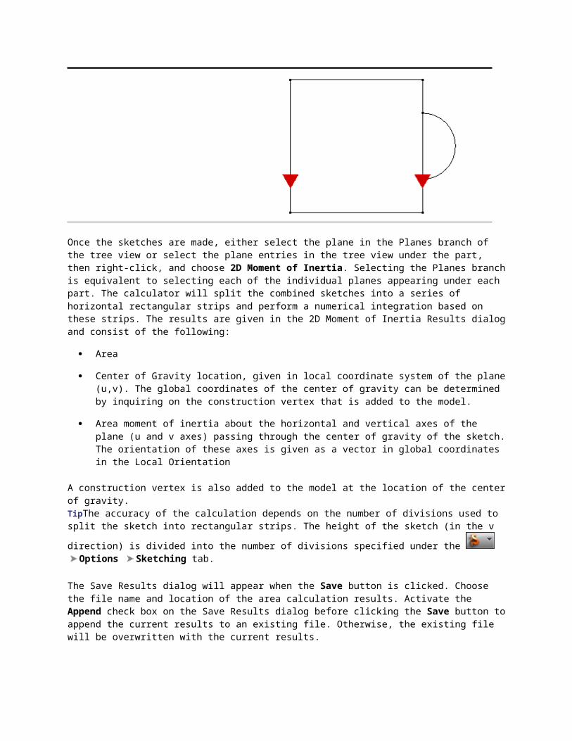
With the Duplicate option, the lines on part 1 are not changed; additional lines are created on part 2. Part 1 has ten elements; part 2 has 5 elements at the same place as part 1. (Further steps are necessary to separate the plate elements if desired.)

Changing Other Construction Objects:

When changing other construction objects (arcs, circles, and splines), there are two different options for changing the objects:

1. The Modify command opens the original dialog window for the type of object. All attributes available when the item was originally created can be changed. In addition to changing the attributes, the points that define the object can be changed. Pressing the <Esc> key will undo through the definition of the points. Then new points can be entered. For example, if a three point arc is defined, pressing the <Esc> key once will undo the definition of the third point on the arc. Thus, the third point can be redefined, or pressing the <Esc> key again will undo the definition of the second point on the arc. Now, the second point can be redefined (followed by the third point), or pressing the <Esc> key again will undo the definition of the first point. Then, all three points can be redefined. NoteEndpoints of arcs, circles, and splines can be changed with the Modify command. The command is only available if a single item is selected. Multiple arcs cannot be changed simultaneously.

2. The Modify Attributes command opens the Line Attributes dialog. As described above (see Changing Lines and Construction Lines:), the part, surface, and layer properties of the selected objects can be changed.

Relocate & Scale

Activating the command: Draw Pattern Relocate & Scale

Relocate & Scale allows you to perform a combination of the move, rotate and scale commands in one operation. This command will be available when one or more lines are selected.

Essentially, Relocate & Scale moves, rotates, and optionally scales the selected lines from one plane (defined by three points) to another plane (also defined by three point). That is, the selected items are moved and rotated a distance equal to moving from plane A-B-C to plane A'-B'-C'. See the following figures.

When the command is initiated, the Relocate & Scale dialog will appear. You will be asked to define 6 points. The point A, B, and C are usually on the geometry being moved, but technically they can be any appropriate coordinates.

A: This is the start coordinate of the move, or the origin of the original plane.

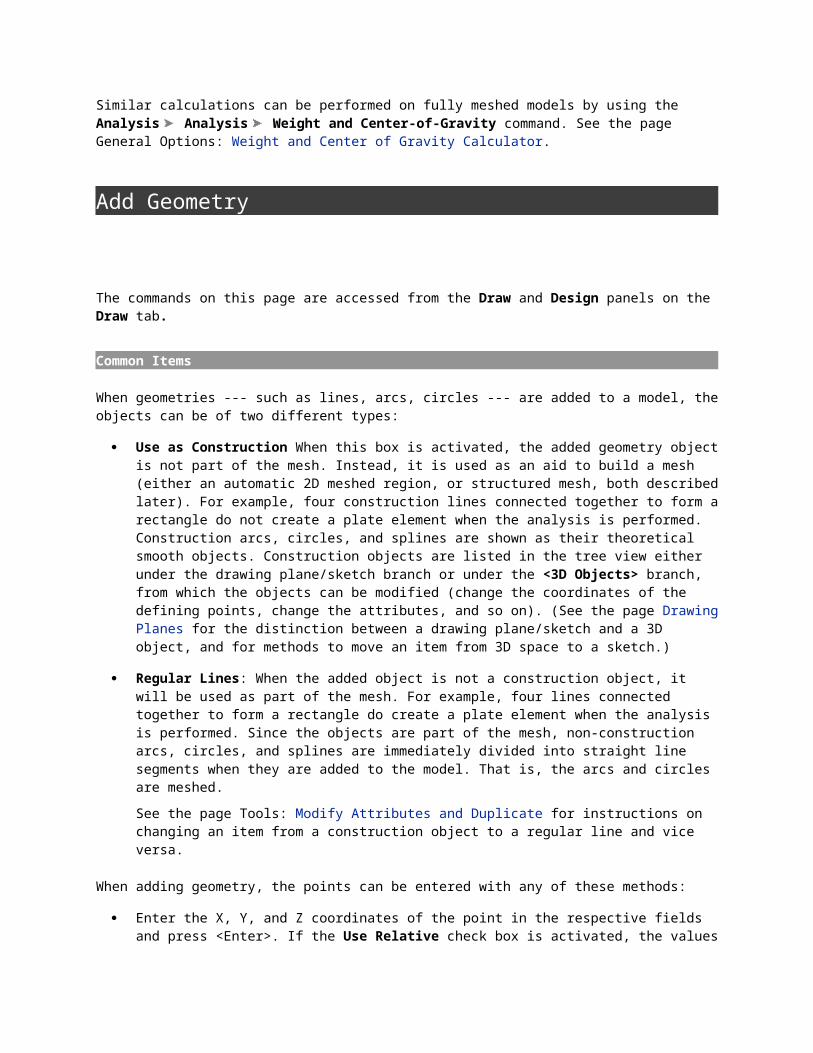
A': This point is where point A will be moved, or the origin of the new plane.

B: Points A and B define a local axis for the original plane.

B': This point will be used to define a line with point A'. The original geometry will be moved and rotated so that the line from point A to point B will be made parallel to the line from point A' to point B'.

C: This point defines a plane (along with points A and B).

C': This point will be used to control the orientation of the geometry in the new location. It defines the new plane along with point A' and B'. The plane defined by A-B-C is co-planar with the plane defined by A'-B'-C'.

If you want line AB to be the same length as line A'B', activate the Scale check box.

(a) The red rectangle is to be moved so that point A corresponds with point A' on the blue line and rotated so that side AB aligns with the blue line. Relocate & Scale defines the six points.

(b) Imagine a right-handed coordinate system created by each set of three points.

(c) Plane AB-AC is moved and rotated to align with plane A'B'-A'C'.

(d) The final result. If the Scale check box had been activated, the base of the rectangle AB would have been the same length as the line A'B'.

Project To Plane


Draw Modify Project to Plane

If vertices are selected, right-click and choose Project.

The Project to Plane command will move vertices to the indicated plane parallel to the global axis. The lines attached to the vertices will be stretched.

A possible use of this method would be to move all of the vertices of an imported wireframe to the X=0 plane so that 2D elements can be used.

Select the vertices that you want to move.

Select the command.

Select the radio button for the coordinate that you want to change. Type the value that you want to set for that coordinate for the selected nodes.

Press the OK button to perform the move.

Set From Point

Activating the command: Draw Draw Set From Point

The geometry construction objects, such as adding lines and circles, or creating 4 point rectangular meshes, require the input of coordinates. These coordinates can either be entered in absolute coordinates - measured from the origin (0,0,0) --- or relative to the last point entered --- DX, DY, and DZ. To change where the last point is measured from, use the Draw Draw Set From Point command. Selecting this command will give the Set From Point dialog and show the coordinate of the current 'From' point in the Status Bar. Use one of these methods to create a new from point:

Click any vertex in the model to set the current 'From' point to the coordinate of the vertex.

If the Use Relative check box is not activated, the ID of an existing vertex can be entered in the ID field. This will load the vertex's coordinates into the X, Y, Z fields. Press the <Enter> key to set the 'From' point.

If the Use Relative check box is not activated, enter an absolute coordinate in the X:, Y:, Z: fields and press the <Enter> key. If the Use Relative check box is activated (checked), then enter a relative offset from the current 'From' point for the new 'From' point in the DX:, DY:, DZ: fields and press the <Enter> key.

Inquire

The commands on this page are accessed from Tools tab Inquire panel in the FEA Editor.

Number of Objects in a Model

Count Total Objects: Selecting this command will launch a dialog that will display how many objects are in the current model.

Number of Objects in the Current Selection Set

If multiple lines, multiple construction objects, and so on are selected, right-click and choose Inquire to get a tooltip with the number of items selected.

Properties of an Object

To determine the properties of an object, whether a part, surface, line, and so on, select the object, right-click, and choose Inquire. The types of properties shown will depend on the selection. For example, the inquiry for lines will give the length, coordinates of the ends, and the part, surface, and layer numbers of the line. TipThe tooltip appears briefly when the cursor is held over an object regardless of whether it is selected or not. Selecting the object and using the right-click Inquire command will display the tooltip until the mouse is clicked somewhere else.

Lengths of the Shortest and Longest Lines in a Model

Minimum and Maximum Length: Selecting this command launches a dialog box that displays the length of the longest line in the model and the length of the shortest line in the model. The relevant lines are also selected in the display area.

Knowing the longest line can help locate overlapping lines that may exist from poor meshing techniques. Knowing the shortest line is useful when setting a search tolerance before doing a global snap; the tolerance should be less than the shortest line.

Measure Distances

There are multiple ways to measure distances in the FEA Editor:

Use Tools Inquire Measure to get a measuring dialog box. When in line selection mode (Selection Select Lines or Construction Objects), clicking on an object will give the coordinates of the endpoints and the DX, DY, DZ for the object in the Length of last selection section. When in vertex selection mode (Selection Select Vertices), clicking on a node will snap a rubber band to that node. Click another node to get the distance to the node, and so on. For each measurement made, the total is given in the Cumulative length section. Use the Reset button to clear the cumulative measurement.

If two vertices are selected (Selection Select Vertices), right-click and choose Inquire. A tooltip will appear with the distance between the vertices.

TipUse the Options Setup dialog and set the Decimal under Inquire to control the precision of the numbers shown in the tooltip.

Determine the Angle Between 3 Vertices:

Selected Vertices Angle: Selecting this command will launch a dialog box that will display the angle between the last three points selected. Alternatively, select three vertices, right-click and choose Inquire.

Determine the Angle Between Two Lines:

Selected Lines Angle: Selecting this command will launch a dialog that will display the angle between the last two selected lines. The lines need to share a common vertex.

Utilities

The commands on this page are accessed from Draw tab Modify panel in the FEA Editor.

Automatic Corrections to Meshes:

In some situations, wide-spread modeling mistakes can be corrected by using the following commands. This generally occurs when a mesh is imported from a source not designed for FEA, such as importing a CAD drawing.

For example, lines may cross over each other without being intersected, so the end points are not connected. This situation does not form a valid mesh. (Use the Global Intersect command.) Or, the end points of lines may be close but not exactly connected together, so elements are not formed in this situation. (Use the Global Snap command with the search tolerance large enough to snap nodes together.)

Global Snap: This command will snap together all the points that are located within the tolerance specified through the Set Search Tolerance command. This operation will be performed on the entire model. Note

The FEA Editor keeps duplicate vertices at the boundaries between adjacent parts, similar to how duplicate lines are required at the boundaries between parts. Consequently, the Global Snap command always reports that vertices between adjacent parts are combined, regardless of how many times the command is used. In most cases, combining these duplicate vertices will not change the model --- unless there are real gaps between the endpoints of the lines. Also, every line has a midside node which can be snapped to adjacent lines.

If the parts are bonded, then the duplicate vertices will be collapsed to one node number when a Check Model or analysis is performed.

Delete Short: This command will delete all lines in the model that are shorter than the distance specified through the Set Search Tolerance command.

Delete Unconnected: This command will delete all lines that are not connected to another line at either end.

Global Intersect: This command will intersect all of the lines in the model with the other lines in the model.

Remove Duplicate Lines: This command will remove duplicate lines in the same part. These lines are often created during some of the structured mesh routines.

Set Search Tolerance: This command will allow you to specify the CAD Preparation Tolerance. This tolerance will be used for many of the commands in this menu. This value is a length. NoteThe search tolerance is also used to determine whether two end points are the same or distinct. The tolerance is used when the FEA Editor prevents identical lines from being

created, where identical means that the lines have the same end points and are on the same part number. This rule has an effect when adding geometry, copying, meshing, and so on.

Modify Autodesk Inventor Parameters

When you work with an Autodesk Inventor model within Autodesk Simulation, you can access the Inventor parameters to change the model dimensions. You can change parameter values, update your model, and export the changes to the source Inventor model.

To access Inventor parameters, click Mesh CAD Additions Inventor Parameters. Most parameters display under the feature and the Model Parameters; use either one to change the parameter.

Parameter Name The name of the parameter. (Read-only)

Unit

For a numeric parameter, the units of measurement for the parameter. Currently, the units and values are based on the Model Units; they do not change with the Display Units. (Read-only)

Equation The equation that corresponds to the parameter value and unit. (Read-only)

Value

The value of the parameter. Modify values and press Enter. Changed values are shown in bold font. Currently, equations, text, and true/false parameters cannot be changed.

Inventor Equation The equation as imported from Inventor. (Read-only)

Inventor Value The value as imported from Inventor. (Read-only)

Update

Click to update the Autodesk Simulation model with the new parameter values. Note that some features may appear or disappear depending on any errors that occur while the Autodesk Simulation model is updated. The Inventor model is not changed by using Update.

Export

Click to export parameter values to the source Inventor model. In the Export Parameters dialog box, choose to export parameters for a Single Part or the Entire Assembly. Click OK to export. The Export also updates the Autodesk Simulation model if the changes have not been updated.

Meshing Hand-built Models

In addition to importing a CAD solid model and meshing, there are numerous methods of creating meshes by hand. Some examples include the following:

Create construction objects that form the edges of a region, and then use structured meshing to create a mesh in each region. By meshing multiple regions, the complete model can be constructed.

If the mesh is composed of planar geometry (plates or 2D elements, or if the surface of the solid is flat), then create a sketch of each plane. As long as the sketch encloses a complete region, the regions can be meshed with the 2D mesher.

For solid models, the interior mesh can be created automatically if the surface mesh that encloses the region is created. Select the part, right-click, and choose CAD Mesh Options Create Solid Mesh. (See the page Meshing Overview: Meshing CAD Solid Models, Model Mesh Settings: Solid for details on the solid mesh generation. Although this situation is not a CAD solid model, the solid mesh generation is the same.)

Meshes can be created in some situations by extruding a mesh. A plate element model can be created by drawing the edge of the plate, dividing the line into multiple segments, and extruding the segments to create an area. A solid mesh can be created by starting with a mesh of the face and extruding the area mesh to create a volume mesh. (See the page Meshing Overview: Creating and Editing Geometry in the FEA Editor: Tools: Move, Rotate, Scale, or Copy for details.)

For simple line geometry, such as beam and truss models, the elements can be drawn directly as lines. For other meshes, small regions can be created, or distorted areas repaired, by drawing lines. (See the page Meshing Overview: Creating and Editing Geometry in the FEA Editor: Adding Geometry for details.)

This section will concentrate on the first two methods. See the following pages.

Structured Meshes

2D Mesh Generation

Keep in mind that the technique used to create the mesh is not as important as the final result. As long as the mesh is representative of the part and gives accurate results, how it was created does not matter. For example, three different engineers might create a plate element mesh of a pipe in three different fashions:

Engineer A draws two construction circles that represent the ends of the pipe. After dividing the circles into two arcs, the Mesh Structured Mesh Between 2 Objects command is used to create the mesh between the arcs, thereby creating a mesh of the surface of the pipe.

Engineer B draws one construction circle that represents the end of the pipe. After dividing the circle into two arcs, the Mesh Structured Mesh Divide 1 Object command is used to divide the arcs into mesh lines of the perimeter. These mesh lines are then extruded (Draw Pattern Move or Copy) along the length to create a mesh of the surface of the pipe.

Engineer C draws one line that represents the length of the pipe. The line is divided into mesh lines, and these mesh lines are revolved (Draw Pattern Rotate or Copy) around the centerline to create a mesh of the surface of the pipe.

Topics in this section Structured Meshes 2D Mesh Generation

Structured Meshes

Use the commands on the Mesh tab Structured Mesh panel to create structured meshes - a mesh with a regular pattern. The basic steps are as follows:

1. If using one of the object meshes to mesh between objects (such as lines, arcs, splines), then create that geometry using construction objects. That is, activate the check box Use as Construction when drawing the item.

2. Issue the command to create the mesh. A dialog will appear.

3. Specify the attributes of the mesh in the Attributes section of the dialog. Attributes consist of the part, surface, and layer number of the lines that make the mesh.

4. Specify the number of divisions for the mesh in the Divisions section of the dialog. The divisions control the number of elements along the sides of the mesh. Also, whether the size of the elements are uniform or include some type of progression is specified from the Divisions section.

5. Specify the control points for the mesh. When creating a mesh between points, vertices or coordinates are used to specify the corners of the mesh. When creating a mesh with objects, click existing construction objects. (Be sure that the Selection Select Construction Objects is set, which it should be by default.)

Generally, the parameters on the dialog are specified left to right: attributes first, then divisions for each edge, then specifying the points or objects that define the mesh. But these parameters can be entered in any order prior to clicking the Apply button.

Specify the Number of Divisions for Unevenly Spaced Meshes

The Divisions section of the mesh dialogs includes the controls for the number of divisions (or elements) created along the respective edge of each mesh. The designations AB, AA', and so forth, change for the respective type of mesh. Naturally, the number of divisions AB is the number between points A and B, and so on.

By default, the divisions in these meshes will be evenly spaced along each edge or object. This can be changed by pressing the button next to each division. In the dialog that will appear, you can choose between the Constant, Arithmetic and Geometric radio buttons. The Constant radio button will create the default mesh that is evenly spaced. If the Arithmetic radio button is selected, the length of the lines from the first point to the second point will increase by a constant value. For example, if the first segment is 1.0 unit, the second may be 1.5, the third 2.0 and so on. Each segment will be 0.5 units larger than the last. If the Geometric radio button is selected, the ratio of adjacent segments will be a constant factor, with the length of each element increasing from the first point toward the second point. For example, if the first segment is 1.0 unit, the second may be 1.5, the third 2.25 and so on, the length of each segment being 1.5 times the length of the previous segment.

Arithmetic spacing: total length = h + (h+r) + (h+2r) + + (h + (n-1)r) = n[2h + (n-1)r]/2

Geometric spacing: total length = h + hr + hr 2 + + hr n-1 = h(1-r n )/(1-r)

where h is the shortest length, n is the number of divisions, and r is the increment or ratio between segments.

If either the Arithmetic or Geometric radio button is selected, you will be able to choose a controlling factor in the Control section. If the Short Length radio button is selected, you must specify the length of the first segment in the adjacent field (h). The constant increment or ratio will be calculated using this value and the total length of the edge. If the Ratio radio button is selected, you must specify the ratio of the longest segment to the shortest segment in the adjacent field. The first segment length and constant increment or ratio will be calculated using this value and the total length of the edge. If the Adjacent radio button is selected, you must specify the ratio of adjacent segments in the adjacent field (r). The first segment length will be calculated using this value and the total length of the edge.

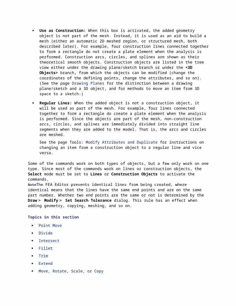
Figure 1: 4 Point Mesh with Nonuniform Spacing

Side AB has 4 divisions with a geometric spacing.

Side BC has 6 divisions with an arithmetic spacing.

The shortest segment is always near point A and expands away from A.

Structured Meshes Between Points in a Model

3 Point Triangular,

4 Point Rectangular and

8 Point 3D:

These three commands will create structured meshes between points on a model. You will need to specify the points of the mesh in a specific order (either clockwise or counterclockwise) for each mesh command. The points can be specified by clicking on a vertex on the model or a sketch (a padlock icon will appear when the cursor is over a vertex), by specify the coordinates of each point, by entering an existing vertex number in the ID box, or any combination of these.

For each of the command, follow the prompts to specify the points. The shapes are as follows:

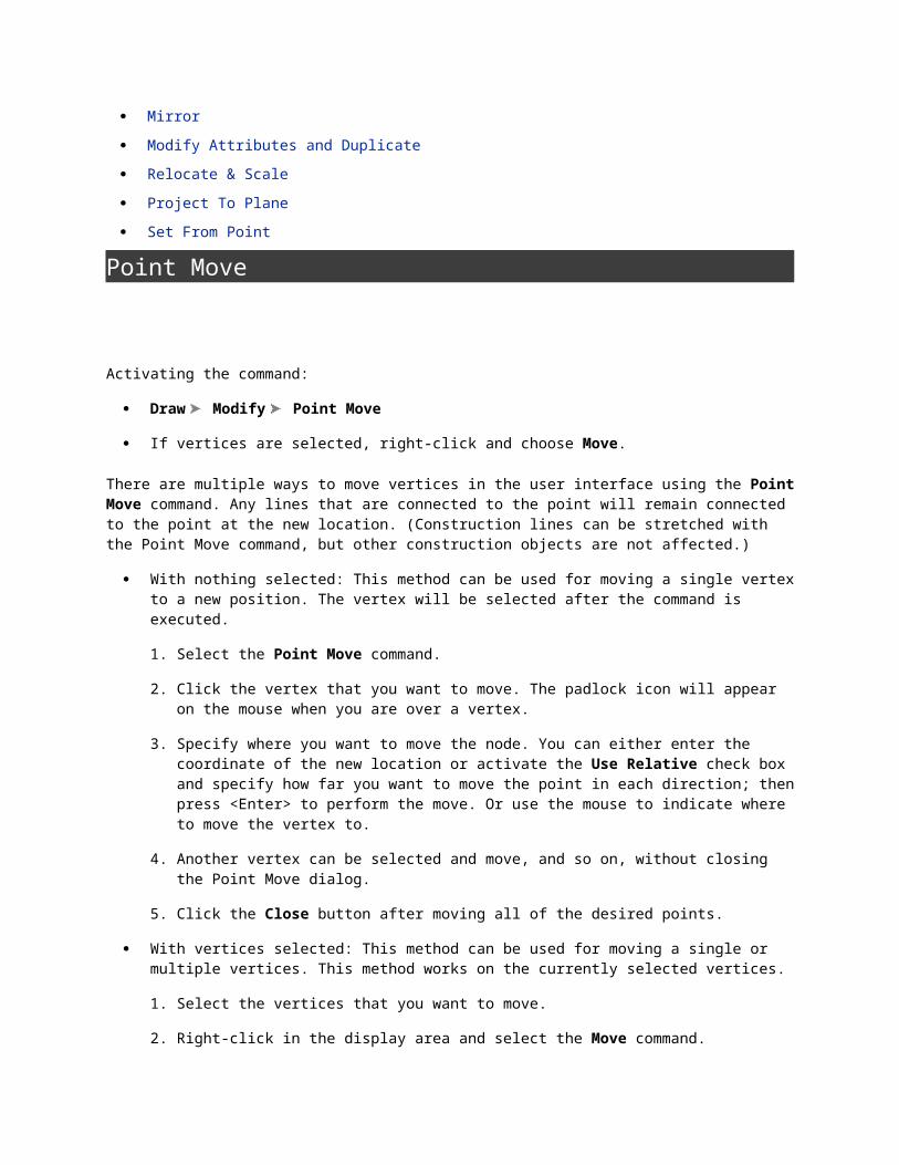
3 Point Triangular: For this mesh, you will define three points: A, B and C. The first point will be point A, the second will be Point B and the third will be point C. Triangular elements are created at point A; the rest of the mesh is quadrilateral elements.

4 Point Rectangular: For this mesh, you will define four points: A, B, C and D. The first point will be point A, the second will be Point B, the third will be point C and the fourth will be point D. These points must be selected in either a clockwise or counterclockwise sequence.

8 Point 3D: For this mesh, you will define eight points: A, B, C, D, A', B', C' and D'. The first point will be point A, the second will be Point B, the third will be point C and the fourth will be point D. The fifth through eighth points will follow the same order from A' to D'. These points must be selected so that a 4 point rectangular mesh will be created between points A, B, C and D and another 4 point rectangular mesh will be created between points A', B', C' and D'. The two meshes will be connected together, A to A', B to B', C to C', and D to D'.

Once the attributes, points and divisions are specified, you can press the Apply button to create the mesh.

Structured Meshes Between Construction Objects:

Divide One Object, Between 2 Objects, 4 Object 3D

These commands create structured meshes between construction objects. You specify the objects of the mesh in a specific order for each mesh command, as described below. The objects can be specified by clicking a construction object on the model.

The Geometry Mesh Divide 1 Object command gives results that are similar to the Draw Modify Divide command but has the following differences in the execution:

1. Divide One Object works on a construction object to create the lines in the FEA Editor. Consequently, the original construction object remains so that it can be used for other operations. (The Divide command splits the original object.)

2. Divide One Object can create nonuniform spacing. (The Divide command splits the object into uniform segments.)

3. Divide One Object is associative; the parameters for the mesh can be modified later (see How to Modify The Mesh below).

Divide One Object: For this mesh, you will select one construction object. The end point nearest to where you selected it will be point A.

Between 2 Objects: For this mesh, you will select two construction objects. The first object will be object AA'; the end point nearest to where you selected it will be point A. The second object will be object BB'; the end point nearest to where you selected it will be point B.

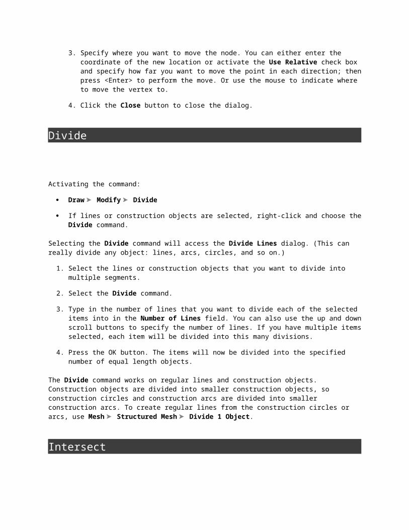
4 Object 3D: For this mesh, you will select four construction objects. The first object will be object AA'; the end point nearest to where you selected it will be point A. The second object will be object BB; the end point nearest to where you selected it will be point B. The third object will be object CC'; the end point nearest to where you selected it will be point C. The fourth object will be object DD'. The end point nearest to where you selected it will be point D. See the following figure for connectivity.

Once the attributes, objects and divisions are specified, you can press the Apply button to create the mesh.

Edit Structured Meshes

When a structured mesh is created, an entry appears in the tree view under the Meshes branch. To modify an existing mesh, select the entry in the tree, right-click and choose Edit. All parameters related to the mesh can be changed. When the Apply button is clicked, the mesh is revised. Also, any operation done to the mesh that appears in the Meshes branch will be updated also. For example,

1. Create a 4 point mesh (Mesh Structured Mesh 4 Point Rectangular) of any size. Use 4 divisions on each side.

2. Select the 4 point mesh entry in the Meshes branch of the tree view, right-click, and choose Move or Copy.

3. Activate the Copy and Join check boxes to make an extrusion. Set the number of copies to be 3 and the direction to be perpendicular to the plane of the mesh. Set the total distance to approximately the size of the mesh. Click the OK button to perform the copy operation.

4. Select the original 4 point mesh entry in the Meshes branch of the tree view again. Right-click and choose Edit.

5. Change the number of divisions to 6 for each side.

6. When the Apply button is clicked, the original mesh and the copy/extrusion are updated. (If the lines of the mesh had been selected and copied instead of selecting the mesh, changing the mesh would have had no affect on the extruded lines.)

Tip

To change the points or objects associated with a mesh, use the ESC key to back through the selected items. This can be used while creating the original mesh or while modifying an existing mesh.

For example, when the mesh is modified in the above example (step 4), click the Escape key after the Point Mesh Setup dialog appears. Point D is removed, so now you can select a new point D. The ESC key can be used to remove all of the selected points or objects, allowing them to be respecified.

2D Mesh Generation

The 2D mesh generator is an advanced tool for automatic mesh generation of any enclosed region drawn in any plane. This generator allows you to automatically mesh fairly complicated regions with one simple command. The 2D mesh generator offers mesh refinement options which allow you to quickly and easily refine your mesh by putting more elements at critical points in your design.

The general process is as follows:

1. Create a sketch of the wire frame (or outline) of each part. Each wire frame must be

composed of construction objects (not regular lines),

must form a continuous, enclosed region with any number of internal holes, and

each region within a given plane must be drawn on a different part. (See Meshing Overview: Creating and Modifying Geometry in the FEA Editor: Drawing Planes for more information.)

Optionally, set the surface number of the construction objects to aid with applying multiple loads and boundary conditions to the part. (By default, each edge of the mesh is on a unique surface number, but the mesher has an option to assign the surface number of each edge based on the construction object's surface number.)

TipTo have a node appear at a specific location on the wire frame, split the wire frame at that location. The 2D mesh generator creates nodes at each endpoint of the construction objects. For example, to place a node at the 30 degree position on the perimeter of a hole, draw a temporary construction line that intersects the circle at that position, and then use Draw Modify Intersect to split the circle.

2. Specify edge divisions and refinement points if desired. See Specifying Edge Divisions and Refinement Points for more information.

3. Once all of the sketches are complete, you can generate the 2D mesh by selecting the drawing plane under each part headings in the tree view, right-clicking, then choosing the Create 2D Mesh command. The 2D Mesh Generation screen will appear. All parts on a given plane should be meshed together to assure that the meshes match between the parts. Different planes are meshed separately. For information on the options in this screen, see Generating the 2D Mesh.

TipInstead of selecting multiple sketches individually, you can right-click the drawing plane entry under the Planes heading in the tree view and choose Select all Sketches. This highlights each sketch under the parts in the tree view associated with the drawing plane. Deselect sketches that are not to be meshed.

NoteAlthough the 2D mesher can mesh a region in any drawing plane, if used to create 2D elements, the sketch must be in the YZ plane at X=0.

To use the 2D mesher, the construction objects must be drawn in a sketch on a drawing plane; they cannot be 3D objects which are a separate branch of the tree view. 3D objects cannot be used in the 2D mesher even if they lie in the same plane as other sketch objects. Click the sketch in the tree view to see the objects belonging to the sketch. NoteSee the page Meshing Overview: Creating and Modifying Geometry in the FEA Editor: Drawing Planes for instructions on moving the 3D objects to a drawing plane/sketch.

Using Multiple Parts and Planes:

The 2D mesh generator will mesh one plane at a time. When working with assemblies consisting of multiple parts within the plane, it is important to remember that each part must consist of a single enclosed area. Figure 1 below shows some valid and invalid regions.

(a) Valid Region - with three holes (b) Invalid Region - break in outer boundary

(c) Invalid Region - break in inner boundary

(d) Invalid Region - intersecting boundaries

(e) Invalid Region - touching boundaries (f) Invalid Region - touching boundaries

Figure 1: Example Sketches for Purposes of 2D Mesh Generation

Imagine that the three holes in Figure 1(a) are to be filled with another material (and for discussion, assume that everything shown in the figure is drawn on part 1). A rectangle drawn on part 2 and over top of the rectangular hole in part 1 would fill the rectangular hole. A circle would be drawn on part 3 to fill the circular hole, and a semi-circle would be drawn on part 4 to fill the semi-circular hole.

Another important situation for some analysis types is shown in Figure 2.

For analysis types that do not support smart bonding, when two parts are meshed together, each part must have a matching segment for the mesh to match at the interface. The top edge of the large rectangle must be drawn using three lines to ensure that the mesh along the shared edge matches up correctly.

For analysis types that do support smart bonding, the parts do not need to have matching segments in the sketch. See the page Meshing Overview: Creating Contact Pairs: Types of Contact for the analysis types that support smart bonding.

Figure 2: Matching Between Parts without using smart bonding

Topics in this section Specify Edge Divisions and Refinement Points Generate 2D Meshes

Specify Edge Divisions and Refinement Points

Before generating the 2D mesh, there are two items that can be specified to control the mesh size in specified areas: Edge Divisions and Refinement Points.

Edge Divisions

In some situations, you may want to control how many elements are created along a particular edge. You can do this by selecting the construction object and right-clicking. Select the 2D Mesh Divisions command. The Sketch Entity Mesh Division dialog will appear. Activate the Specify division check box and type the number of divisions that you want to be made along the selected edge. The number of divisions can be fewer than what the mesher would try to create, but a better mesh will be created if the number of divisions is approximately the same or more than the number of divisions that the mesher will create (based on the mesh size).

2D mesh generation matches the mesh between different parts only if the parts are meshed simultaneously. Parts meshed separately in different planes normally do not have matched meshes.

Refinement Points

Refinement points specify a region in which the 2D mesh generation will create a finer mesh. The input is identical to the refinement point dialog described for CAD solid models. Refer to the page Meshing Overview: Meshing CAD Solid Models: Refinement Points for details.

Generate 2D Meshes

Once all of the sketches are complete, you can generate the 2D mesh by selecting the drawing plane under each part headings in the tree view, right-clicking, then choosing the Create 2D Mesh command. The 2D Mesh Generation screen displays. TipTo select multiple sketches, right-click the drawing plane entry under the Planes heading in the tree view and choose Select all Sketches. Under the parts, each sketch associated with the drawing plane is highlighted. Deselect sketches that will not be meshed.

All parts on a given plane should be meshed together to assure that the meshes match between the parts when required. Different planes are meshed separately.

2D mesh generation matches the mesh between different parts only if the parts are meshed simultaneously. Parts meshed separately in different planes normally do not have the meshes matched. NoteSee Specifying Edge Divisions and Refinement Points to use Edge Divisions to help match the mesh in different planes.

When you select a plane heading in the tree view and select the Generate 2D Mesh command, the 2D Mesh Generation dialog will appear. The dialog includes the following features.

Element Shape

Quadrilateral: Selecting this option instructs the mesher to mesh the region using only quadrilateral elements. Note that this option always splits each segment into a minimum of two divisions. When very short segments exist, some distorted elements may occur in the area. Using a mixed mesh or adding refinement points (Specifying Edge Divisions and Refinement Points) may be helpful.

Triangular: Selecting this option instructs the mesher to mesh the region using triangular elements.

Mixed: Selecting this option instructs the mesher to mesh the region using both quadrilaterals and triangles. This option may be useful when the wireframe contains very short segments or thin parts. The mixed mesh does not require each segment to be split into a minimum of two elements, and this results in a more uniform mesh around these short segments

Surface Number

The option Use Surface Number of Construction Object controls the surface number of the lines generated in the mesh.

When not activated (unchecked), the surface of each edge of the mesh is placed on a unique number. (Technically, the surface number of each edge is equal to the construction object's number - as shown in the tree view --- plus 1. Thus, no two parts will have the same surface number around the perimeter.)

When activated (checked), the surface number of each edge of the mesh is placed on the same surface number as the construction object's surface number. This is convenient when multiple edges are destined for the same load. For example, imagine a tube sheet in a heat exchanger with 50 holes. To apply a boundary condition around the perimeter of these 50 holes (to simulate the connection to the tubes), draw each hole in the sketch on the same surface number. After meshing, select this one surface to apply the boundary condition.

In both cases, the surface number of the interior lines is 1. Thus, do not use surface number 1 for a construction object that needs a surface-based load or boundary condition when the Use Surface Number of Construction Object option is used. NoteConstruction object color is controlled by the option Options Sketching Color of construction objects follows View: Color By. The color is either black or follows the part, surface, layer number of the object which is set by the View Appearance Color By drop-down menu.

The surface number of the construction object can be set while the object is drawn. After it is drawn, it can be changed by selecting the object (Selection Select Construction Objects), right-clicking, and choosing Edit or Edit Attributes.

Global Element Size

Mesh Density This option is roughly the number of elements in a rectangle completely enclosing the geometry. Holes, arcs and refinement points will affect the actual number of elements generated. If this item is active then the non-refined mesh size is set based on the number of elements that will fit in a rectangle which encloses the model. The actual number of created elements can be larger or smaller than the specified density. If the model does not fill the entire enclosing rectangle, the number of created elements can be much less than the specified density. Similarly, if the model contains refinement points, the model can have many more elements than the specified density. The default value of 400 should be a good first approximation for most models. After the first mesh, you can add refinement points to selectively refine the necessary regions.

Mesh Size If this radio button is selected then the non-refined mesh size is specified by the mesh size value. Elements near refinement points will have edges smaller than this value. Also, the size of internal elements can vary from this value because of smoothing and the appropriate use of existing nodes. This parameter is an alternative to setting the desired size of the non-refined elements by specifying the density.

Advanced

Angle: Specify the minimum angle for the division of arcs, splines and NURB curves. Curved edges are divided based on the designated angle if it will result in smaller elements than the standard mesh size. This provides higher mesh densities at sharp bends where stress concentrations are likely to occur. The region inside the circle (or the circle that corresponds to the extended arc) is meshed with the same mesh density as the circle itself. A transition region around the curve allows the mesh to increase geometrically from the edge of the curve to the standard non-refined mesh.

Geometric Ratio: The geometric ratio defines the approximate size ratio of adjacent elements. Selecting this command allows you to change the geometric expansion ratio used by the mesher. This ratio is used to determine how quickly a refined mesh will make the transition to the non-refined density. A value close to 1 results in slow transitions from higher to lower density regions. As the value increases, this transition occurs faster.

Close Factor: This value times the local mesh size determines the range within which the 2D mesh generator searches for close nodes. It uses this to determine both if it should connect to a close node and to look for crossing lines due to close nodes. Larger values make the algorithm more robust, but can lead to elements with higher aspect ratios (up to the close factor). The default value is 4. A typical range is from 2.0 to 10.0.

Refine Factor: The Refine Factor is used to quickly change the mesh size --- especially the refinement points --- without needing to edit each item. The global mesh size and refinement point factors (mesh-size based) are divided by this input. Only whole numbers are acceptable.

Tolerance

Automatic: The auto-tolerance value defines the maximum distance between two points that are considered the same.

Use: Selecting this command allows you to change the tolerance used by the automatic mesher to determine if the end points of boundary items represent the same point. Usually, this should be set at Automatic and the meshing algorithm will

calculate an appropriate value. If the 2D mesh generator reports breaks in the boundary, you can try adjusting the tolerance to allow the 2D mesh generator to be less critical.

Generate the 2D Mesh

Click the Apply button to generate the mesh.

If the mesher detects an error --- such as a break in the sketch outline or overlapping lines on the same part number- it will report that the wireframe does not enclose a single area. It marks the problem area on the model with red triangles. See Figure 1. The red triangles will be removed after correcting the sketch and successfully generating the 2D mesh. (If multiple parts have problems, the mesher will identify the problem in the first part. After fixing it and trying to generate the mesh, the mesher will detect and display the problem in the next part, and so on.) See the introduction for examples of proper and improper sketches for 2D meshing.

Figure 1: Two Part Sketch That Fails the 2D Meshing

The upper part is missing a line segment on the right side.

The red triangles mark the problem areas in the wireframe.

Surface Mesh Enhancing

The surface mesh enhancement process provides automatic surface mesh enhancement for any valid surface mesh (plate/shell models or surfaces of a solid model), one part at a time. It can make surface meshes more consistent, improve the shape of elements and reduce the overall mesh density. Two or three days worth of manually meshing plate/shell models, for example, can be performed with surface mesh enhancement in just minutes.

The surface mesh enhancement is important, because the surface is where high stress areas are usually located and where loads and constraints are applied. An improved surface is also important in the generation of a solid mesh. The solid mesh process creates bricks from the outside in and bases its construction on the exterior surface of a model. The more regular and consistent the surface and surface elements are, the more regular and consistent the brick mesh will be.

The surface mesh enhancement process will use any refinement points that have been defined. See the page Meshing Overview: Meshing CAD Solid Models: Refinement Points for details on refinement points.

The return file from the surface mesh enhancement contains the mesh generated by the mesher. It may also contain yellow Layer 3 lines. The Layer 3 lines occur whenever the surface mesh enhancement divides a quadrilateral into a triangle. This is done to avoid warped elements.

Surface mesh enhancement works from the existing mesh. The new mesh is based on the surface of the existing mesh. If a model has a coarse mesh such that a hole is 10 sided, enhancing the mesh and specifying a smaller mesh size results in a finely meshed 10-sided hole; the enhancement does not know that the hole is theoretically round --- even when enhancing a CAD model. For this reason, the normal procedure when working with curved surfaces is to start with a fine mesh and use the mesh enhancement to generate either a larger mesh size or similar mesh size. TipWhen working with a CAD solid model assembly, the normal Mesh Mesh Generate 3D Mesh command offers many advantages over the surface mesh enhancement. Use the surface mesh enhancement only if the desired mesh cannot be obtained from the regular surface mesher.

Perform a Surface Mesh Enhancement:

1. If not already set, set the Element Type for the part to be enhanced.

2. Select Mesh Mesh Enhance Surface Mesh. The Surface Mesh Enhancement dialog will appear.

3. Set the following settings as desired:

Part #: Enter the number of the part that you want to perform the enhancement on.

NoteDo not try to enhance a part that is already solid meshed. The element type can be set to brick, but the part being enhanced must be a surface mesh only. When working with a CAD model, determine if a part is solid meshed by checking the Draw Design Layer Control lines on layer 0 are the solid mesh. Use the View Appearance Internal Mesh to see the interior mesh created by the Solid Mesh Engine.

Absolute Mesh Value: This will be the approximate size of the elements. The size can be entered in the field to the left or can be altered by moving the slider. Note that the default value shown for the mesh size is not necessarily related to the current mesh size.

Percentage of Default: This will determine the approximate size of the elements as the percentage. The percentage can be entered in the field to the left or can be altered by moving the slider. The default mesh size is one sixth of the cube root of the volume.

Options button: For more options, press the Options button. (See the page Options Button below.)

NoteSet the Options Feature Layer to 15 before enhancing the mesh as only one part at a time, of a CAD assembly, can be enhanced. Matching lines, between the CAD parts, will automatically be placed be on Layer 15 by the CAD surface mesher (Mesh Mesh Generate 3D Mesh).

4. Press the Mesh button to enhance the surface mesh. The status box will provide some basic feedback on the progress, or use the Details >> button to see more in-depth feedback from the mesh enhancer.

5. The enhanced mesh is not displayed until the dialog is closed. Press the Done button to exit the screen.

6. After closing the dialog and reviewing the enhanced mesh, you can return to the previous mesh by opening the Surface Mesh Enhancement dialog and clicking the Undo button. Only one undo can be performed.

The surface mesh enhancement process defaults to accepting a watertight-surface model; that is, a mesh that fully encloses a volume. Such meshes are typically filled with brick elements in a later step using the Solid Mesh command. In addition to a watertight mesh, the model cannot have any internal partitions. Internal partitions are inner surfaces. TipSurface mesh enhancement can also be used on plate models and other surface meshes that do not form a water tight mesh. Set the Open Plate Model option as described in Options Button: Mesh Shape/Quality below. NoteIf you get an error during a surface mesh enhancement, see the page Correcting Topological Errors.

Topics in this section Options Button Correcting Topological Errors

Options Button

The options dialog is broken down into three different tabs: Mesh Shape/Quality, Features/Refinement and Advanced. Click the link to the tab that you need more information about.

Topics in this section Mesh Shape and Quality Features - Refinement Advanced

Mesh Shape and Quality

Surface Mesh Enhancement Options: Mesh Shape/Quality tab

Meshing Retries

This section allows you to control the parameters involving the retry operation that occurs when a mesh cannot be enhanced with the current parameters.

Retry Number: The value in this field is the number of times that the enhancer will retry the enhancement.

Retry Fraction: The value in this field will multiply the mesh size to calculate the new (smaller) mesh size that will be used on the next retry.

Mesh Type

The Mesh Type pull-down has options to generate a quadrilateral or triangular mesh.

Feature Controls

The surface mesh enhancer will take the existing mesh and put a new surface mesh on the model. The way the mesher finds the outline of the model is by using feature lines. Feature lines define the boundaries of the volume that the model encompasses. The position of feature lines will stay in the model when a new mesh is created but can be divided into smaller lines or made into larger lines. In other words, a feature line is a key edge of the model. A feature cannot change positions without changing the outline of the part. But the size of the elements along the feature can bet bigger or smaller.

There are two different ways to define feature lines in your model, the Feature Layer and the Feature Angle fields.

Feature Layer: You can specify lines in the mesh that you want the surface mesh enhancer to maintain. To specify a feature line, select the lines (Selection Select Lines) change the layer number to a specific layer number (Draw Modify Attributes). Then, set the Feature Layer to that same number. When you run the surface mesh enhancer, the feature will be maintained and the mesher will not mesh across this feature. NoteLayers 14 and 15 are automatically treated as feature layers. If you do not want to preserve these lines, change the layer numbers. (Layers 14 and 15 are created in CAD

meshes and represent the feature lines of the CAD model and the lines that match between parts, respectively.)

Feature Angle: The feature angle (expressed in degrees) is a setting used to determine whether a line is or is not made into a feature line. Feature lines are generated from the intersection of two elements. The elements' normal directions are calculated, and their difference is called the out-of-plane angle. If the two elements generate an out-of-plane angle larger than the feature angle, the line created by the intersection of the two elements is made a feature line. If the out-of-plane angle generated by the two elements is smaller than the feature angle, the line generated by their intersection is not treated as a feature line.

In other words, if the angle between the planes of two adjacent elements is larger than the feature angle, then the common edge between the two elements becomes a feature line segment. The mesher will not mesh across feature line segments.

A small feature angle will result in more feature lines, a more detailed mesh and a larger model that will take longer to analyze. A larger feature angle will eliminate excess feature lines, help reduce the noise or erroneous lines that can accompany some imported models, and produce a smaller model that can be analyzed in less time.

Too many feature lines (angle is too small) can prevent the mesher from finding a suitable mesh. Too few feature lines (angle is too large) can round off large, sharp edges as they are meshed when they should be kept as features. A large feature angle can also cause gaps to appear along the features. If these gaps are small, they can reduce the mesh size necessary for the mesher to mesh the model. The mesher assumes that the feature angle will be smaller than 90 degrees so that it can trace curves along the surface.

Delete Feature Layer: This option is used to prevent edges from becoming features even if they normally would be considered features based on the feature angle. It can be used to improve the quality of the mesh. You can remove skewed feature lines that would force the mesher to create triangular and/or skewed elements. It is not designed to remove features defined by feature angles larger than 89 degrees. Consequently, it cannot be used to remove small holes from a model. Removal of unwanted features, like small holes, should be done in a CAD package before generating the surface mesh.

The default layer number for this option is layer number 10.

Open Plate Model: This option lets you specify whether or not the surface mesh is watertight. Checking this box means that the mesh is not watertight; that is, you are enhancing the mesh for a plate model.

Features Only: The surface mesh enhancer will not perform the mesh generation if you use this option. This option causes the surface mesher to generate a separate model named feature.fem. The lines in the feature.fem file represent the feature lines in the model (based on the feature angle).

The features only file can be used to check whether the feature angle has been specified correctly. Since the surface mesher does not mesh across feature lines, all the lines in feature.fem file would be in the final model if it were enhanced with the same settings. Examples

This section shows two models. The free-form model, shape, will be used to show what happens when the feature angle is too small. The more geometric model, tank, will be used to show what happens when the feature angle is too large. Both of these models can be meshed reasonably well using the default settings for feature angle and curve angle. Figures 1 and 2 show the meshes created with the default settings. The feature lines created in the feature.fem are acceptable. Figures 3 and 4 show the feature lines for the models.

Figure 1 The Shape Mesh with Default Settings

Figure 2 The Tank Mesh with Default Settings

Figure 3 Feature Lines for the Shape Model

Figure 4 Feature Lines for the Tank Model

If the feature angle is too small, then too many feature lines are generated. Some clusters of feature lines may seem to end in space and be difficult to mesh. You may need to decrease the mesh size until it is small enough to mesh the clusters. Figure 5 shows the result of setting the feature angle to 10 degrees. To remove the clusters, the mesh size is about 1/3 the default mesh size and about 10 times as many elements must be generated.

If the feature angle is too large, then feature lines will be missing and those features will be rounded off in the meshed model. Figure 6 shows the result of setting the feature angle to 70 degrees. Notice that the features defining the front edge are missing. Figure 7 shows the meshed version where the edges representing these features fluctuate based on element shape. To emphasize the effects of the feature angle and the curve angle, the mesh size for the tank model is set slightly larger than the mesh size for the default case.

Figure 5 The Shape Model with a Feature Angle of 10 Degrees

Figure 6 The Tank Model with a Feature Angle of 70 Degrees

Figure 7 The Tank Mesh with a Feature Angle of 70 Degrees

Features - Refinement

Mesh Mesh Enhance Surface Mesh Options Features/Refinement tab

General Parameters

Pre-Conditioning Factor: The pre-conditioning factor indicates how much larger than the element size you wish the surface mesh enhancer to search to connect close feature line nodes.

The default value is 1.2, indicating that the surface mesh enhancer will increase the mesh size by up to a factor of 1.2 to bridge the space between adjacent feature lines. A larger value (up to maybe 2) typically provides better results if your model has many areas with long, narrow features.

Quad Split Internal Node Angle: The surface quad internal node angle (in degrees) describes the maximum internal angle of any surface quad. If the internal angle of a quad is larger, the surface mesh enhancer divides the quad into two triangles.

Quad Split Fold (Warp) Angle: The quad warp angle (in degrees) describes the maximum out-of-plane angle between any two triangles that you can divide a quad element into. If the warp of a quad is larger, the surface mesh enhancer divides the quad into two triangles. The resultant line that comes from splitting the quad will be layer number 3.

Curve Angle: A feature segment is created along the common edge of two triangles that form an angle larger than the feature angle. These feature segments are connected together to form feature curves. Feature curves are initially divided where they intersect other feature curves or when the cumulative angle along the curve is larger than the curve angle. The resulting feature segments are then further divided based on the mesh size.

The curve angle (in degrees) describes how general curves are broken up. For example, if you have a circle with a size smaller than the mesh size, it may be divided into two lines. By specifying a curve angle, it ensures that the circle is divided at least every n degrees.

You will usually not need to change the curve angle. Its primary purpose is to decrease the mesh size along feature curves with a small radius of curvature.

The surface mesh enhancer tries to mesh feature curves so that the length along the feature curve between mesh points is as close as possible to the mesh size. Without the Curve Angle option, the surface mesh enhancer would mesh small holes (radius less than the mesh size) into too few segments.

The surface mesh enhancer divides feature curves whenever the angle between the starting segment and the current segment is larger than the curve angle. A feature curve is made up of simply connected feature segments. The edge between two triangles is a feature segment if the angle between the planar normals of the triangles is larger than the feature angle.

The curve angle prevents small holes, with circumferences less than the mesh size, from being reduced to a point which cannot be meshed.

The curve angle is used in the following way. The feature line segments are connected together to form feature curves. These feature curves are divided at nodes connected to more than two feature curves to create non-intersecting feature curves. The non-intersecting feature curves are then divided whenever the angle between the current segment and the initial segment of that curve is larger than the curve angle. The non-intersecting feature curves are meshed (broken into lines) based on the length of the curve, the mesh size and any mesh refinement close enough to affect the curve. Values larger than 90 degrees should not be used.

The image below gives a visual explanation of a curve angle. Whenever the angle between the starting segment and the current segment is larger than the curve angle, a new starting segment is created and the starting point of that segment becomes a node in the meshed model. If the points on a feature curve are named A, B, C, D, E, F and the angles between segments are:

AB to BC = 30

BC to CD = 28

CD to DE = 15

DE to EF = 20

Figure 1

Whenever the angle between the starting segment and the current segment is larger than the curve angle, a new starting segment is created and the starting point of that segment becomes a node in the meshed model. If the curve angle is 31 degrees, then the segments CD and EF will be new start segments and points A, C, E and F will remain nodes in the final model.

If the curve angle is 29 degrees, then segments BC and DE will be new start segments and points A, B, D, and F will remain nodes in the final model. If the curve angle is 31 degrees, then segments CD and EF will be new start segments and points A, C, E, and F will remain nodes in the final model. If the curve angle is 60 degrees, then segment DE will be new start segment and points A, D, and F will become nodes in the final model. Example

The curve angle affects how segment curves are divided. Figure 2 shows the feature lines obtained from setting the curve angle to 70 degrees. For this case, the four segments at the top of the cylinder are meshed as a pair of elements that are not connected to the rest of the model. See Figure 3.

Figure 2: Feature Lines for the Tank Model with a Curve Angle of 70 Degrees

Figure 3: The Tank Mesh with a Curve Angle of 70 Degrees

You can easily avoid this situation by using a smaller curve angle, using a smaller mesh size, or using a smaller feature angle. Figure 4 shows the same model meshed with half the mesh size. For this case, the mesh size is small enough so that the cylinder is divided into more than 4 segments.

Figure 5 shows the model meshed with a feature angle of 10 degrees. Feature curves are divided whenever they intersect other feature curves. Reducing the feature angle creates enough feature curves to resolve the top cylinder. Figure 6 shows the feature lines created with a feature angle of 10 degrees. Once all of the features are resolved with the feature angle, the feature curve does not affect the results.

Figures 5 and 6 are also identical to the results obtained by using a curve angle of 10 degrees. It is often useful to try small curve angles if you have problems getting the surface mesh enhancer to mesh a model. You can reduce the curve angle so that it is small enough to resolve the original feature segments. If the feature segments in the original model are similar in size and not close to a much larger feature line, then the surface mesh enhancer can generate a reasonable mesh. One of the results of choosing a small curve angle is that more elements are generated near curving boundaries.

Figure 4: The Tank Model Meshed with Half the Mesh Size

Figure 5: The Tank Mesh with a Feature Angle of 10 Degrees

Figure 6: Feature Lines for the Tank Model with a Feature Angle of 10 Degrees

Refinement Controls

Refine Near Short: This option will cause the surface mesh enhancer to refine the mesh along the short feature lines. This is useful if a short feature line is next to a longer feature line. It is especially useful if the model contains a few small holes.

Refine Near Gap: This option will cause the surface mesh enhancer to refine the mesh around small gaps between features. It is useful when the edge of one feature is much closer than the current mesh size to another feature.

Refinement Range: This specifies the transitional distance between the refined mesh size and the specified mesh size. The value in this field is a multiple of the mesh size. A small value will create fewer elements, but it may prevent the surface mesh enhancer from creating a proper transition region.

Once the surface mesh enhancer refines the model for a specific mesh size and refinement, the refinement range can be altered to improve the quality or decrease the number of elements. If the range is decreased, the transition region will be sharper and the number of elements will be reduced but poor quality elements may be produced in the transition region. If the range is increased, you will have a large transition region, a large number of elements, but lower chance of poor quality elements.

Clean Initial Triangles: This command will remove thin feature triangles that sometimes occur in stereolithography files. Feature triangles are triangles with two lines as feature edges. If the triangle height is greater than the input value, then the surface mesh enhancer will try to remove it.

If the specified value is negative, then the absolute value of the specified value times the mesh size is used as the feature clean height.

Clean Feature Lines: If three connected nodes are connected to 3 quads, 4 quads, and 3 quads respectively, the region can be topologically simplified by replacing all 10 quads with 4 quads. This usually makes a cleaner mesh and smoothing helps readjust the quad angles. If the outer boundary of this region is along features, then smoothing will not change any of the angles. For this case, we do not want to create quads with large internal angles. The 3-4-3 to 4 cleaning operation is not performed if a boundary angle between feature nodes is greater than the specified angle.

Advanced

Surface Mesh Enhancement Options: Advanced Tab

Tolerance

Internal Tolerance: This is the tolerance that the surface mesh enhancer will use to make elements between feature lines and to match up nodes.

Dangling Features

Delete Feature: If the surface mesh enhancer cannot extend the feature segment, it tries to remove dangling feature segments. It will remove a feature segment if the planar angle creating the segment is less than the Delete Feature field (in degrees).

Continue Feature: Dangling feature ends can cause meshing problems. The surface mesh enhancer first tries to extend the feature segment if it can find triangle edges that are within the Continue Feature field. If it cannot extend feature segments until they connect to another feature, it tries to remove dangling feature segments.

Features for Files

The following commands generate meshes in the Superdraw format. To view these files, use Open and set the Files of Type to Autodesk Simulation Superdraw III (*.esd).

Front.esd Only: This will create the front.esd file.

Input.esd Only: This will create the input.esd file. The input.esd is original surface mesh, converted to triangular elements, with the layer numbers changed to show which lines are feature lines and which ones are the normal mesh.

Correcting Topological Errors

If topological errors are found in the file, the surface mesh enhancer may display messages directing you to other files, such as:

****ERROR: Errors in input (Holes=Purple, Multiple=Red) See error. esd.

Also, a file named filename.erm may be created. The file contains the input file after all quads have been converted into triangles and any dangling and duplicate triangles have been removed. Dangling triangles have only one edge connected to the rest of the model.

Edges that are connected to only one triangle are shown as purple lines (layer 6). Edges that are connected to more than two triangles are shown as red lines (layer 2). To correct the topological problems, you can rename the filename.erm file to an extension .esd and use

Open command to view the file. (Set the Files of Type to Autodesk Simulation Superdraw III (*.esd).)

If the file is topologically correct but the surface mesh enhancer cannot complete the mesh, it generates a fatal error message and an filename.erm file. This file will include green lines for the elements that have been completed, blue lines showing the advancing front at which the surface mesh enhancer is currently creating elements and usually red lines that indicate the problem area.

Most of the surface mesh enhancer's meshing problems are a result of the mesh size being too large and are corrected by decreasing the mesh size. For these cases, there is not much value in looking at the filename.erm file as reducing the mesh size will correct the problem.

If reducing the mesh size does not correct the problem, you can examine the filename.erm files for several different mesh sizes. If the errors (red lines and/or points) occur in the same physical region, it may be useful to simplify the mesh in that region. Before trying to correct the mesh yourself, generate a feat.esd file and look at the region near the error (you can delete all but the red lines in the filename.erm file, save it under another name and then merge it over the feat.esd file to identify the problem region in the feat.esd file). If the problem region has skinny feature triangles, try increasing the -pc value to remove some of the feature triangles.

If the feat.esd file doesn't indicate the problem or if increasing the Clean Initial Triangles value doesn't correct the problem and you are an experienced hand-model builder, try to simplify the mesh in the region of the problem. There is difficulty in using a wire representation of a three-dimensional mesh on a two-dimensional screen. Careful use of the layer command can help in isolating the surface of interest. This is not always a fruitful approach because it is difficult to do and there is a good chance an .stl file with one problem region may have other problem regions. But if you can fix one or two regions and get the surface mesh enhancer to create your mesh, this is usually faster than generating the full mesh by hand.

open model files

Documents