Open-set Recognition based on the Combination of Deep Learning andEnsemble Method for Detecting Unknown Traffic Scenarios

Lakshman Balasubramanian1, Friedrich Kruber1, Michael Botsch1 and Ke Deng2

©2021 IEEE. Personal use of this material is permitted. Permission from IEEE must be obtained for all other uses, in any current or future media,including reprinting/republishing this material for advertising or promotional purposes, creating new collective works, for resale or redistribution to serversor lists, or reuse of any copyrighted component of this work in other works. DOI:tba

Abstract— An understanding and classification of drivingscenarios are important for testing and development of au-tonomous driving functionalities. Machine learning models areuseful for scenario classification but most of them assumethat data received during the testing are from one of theclasses used in the training. This assumption is not true alwaysbecause of the open environment where vehicles operate. Thisis addressed by a new machine learning paradigm calledopen-set recognition. Open-set recognition is the problem ofassigning test samples to one of the classes used in trainingor to an unknown class. This work proposes a combinationof Convolutional Neural Networks (CNN) and Random Forest(RF) for open set recognition of traffic scenarios. CNNs are usedfor the feature generation and the RF algorithm along withextreme value theory for the detection of known and unknownclasses. The proposed solution is featured by exploring thevote patterns of trees in RF instead of just majority voting.By inheriting the ensemble nature of RF, the vote patternof all trees combined with extreme value theory is shown tobe well suited for detecting unknown classes. The proposedmethod has been tested on the highD and OpenTraffic datasetsand has demonstrated superior performance in various aspectscompared to existing solutions.

I. INTRODUCTION

The advances in sensor technology and computing capa-bilities have made it possible to move towards higher degreesof vehicle autonomy [1]. SAE J3016 [2] provides a step bystep approach for vehicle autonomy by dividing it into fivelevels. With higher levels of automation, new and improvedautonomous driving functions are added. Also, the systemmust be capable of handling different driving scenariosfor those functions without the need of giving the controlback to the driver. One of the main challenges for such ahighly autonomous vehicle is to understand an encounteredtraffic scenario, as it is essential for testing and developingautonomous driving functionalities like path planning [3]and behaviour planning. Statistical learning methods areshown to be useful for scenario categorization in [5], [23].This is mainly because the transition of environment statesin a traffic scenario is not completely random, there existdriving patterns for different types of scenarios becauseof infrastructure, traffic rules, etc. [6]. Machine learningmethods can learn the transitions based on the data.

Most of the existing works assume that the data receivedby machine learning models during testing or after deploy-

1Technische Hochschule Ingolstadt, Research CenterCARISSMA, Esplanade 10, 85049 Ingolstadt, Germany,firstname.lastname@thi.de

2Royal Melbourne Institute of Technology, Melbourne, Australia,firstname.lastname@rmit.edu.au

ment is from one of the classes (known) in the trainingdata. This is termed as closed-world assumption in [7].However, in the real world, it is possible to have many new orunknown scenario categories due to the open environmentin which vehicles operate. This leads to a new machinelearning paradigm called Open-Set Recognition (OSR). OSRis the problem of identifying classes which are not explicitlylabelled in the training dataset, i. e., identifying unknownclasses. This research problem is important for autonomousdriving applications, but highly challenging.

According to [8], [9], the performance of the classifiers, iftrained under the closed-world assumption, will noticeablydegrade if the assumption does not hold, no matter whatmodels they are like Support Vector Machines (SVM) andCNN. Even though this is a critical task, unfortunately noneof the publications known to the authors can classify trafficscenarios to one of the classes used in the training or as anunknown class.

While there is a significant body of work on incrementallearning algorithms that handle new instances of knownclasses [10], [11], OSR is less investigated. Current studiesmigrate the classifiers originally developed under closed-world assumption to solve OSR by introducing particularextensions. These classifiers include SVM [12], and deepneural networks [13], [14], [15]. In these works, the maintask is to detect data samples which are not from any ofthe known classes. Various methods have been proposed forthis goal including distance metrics to known clusters [7],[16], the reconstruction error [17], [15], the Extreme ValueTheory (EVT) [12], [13], and the synthesis of outliers froma generative model [18], [19].

As opposed to the above mentioned works which deal withimage-based datasets, traffic scenarios are described as timeseries data. Hence, to perform open-set recognition of trafficscenarios and to improve the performance of the OSR task,this work proposes a combination of CNN and RF algorithm.The CNN acts as feature extractors. The RF algorithm alongwith EVT assigns a test sample to one of the classes used inthe training or as an unknown class. The proposed solutionis featured by exploring the vote patterns of trees in RFinstead of majority voting. The vote patterns modelled usingextreme value distributions is used to detect the unknownclass. By inheriting the ensemble nature of RF and the votepatterns of all trees combined with extreme value theoryis shown to be well suited for detecting unknown classes.The implementation of the architecture is made publicly

arX

iv:2

105.

0763

5v1

[cs

.CV

] 1

7 M

ay 2

021

available1. The contributions of this work are the following:• To our knowledge this work proposes for the first time

the OSR task for traffic scenarios.• An ensemble learning method based on RF and a feature

generation step implemented by 3D CNN is proposedfor solving the OSR task.

• Instead of taking the majority vote across trees, the votepatterns of trees in a RF are explored. The vote-basedunknown class detection and the vote-based EVT modelare used to detect the traffic scenarios not belonging toknown classes.

• A comprehensive analysis is performed using thehighD [20] and the OpenTraffic [21] datasets to testthe robustness of the proposed method for the open-set recognition of traffic scenarios. The results arecompared with other state-of-the-art methods and alsoablation studies are performed.

The remainder of the paper is organised as follows.Section II presents the related work. Section III describesthe proposed methodology and the rationale behind it, andSection IV illustrates and discusses the experiment results.Section V presents the ablation studies. Finally, this paper isconcluded in Section VI.

II. RELATED WORKS

1) Traffic Scenario Classification: Machine learningmethods have been proposed for the task of scenario clas-sification in previous studies. In [22], the authors propose ascenario based RF algorithm for classifying convoy merg-ing situations. In [23], a CNN based method is used forclassifying scenarios like a lane change, ego cut in-out,ego cut-out, etc. In [24], a LSTM model is proposed forclassifying scenarios in a four way intersection. Althoughall the above methods perform well for the intended taskof scenario classification, they work under the closed-worldassumption. Different from the above mentioned methods,this work proposes a solution for classifying a scenario toone of the classes used in the training or as an unknownclass.

2) Open-Set Recognition: Current studies in OSR typ-ically apply classifiers, which were originally developedunder the closed-world assumption, by introducing particularextensions to detect data samples that deviate significantlyfrom existing classes. These classifiers include SVM, nearestneighbour classifiers, and deep neural networks. In [12], aWeibull-calibrated SVM has been proposed, where the scorecalibration of SVM is performed using EVT. In [7], an OSRmethod called nearest non-outlier has been proposed basedon the nearest mean classifier in which data samples undergoa Manhanalobis transformation and then they are associatedwith a class/cluster mean. In [17], an OSR method has beenproposed based on a sparse representation which uses thereconstruction error as the rejection score for known classes.

The OSR methods based on deep neural network canbe divided into discriminative and generative model-based

1https://github.com/lab176344/Traffic Sceanrios-VoteBasedEVT

methods. The approaches in [13], [14], [15] are examplesof discriminative model-based methods. In [13], the softmaxscores are calibrated using class specific EVT distributions.The re-calibrated scores are termed as Openmax scores.The EVT distributions are used to model the euclideandistance between the activation vectors, i. e., the featuresfrom the penultimate layer of the network and the savedmean activation vectors for each class.

In [14], the authors introduce a novel sigmoid-based lossfunction to train a deep neural network. The score generatedusing the sigmoid function is used as a threshold for OSR.In [15], an OSR method based on autoencoders has beenproposed where the reconstruction error is used. Recently,generative model-based approaches have been investigated[18], [19]. In general, generative model-based approachestrain a closed-set recognition model on K+1 classes, whereK classes are known from the original training data set andthe unknown (K+ 1)-th class is synthesized by a generativemodel.

All the above mentioned methods are proposed for image-based datasets and here in this work traffic scenarios are timeseries data. Also, different from all existing methods, theproposed OSR solution in this work is an ensemble learningmethod based on RF trees which uses CNN for featureextraction. The vote patterns of trees in the RF are exploredin the attempt to maintain more information for OSR. Eachtree in the RF learns some unique insights about the databecause of bootstrapping and random feature selection usedto train the RF. So the vote patterns of trees together withextreme value distributions are robust and well-suited forOSR.

III. METHODOLOGY

This section describes the proposed OSR architecture andeach component is discussed in detail. In Fig. 1, an overviewof the architecture for the proposed OSR method is shown.Accordingly, the dataset is split into training dataset, cali-bration dataset and test dataset. The training and calibrationdata include samples of known classes only. The test dataincludes samples of both known and unknown classes.

A. Traffic Scenario Description

The data analysed in this work is restricted to trafficscenarios where there the ego vehicle has a leading vehicle.The trigger used here to determine the time t0 at which thetraffic situation becomes interesting is determined based onthe Time-Headway (THW).

The environment around the ego should be representedin a compact and general way as possible. There are severaloptions to define a traffic scenario. In [23], a polar occupancymap is proposed for the scenario description. In [3], thetraffic scenario is represented as a sequence of occupancygrids. In [26], a context modelling approach is proposed fordefining traffic scenarios.

A traffic scenario in this work is described similar to [3]as a discretized space-time representation of the environmentaround the ego, from the time tlb + ∆t to t0. The tlb refers

. . .

. . .

Fig. 1: Open-set recognition architecture.

to a time before t0, i. e., a time before the traffic situationbecomes interesting. The time resolution is denoted with∆t. The traffic scenario at each time instance is representedas a 2D occupancy grid2 Gt ∈ RI×J with I rows and Jcolumns. The occupancy probability of each cell Gt(i, j) isassigned either as 1 for occupied space, 0 for free space or0.5 for an unknown region. As shown in the Fig. 1, a trafficscenario is represented as G = [Gtlb+∆t, . . . ,Gt0 ], whereG ∈ RI×J×Nts . The depth is Nts = 1 + t0−tlb

∆t .

B. Closed-World Classifier Training

Let D = {(G1, y1), (G2, y2), . . . , (GM , yM )} be the train-ing dataset where G is the scenario representation and y ∈{c1, c2, . . . , cK} is the corresponding label, one of K classes.The task of closed-world training is to learn a predictionmodel which can accurately map G to y, where y ∈ RK is theone-hot representation of the predicted class. For example,the one-hot representation of class c2 is [0, 1, 0, · · · , 0]. Asshown in Fig. 1, the closed-world classifier training processintegrates a 3D CNN and a RF. A 3D CNN is used in thisarchitecture in order to convolve over the space and the timedimensions. The use of 3D CNN for spatio-temporal data isalready explored in [27], [28].

The 3D CNN works as a feature extractor. In a first step,it is trained with the training data set D. Then the fully-connected layer is removed and the flatten output before thefully-connected layer is denoted as q. The CNN output qjis then used as input for a RF. The output of the RF is y, anestimate of y. Based on the output of trees in a fully-grownRF, the i-th element of y is computed as the ratio of thenumber of trees that voted for class ci to the total numberof trees B. The i-th element of yj for a datapoint qj is

P (ci|qj ,θr) =1

B

B∑b=1

Pb(ci|qj ,θr), (1)

2A grid based representation of the environment with grid cells of pre-defined size filled with occupancy values

where Pb(ci|qj ,θr) ∈ {0, 1} is the decision of b-th tree inRF in favor of class ci and θr is the set of RF parameters.

C. Vote-Based Unknown Class Detection Model

The aim of the open-set training is to learn the model fordetecting unknown classes based on the 3D CNN, the RFtrained as in Section III-B and the calibration dataset. Asindicated in Eq. (1), a data sample is classified as class ciif the number of trees voting for class ci is higher than thatfor other classes i. e., majority voting. The vote pattern oftrees in the RF provides comprehensive information whichis explored in this work to learn an unknown class detectionmodel, named vote-based EVT Model.

1) Vote Pattern and Extreme Value: If a data sample doesnot belong to any of the known classes, then the number oftrees voting for each of the known classes is expected to besmall since the trees are trained for known classes only.

To explain this phenomenon, the MNIST [29] dataset ofhandwritten digits is used as a toy example. It has 10 classes,each representing images of digits 0− 9. For the purpose ofOSR in this work, the data samples in MNIST labelled withdigits 0− 5 are treated as six known classes and the digits6 − 9 as one unknown class. For data samples of knownclasses in MNIST, they are split into a training dataset (70%),a calibration dataset (10%) and a testing dataset (20%). TheCNN3 and the RF with B = 200 trees are trained, asexplained in Section III-B.

In the calibration dataset, there are 1000 data sampleslabelled with the digit 0. For each of such data samples, thenumber of trees in the RF voting for the digit 0 is counted.The histogram for these data samples is illustrated in Fig. 2with the green bins. The x-axis represents the number oftrees and y-axis the number of data samples. From Fig. 2,the green bins show that about 650 data samples labelled asdigit 0 are correctly voted by 190− 200 trees, and 100 datasamples are correctly voted by 180 − 190 trees, etc. Givena data sample from the unknown class, i. e., digits 6 − 9, it

3a simple VGG Net is used in this case

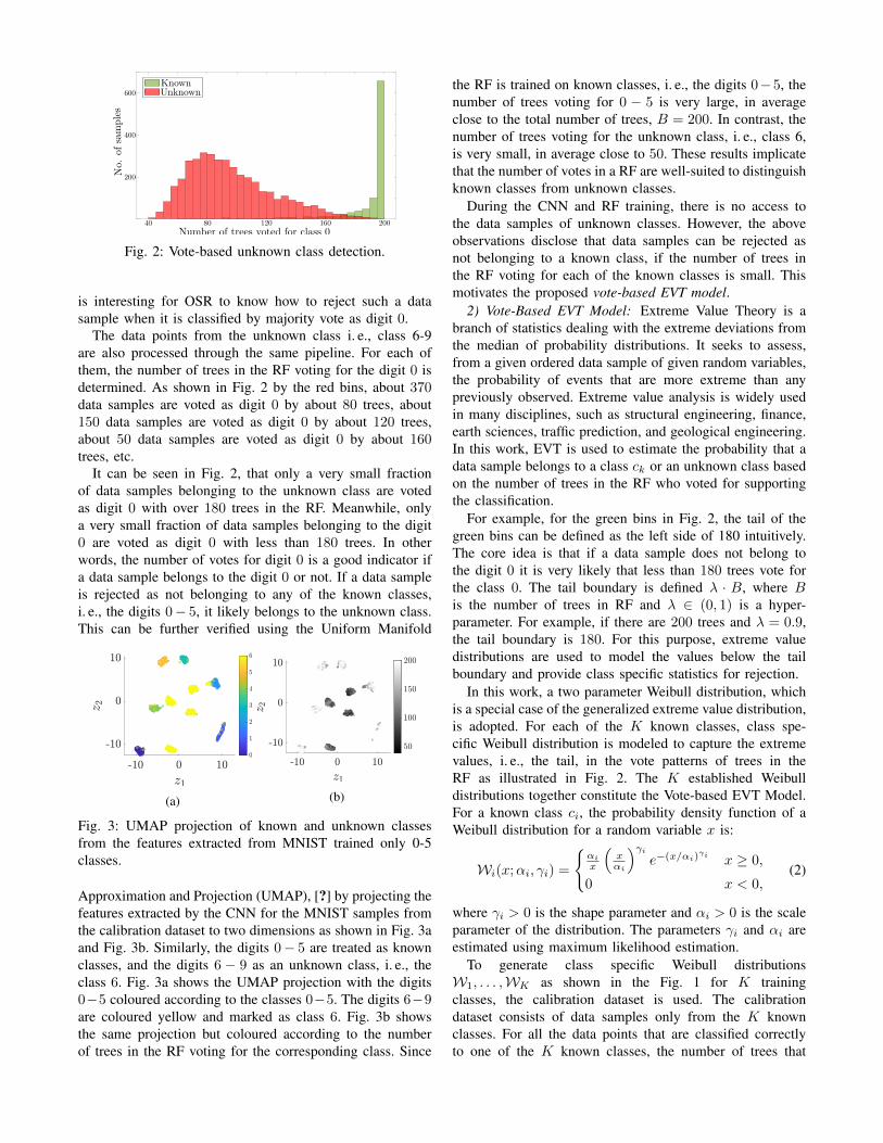
Fig. 2: Vote-based unknown class detection.

is interesting for OSR to know how to reject such a datasample when it is classified by majority vote as digit 0.

The data points from the unknown class i. e., class 6-9are also processed through the same pipeline. For each ofthem, the number of trees in the RF voting for the digit 0 isdetermined. As shown in Fig. 2 by the red bins, about 370data samples are voted as digit 0 by about 80 trees, about150 data samples are voted as digit 0 by about 120 trees,about 50 data samples are voted as digit 0 by about 160trees, etc.

It can be seen in Fig. 2, that only a very small fractionof data samples belonging to the unknown class are votedas digit 0 with over 180 trees in the RF. Meanwhile, onlya very small fraction of data samples belonging to the digit0 are voted as digit 0 with less than 180 trees. In otherwords, the number of votes for digit 0 is a good indicator ifa data sample belongs to the digit 0 or not. If a data sampleis rejected as not belonging to any of the known classes,i. e., the digits 0− 5, it likely belongs to the unknown class.This can be further verified using the Uniform Manifold

(a) (b)

Fig. 3: UMAP projection of known and unknown classesfrom the features extracted from MNIST trained only 0-5classes.

Approximation and Projection (UMAP), [?] by projecting thefeatures extracted by the CNN for the MNIST samples fromthe calibration dataset to two dimensions as shown in Fig. 3aand Fig. 3b. Similarly, the digits 0− 5 are treated as knownclasses, and the digits 6 − 9 as an unknown class, i. e., theclass 6. Fig. 3a shows the UMAP projection with the digits0−5 coloured according to the classes 0−5. The digits 6−9are coloured yellow and marked as class 6. Fig. 3b showsthe same projection but coloured according to the numberof trees in the RF voting for the corresponding class. Since

the RF is trained on known classes, i. e., the digits 0−5, thenumber of trees voting for 0 − 5 is very large, in averageclose to the total number of trees, B = 200. In contrast, thenumber of trees voting for the unknown class, i. e., class 6,is very small, in average close to 50. These results implicatethat the number of votes in a RF are well-suited to distinguishknown classes from unknown classes.

During the CNN and RF training, there is no access tothe data samples of unknown classes. However, the aboveobservations disclose that data samples can be rejected asnot belonging to a known class, if the number of trees inthe RF voting for each of the known classes is small. Thismotivates the proposed vote-based EVT model.

2) Vote-Based EVT Model: Extreme Value Theory is abranch of statistics dealing with the extreme deviations fromthe median of probability distributions. It seeks to assess,from a given ordered data sample of given random variables,the probability of events that are more extreme than anypreviously observed. Extreme value analysis is widely usedin many disciplines, such as structural engineering, finance,earth sciences, traffic prediction, and geological engineering.In this work, EVT is used to estimate the probability that adata sample belongs to a class ck or an unknown class basedon the number of trees in the RF who voted for supportingthe classification.

For example, for the green bins in Fig. 2, the tail of thegreen bins can be defined as the left side of 180 intuitively.The core idea is that if a data sample does not belong tothe digit 0 it is very likely that less than 180 trees vote forthe class 0. The tail boundary is defined λ · B, where Bis the number of trees in RF and λ ∈ (0, 1) is a hyper-parameter. For example, if there are 200 trees and λ = 0.9,the tail boundary is 180. For this purpose, extreme valuedistributions are used to model the values below the tailboundary and provide class specific statistics for rejection.

In this work, a two parameter Weibull distribution, whichis a special case of the generalized extreme value distribution,is adopted. For each of the K known classes, class spe-cific Weibull distribution is modeled to capture the extremevalues, i. e., the tail, in the vote patterns of trees in theRF as illustrated in Fig. 2. The K established Weibulldistributions together constitute the Vote-based EVT Model.For a known class ci, the probability density function of aWeibull distribution for a random variable x is:

Wi(x;αi, γi) =

{αix

(xαi

)γie−(x/αi)

γix ≥ 0,

0 x < 0,(2)

where γi > 0 is the shape parameter and αi > 0 is the scaleparameter of the distribution. The parameters γi and αi areestimated using maximum likelihood estimation.

To generate class specific Weibull distributionsW1, . . . ,WK as shown in the Fig. 1 for K trainingclasses, the calibration dataset is used. The calibrationdataset consists of data samples only from the K knownclasses. For all the data points that are classified correctlyto one of the K known classes, the number of trees that

voted for each correctly classified class is collected in thesets S1, . . . , SK , with Sk = {s1

k, . . . , sMk

k }, where, andMk is the number of scenarios belonging to class ck inthe calibration dataset. For a class ck, as only the extremevalues are of interest, Sk is sorted in the ascending orderand only vales below the tail boundary from the sorted Skare chosen for Weibull modelling. To set the tail boundary,first a filter using λ is done to remove highly confident datapoints which cannot belong to the unknown class basedon confidence score from Eq. (1), i. e., P (ck|qj ,θr) < λ.The remaining data points in Sk are used for estimating theclass specific Weibull parameters αk and γk by maximumlikelihood estimation.

D. Unknown Class PredictionAs discussed, the 3D CNN and RF have been trained

using the training dataset, and the vote-based EVT modeli. e., class specific Weibull models, has been learned usingthe calibration dataset. Recall that the training and calibrationdatasets contain data samples of known classes only. The testdata, or any new data samples collected in an application,includes data samples of both known and unknown classes.For each data sample in the test data, the 3D CNN, RFand voted-based EVT model are used to predict whether itbelongs to the unknown class or not.

Given a data sample Gj in the test dataset, it is first pro-cessed using the 3D CNN and the RF. Then, it is processedby the vote-based EVT model. As discussed, the vote-basedEVT model consists of Wi(αi, γi) for all K known classes.The cumulative probability that Gj belongs to class ci iscalculated by:

P (ci|sji , αi, γi) =

{1− e−(sji/αi)

γi, if sji > 0

0, otherwise.(3)

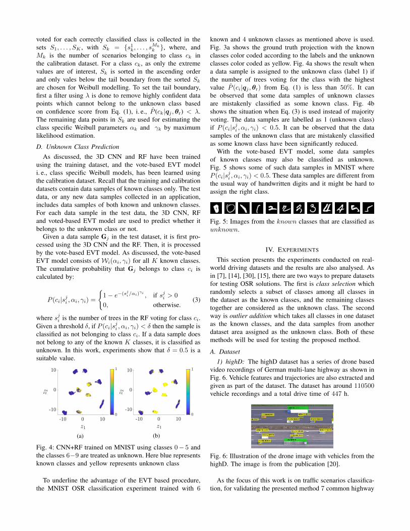
where sji is the number of trees in the RF voting for class ci.Given a threshold δ, if P (ci|sji , αi, γi) < δ then the sample isclassified as not belonging to class ci. If a data sample doesnot belong to any of the known K classes, it is classified asunknown. In this work, experiments show that δ = 0.5 is asuitable value.

(a) (b)

Fig. 4: CNN+RF trained on MNIST using classes 0− 5 andthe classes 6−9 are treated as unknown. Here blue representsknown classes and yellow represents unknown class

To underline the advantage of the EVT based procedure,the MNIST OSR classification experiment trained with 6

known and 4 unknown classes as mentioned above is used.Fig. 3a shows the ground truth projection with the knownclasses color coded according to the labels and the unknownclasses color coded as yellow. Fig. 4a shows the result whena data sample is assigned to the unknown class (label 1) ifthe number of trees voting for the class with the highestvalue P (ci|qj ,θr) from Eq. (1) is less than 50%. It canbe observed that some data samples of unknown classesare mistakenly classified as some known class. Fig. 4bshows the situation when Eq. (3) is used instead of majorityvoting. The data samples are labelled as 1 (unknown class)if P (ci|sji , αi, γi) < 0.5. It can be observed that the datasamples of the unknown class that are mistakenly classifiedas some known class have been significantly reduced.

With the vote-based EVT model, some data samplesof known classes may also be classified as unknown.Fig. 5 shows some of such data samples in MNIST whereP (ci|sji , αi, γi) < 0.5. These data samples are different fromthe usual way of handwritten digits and it might be hard toassign the right class.

Fig. 5: Images from the known classes that are classified asunknown.

IV. EXPERIMENTS

This section presents the experiments conducted on real-world driving datasets and the results are also analysed. Asin [7], [14], [30], [15], there are two ways to prepare datasetsfor testing OSR solutions. The first is class selection whichrandomly selects a subset of classes among all classes inthe dataset as the known classes, and the remaining classestogether are considered as the unknown class. The secondway is outlier addition which takes all classes in one datasetas the known classes, and the data samples from anotherdataset area assigned as the unknown class. Both of thesemethods will be used for testing the proposed method.

A. Dataset

1) highD: The highD dataset has a series of drone basedvideo recordings of German multi-lane highway as shown inFig. 6. Vehicle features and trajectories are also extracted andgiven as part of the dataset. The dataset has around 110500vehicle recordings and a total drive time of 447 h.

Fig. 6: Illustration of the drone image with vehicles from thehighD. The image is from the publication [20].

As the focus of this work is on traffic scenarios classifica-tion, for validating the presented method 7 common highway

(a) Ego - Following (b) Ego - Left Lane Change (c) Ego - Right Lane Change (d) Leader - Cutin from Right

(e) Leader - Cutin from Left (f) Leader - Cutout from Right (g) Leader - Cutout from Left

Fig. 7: Traffic scenario classes from highD. Here, the blue car is the ego vehicle and red cars are the traffic participants.

scenario classes as shown in Fig. 7 are extracted from thehighD dataset. The 7 classes are as follows:

• Ego - Following• Ego - Right lane change• Ego - Left lane change• Leader - Cutin from left• Leader - Cutin from right• Leader - Cutout to left• Leader - Cutout to rightAs described in III-A, THW< 4s is used as the crite-

rion for finding relevant scenarios where ego vehicle has aleading vehicle. The environment at each time instance isrepresented with Gt of span 15m × 200m and a resolutionof 0.5m × 1m. The interval t0 − tlb and ∆t used in thiswork are 1.8s and 0.2s respectively. So, a traffic scenariois represented with G of size 30 × 200 × 10. The grids aregenerated in an ego-centric fashion. In total 4480 scenarioswere extracted, where the split of dataset is 70% for training,10% for calibration and 20% for testing.

2) OpenTraffic: OpenTraffic is also a drone based dataset.Unlike highD, OpenTraffic focuses on roundabouts as shownin Fig 8. Similar to highD, as a post processing step vehiclefeatures and trajectories can be extracted. The OpenTrafficdataset is not labelled and will be used for the outlieraddition experiment, where all the data samples from theOpenTraffic dataset are considered as one unknown class.The scenario extraction and representation of the OpenTraffic

Fig. 8: Illustration of the drone image with vehicles from theOpenTraffic. The image is from the publication [21].

dataset is also done in the same way as the highD dataset asmentioned above.

B. Implementation Details

The 3D CNN architecture used in this work is similar tothe one used in [27] for video classification. The architecturedetails are given in the Table. I. For training, Adam [31]

optimiser is used and a batch size of 32 is chosen. The RFfor the vote-based method is trained with B = 200 trees.But as shown in the ablation study in Section V-.3, B has noinfluence on OSR performance atleast from the values 100and above. If the output of the CNN has L features, i. e.,q ∈ RL, the RF is fully-grown by selecting

√L features as

suggested in [?] to find the split rule for each node in eachtree of the RF. In the vote-based EVT model, the hyper-parameter λ is 0.9 as discussed in Section III-C.2 and δ isset to be 0.5 as discussed in Section III-D. The influence ofthe parameter δ is also discussed in the ablation study.

layer kernel stride input sizeconv1 4× 12× 3 1× 1× 1 30× 200× 10× 1

maxpool1 3× 3× 1 1× 1× 1 27× 189× 8× 8dropout1 (0.25) - - 9× 63× 8× 8

conv2 4× 8× 3 1× 1× 1 9× 63× 8× 8maxpool2 2× 3× 1 1× 1× 1 6× 56× 6× 6

dropout2 (0.25) - - 3× 18× 6× 6conv3 4× 12× 3 1× 1× 1 3× 18× 6× 6flatten - - 1020dense - - 500dense - - K

TABLE I: 3D CNN architecture details.

C. Baselines

The baseline methods used in this work to compare theOSR performance are

• Openmax [13], a re-calibrated softmax score based onthe per class EVT distribution of the class-wise featuredistances

• DOC [14], a normal CNN based classification networkwith a sigmoid layer at the end for OSR

• Softmax (Naive) and RF-conf (Naive), a rejectionthreshold of 0.5 is applied on the maximum softmaxscore and confidence score from Eq. (1) to distinguishunknown class and known classes

Compared to works mentioned above, the presented work inthis paper is an ensemble based and the spread of vote patternamong the ensembles is used as a measure of uncertainty.

D. Evaluation Metrics

The Macro-average of F -score is used as the metric forevaluating the OSR solutions. The F -score is the harmonic

mean of precision and recall,

F -score = 2 · precision · recallprecision + recall

(4)

where, recall = TPTP+FN and recall = TP

TP+FP . Here,TP, FP and FN are the true positives, false positives andfalse negatives respectively. The Macro-average of F -scoreis computed by taking the average of the F -scores for eachclass. The score values vary from 0 to 1, with 1 being thebest score.

E. Class Selection

This section reports the experiments where the highDdataset is prepared by the class selection method. Amongthe 7 labelled classes, 4 of them are retained as knownand the other 3 classes are treated as the unknown class.The class selection is repeated 5 times and each time the4 known classes are randomly selected. The 3D CNN, RFand the vote-based models are trained only on the 4 knownclasses. The ratio of known to unknown classes are alsovaried and the results are analysed in the ablation study. TheMacro-average of F -score with the standard deviations arepresented in Table II. The proposed vote-based EVT Modelis compared against baselines: Openmax, DOC, Softmax(Naive) and RF-conf (Naive). A larger score and a smallerstandard deviation indicate better performance. The resultsshow that the proposed vote-based EVT Model providesbetter and reliable performance in the conducted experiment.

TABLE II: Macro-average of F -score (class selection).

Method highD - 4 Known vs 3 UnknownSoftmax (Naive) 0.642±0.013

Openmax 0.71±0.017DOC 0.692±0.019

Rf-conf (Naive) 0.635±0.012Vote-based EVT 0.77±0.017

F. Outlier Addition

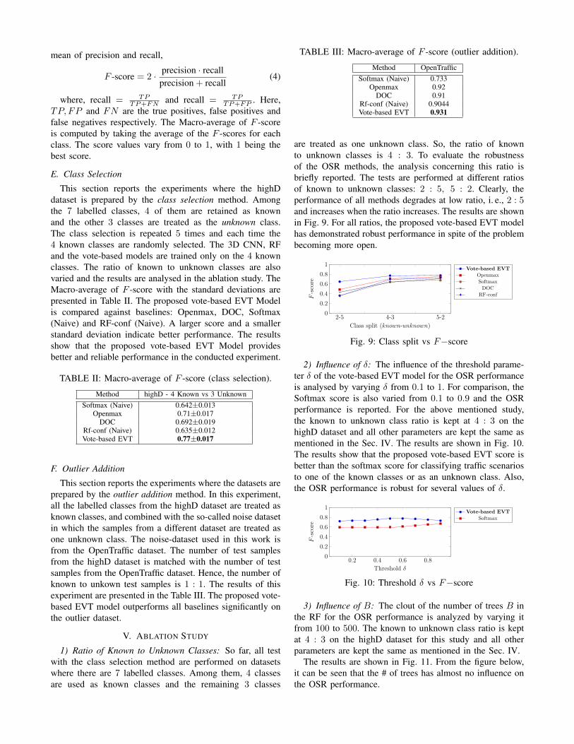
This section reports the experiments where the datasets areprepared by the outlier addition method. In this experiment,all the labelled classes from the highD dataset are treated asknown classes, and combined with the so-called noise datasetin which the samples from a different dataset are treated asone unknown class. The noise-dataset used in this work isfrom the OpenTraffic dataset. The number of test samplesfrom the highD dataset is matched with the number of testsamples from the OpenTraffic dataset. Hence, the number ofknown to unkown test samples is 1 : 1. The results of thisexperiment are presented in the Table III. The proposed vote-based EVT model outperforms all baselines significantly onthe outlier dataset.

V. ABLATION STUDY

1) Ratio of Known to Unknown Classes: So far, all testwith the class selection method are performed on datasetswhere there are 7 labelled classes. Among them, 4 classesare used as known classes and the remaining 3 classes

TABLE III: Macro-average of F -score (outlier addition).

Method OpenTrafficSoftmax (Naive) 0.733

Openmax 0.92DOC 0.91

Rf-conf (Naive) 0.9044Vote-based EVT 0.931

are treated as one unknown class. So, the ratio of knownto unknown classes is 4 : 3. To evaluate the robustnessof the OSR methods, the analysis concerning this ratio isbriefly reported. The tests are performed at different ratiosof known to unknown classes: 2 : 5, 5 : 2. Clearly, theperformance of all methods degrades at low ratio, i. e., 2 : 5and increases when the ratio increases. The results are shownin Fig. 9. For all ratios, the proposed vote-based EVT modelhas demonstrated robust performance in spite of the problembecoming more open.

2-5 4-3 5-20

0.2

0.4

0.6

0.8

1

Class split (known-unknown)

F-score

Vote-based EVTOpenmaxSoftmaxDOC

RF-conf

Fig. 9: Class split vs F−score

2) Influence of δ: The influence of the threshold parame-ter δ of the vote-based EVT model for the OSR performanceis analysed by varying δ from 0.1 to 1. For comparison, theSoftmax score is also varied from 0.1 to 0.9 and the OSRperformance is reported. For the above mentioned study,the known to unknown class ratio is kept at 4 : 3 on thehighD dataset and all other parameters are kept the same asmentioned in the Sec. IV. The results are shown in Fig. 10.The results show that the proposed vote-based EVT score isbetter than the softmax score for classifying traffic scenariosto one of the known classes or as an unknown class. Also,the OSR performance is robust for several values of δ.

0.2 0.4 0.6 0.80

0.2

0.4

0.6

0.8

1

Threshold δ

F-score

Vote-based EVTSoftmax

Fig. 10: Threshold δ vs F−score

3) Influence of B: The clout of the number of trees B inthe RF for the OSR performance is analyzed by varying itfrom 100 to 500. The known to unknown class ratio is keptat 4 : 3 on the highD dataset for this study and all otherparameters are kept the same as mentioned in the Sec. IV.

The results are shown in Fig. 11. From the figure below,it can be seen that the # of trees has almost no influence onthe OSR performance.

100 200 300 400 5000

0.2

0.4

0.6

0.8

1

# of Trees B

F-score

Vote-based EVT

Fig. 11: # of Trees B vs F−score

VI. CONCLUSIONS

OSR is an open problem of traffic scenario classificationeven though it is of high practical importance for autonomousdriving. This work proposes a combination of 3D CNN andthe RF algorithm along with extreme value theory to addressthe OSR task. The proposed solution, named vote-based EVTmethod, is featured by exploring the vote patterns of decisiontrees in RF for known classes and applying EVT to detect theunknown classes. Extensive tests on highD and OpenTrafficdatasets have verified the advantages of the new solutioncompared to state-of-the-art methods.

.

ACKNOWLEDGMENT

This work is supported by Bavarian State Ministry for Sci-ence and Art under the funding code VIII.2-F1116.IN/18/2.

REFERENCES

[1] H. Winner, S. Hakuli, F. Lotz, and C. Singer, Handbook of DriverAssistance Systems: Basic Information, Components and Systems forActive Safety and Comfort, 1st ed. Springer Publishing Company,Incorporated, 2015.

[2] S. International, Taxonomy and Definitions for Terms Related toOn-Road Motor Vehicle Automated Driving Systems, j3016 ed., 2014.

[3] A. Chaulwar, M. Botsch, and W. Utschick, “A machine learningbased biased-sampling approach for planning safe trajectories incomplex, dynamic traffic-scenarios,” in 2017 IEEE Intelligent VehiclesSymposium (IV), June 2017, pp. 297–303.

[4] F. Kruber, J. Wurst, and M. Botsch, “An unsupervised random forestclustering technique for automatic traffic scenario categorization,” 112018, pp. 2811–2818.

[5] I. Cara and E. d. Gelder, “Classification for safety-critical car-cyclistscenarios using machine learning,” in 2015 IEEE 18th InternationalConference on Intelligent Transportation Systems, Sep. 2015, pp.1995–2000.

[6] T. Gindele, S. Brechtel, and R. Dillmann, “Learning context sensitivebehavior models from observations for predicting traffic situations,”in 16th International IEEE Conference on Intelligent TransportationSystems (ITSC 2013), Oct 2013, pp. 1764–1771.

[7] A. Bendale and T. E. Boult, “Towards open world recognition,”CoRR, vol. abs/1412.5687, 2014. [Online]. Available: http://arxiv.org/abs/1412.5687

[8] L. P. Jain, W. J. Scheirer, and T. E. Boult, “Multi-class open setrecognition using probability of inclusion,” in Computer Vision –ECCV 2014, D. Fleet, T. Pajdla, B. Schiele, and T. Tuytelaars, Eds.Cham: Springer International Publishing, 2014, pp. 393–409.

[9] P. Oza and V. M. Patel, “Deep cnn-based multi-task learning foropen-set recognition,” CoRR, vol. abs/1903.03161, 2019. [Online].Available: http://arxiv.org/abs/1903.03161

[10] S. Rebuffi, A. Kolesnikov, and C. H. Lampert, “icarl: Incrementalclassifier and representation learning,” CoRR, vol. abs/1611.07725,2016. [Online]. Available: http://arxiv.org/abs/1611.07725

[11] Y. Wu, Y.-J. Chen, L. Wang, Y. Ye, Z. Liu, Y. Guo, and Y. Fu, “Largescale incremental learning,” 2019 IEEE/CVF Conference on ComputerVision and Pattern Recognition (CVPR), pp. 374–382, 2019.

[12] W. J. Scheirer, L. P. Jain, and T. E. Boult, “Probability models for openset recognition,” IEEE Transactions on Pattern Analysis and MachineIntelligence, vol. 36, no. 11, pp. 2317–2324, Nov 2014.

[13] A. Bendale and T. E. Boult, “Towards open set deep networks,”CoRR, vol. abs/1511.06233, 2015. [Online]. Available: http://arxiv.org/abs/1511.06233

[14] L. Shu, H. Xu, and B. Liu, “DOC: deep open classification of textdocuments,” CoRR, vol. abs/1709.08716, 2017. [Online]. Available:http://arxiv.org/abs/1709.08716

[15] P. Oza and V. M. Patel, “C2AE: class conditioned auto-encoder foropen-set recognition,” CoRR, vol. abs/1904.01198, 2019. [Online].Available: http://arxiv.org/abs/1904.01198

[16] P. R. Mendes-Junior, R. M. de Souza, R. de Oliveira Werneck,B. V. Stein, D. V. Pazinato, W. R. de Almeida, O. A. B. Penatti,R. da Silva Torres, and A. Rocha, “Nearest neighbors distance ratioopen-set classifier,” Machine Learning, vol. 106, pp. 359–386, 2016.

[17] H. Zhang and V. M. Patel, “Sparse representation-based open setrecognition,” CoRR, vol. abs/1705.02431, 2017. [Online]. Available:http://arxiv.org/abs/1705.02431

[18] Z. Ge, S. Demyanov, Z. Chen, and R. Garnavi, “Generative openmaxfor multi-class open set classification,” CoRR, vol. abs/1707.07418,2017. [Online]. Available: http://arxiv.org/abs/1707.07418

[19] L. Neal, M. Olson, X. Z. Fern, W.-K. Wong, and F. Li, “Open setlearning with counterfactual images,” in ECCV, 2018.

[20] R. Krajewski, J. Bock, L. Kloeker, and L. Eckstein, “The highddataset: A drone dataset of naturalistic vehicle trajectories on germanhighways for validation of highly automated driving systems,” in 201821st International Conference on Intelligent Transportation Systems(ITSC), 2018, pp. 2118–2125.

[21] F. Kruber, E. Sanchez Morales, S. Chakraborty, and M. Botsch,“Vehicle Position Estimation with Aerial Imagery from UnmannedAerial Vehicles,” in 2020 IEEE Intelligent Vehicles Symposium (IV),2020.

[22] M. Reichel, M. Botsch, R. Rauschecker, K. Siedersberger, andM. Maurer, “Situation aspect modelling and classification usingthe scenario based random forest algorithm for convoy mergingsituations,” in 13th International IEEE Conference on IntelligentTransportation Systems, Sep. 2010, pp. 360–366.

[23] H. Beglerovic, J. Ruebsam, S. Metzner, and M. Horn, “Polar occu-pancy map - a compact traffic representation for deep learning sce-nario classification,” in 2019 IEEE Intelligent Transportation SystemsConference (ITSC), 2019, pp. 4197–4203.

[24] A. Khosroshahi, E. Ohn-Bar, and M. M. Trivedi, “Surround vehiclestrajectory analysis with recurrent neural networks,” in 2016 IEEE19th International Conference on Intelligent Transportation Systems(ITSC), 2016, pp. 2267–2272.

[25] S. Lefevre, D. Vasquez, and C. Laugier, “A survey onmotion prediction and risk assessment for intelligent vehicles,”ROBOMECH Journal, vol. 1, no. 1, p. 1, 2014. [Online]. Available:https://hal.inria.fr/hal-01053736

[26] S. Ulbrich, T. Menzel, A. Reschka, F. Schuldt, and M. Maurer,“Defining and substantiating the terms scene, situation, and scenariofor automated driving,” in 2015 IEEE 18th International Conferenceon Intelligent Transportation Systems, Sep. 2015, pp. 982–988.

[27] S. Ji, W. Xu, M. Yang, and K. Yu, “3d convolutional neural networksfor human action recognition,” IEEE Transactions on Pattern Analysisand Machine Intelligence, vol. 35, pp. 221–231, 2010.

[28] D. Tran, L. Bourdev, R. Fergus, L. Torresani, and M. Paluri, “Learningspatiotemporal features with 3d convolutional networks,” in 2015IEEE International Conference on Computer Vision (ICCV), 2015,pp. 4489–4497.

[29] Y. LeCun and C. Cortes, “MNIST handwritten digit database,” 2010.[Online]. Available: http://yann.lecun.com/exdb/mnist/

[30] R. Yoshihashi, W. Shao, R. Kawakami, S. You, M. Iida, and T. Nae-mura, “Classification-reconstruction learning for open-set recognition,”in IEEE Conference on Computer Vision and Pattern Recognition,CVPR 2019, Long Beach, CA, USA, June 16-20, 2019. ComputerVision Foundation / IEEE, 2019, pp. 4016–4025.

[31] D. P. Kingma and J. Ba, “Adam: A method for stochasticoptimization,” 2014, cite arxiv:1412.6980Comment: Published asa conference paper at the 3rd International Conference forLearning Representations, San Diego, 2015. [Online]. Available:http://arxiv.org/abs/1412.6980