Open Systems for the Working Mathematician

Owen Lynch

April 29, 2020

Contents

1 Introduction 21.1 The Purpose of this Review . . . . . . . . . . . . . . . . . . . 21.2 What is a System? . . . . . . . . . . . . . . . . . . . . . . . . 21.3 What is an Open System? . . . . . . . . . . . . . . . . . . . . 4

2 Material 62.1 Decorated Graphs . . . . . . . . . . . . . . . . . . . . . . . . 62.2 Chemical Reactions . . . . . . . . . . . . . . . . . . . . . . . . 62.3 Linear Algebra . . . . . . . . . . . . . . . . . . . . . . . . . . 8

3 Monoidal Categories 83.1 Overview . . . . . . . . . . . . . . . . . . . . . . . . . . . . . 83.2 Monoidal Functors . . . . . . . . . . . . . . . . . . . . . . . . 113.3 Symmetric Monoidal Categories . . . . . . . . . . . . . . . . . 113.4 Petri Nets as Presentations of SSMCs . . . . . . . . . . . . . 12

4 String Diagrams 134.1 String Diagrams as Dual to Commutative Diagrams . . . . . 134.2 String Diagrams as Histories . . . . . . . . . . . . . . . . . . . 144.3 String Diagrams As Circuits . . . . . . . . . . . . . . . . . . . 174.4 The Braid Category . . . . . . . . . . . . . . . . . . . . . . . 184.5 Linear Algebra in String Diagrams . . . . . . . . . . . . . . . 20

5 Cospans 255.1 Basic Cospans . . . . . . . . . . . . . . . . . . . . . . . . . . . 255.2 Structured Cospans . . . . . . . . . . . . . . . . . . . . . . . . 275.3 Categories of Open Systems . . . . . . . . . . . . . . . . . . . 285.4 Corelations . . . . . . . . . . . . . . . . . . . . . . . . . . . . 29

1

6 Semantic Functors 296.1 Steady State Solutions for Resistor Networks . . . . . . . . . 306.2 Open Dynamical Systems . . . . . . . . . . . . . . . . . . . . 316.3 Rate Equation for Petri Nets . . . . . . . . . . . . . . . . . . 34

1 Introduction

1.1 The Purpose of this Review

In this review, we attempt to collect and summarize recent work that has beenhappening across the field of applied category theory around open systems.There is a good deal of work put into making open systems accessible to thescientist who was previously unfamiliar with categories. Therefore, in orderto make an original contribution, in this review we attempt to make opensystems accessible to the category theorist who was previously unfamiliarwith science.

This review is organized in a grid fashion. In the second section, we willintroduce three application domains for the later study of theory. In eachsubsequent section, when we introduce a new concept we will talk about howthat subject interfaces with all three application domains. Our hope is thatthis will congeal the concepts presented, and make it more clear how they tietogether.

Before we dive into the math, however, we need to talk about what opensystems mean philosophically, and before we do that, we need to talk aboutsystems.

1.2 What is a System?

This has an easy answer: a system is an object whose class of behaviors wewant to study. This seems unsatisfying, but from a mathematical perspectivewhat this is saying is that “system” is a term left undefined, like “point” or“line”. We will develop a theory around “systems” that gives them meaningfrom context (though this theory will not be nearly as rigorous as Euclideangeometry).

We can apply various adjectives to “system” that narrow the type ofbehavior associated with a system. For instance, one large class of systemsis “dynamical systems”. Dynamical systems are characterized by a focus onevolving a system over time. Typically, this is done by means of differentialequations.

2

Example 1. Consider the cylinder S1 × R, which we use to represent thepossible position, velocity pairs of a pendulum. Let (θ, θ̇) be coordinatesfor the cylinder. Then the evolution of (θ, θ̇) is governed by the differentialequations

∂

∂tθ̇ = cos(θ)

∂

∂tθ = θ̇

These differential equations are a presentation of a section of the tangent bun-dle of S1 ×R. We use this section to generate a 1-parameter diffeomorphismgroup acting on S1 ×R.

There are more adjectives that we can use to describe the system above:it is continuous time, and it is deterministic. Its state space is S1 ×R, andits time axis is R. Mechanics is the study of continuous time, deterministicdynamical systems.

In general, a dynamical system will have a 1-parameter monoid acting onit. This monoid will typically be R≥0 or N, but it could be R or Z. Thatis, if BM is a category with one object and morphisms given by elements ofM , and C is some category like the category of manifolds, or the categoryof metric spaces, or the category of vector spaces, then the formal objectcorresponding to an evolution of c ∈ C is a functor from BM to C that sendsthe one object of BT to c.

Example 2. Consider a matrix T ∈ RZ×Z defined by Ti,i+1 = 0.5, Ti,i−1 = 0.5,Ti,j = 0 otherwise. Then we define an action of N on ∆Z, the space ofprobability distributions on the integers, by k 7→ T k. This represents arandom walk on the set of integers. If p ∈ ∆Z is a probability distributionover Z, then T kp is the probability distribution of the state of the randomwalker after k steps, if the state of the random walker was originally distributedas p.

This is a discrete time, stochastic dynamical system. Its state space is Z,and its time axis is N. Note that one could also look at this as a deterministicsystem with state space ∆Z (the set of probability distributions over Z); ingeneral a stochastic system can also be viewed as a deterministic systemwhere the state space is the set of probability distributions over the originalstate space. The difference is the approach: the study of stochastic systemsuses methods of probability theory because we typically care about questionsabout our systems that have probabilisitc answers.

There are also static systems, which can be viewed as special cases ofdynamical systems that don’t evolve over time. A dynamical system with

3

arbitrary time axis A and state space E can be viewed as a static systemwith state space EA.

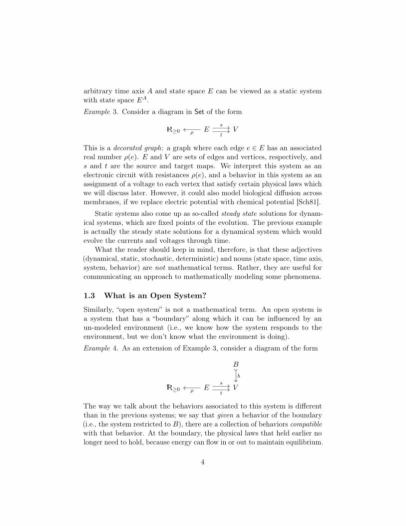
Example 3. Consider a diagram in Set of the form

R≥0 E Vρ

s

t

This is a decorated graph: a graph where each edge e ∈ E has an associatedreal number ρ(e). E and V are sets of edges and vertices, respectively, ands and t are the source and target maps. We interpret this system as anelectronic circuit with resistances ρ(e), and a behavior in this system as anassignment of a voltage to each vertex that satisfy certain physical laws whichwe will discuss later. However, it could also model biological diffusion acrossmembranes, if we replace electric potential with chemical potential [Sch81].

Static systems also come up as so-called steady state solutions for dynam-ical systems, which are fixed points of the evolution. The previous exampleis actually the steady state solutions for a dynamical system which wouldevolve the currents and voltages through time.

What the reader should keep in mind, therefore, is that these adjectives(dynamical, static, stochastic, deterministic) and nouns (state space, time axis,system, behavior) are not mathematical terms. Rather, they are useful forcommunicating an approach to mathematically modeling some phenomena.

1.3 What is an Open System?

Similarly, “open system” is not a mathematical term. An open system isa system that has a “boundary” along which it can be influenced by anun-modeled environment (i.e., we know how the system responds to theenvironment, but we don’t know what the environment is doing).

Example 4. As an extension of Example 3, consider a diagram of the form

B

R≥0 E V

b

ρ

s

t

The way we talk about the behaviors associated to this system is differentthan in the previous systems; we say that given a behavior of the boundary(i.e., the system restricted to B), there are a collection of behaviors compatiblewith that behavior. At the boundary, the physical laws that held earlier nolonger need to hold, because energy can flow in or out to maintain equilibrium.

4

There also may be no system behavior compatible with a boundary behavior,and we interpret this as the system enforcing a constraint on its boundary.

Example 5. Consider the same pendulum system, but now with an additionalterm added to the differential equation

∂

∂tθ̇ = cos(θ) + F (t)

∂

∂tθ = θ̇

This additional term represents an external force. We still end up with aevolution through time, but now it takes a slightly different form. That is,we care not just about the total time that the system has evolved for, butalso the starting and ending time. Therefore, our “action” is a functor fromR viewed as a poset: any morphism t −→ t′ gives a diffeomorphism from thecylinder to itself.

Example 6. Any closed system is an open system with empty boundary.

Just as a drunk searches for his keys under a lamp post because that’swhere he can see, scientists have concentrated on systems whose behaviorcan be studied in isolation, i.e. systems without boundary. This is because itis easier to make and test hypotheses when one does not have to worry aboutunmodeled interactions with the environment.

Classically, when systems that we want to model are open systems in thereal world, we get around their dependence on the environment by eitherneglecting it, or adding more parts of the environment to the model. Andin fact, when we are only concerned about one system, this is desirable: wewant to ask questions about a single system, so we add everything we knowabout that system in order to get the best picture possible.

However, when we explicitly model the environment to create a closedsystem, we lose the ability to compose the model that we have made with othermodels of the environment. This is the key feature of open systems: opensystems are most naturally discussed in a compositional framework whereone can “glue” two open systems together along a part of their boundary.

In short, just as dynamical systems are distinguished by an approach thatcares about time evolution, and stochastic systems are distinguished by anapproach that cares about nondeterminism, open systems are distinguishedby an approach that cares about compositionality. And that is where thecategory theory comes in.

5

2 Material

Here we introduce three examples that will run through this paper andillustrate each of the tools that we build. We will not be able to explain theseexamples thoroughly now, because we don’t have the right tools with whichto do so. However, keeping these examples in mind as we run through thedifferent tools for open systems will be useful.

2.1 Decorated Graphs

Fix a set D, which we will call the set of decorations. Then a decorated graphwith decorations D is a diagram in Set of the form

D E Vd s

t

The elements of E are called “edges”, and the elements of V are called“vertices”. Note that this definition of graph allows for self-edges and multipleedges, and edges are directed with a “source” s(e) and “target” t(e).

Each edge has an associated “decoration” d(e), which is an element of D.Example 7. A social network is a decorated graph. The set of decorations isthe set of labels for relationships between two people, for instance “parent”,“friend”, “boss”, “priest”, “doctor”, etc. Edges from a vertex to itself makesense in this context because someone could be their own boss, or their owndoctor. Additionally, two people could have several relationships with eachother, so there could be several edges between two vertices.

To build the category of decorated graphs over the decoration set D, letC be the following category:

d e nδ

τ

σ

Then take the subcategory of SetCop

where the objects are F such thatF (d) = D and the arrows are α such that αδ = 1D.

2.2 Chemical Reactions

Fix a finite set S, which we call the set of species. Then we call C = NS theset of complexes on S: a complex is an assignment of a natural number toeach species. A reaction is an element r of C × C: we call π1(c) the inputand π2(c) the output.

A Petri net is nothing more than a set of reactions.

6

H2

O2

H2O

Figure 1: A Petri net for making water.

R WPB D

Figure 2: A Petri net describing predator-prey interaction.

Example 8. Let S = {H2,O2,H2O}. Then

2H2 + O2 −→ 2H2O

is a reaction written down in the language of chemistry. We invite the readerto take a moment and think about how to parse this formula into the fomalismabove.

Example 9. Let S = {W,R}. In this case, W and R do not stand in formolecules; they stand in for wolves and rabbits. Then a standard predatorprey model can be expressed as

R + W −→ 2WR −→ 2RW −→

The first “reaction” represents predation and wolf reproduction. The as-sumption is that one rabbit is converted into one wolf, catalyzed by a wolfwhich “eats” the rabbit and “gives birth” to the new wolf. The second reac-tion is rabbit reproduction, in this case asexual: one rabbit splits into tworabbits. Finally, wolves occasionally die spontaneously. This is obviously asimplification, but even so this model can capture real population dynamics.

There is a neat diagram that one can associate to a Petri net, which onecan see in Figure 1 and Figure 2. The blue circles correspond to species,and the grey squares correspond to reactions. For each input to a reaction,there is an arrow coming from the corresponding species circle to the reaction

7

square, and for each output from a reaction, there is an arrow going from thereaction to the corresponding species.

A morphism of Petri nets is exactly like a graph morphism. That is,if (Sk, Rk, sk : Rk −→ N

Sk , tk : Rk −→ NSk), k ∈ {1, 2} are two Petri nets,

then a morphism between them is a function fS : S1 −→ S2 and a functionfR : R1 −→ R2 that commutes with source and target. If the Petri net isdecorated with rates, then we require that fR also preserves rates.

2.3 Linear Algebra

The reader should be familiar with Veck, the category of vector spaces over afield k. What might be less familiar is the the category of linear relations overa field k, which we call LinRelk. The objects in this category are vector spacesover k, and a morphism between U and V is a linear subspace R ⊆ U × V ,which is interpreted as a relation in a standard way. Then to composeR ⊆ U × V and S ⊆ V ×W , we define S ◦R by

{(u,w) ∈ U ×W | ∃v ∈ V such that (u, v) ∈ R and (v, w) ∈ S}.

We care about LinRelk because it is a convenient and simple category for thebehavior of open systems. An open system doesn’t have inputs and outputsin a traditional sense: rather it enforces constraints between different partsof its boundary.

For instance, an electronic circuit enforces a relationship between thevoltages of different nodes in the circuit. A Petri net enforces a relationshipbetween the quantities of different substances.

From a mathematical perspective as well, LinRelk has an interestingalgebraic presentation, which we will discuss later on.

3 Monoidal Categories

3.1 Overview

We will eventually compose systems by gluing them along part of theirboundary. However, before we do this, we first study composing systemsby just juxtaposing them and not worrying about the glue yet. The correctstructure for this sort of composition is a monoidal category.

Recall that a monoid can be viewed as a category with only one object.Classically, we don’t think about the single object, and we just think of themonoid as a set with an associative binary operation that has a unit. However,this definition as a one object 1-category is useful, because it makes monoidal

8

categories a natural generalization: a monoidal category is a 2-category withonly one object. Classically, we think of a monoidal category as a 1-categorythat has a binary operation on it satisfying certain laws about its interactionwith the arrows of the category. These laws are much easier to remember,and are more naturally derived, however, if one simply thinks of the monoidalcategory as a 2-category with only one object.

For the reader who has only passing familiarity with 2-categories, we willdo a brief review. A 2-category is composed of objects A,B, 1-morphismsf, g : A −→ B, and 2-morphisms α : f ⇒ g, that satisfy the following.

1. Hom(A,B) is a 1-category for any objects A,B, with objects the 1-morphisms and arrows the 2-morphisms.

2. For all objectsA,B,C, we have a functor ◦ : Hom(A,B)×Hom(B,C) −→Hom(A,C) such that:

(a) (− ◦ −) ◦ − and − ◦ (− ◦ −) are naturally isomorphic, and thisnatural isomorphism respects the Maclane pentagon identity.

(b) For every A, there exists 1A ∈ Hom(A,A) such that 1A ◦ −is naturally isomorphic to 1Hom(B,A), and − ◦ 1A is naturallyisomorphic to 1Hom(A,B) for all B.

We call a 2-category strict if the natural isomorphisms in 2a and 2bare equalities, and weak otherwise. It is an important theorem that any2-category is equivalent to a strict 2-category if we take the right notionof equivalence of 2-categories. This means that we don’t really have toworry about the difference between strict 2-categories and weak 2-categories.However, it is important to get in the habit of worrying about strict vs. weak,because it will be important for some structures later on.

Example 10. The category of categories and functors, Cat, has a natural2-category structure given by adding natural transformations as 2-morphisms.This is a strict 2-category.

A 2-category with one object, ∗, is comprised of a 1-category Hom(∗, ∗)along with an associative and unital binary operation, ◦ : Hom(∗, ∗) ×Hom(∗, ∗) −→ Hom(∗, ∗). Normally in this case, we call this operation ⊗instead of ◦, and reserve ◦ for composition of morphisms in Hom(∗, ∗). Wealso typically call the identity element I.

Example 11. In the above 2-category, take the subcategory with single object

9

FinSet, 1-morphisms generated by the basepoint functor,

F : FinSet −→ FinSet

A 7→ A t {∗}

and 2-morphisms being all natural transformations α : Fn ⇒ Fm. If wethink about this as a 1-category with a binary operation, this is a skeleton ofFinSet with the binary operation of disjoint union, i.e. the set of objects isisomorphic to N, and the binary operation is + with unit 0. This is a veryimportant monoidal category; we will call it (F ,+, 0).

One part of the definition of a monoidal category that is important toemphasize is the ability to compose morphisms sideways as well as vertically.That is, if (C,⊗, I) is a monoidal category, then we can compose morphismsas illustrated in the following diagram.

a b a⊗ b

⇒

c d c⊗ d

f g f⊗g

Holding with the general idea in category theory that the morphismsare more interesting than the objects, it is this structure on the arrows in amonoidal category that makes monoidal categories interesting.Example 12. Let C be a category with products and terminal objects. Thenif we let ⊗ be the product and I be the terminal object, it can be shown that(C,⊗, I) is a monoidal category. Similarly, we can do this with sums and theinitial object.Example 13. If R is a commutative ring, then (ModR,⊗R, R) is a monoidalcategory, where ⊗ is the normal tensor product.Example 14. The category of decorated graphs has coproducts (disjoint unionof nodes and edges), and initial object (the empty graph), and we customarilyuse the monoidal category structure given by this.Example 15. Veck can be viewed as a monoidal category (Veck,⊗, k) using thetensor product of vector spaces, or it can be viewed as a monoidal categegory(Veck,⊕, 0) using direct product. This second monoidal category structurealso works for LinRelk, as given R1 ⊆ V1 ×W1 and R2 ⊆ V2 ×W2, we canconstruct

R1 ×R2 ⊆ (V1 ×W1)× (V2 ×W2) ∼= (V1 × V2)× (W1 ×W2)

10

3.2 Monoidal Functors

The naive way to define a monoidal functor between (C,⊗, I) and (D,�, J)is to say that a monoidal functor is an ordinary functor F where

F (c1 ⊗ c2) = F (c1) � F (c2)

F (I) = J

However, this is too restrictive (this is what we call a strict monoidal functor).A more permissive way to define a monoidal functor is to require thatF (c1⊗ c2) ∼= F (c1)�F (c2) and that F (I) ∼= J , and that these isomorphismssatisfy some coherence conditions. This is the restriction of the notion of apseudofunctor between 2-categories, and is called a weak monoidal functor;to learn the details of the coherence conditions for pseudofunctors, we referthe reader to [Lei03].

It is important to note that while all 2-categories are equivalent to strict2-categories, not all monoidal functors are equivalent to strict monoidalfunctors.

3.3 Symmetric Monoidal Categories

Another example of when weakness is or isn’t important is when we try tomake an analogue of commutative monoids. If we require that a⊗ b = b⊗ a,not many categories satisfy this condition. Categories which do, we call “strictsymmetric monoidal categories”.

However, the requirement that (a, b) 7→ a ⊗ b and (a, b) 7→ b ⊗ a arenaturally isomorphic functors is much less restrictive, and is satisfied by manyimportant monoidal categories. In fact, this is the case for all of the exampleswe have given up to now. When this is true, we call the category a braidedmonoidal category, and we call the natural isomorphism the braiding. We willsee why this is a natural term and give an example later.

But that condition by itself is too loose. If αa,b : a ⊗ b −→ b ⊗ a are thecomponents of the natural isomorphism, then we want it to be the casethat αa,b is just “swapping” a and b, and if we swap them back with αb,a weshould end up in the same place we started with. That is, α · α, where · iscomposition of natural transformations, should be the identity. This is notalways true, but when it is true, we call the category a symmetric monoidalcategory.

Most of the categories that we expect the reader to be familiar with fallinto this designation. For instance, all of the categories with a monoidaloperation defined by product or coproduct are symmetric monoidal, and

11

the categories with a tensor product that is adjoint to the Hom functorare symmetric monoidal. We will use the symmetric monoidal structure ofcoproduct on the category of Petri nets and the category of electronic circuits.

3.4 Petri Nets as Presentations of SSMCs

Not only does that category of Petri nets have a symmetric monoidal struc-ture, but also an individual Petri net can be viewed as generating a (strict)symmetric monoidal category.

Recall that for any graph, we can make the “free category” on that graph.This construction is the left adjoint to the “forgetful functor” that takesa category to its underlying graph. Similarly, there is a functor from thecategory of strict symmetric monoidal categories to the category of monoidalgraphs (the category of graphs with a monoid structure on the nodes). Thisfunctor also has a left adjoint, which sends a monoidal graph to the free strictsymmetric monoidal category generated by edges in that graph.

Just like in the construction of a free category, the objects of the free strictsymmetric monoidal category are the same as the vertices of the monoidalgraph. However, a morphism in this category is more complicated. This isbecause there are two ways of composing morphism in a monoidal category:by tensor product, and by normal composition. The morphisms in the freestrict symmetric monoidal category are freely generated by both of theseoperations.

A Petri net can naturally be seen as a monoidal graph: the objects are theset of complexes, NS , and the arrows are the reactions. Even better: there isa functor from the category of Petri nets to the category of monoidal graphs.We can compose this functor with the functor from monoidal graphs to strictsymmetric monoidal categories, and we end up with a functor assigining astrict symmetric monoidal category to each Petri net. In this symmetricmonoidal category, we interpret a morphism from one complex to anothercomplex as a sequence of reactions. Each reaction applies to a subcomplex,and replaces that subcomplex with the result of that reaction. In this category,we say that the reaction generate the morphisms.

Note that this is not a full embedding. There are more morphisms in thecategory of strict symmetric monoidal categories. For instance, a morphismcould collapse a series of reactions to a single reaction, or expand a singlereaction to several reactions, neither of which are possible in the categoryof Petri networks. This allows one to potentially simplify a Petri net whilemaintaining essential properties. For more information, see [BC18].

We would give an example, however we do not yet have the right notation

12

to make this intuitive. Monoidal categories are confusing because there aretwo dimensions of composition: there is ordinary morpism composition f ◦ gand there is “sideways” morphism composition f ⊗ g. In order to fully makesense of this, we need new notation that captures these two dimensions, andthat brings us to our next section.

4 String Diagrams

In this section, we will present a new notation for working with monoidalcategories (and more generally, 2-categories), and we will give several inter-pretations of this notation in order help the reader develop an intuition forit and a facility for its use. The emphasis will be on notation rather thancategory theory. We will finish with a presentation of the category of linearrelations using string diagrams.

4.1 String Diagrams as Dual to Commutative Diagrams

In typical commutative diagrams, we draw objects as dots, 1-morphisms aslines, and 2-morphisms as regions. In the language of cell complexes, objectsare 0-cells, 1-morphisms are 1-cells, and 2-morphisms are 2-cells. Classically,this looks something like:

A B

f

g

α

where we imagine that α is a region filling in the space between f and g.This same diagram in string diagram notation would look like:

Often string diagrams are labelled with colors rather than symbols, butthis is merely an aesthetic change. The main difference is that what was ak-cell in the previous diagram is now a (2− k)-cell. A student of topologywill recognize this as Poincaré duality.

The commutative diagram had 0-cells A and B; the string diagram hascorresponding orange and green 2-cells. The commutative diagram had 1-cellsf and g, and the string diagram has corresponding blue and red 1-cells which

13

are perpendicular to the f and g in the commutative diagram. Finally, α,the one 2-cell in the original diagram, has become a 0-cell.

In the case of a monoidal category, there is only one object, so we mayleave the regions blank, and this is how we will write string diagrams for therest of this survey. We have introduced string diagrams in the more generalcontext of 2-categories in order to firmly disassociate 0-cells and objects inthe reader’s mind; we have found that this is the hardest thing to explainabout string diagrams.

One last thing we will note: we are not at all consistent in how we drawstring diagrams; each section will have a slightly different style. This isfor two reasons. The first is that “in the wild” there are many styles ofstring diagram, and it is important to recognize the commonalities and basicstructure between them. The second reason is that there are aspects of stringdiagrams that are better captured by one style than others.

4.2 String Diagrams as Histories

In the context of Petri nets there is another way of interpreting a stringdiagram. Recall that a Petri net is a presentation for a strict, symmetricmonoidal category. Each object in this monoidal category (i.e., 1-morphism ina 2-category with one object) is a complex, and each arrow (i.e. 2-morphism) isa sequence of reactions. A string diagram is a way of displaying a compositionof 2-morphisms, so in this context a string diagram is a way of displayingseveral reactions in sequence.

Before we go any farther, the reader is invited to look at Figure 3 andimagine how it might represent a sequence of reactions, if the green is H2,the red is O2, the blue is H2O, the black dot is the reaction

2H2 + O2 2H2O

and the white dot is the reverse reaction.The way we advise the reader to interpret such a diagram is as a time

history, flowing from bottom to top. Each horizontal slice of the diagramcorresponds to the state of the system at a point in time. This view ispictured in Figure 4.

For instance, slicing the diagram at the very bottom gives four greenthreads and 2 red threads, which corresponds to the complex 4H2 + 2O2.Then, as we move through time, reactions happen at distinct points, and

14

Figure 3: Water Formation

Figure 4: Sliced Water Formation

change the complex.1 The sequence of reactions is

4H2 + 2O2 2H2 + O2 + 2H2O 4H2O 2H2 + O2 + 2H2O

The reader may object that we are not worrying about the order in which thereactants are listed. This is because earlier we defined the monoidal categoryassociated with a Petri net to be strictly symmetric, so that H2 + O2 =O2 + H2. In the following section, this will not be true.

Now, the most important part of category theory is composition, and it isin composition where string diagrams start to really shine. We noted earlierthat it is hard to keep straight the two different types of composition in amonoidal category, that is f ⊗g and f ◦g. String diagrams solve this problemvery neatly. To tensor together two morphisms f and g, we simply put thetwo diagrams that represent them side by side.

In the “time-history” interpretation, horizontal composition signifies twotime histories happening in parallel, not affecting each other. Normal com-

1For the reader who has experience with Morse theory, the idea that the complex staysthe same except for at “critical points” should be familiar.

15

a c

b d

f g

a⊗ c

b⊗ d

f ⊗ g =

position is achieved by vertical stacking; the interpretation here is that twoprocesses happen in sequence.

=g ◦ f

g

f

There is one more ingredient that is necessary to interpret these diagrams.Namely, what is a plain wire? A fan of 0 might have have noticed that wegave diagrammatic interpretations for two types of composition, but we didnot give a diagrammatic interpretation for the other key part of a category:the identities. The identity for the monoidal composition is very simple, itlooks like this:

That is, the identity for the monoidal/horizontal composition is an emptydiagram.2 However, the identity for regular/vertical composition is not justa blank diagram. It is a straight wire with no decorations, or several straightwires. For instance, the following figure is the identity on H2O + H2 + O2.

It is the identity which allows us to apply a reaction to a subcomplex;if f is a reaction that has domain A, then we can apply f to the complex

2Actually, in the 2-category setting where we color the background, the monoidalidentity would be a monochromatic square.

16

A⊗B by tensoring f with 1B.There are more to string diagrams than particle-histories, however, so

the reader is advised to not get too attached to this interpretation. Themain take-away from this section should be the correspondence betweenthe graphical notation and the categorical operations: this is what will beimportant for the next section.

4.3 String Diagrams As Circuits

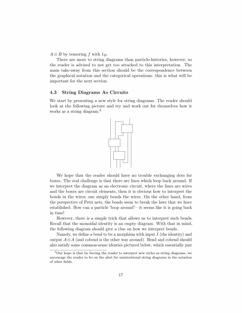
We start by presenting a new style for string diagrams. The reader shouldlook at the following picture and try and work out for themselves how itworks as a string diagram.3

We hope that the reader should have no trouble exchanging dots forboxes. The real challenge is that there are lines which loop back around. Ifwe interpret the diagram as an electronic circuit, where the lines are wiresand the boxes are circuit elements, then it is obvious how to interpret thebends in the wires; one simply bends the wires. On the other hand, fromthe perspective of Petri nets, the bends seem to break the laws that we haveestablished. How can a particle “loop around”—it seems like it is going backin time!

However, there is a simple trick that allows us to interpret such bends.Recall that the monoidal identity is an empty diagram. With that in mind,the following diagram should give a clue on how we interpret bends.

Namely, we define a bend to be a morphism with input I (the identity) andoutput A⊗A (and cobend is the other way around). Bend and cobend shouldalso satisfy some common-sense identies pictured below, which essentially just

3Our hope is that by forcing the reader to interpret new styles as string diagrams, weencourage the reader to be on the alert for unintentional string diagrams in the notationof other fields.

17

say that there are no “side-effects” to a bend; it is just a way of redirectingwires.

= =

=

Categorically speaking, bend and cobend are natural transformationsbetween the functors A 7→ A⊗A and A 7→ I, that satisfy the above laws.

We will refrain from a rigorous treatment of electrical circuits as stringdiagrams until after we have studied cospans.

4.4 The Braid Category

We promised earlier that we would discuss braided monoidal categories. Wenow have the notation to make the word “braided” intuitive. In a braidedmonoidal category, we write the braiding A ⊗ B ∼= B ⊗ A as one strandcrossing over another.

The inverse of the braiding is depicted by reversing the directions thatthe strands cross, and it should make intuitive sense why it is the inverse:one can imagine deforming the first diagram into the second without movingthe ends, if the strings are embedded in 3-space.

18

=

On the other hand, in a general braided monoidal category the belowequation does not hold.

=

If the string diagram is embedded in 3-space, then one cannot untanglethe two strands without moving the ends.4

The canonical example of a braided category is the braid category, whichis the free braided symmetric monoidal category on one object T . Notethat because it is a monoidal category, there are actually N objects in thiscategory, all tensor powers of the one generating objects. The morphismsin this category are generated by the identity and the braiding: a typicalmorphism in the braid category is pictured below.

If the reader has studied knot theory, the braid group should be familiar.It might be surprising to learn that the braid group on n strands has analgebraic presentation: it is the full subcategory of the braid category spannedby the object T⊗n.

4On the other hand, if the string diagram is embedded in 4-space, then one can untanglethe two strands. Somehow, this has to do with the distinction between braided monoidaland symmetric monoidal: the interested reader should consult [BS09] for an investigationof interesting alignments along these lines.

19

4.5 Linear Algebra in String Diagrams

The previous two examples have both been schematic. That is, we used stringdiagrams essentially as just fancy graphs. In this section, we will emphasizethe algebraic aspects of string diagrams; i.e. the ability for string diagramsto be used as a tool for computation.

Consider the category LinRelk. This has a monoidal structure given bydirect product, as we talked about before. We also claimed that LinRelkhad an interesting algebraic structure. In this section we will discuss thisalgebraic structure.

By algebraic structure, we mean that in the subcategory monoidallygenerated on each object (i.e. maps V ⊗n to V ⊗m), there are distinguishedmorphisms that satisfy some interesting algebraic structure. We call thesemorphisms operations, in analogy to the operations of a ring. However, thereare much more of them.

Additionally, it turns out that if we restrict our attention to the subcate-gory monoidally generated by k, these operations end up generating all ofthe morphisms, and we will give a sketch of the proof for this.

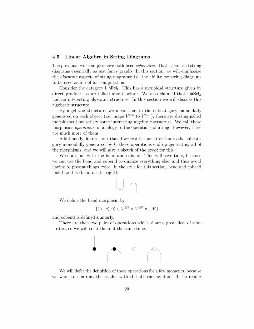
We start out with the bend and cobend. This will save time, becausewe can use the bend and cobend to dualize everything else, and thus avoidhaving to present things twice. In the style for this section, bend and cobendlook like this (bend on the right):

We define the bend morphism by

{((v, v), 0) ∈ V ⊕2 × V ⊕0|v ∈ V }

and cobend is defined similarly.There are then two pairs of operations which share a great deal of simi-

larities, so we will treat them at the same time.

We will defer the definition of these operations for a few moments, becausewe want to confront the reader with the abstract syntax. If the reader

20

prefers concrete definitions, they are advised to skip the next page, read thedefinitions, and come back.

Each of the operations can be dualized, and we write the dualized formin the following manner. If the reader imagines that the strings can be pulledand bent, then the dualization should seem (pictorially) very natural: we arejust spinning around the operations.

= =

This dualization should be defined by R ⊆ V ⊕n ⊕ V ⊕m mapsto Rop ⊆V ⊕m⊕V ⊕n by just applying (v, w) 7→ (w, v). However, it is not immediatelyclear how this dualization corresponds to the dualization via bend and cobend.The reader should attempt to work out for themselves this correspondencebefore moving on.

Each of the “forks” are commutative, that is

=

and each pair satisfies an “identity” law:

=

More generally, each of the pairs satisfy the laws for a Frobenius algebra,which are given in [FS19, §6.3]. However, rather than getting too boggeddown in all of the algebraic details, we now give concrete definitions in the

21

category LinRelk and encourage the reader to come up with his or her ownlaws that the operations satisfy.

The black dot operations are named zero:

{(0, 0) ∈ V ⊕0 ⊕ V ⊕1}

and sum{((x, y), z) ∈ V ⊕2 ⊕ V ⊕1 | x+ y = z}

The motivated reader will check that each of the properties that we haveclaimed to hold do in fact hold for this definition.

The white dot operations are named free

{(0, x) ∈ V ⊕0 ⊕ V ⊕1}

and coclone{((x, x), x) ∈ V ⊕2 ⊕ V ⊕1}

Again, the reader is invited to verify the properties that we have stated.In addition, the reader should work out the meaning of the following diagrambefore moving forward.

The last operation we need is called ratio, and is defined for [a : b] ∈ kP 1

(1-dimensional projective space over k). The definition is

{(x, y) ∈ V ⊕1 ⊕ V ⊕1 | ay = bx}

and the operation looks like.

[a:b]

Note that we can now generate all relations between k and k. Allof the one-dimensional relations are handled by ratio, and the zero and

22

two-dimensionsional relations are handled by the following two diagrams,respectively.

We will now sketch the proof that all linear relations between kn = k⊕n

and km = k⊕m are generated by these operations. We prove this with asequence of lemmas, working backwards from the conclusion. One thing thatwe should note before starting, however, is that the key thing to realize isthat what we will be doing is making a presentation of a relation. Therefore,it will not be unique, and will involve matrices.

Lemma 1. Any linear relation R ⊆ kn ⊕ km can be written as

x R y ⇔ there exists w ∈ k` such that Aw = x and Bw = y

for some fixed k`, and some fixed matrices A and B. More strongly: if{(w,Aw) | w ∈ k`} and {(w,Bw) | w ∈ k`} are relations written in terms ofthe basic operations, then we can write R in terms of the basic relations.

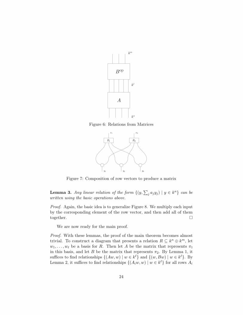
Proof. Fix a basis for R, and let k` ∼= R be the identification correspondingto that basis. Then let A be a matrix representing π1 and let B be a matrixrepresenting π2. To see the stronger claim, observe Figure 6.

The problem now reduces to showing that we can generate the relationship{(v,Av)|v ∈ kn} ⊆ kn ⊕ km for any n×m matrix A.

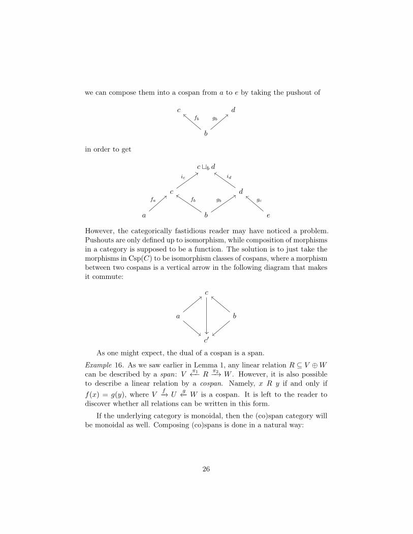
Lemma 2. Suppose that for i = 1, . . . , n, we have written the relationRi ⊆ k ⊕ km using our collection of basic operators. Then we can write therelation R ⊆ kn ⊕ km, which is defined by

x R y ⇔ xi Ri y for all i

using our collection of basic operators.

Proof. The basic idea is to generalize Figure 7. Essentially, we use the /clone/operation to split the input up into n different copies. We then apply Ri toeach of those copies.

23

A

Bop

km

k`

kn

Figure 6: Relations from Matrices

R1 R2

x1 x2

y1 y2 y3

Figure 7: Composition of row vectors to produce a matrix

Lemma 3. Any linear relation of the form {(y,∑

j ajyj) | y ∈ kn} can bewritten using the basic operations above.

Proof. Again, the basic idea is to generalize Figure 8. We multiply each inputby the corresponding element of the row vector, and then add all of themtogether.

We are now ready for the main proof.

Proof. With these lemmas, the proof of the main theorem becomes almosttrivial. To construct a diagram that presents a relation R ⊆ kn ⊕ km, letw1, . . . , w` be a basis for R. Then let A be the matrix that represents π1in this basis, and let B be the matrix that represents π2. By Lemma 1, itsuffices to find relationships {(Aw,w) | w ∈ k`} and {(w,Bw) | w ∈ k`}. ByLemma 2, it suffices to find relationships {(Aiw,w) | w ∈ k`} for all rows Ai

24

[1:a1]

[1:a2]

[1:a3]

y1 y2 y3

x

Figure 8: Creation of a row vector

of A, and {(w,Biw) | w ∈ k`} for all rows Bi of B. Finally, we can do thisby Lemma 3.

5 Cospans

5.1 Basic Cospans

Let C be a category with pushouts. Then we define a category Csp(C) inthe following way. The objects of Csp(C) are just the objects of C. However,an arrow between a, b ∈ Csp(C) is a diagram in C of the form

c

a b

fa fb

This is called a cospan.5 We also write a cospan inline like this: a fa−→ cfb←− b.

Now, if we have two cospans that share a common “foot”, i.e.

c d

a b e

fa fb gb gc

5A diagram of the formc

a b

fa fb

is called a span.

25

we can compose them into a cospan from a to e by taking the pushout of

c d

b

fb gb

in order to get

c tb d

c d

a b e

ic id

fa fb gb gc

However, the categorically fastidious reader may have noticed a problem.Pushouts are only defined up to isomorphism, while composition of morphismsin a category is supposed to be a function. The solution is to just take themorphisms in Csp(C) to be isomorphism classes of cospans, where a morphismbetween two cospans is a vertical arrow in the following diagram that makesit commute:

c

a b

c′

As one might expect, the dual of a cospan is a span.

Example 16. As we saw earlier in Lemma 1, any linear relation R ⊆ V ⊕Wcan be described by a span: V π1←− R

π2−→ W . However, it is also possibleto describe a linear relation by a cospan. Namely, x R y if and only iff(x) = g(y), where V f−→ U

g←− W is a cospan. It is left to the reader todiscover whether all relations can be written in this form.

If the underlying category is monoidal, then the (co)span category willbe monoidal as well. Composing (co)spans is done in a natural way:

26

A C B

⊗ = A⊗X C ⊗ Z B ⊗ Y

X Z Y

Example 17. The category of (possibly decorated) graphs has pushouts, sowe can form the category of cospans over this category. This category allowsus to glue together graphs along common subgraphs. Moreover, it inherits amonoidal structure from the monoidal structure on the category of decoratedgraphs.

From a purely theoretical standpoint, there is nothing wrong with theprevious example. However, if we want to model electronic circuits, in physicalpractice we only glue (or rather, solder) together terminals. It does not makesense to identify two resistors. In order to solve this issue, we need a moreadvanced framework.

5.2 Structured Cospans

One problem with cospans is that we often want to restrict the type of feet.For instance, in the case of electronic circuits, the apex of the cospan can bevery complicated: it can be a highly decorated graph. However, we want thefeet to act like “plugs”, so the feet should be discrete graphs.

The naive way to achieve this is to say that only a subset of the objectsof a category can be feet. However, this is not very categorical. A better wayis to have a “category of feet” D, along with a functor F : D −→ C. Then a“structured cospan” is a diagram of the form

c

F (a) F (b)

fa fb

Just as we can do with regular cospans, we can construct a categoryF Csp(C), where ob(F Csp(C)) = ob(D) and morphisms are isomorphismclasses of decorated cospans. This construction is due to [BC20]. Previously,there was another way of doing a similar thing called decorated cospans; itis our opinion that structured cospans are more straightforward and elegant

27

Figure 9: An Open Circuit

way of presenting many of the categories that decorated cospans were usedfor.

If D and C are monoidal categories and F is a monoidal functor, thenF Csp(C) inherits a monoidal structure in the same way that Csp(C) does,

F (a) c F (b)

⊗ = F (a⊗ x) c⊗ z F (b⊗ y)

F (x) z F (y)

5.3 Categories of Open Systems

Using the technology of structured cospans, we can efficiently describe cate-gories of open systems.

Example 18. In the section on electronic circuits, we deferred the discussionof how to construct the underlying category. We are now ready to give amore thorough treatment of this. Let F be the functor from FinSet to thecategory of R≥0-decorated graphs, Grph.

Then F Csp(Grph) is a monoidal category. A morphism in this categoryis a circuit comprised of resistors along with an assignment of “input” and“output” ports. This is pictured in Figure 9. Note that unlike our previousconvention, we draw this horizontally. This is for two reasons. One is that itfits better on the page. The other is that it is often drawn horizontally inthe literature, and we would like to accustom the reader to reading stringdiagrams horizontally as well as vertically.

Example 19. We can also construct a category of open Petri nets. There is afunctor from FinSet to Petri which sends a finite set to the Petri net with that

28

set of species and no reactions. Taking the structured cospan category onthis functor leads to a category where we can compose (isomorphism classesof) Petri nets. [BC20].

5.4 Corelations

In the next big section, we will take these structured cospan categories anddevelop semantics for them. However, this review would be incomplete if itdid not mention the theory of corelations. The essential idea of corelationsis that if all we care about in a (structured) cospan is the relationship thatit induces on the feet (as we saw before, a cospan of vector spaces inducesa linear relation on the feet), then often there are “inessential” parts of theapex of the cospan that we can discard. For instance, if we have an opencircuit, then connected components that are not connected to the input oroutput we should be able to do without. Corelations give a way of finding a“minimal” cospan that represents the same relationship as a given cospan.

We will not develop the theory here, because we do not need it for latersections, but the interested reader should refer to [Fon16].

6 Semantic Functors

One of the reasons that we are interested in open processes is so that largeunwieldy closed models can be broken up into smaller closed pieces andstudied. However, we need some sort of guarantee that after we break up thelarge unwieldy model, study the pieces separately, and put the pieces backtogether, we will have the same picture.

This guarantee comes in the form of functorial semantics. The idea isthat there are two categories, S and B. S is the category of schematics : thearrows and morphisms are descriptions for models. Then B is the categoryof behaviors: the arrows and morphisms are the actual fleshed-out model.

Then the functor assigns a semantic to each model, and the functor lawsensure that this assigning of semantics respects composition of models.

From a mathematical standpoint, there is nothing special about semanticfunctors. The interest in semantic functors comes from taking a semanticthat already exists for a certain type of model, and realizing that it is in facta functor; i.e. that the semantic respects composition.

In this section, we will discuss several semantics for the models that wehave been talking about, and show that these semantics are functorial.

29

6.1 Steady State Solutions for Resistor Networks

Suppose thatR≥0 W Jρ

s

t

is a decorated graph, which we will call C. The intent is for C to represent asimple electronic circuit. W is the set of “wires”, J is the set of “junctions”,and ρ(w) is the “inverse resistance” associated to each wire.

We are interested in steady-state (i.e., not time-varying) assignments ofvoltages to each junction that satisfy some laws from physics.

Definition 1. If {Vi}i∈J ∈ RJ is an assignment of a voltage to each circuitjunction in C, then the current flowing through a wire w : i −→ j is definedto be ρ(w)(Vj − Vi). In the real world, this is called Ohm’s law (typicallyformulated as V = IR); here it is just the definition of current.

In the real world, current is the rate at which charge flows. This isimportant, because it means that in order for charge to be conserved, thecurrent flowing into any junction must be equal to the current flowing out ofthat junction.

Definition 2. Wires in the real world are undirected. Therefore, our dec-orated graph has extraneous information. To simplify matters, we will saythat w : i↔ j if w : i −→ j or w : i←− j.

Definition 3. We say that the current incident on a junction i is

Ii =∑j∈J

∑w : i↔j

ρ(w)(Vj − Vi)

If Ii is positive, then current is coming into i and leaking out of the circuitsomehow. We say that current is conserved at i if Ii = 0.

Notice that this equation is linear in {Vi}i∈J . The set of solutions to thisequation is therefore a real vector space.

Now, in a closed system, we would require Ii = 0 for all i ∈ J . However,this does not lead to anything interesting, because it turns out that eachconnected component of the graph would have to have the same voltage inall of its junctions in order to satisfy the current conservation laws. Thus,the solution set is a vector space with dimension equal to the number ofconnected components.

In order to get interesting behavior out of a circuit, we have to add nodeswhere current can flow in and out, that is nodes where Ii 6= 0. This is always

30

the case in the real world: a circuit has (at least) a power supply, whichis held at a constant high voltage, and a ground wire, which is held at aconstant low voltage. Conservation of current does not apply at the powersupply junction or at the grounding junction.

To model this, we return to the structured cospan category for decoratedgraphs over FinSet. Consider a structured cospan

C

F (A) F (B)

f g

Then we say that a node is an external node if it lies in the image of f org, and an internal node otherwise.

We assign to this structured cospan a span in VecR, which looks like

VA,B(C)

V(A) V(B)

V(f) V(g)

VA,B(C) is the vector space corresponding to all assignments of voltagesto the junctions in C that satisfy charge conservation at internal nodes. Thatis, if {Vi}i∈J ∈ VA,B(C), then Ii = 0 for all internal i ∈ J .V(A) is RA ×RA, and V(B) is RB ×RB . V(f) and V(g) are defined by

V(f)({Vi}i∈J) = {Vf(a)}a∈A × {−If(a)}a∈AV(g)({Vi}i∈J) = {Vg(a)}a∈A × {Ig(a)}a∈A

Intuitively, V(f) sends a voltage assignment to the voltages and “input”currents of the “input” (F (A) −→ C) and V(g) sends a voltage assignment tothe voltages and “output” currents of the “output” (C ←− F (B)).

So that we don’t “double-count” current outputs, we require that f and gare injective and have disjoint images. It can be verified that this requirementleads to a subcategory of the cospan category.

The upshot of this is that when we compose spans using pullback, matchingup currents and voltages ensures that current is conserved in what is now anew internal node.

6.2 Open Dynamical Systems

In order to apply a similar semantic functor to the category of Petri nets, wewill take a brief diversion to discuss what the codomain looks like.

31

What is a dynamical system? For the sake of this thesis, we will thinkabout a dynamical system as a functor E from the category BM (the categoryrepresenting a linearly ordered commutative monoid M) into some othercategory. For instance, in physics, M is R≥0 and the “other category” isoften the category of manifolds and smooth functions. This gives a smooth“evolution” operator Et : X −→ X for each t such that Et ◦ Et′ = Et′+t.

One way of deriving such a functor is by defining a vector field (i.e.a section of the tangent bundle) on X and letting Et be the 1-parameterdiffeomorphism group associated with that vector field. This will not alwayswork, for instance if the vector field is not well-behaved. However, for thepurposes of this exposition, we will not worry about such details. We canget away with this by only considering algebraic vector fields on Rn (i.e., apolynomial map Rn −→ R

n); these are known to be sufficiently well-behavedfor our purposes. Therefore, it suffices to define a dynamical system as analgebraic vector field on Rn.

But what is an open dynamical system? In the introduction, we definedan open system as one which receives influence through its boundary. So weneed to designate a boundary, and we need to define how the open systemreceives influence through this boundary.

Designating a boundary at this point is routine: if the system is S (i.e.we will put a differential equation on RS), then a boundary is a map of setsB −→ S. Before we define how the system is affected through B, we willallows ourselves some philosophy.

Intuitively, differential equations in dynamical systems enforce conserva-tion laws. Famously, Newton’s laws conserve mass, energy, and momentum;Maxwell’s laws conserve charge and energy. When we allow these differentialequations not to hold, we are allowing conserved quantities to flow in andout of our system. Therefore, material flowing through the boundary isrepresented by a deviation from the differential equation. We express this de-viation by defining a function D : R≥0 −→ R

B , and making a new differentialequation

∂

∂ty(t) = A(y(t)) + d∗(D(t))

where d∗(D(t)) is the pushforward of v along d, defined by d∗(v)j =∑

d(i)=j vj ∈RS . D represents flows of material or energy through the boundary B.

Example 20. In an electrodynamical system, D(t) could represent the currentflowing through the boundary at time t.

Example 21. In a thermodynamical system where y0, y1 are the temperatureand pressure of the environment, then we might assert through fiat that

32

y0(t) = C0 and y1(t) = C1 for all time, and exempt them from being affectedby the system. This would result in heat transfers and volume or moleculetransfers through the boundary of the system, and we could capture this bymaking Di(t) = −Ai(y(t)), so that ∂

∂t yi(t) = 0.

We want to make a category of open dynamical systems. In order to dothis, we need to split the boundary into input and output components, sothat we have a cospan.

S

X Y

io

Then, given I : R≥0 −→ RX and O : R≥0 −→ R

Y , we define the equationassociated to an open dynamical system to be:

∂

∂tx(t) = A(x(t)) + i∗(I(t))− o∗(O(t))

i∗ and o∗ are the pushforward maps, which are defined by:

i∗(v)k =∑i(j)=k

vj

o∗(v)k =∑o(j)=k

vk

Finally, to compose two open dynamical systems

S1 S2

X1 Y1 = X2 Y2

i1o1

i2o2

with vector fields A1 : RS1 −→ RS1 and A2 : RS2 −→ R

S2 , we take the pushout

S = S1 tY1=X2 S2

S1 S2

X1 Y1 = X2 Y2

i1o1

i2

o2

33

and associate with it a vector field A : RS −→ RS defined by A(v) = A1(v|S1)+

A2(v|S2).That this construction ends up making a well-defined category is proved

in [Pol17].The way that we suggest thinking about the category of open dynamical

systems is that when we fix flows on the boundary, we end up being ableto evolve the state of the system through time. As we suggested in theintroduction, a good way to do this is by defining a functor from the posetR to the category of manifolds, so that we have a smooth map from R

n toRn for every poset morphism t −→ t′. The mechanism of the algebraic vector

field is a somewhat arbitrary implementation of this, which we put in placebecause it guarantees good behavior.

6.3 Rate Equation for Petri Nets

Our motivation for introducing the category of open dynamical systems was togive a semantic for Petri nets. By what we said above, it suffices to associatea differential equation to each Petri net (or more formally, an algebraic vectorfield). Once we have done this, a structured cospan F (a) −→ c←− F (b) withfeet finite sets, and with apex a Petri net, will map to an open dynamicalsystem in a natural way.

We derive the form of this differential equation through three principles[BB12]. But before we get into the derivation, we make one clarifying remark.Previously, we associated to each reaction a rate. However, we would nowlike to use “rate” to refer to the speed at which the reaction is taking placeat an instant in time. Therefore, we will use the term “rate multiplier” torefer to the earlier “rate”, and reserve the term “rate” for instantaneous rate.

With that cleared up, here are the three principles.

1. The rate of a reaction only depends on the current concentrations ofspecies, not on the rate of any other reaction.

2. The rate of a reaction is proportional to the product of the currentquantities of the inputs, multiplied by the base rate.

3. The derivative of species concentration in a single-reaction Petri netis proportional to the difference between the number of that speciesproduced and consumed by that reaction, multiplied by the rate of thatreaction.

These principles have the following consequences.

34

s

Figure 10: Exponential Decay

1. A = A1 + . . .+Ak, where Ai is the operator associated to a Petri netwith only reaction i. Therefore, we assume that k = 1, and we let r bethe rate associated to the single reaction, ni be the number of species ioutput by the reaction and mi be the number of species i consumed bythe reaction.

2. If yi = Et(x0)i, then the rate of the one reaction is r∏i ymii .

3. The jth component of A(y) is (nj −mj)r∏i ymii .

The differential equation that we end up with after applying these princi-ples is called the rate equation. It is possible to write down the rate equationin a closed form, but it is our opinion that no clarity is gained from that.Instead, we will do examples.

Example 22. Suppose that we are tasked to model the behavior of a lump ofuranium. Famously, uranium randomly decays into other particles (whichwe don’t care about). We model this with a Petri net with one species,uranium, and one reaction, decay, which has input a single molecule ofuranium, and output nothing. The schematic for this is in Figure 10. Weonly have one species and one reaction, and m0 = 1 while n0 = 0. Therefore,A(y) = (0− 1)ry1 = −ry. This is the well-known equation for exponentialdecay, with solution yt = y0e

−rt. Therefore, Et = e−rt. It is rare that thereis a closed form solution for Et, except for in simple cases like this one.

Example 23. Recall the Petri net presented in Figure 2. Let rB, rP and rDbe the rate multipliers associated to “birth”, “predation”, and “death”, and letyR be the concentration of rabbits while yW is the concentration of wolves.Then the rate of birth is rByR, the rate of predation is rP yRyW , and the rateof death is rDyW . The resulting system of differential equations is

∂

∂tyR = rByR − rP yRyW

∂

∂tyW = rP yRyW − rDyW

There is not a corresponding closed form solution for the evolution operator,however this can be evaluated numerically.

35

The author has created a tool for numerical solutions of the rate equation,which is available online at https://owenlynch.org/static/ez-petri. Nodownload is required: it runs in the browser. The source code is also freelyavailable at https://github.com/olynch/ez-petri.

Now that we have defined the rate equation, we can define a functor fromthe category of open Petri nets to the category of open dynamical systems.This functor is more or less straightforward: we send an open Petri net

P

F (X) F (Y )

to a open dynamical system with underlying cospan

S

X Y

where S is the set of species in P , along with the rate equation on S.

36

References

[BB12] John C. Baez and Jacob Biamonte.Quantum Techniques for Stochas-tic Mechanics. 2012. arXiv: 1209.3632v5 [quant-ph].

[BC18] John C. Baez and Kenny Courser. “Coarse-Graining Open MarkovProcesses.” In: (Nov. 21, 2018). arXiv: 1710.11343 [math-ph]. url:http://arxiv.org/abs/1710.11343 (visited on 03/05/2020).

[BC20] John C. Baez and Kenny Courser. “Structured Cospans.” In: (Jan. 3,2020). arXiv: 1911.04630 [math]. url: http://arxiv.org/abs/1911.04630 (visited on 04/13/2020).

[BS09] John C. Baez and Mike Stay. “Physics, Topology, Logic and Compu-tation: A Rosetta Stone.” In: (2009). arXiv: 0903.0340v3 [quant-ph].

[Fon16] Brendan Fong. “The Algebra of Open and Interconnected Systems.”In: (Sept. 17, 2016). arXiv: 1609.05382 [math]. url: http://arxiv.org/abs/1609.05382 (visited on 04/13/2020).

[FS19] Brendan Fong and David I. Spivak. An Invitation to Applied Cat-egory Theory: Seven Sketches in Compositionality. 1st ed. Cam-bridge University Press, July 18, 2019. isbn: 978-1-108-66880-4 978-1-108-48229-5 978-1-108-71182-1. doi: 10.1017/9781108668804.url: https://www.cambridge.org/core/product/identifier/9781108668804/type/book (visited on 04/13/2020).

[Lei03] Tom Leinster. “Higher Operads, Higher Categories.” In: (May 2,2003). arXiv: math/0305049. url: http://arxiv.org/abs/math/0305049 (visited on 04/23/2020).

[Pol17] Blake S. Pollard. “Open Markov Processes and Reaction Networks.”In: (Sept. 29, 2017). arXiv: 1709.09743 [cond-mat, physics:math-ph].url: http://arxiv.org/abs/1709.09743 (visited on 04/13/2020).

[Sch81] J. Schnakenberg. Thermodynamic Network Analysis of BiologicalSystems. Universitext. Berlin, Heidelberg: Springer Berlin Heidel-berg, 1981. isbn: 978-3-540-10612-8 978-3-642-67971-1. doi: 10.1007/978-3-642-67971-1. url: http://link.springer.com/10.1007/978-3-642-67971-1 (visited on 04/13/2020).

37