operational intelligence for advanced process and...

Presented by

© Copyright 2013 OSIsoft, LLC.

Operational Intelligence for advanced process and asset monitoring

Luis Yacher, CONTAC

© Copyright 2013 OSIsoft, LLC. 2

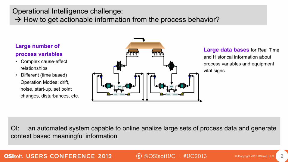
Operational Intelligence challenge: à How to get actionable information from the process behavior?

Large number of process variables •  Complex cause-effect

relationships •  Different (time based)

Operation Modes: drift, noise, start-up, set point changes, disturbances, etc.

Large data bases for Real Time and Historical information about process variables and equipment vital signs.

OI: an automated system capable to online analize large sets of process data and generate context based meaningful information


Operational Intelligence challenge: à How to get actionable information from the process behavior?

•  How to determine early alerts if the process or equipment is deviating from a pattern or moving to a new one, being an “on quality pattern”, a “throughput pattern”, an “efficiency patter”, a “malfunction pattern”, etc.?

•  How to determine the “most influencing” factors that drives the evolution of a certain process variable or equipment vital sign KPI?

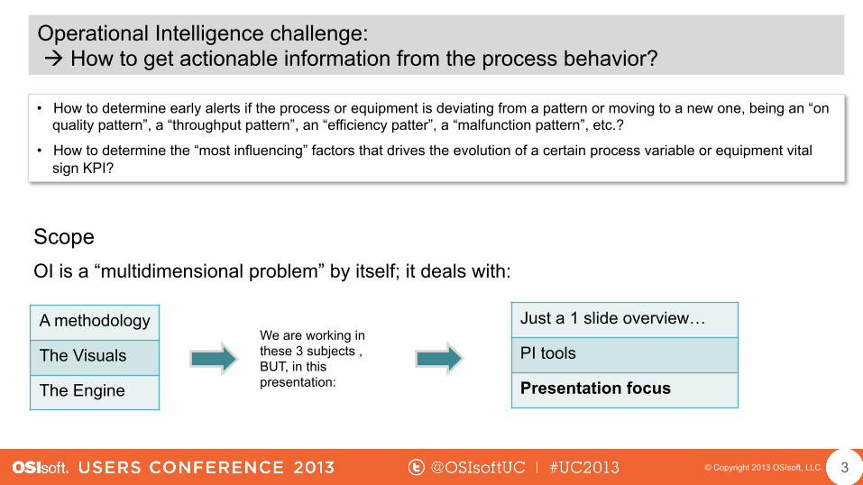
Scope

OI is a “multidimensional problem” by itself; it deals with:

We are working in these 3 subjects , BUT, in this presentation:

A methodology

The Visuals

The Engine

Just a 1 slide overview…

PI tools

Presentation focus


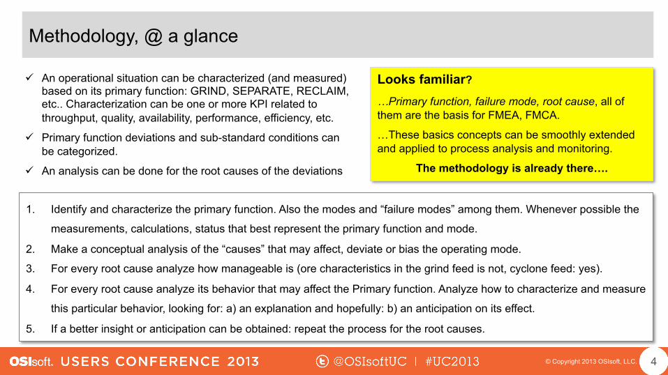
Methodology, @ a glance

ü  An operational situation can be characterized (and measured) based on its primary function: GRIND, SEPARATE, RECLAIM, etc.. Characterization can be one or more KPI related to throughput, quality, availability, performance, efficiency, etc.

ü  Primary function deviations and sub-standard conditions can be categorized.

ü  An analysis can be done for the root causes of the deviations

Looks familiar?

…Primary function, failure mode, root cause, all of them are the basis for FMEA, FMCA.

…These basics concepts can be smoothly extended and applied to process analysis and monitoring.

The methodology is already there….

1.  Identify and characterize the primary function. Also the modes and “failure modes” among them. Whenever possible the

measurements, calculations, status that best represent the primary function and mode.

2.  Make a conceptual analysis of the “causes” that may affect, deviate or bias the operating mode.

3.  For every root cause analyze how manageable is (ore characteristics in the grind feed is not, cyclone feed: yes).

4.  For every root cause analyze its behavior that may affect the Primary function. Analyze how to characterize and measure

this particular behavior, looking for: a) an explanation and hopefully: b) an anticipation on its effect.

5.  If a better insight or anticipation can be obtained: repeat the process for the root causes.

4


Throughput and quality KPI

Classification

Cyclone status Density Control Grinding

Perfomance Pressure Control

Other Ore feed size distribution

•  For every behavior (Causes and Effects), a specific RtKPI is selected.

•  RtKPI are structured and managed in PI-AF

•  Model implementation: a context based representation of the cause & effect

relationships and its related measurements,

Methodology, @ a glance

•  The C-E model being managed in PI-AF.

•  A set of templates for the calculation libraries that runs on PI-ACE.


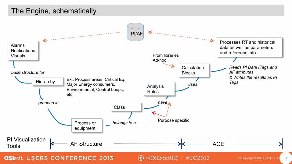
The Engine

ü  The OI Model Runs in PI-AF, calculation block in PI-ACE

ü  OI model defines •  The process or equipment decomposition tree for the C-E modeling •  At any level the RtKPI evaluation blocks are assigned •  Tree hierarchy can be used in case of roll-up KPI calculations

ü  The OI model is purpose specific, ex.: operational performance, equipment monitoring, energy efficiency, environmental, early alert of malfunctions, critical condition evaluation, variability monitoring, control loop assessment (*).

ü  There are two “calculation blocks families”: single variable and

multivariable.

ü  The overall architecture allows for the inclusion of specialized

calculation blocks

ü  OI model “reads” data from PI Tag´s and “writes” RtKPI as PI Tag´s.

Visualization is made using the standard PI tools, as well as the related

ones, such as PowerPivot or similar.

(*) A dedicated set of KPI libraries is available for this purpose


The Engine, schematically

Process or equipment

Alarms Notifications Visuals

Class

Hierarchy Analysis Rules

have

Calculation Blocks

Processes RT and historical data as well as parameters and reference info

uses

Reads PI Data (Tags and AF attributes & Writes the results as PI Tags

grouped in

base structure for

AF Structure ACE PI Visualization Tools

Ex.: Process areas, Critical Eq., Major Energy consumers, Environmental, Control Loops, etc.

Purpose specific

From libraries Ad-hoc

belongs to a

PI/AF


The Engine, calculation blocks and methods

Single Variable Description

Harris Evaluates error variance

IAE (ITAE, ISE, ITSE) Absolute error total (integral)

Miao Seborg Oscilation index based on auto covariance.

Forsman Statting Oscilation index. Computes the areas whenever the variable is crossing “zero”

D3 Scheffe’s test, detect behaviour changes.

Time on state State histograms

Distributión Time on range, for selected ranges

General Statistics As available in PI AF

Mostly used for control loop monitoring

Multi Variable Description Purpose

VFA Variability Factor, evaluate the most influencing factors for a specific behavior. Process analysis- Data Mining

PLS On line estimation of selected variables. Process Modeling

SBM Similarity based Method; evaluates if the current behavior corresponds to a recorded pattern. Also a self learning method for new patterns

Variability indexes

8


Date selection

Controller selection

Variable values distribution histogram

IAE Trend

Forsman Index

(Oscillations)

Miao Seborg Index (Osc,)

Controller state statistics

The Engine, calculation blocks and methods, app. Example, single variable RtKPI

PB Visualization of RT calculation blocks results. Example: Control loop monitoring


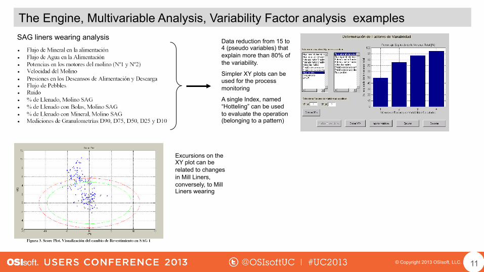
The Engine, Multivariable Analysis, Variability Factor analysis

From “n” process variables, generate a set of “m” new variables or “Variability Factors” that: •  m < < n (reduction in the complexity of the interpretation) •  The VF´s are expressed as a linear function of the original “n” variables (linear on the parameters, the

variables can be preprocessed, ex.: squared, log, etc.) •  The VF´s are selected as those that explains “most” of the variability of the original “n”.

THEN The process behavior can be characterized using the reduced set of new variables, specifically: using statistical indexes to evaluate patterns. USES •  Deviation from a pattern can be related to a process sub-standard condition or equipment failure. •  Belonging to a pattern can provide an insight about the most influencing factors at a certain time.

•  A new generation of “process visualization” for operator empowering, beyond trends.


The Engine, Multivariable Analysis, Variability Factor analysis examples SAG liners wearing analysis Data reduction from 15 to

4 (pseudo variables) that explain more than 80% of the variability.

Simpler XY plots can be used for the process monitoring

A single Index, named “Hotteling” can be used to evaluate the operation (belonging to a pattern)

Excursions on the XY plot can be related to changes in Mill Liners, conversely, to Mill Liners wearing

11


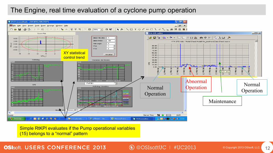
A model was built for the centrifugal pumps (many).

Model represents “normal operating conditions.

Deviation from the pattern is measured by two Indexes T2 and SPE.

Simple RtKPI evaluates if the Pump operational variables (15) belongs to a “normal” pattern

Normal Operation

Abnormal Operation Normal

Operation

Maintenance

The Engine, real time evaluation of a cyclone pump operation

XY statistical control trend

12


The Engine, Process and Equipment Modeling, the PLS technique

VFA XY Plot

Using the historical data a VFA analysis was done, being the goal to determine a pattern model for the SAG mil operation as well as the relationship of the Pattern visualization with the process variables


The Engine, Process and Equipment Modeling, the PLS technique

For a set of “X” input variables and “Y” output variables, applying similar statistical technics as described, it is possible to determine a reduced set of variables that: •  represents the variability of the original ones •  with a much les quantity of variables •  AND: are “orthogonal” or “independent” variables

•  Then a model can be developed, that calculates the relationship of the “new” set of I/O. And using the “reduction” equations, the model that relates the original X and Y variables.

USES •  Evaluate difficult to measure process variables, ex.: when the “Y” can be measured by offline sampling and analysis only.

•  Similar, but using the model to provide information between lab analysis

•  Compare the actual operation against selected behavior models.

•  Run the model online, if the output fits the actual operation, it is reasonable to infer that the influencing factors of the model are representative of the real operation. This provides actionable information for the operator

14


For each SAG mil a model was developed. Based in a pattern analysis of the history, a model was built that correlates the “max throughput” with the current one, using Mill variables and Size distribution variables. Also shows: The individual weighing factors of the Key operational variables, as related to the throughput. A set of XY plots with an indication of the preferred operating zone. Also shows the “ROC” or rate of change of selected variables. The goal of this application was to empower the operator by a new type of process visualization, giving a deeper insight about what to do and the consequences of its actions.

The Engine, Process and Equipment Modeling, the PLS technique example.


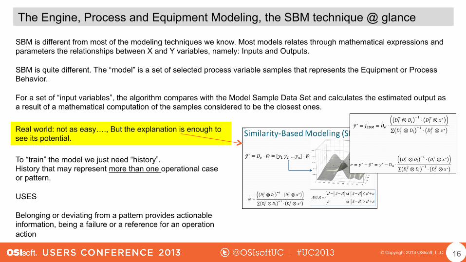
The Engine, Process and Equipment Modeling, the SBM technique @ glance

SBM is different from most of the modeling techniques we know. Most models relates through mathematical expressions and parameters the relationships between X and Y variables, namely: Inputs and Outputs. SBM is quite different. The “model” is a set of selected process variable samples that represents the Equipment or Process Behavior. For a set of “input variables”, the algorithm compares with the Model Sample Data Set and calculates the estimated output as a result of a mathematical computation of the samples considered to be the closest ones.

Real world: not as easy…., But the explanation is enough to see its potential.

To “train” the model we just need “history”. History that may represent more than one operational case or pattern. USES Belonging or deviating from a pattern provides actionable information, being a failure or a reference for an operation action

16


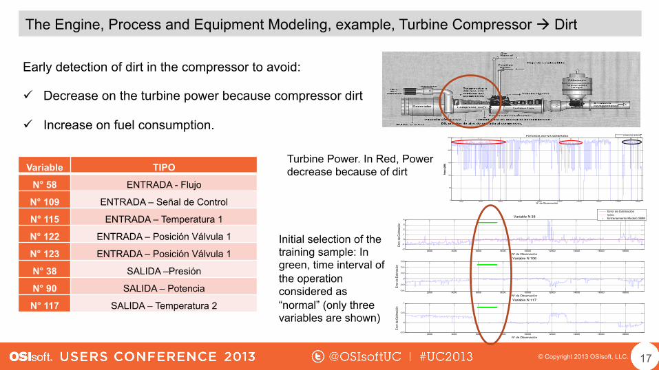
The Engine, Process and Equipment Modeling, example, Turbine Compressor à Dirt

Early detection of dirt in the compressor to avoid:

ü  Decrease on the turbine power because compressor dirt

ü  Increase on fuel consumption.

Variable TIPO

N° 58 ENTRADA - Flujo

N° 109 ENTRADA – Señal de Control

N° 115 ENTRADA – Temperatura 1

N° 122 ENTRADA – Posición Válvula 1

N° 123 ENTRADA – Posición Válvula 1

N° 38 SALIDA –Presión

N° 90 SALIDA – Potencia

N° 117 SALIDA – Temperatura 2

1000 3000 5000 7000 9000 11000 13000 15000 17000 190000

50

100

150

200

250

N° de Observación

Poten

cia [M

W]

POTENCIA ACTIVA GENERADA

Potencia Activa

21 3

Turbine Power. In Red, Power decrease because of dirt

2000 4000 6000 8000 10000 12000 14000 16000 18000-2

-1

0

1

2

3

4Variable N 38

N° de Observación

Erro

r de E

stima

ción

Error de EstimaciónCeroEntrenamiento Modelo SBM

2000 4000 6000 8000 10000 12000 14000 16000 18000-0.4

-0.2

0

0.2

0.4

0.6Variable N 106

N° de Observación

Erro

r de E

stima

ción

2000 4000 6000 8000 10000 12000 14000 16000 18000-0.5

0

0.5

1Variable N 117

N° de Observación

Erro

r de E

stima

ción

Initial selection of the training sample: In green, time interval of the operation considered as “normal” (only three variables are shown)

17


Final Remarks

Process and equipment history can be processed and structured towards the identification of patterns and cause-effect relationships. Patterns and relationships can empower both, analysts and operators, providing a deeper insight of the process and equipment behavior, early alert of deviations or failures as well as the consequences of its actions. AND All of this can be implemented using the PI-AF-ACE infrastructure, in an modular, comprehensive and manageable manner. Modeling tools and online deployment framework exists. Not needing to be an expert mathematician, just have a deep knowledge about the process.

18


Luis Yacher S [email protected] Manager CONTAC www.contac-scan.com

19

Brought to you by


operational intelligence for advanced process and...

Documents