operational space control of a c the author(s) 2017...

Operational space control of a

lightweight robotic arm actuated by

Shape Memory Alloy wires: a

comparative study

Journal TitleXX(X):1–18c©The Author(s) 2017Reprints and permission:sagepub.co.uk/journalsPermissions.navDOI: 10.1177/ToBeAssignedwww.sagepub.com/

Serket Quintanar-Guzman, Somasundar Kannan, Adriana Aguilera-Gonzalez, Miguel A.

Olivares-Mendez and Holger Voos

Abstract

This paper presents the design and control of a two-link lightweight robotic arm using Shape Memory Alloy wiresas actuators. Both, a single wire actuated system and an antagonistic configuration system are tested in open andclosed-loop. The mathematical model of the SMA wire, as well as the kinematics and dynamics of the robotic arm, arepresented. The Operational Space Control of the robotic arm is performed by using a Joint Space control in the innerloop and Closed Loop Inverse Kinematics in the outer loop. In order to choose the best Joint Space Control approach, acomparative study of four different control approaches (Proportional Derivative, Sliding Mode, Adaptive and AdaptiveSliding Mode Control) is carried out for the proposed model. From this comparative analysis, the adaptive controllerwas chosen to perform Operational Space Control. This control helps us to perform accurate positioning of the end-effector of SMA wire based robotic arm. The complete Operational Space control was successfully tested throughsimulation studies performing position reference tracking in the end-effector space. Through simulation studies theproposed control solution is successfully verified to control the hysteretic robotic arm.

Keywords

SMA wire, Adaptive Control, Lightweight Robotic Arm, Operational Space position control, hysteresis.

Introduction

Shape Memory Alloys (SMA) are a type of smartmaterials that can “remember” their original shapes.These type of alloys have the ability to recoverits original pre-defined shape by applying certainstimuli such as thermo-mechanical variations. Thisphenomenon is known as Shape Memory Effect(SME)(Rao et al., 2015). The SME occurs due toan inner transformation of the material’s crystallinestructure. This transformation happens between twophases called martensite and austenite. When theSMA wire is at lower temperature its structure shiftsto the martensite phase which is a relatively softand malleable phase, during which the wire can beeasily deformed. When heated over the transformationtemperature, the SMA wire transforms back into theaustenite phase, a hard phase, recovering its initialform and size (Rao et al., 2015).

Among the more common SMAs one can findfor example Nickle-Titanium, Gold-Cadmium andCopper-Zinc-Aluminium. Where the most used one

has been the Nickel-Titanium alloy (which is alsoknown as Nitinol) (Zheng et al., 2014). There areseveral physical properties of Nitinol being studiedand tested, such as: shape memory, pseudo-elasticity,corrosion resistance, magnetic susceptibility, damping,mass ratio, small size, noiseless operation, heatcapacity, bio-compatibility, thermal conductivity, andother mechanical properties including hardness, impacttoughness, fatigue strength and machinability. Theseproperties make SMA wires ideal for applicationssuch as biomedical and dental implants, aerospace,engineering and sports equipment, among others.SMAs have drawn significant attention and inte-

rest since a few decades. However, it was not until

Interdisciplinary Centre for Security, Reliability and Trust (SnT),University of Luxembourg, LU

Corresponding author:

Serket Quintanar-Guzman, SnT, University of Luxembourg,6 rue Richard Coudenhove-Kalergi , L-1359, Luxembourg, LU.

Email: [email protected]

Prepared using sagej.cls [Version: 2015/06/09 v1.01]

2 Journal Title XX(X)

recent years when the term shape memory tech-nology (SMT) was introduced and a wide rangeof SMA wires’ applications started to be deve-loped. An example of these applications is the bio-inspired micro-robots manufacturing, where SMAsare considered as a good alternative to traditionalactuators, due to characteristics as corrosion resis-tance, simple mechanical structure and biocompati-bility (Khodayari et al., 2011; Colorado et al., 2011;Gao et al., 2014; Shin et al., 2015). SMA wires havealso been used in medical devices like intra-arterialsupports (Nematzadeh and Sadrnezhaad, 2012) orwires for suturing (Nespoli et al., 2015), in orthope-dic devices as a spinal cage implant (Andani et al.,2015), adaptive anklefoot orthoses (Mataee et al.,2015) or skeletal fixation devices (mandibular seg-mental) (Moghaddam et al., 2016), as well as den-tal and orthodontic applications (Jafari et al., 2008;Pandis and Bourauel, 2010). In parallel, SMA wireshave also proved to be a good alternative when dealingwith aerodynamic problems requiring high-precisioncoordination, and some solutions have been appliedfor small prototypes and unmanned aerial vehicles(UAVs). For example in Rodrigue et al. (2016), a mor-phing segment actuated by multiple embedded SMAwires was implemented in a UAV wing, where thecapability to maintain a smooth twisting concentratedon a segment of the wing was tested with a prototype.Similarly, it is possible to include as well the work ofBarbarino et al. (2009), which presents a wing shapecontrol using SMA wires as actuation devices to pro-duce a local bump. Furthermore, Kennedy et al. (2004)presented a blade actuator that is developed for thehelicopter blade-tracking problem, which utilizes theSMA as the active actuator material to drive a rotorblade trim tab for the purpose of maintaining rotortracking. All these articles and several others proposesolutions to improve the aerodynamic properties of theflying devices.

Among the many applications of the SMAwires, several specific purpose actuators have beenreported in the literature, such as: constructionvibrations dampers (Sreekumar et al., 2009), cameralens focus actuators (Son et al., 2009), car mirroractuators (Williams et al., 2010) or SMA based motors(Quintanar-Guzman et al., 2014). Moreover, SMAwires are also useful in robotic manipulators sincethey allow motion without using larger drives. Forinstance, the human-like robotic arm developed byHulea and Caruntu (2014), where a neural networkcontrol for artificial muscles was implemented on arobotic arm joint using a SMA wire as actuator.Another example is given by Ko et al. (2011), where

the authors propose a fuzzy-PID control of ananthropomorphic artificial finger actuated by threeantagonistic SMA muscle pairs. In addition to theaforementioned, multiple general purpose actuatorshave been developed for micro-positioning applicationsusing advanced control techniques (Kannan et al.,2010, 2013; Kannan, 2011).

Nonetheless, most of the mentioned applicationsare micro-scale or require complicated mechanicalsystems to be implemented. For this reason, in aprevious publication the design of a SMA wire actuatedrobotic arm was presented (Quintanar-Guzman et al.,2016). This proposal seeks to keep the simplicity ofthe mechanics and therefore achieves a lightweightactuator capable of producing a relevant amountof force levels, leading to a suitable performanceper weight ratio. This lightweight characteristic iscritical in applications like robotic manipulators forUAVs, where the optimal use of available payloadis a great challenge. This implementation will bethe main purpose of this arm. With this in mind,we propose a suitable controller for the lightweightrobotic arm design, which enables the arm tobe implemented without significantly decreasing thequadcopter’s available payload.

This paper contains two main contributions:first, a comparative analysis between two differentconfigurations of the robotic arm is presented, in orderto study the nonlinearities of SMA wires as hysteresis,saturation and dead zone. Second, the development ofa control concept which is capable of dealing with thenonlinear dynamics of SMA wires is discussed. Alongwith slow dynamics, the nonlinear response of theSMA wire entails a huge challenge for implementationsthat require high accuracy or fast response. Forthis purpose, a comparative analysis among fourdifferent control approaches is presented: ProportionalDerivative (PD) control, Sliding Mode Control (SMC),Adaptive Control and Adaptive Sliding Mode Control(ASMC) is presented. These controllers are comparedwith the aim to find a suitable controller forthe proposed lightweight robotic arm. The selectedcontroller is then used for the development of anoperational space control for position regulation of theend-effector.

The remaining of this paper is organized asfollows: First we present the mechanical design andmathematical model of the proposed lightweightrobotic arm, followed by a comparison between thetwo different joint configurations proposed for theactuator (biased SMA wire and two antagonisticwires). Subsequently four different control approachesin joint space are developed and analysed, continued by

Prepared using sagej.cls

Quintanar-Guzman, et al. 3

a thermal disturbance analysis. After, an operationalspace control law for position regulation of the end-effector is applied. Finally we conclude with thediscussion of the results and possible future works.

Basic structure of the SMA actuated

robotic arm

In this section we present the mechanical designof a lightweight SMA actuated robot arm in twodifferent possible configurations: single biased wire andantagonistic wires.

The optimal use of available payload of an aerialvehicle is critical for the design of aerial manipulators.With this in mind, we propose a single Degree ofFreedom (DOF) actuator wich is actuated by SMAwires. In the Figure 1, a Computer Aided Design(CAD) model of the robot arm design is shown.The design is based on an existing joint proposedin Guo et al. (2015), which consists of two couplersjoined by a torsion spring. This design allows toselect between a single wire actuated system or anantagonistic configuration.

In the first configuration (biased single wire) theSMA wire is attached at one end to the coupler-1, whilethe second coupler is fixed with a hard wire, i.e., onlyone wire is a SMA wire. With this design, the actuatorbehaves like a biased SMA wire. Here, the SMA-1affects directly the angular position of the end effector(θ1) by controlling the angular position of coupler-1(see Figure 1) while the deformation force is appliedby the torsion spring and is directly proportional tothe position of coupler-1.

For the second configuration (antagonistic wires)each wire is attached at one end to its respectivecoupler, allowing to control independently the angularposition of each coupler. Controlling the secondcoupler’s position allows to adjust the torque appliedby the torsion spring and hence, increase or decreasethe overall stiffness of the joint as required. This changein stiffness entails a change in the transformationtemperatures, so the wire’s transformation could behastened in a controlled manner. The following sectionspresent a more detailed analysis of the characteristicsof these two designs.

The given robotic arm with 1 DOF, is activated bytwo 37 cm long Nitinol wires. It has two custom-madecarbon fiber links (150 mm and 100 mm respectively)and the range of movement along the vertical planeX-Z is up to 85 degrees with two 7.5 mm radiuscouplers. It has a total weight of 48 g, which is onlyabout 25% of the weight of other lightweight designsfound in the literature, such as the one presented

Figure 1. Proposed SMA wire actuated robotic arm CADmodel.

in Bellicoso et al. (2015). The winding wheels enablethe use of longer SMA wires in order to increasethe movement range without increasing the dimensionof the links. It is important to emphasize that anincrease in the length of the wires will increasethe energy consumption. For this reason a balancebetween range of motion and energy consumptionshould be considered, especially when considering amobile application like aerial manipulation.

Model of the SMA actuated robotic arm

In this section the mathematical model of the overallsystem is discussed. The mathematical model of theSMA wires, as well as the kinematics and dynamicsof the arm resulting from the mechanical design areexplained in detail.

Figure 2 shows the block diagram of the roboticarm’s mathematical model for both configurations: a)shows the single wire biased configuration, and b)the antagonistic configuration. The robotic arm modelconsist of two main subsystems: 1) the SMA wire modeland 2) the Kinematic and Dynamic model.



SMA-1model

SMA-2model

Dynamics

KinematicsSMA-1

KinematicsSMA-2

Robotic arm model (antagonistic config.)

θ1

θ2

ε1

ε2

σ1

σ2

θ1

V1

V2

(b)

SMA-1model

Dynamics

KinematicsSMA-1

Robotic arm model (biased SMA wire config.)

V1 θ1σ1

θ1ε1

(a)

Figure 2. Block diagram of the SMA actuated robotic arm,(a) biased wire configuration; (b) antagonistic configuration.

SMA wire subsystem

The schematic model describing the SMA wiresubsystem is illustrated in the Figure 3. Thissubsystem is described by a mathematical model ofthe Nitinol wire which was proposed by the authorsin Elahinia and Ashrafiuon (2002). This is likewisedivided into three subsystems representing the thermaldynamics, the heat transformation and the constitutivemodel. In the Figure 3 the interaction between thevariables of each subsystem of the SMA wire modelis shown. On the other hand, the dynamics of the armare directly derived from a CAD model. Each of thementioned subsystems will be explained in more detailin the following subsections.

Heat transfer model. This block consists of theelectrical heating (Joule effect) and the natural

Heat transfermodel

Phase trans-formationmodel

Constitutivemodel

SMA wire model

V σξT

T

σ,σ, ξ

ε

Figure 3. SMA wire mathematical model block diagram.

convection model described by the following equation(Elahinia and Ashrafiuon, 2002):

mwcpdT

dt=

V 2

R− hAw (T − Tamb) (1)

where V is the voltage, R is the electric resistanceper unit length, cp is the specific heat, mw is themass per unit length, Aw is the wire surface area,Tamb the ambient temperature and T is the SMA wiretemperature. Here h is approximated by a second orderpolynomial of the temperature:

h = h0 + h2T2 (2)

SMA wire phase transformation model. As shownin the Figure 3, the block containing the phasetransformation model (from martensite to austenite)computes the martensite fraction (ξ). The phasetransformation of the SMA wire depends directly onthe direction of the time derivative of the temperature.Therefore, due to hysteresis behavior two equationsare needed to fully describe this phenomenon. Thisphase transformation while heating is given by(Elahinia and Ashrafiuon, 2002):

ξ =ξM2

cos [aA (T −As) + bAσ] + 1 (3)

for As +σCA

≤ T ≤ Af + σCA

.

Inversely, the transformation from austenite tomartensite, during cooling is described by the followingequation (Elahinia and Ashrafiuon, 2002):

ξ =1− ξA

2cos [aM (T −MF ) + bMσ] +

1 + ξA2

(4)

for Ms +σ

CM≤ T ≤ Mf + σ

CM, where Ms, Mf , As, Af

are the start and end transformation temperaturesfor martensite and austenite transformation respec-tively. Here aA = π

(Af−As), aM = π

(Ms−Mf ), bA = − aA

CA,

bM = − aM

CM, CA and CM are curve fitting parameters.



Wire constitutive model. This model describes therelation between stress σ, strain ε, temperatureT and martensite fraction ξ. The general form,firstly proposed by Liang and Rogers (1990) and thenmodified by Elahinia and Ashrafiuon (2002), is writtenas

σ = Eε+Ωξ +ΘT , (5)

where Ω and Θ represent the phase transformationconstant and thermal expansion coefficient, respec-tively. Herein

Ω = −Eε0 (6)

and ε0 is the initial strain. The authors ofElahinia and Ashrafiuon (2002) propose a constantvalue for the Young’s modulus E as an average ofthe Young’s modulus of each phase, austenite (EA)and martensite (EM ). However, since one of theconfigurations of the actuator presented here uses theantagonistic SMA wires configuration, the Young’smodulus cannot be constant since it depends on thestress applied over each wire, which in turn depends onthe martensite fraction as follows (Guo et al., 2015):

E = ξEM + (1− ξ)EA (7)

Kinematic and dynamic model

In this section the model of the mechanical design(corresponding to the kinematic and dynamic model)and its relation with the rest of the system is explained.

Kinematic model. This model relates the SMA wiremodel with the mechanics of the robotic arm itself.The strain ratio of the SMA wire and angular velocityof the arm depends on the geometry of the design. Thiskinematic relation is given as:

ε = −rθ

l0(8)

where r is the coupler radius, l0 the initial length ofeach wire and θ the angular velocity of the coupler.Equation (8) shows that the angular position of eachcoupler with respect to the X-axis (θ) is inverselyproportional to the strain of the wire (ε).

Dynamic model. The dynamic model used heredescribes the relation between coupler mechanism,torsion spring and forces applied by the SMA wires,as well as the effects of the load and grip at the endof the second link. The general dynamic model of themechanical system is described as:

M (θ) θ + Vm

(

θ, θ)

θ + g (θ) + Fdθ +Φ(θ, θr) = τω

(9)

where θ, θ, θ represent the positions, velocities andaccelerations of the couplers, M (θ) is the inertia

matrix, Vm

(

θ, θ)

is the centripetal-coriolis matrix,

g (θ) is considered as the effect of gravity, Fd isthe viscous coefficient term, Φ (θ, θr) is the nonlinearhysteretic term, τω is the input torque applied to themanipulator joint by the SMA wire.The dynamic behavior of the couplers, gripper, load

and links was directly obtained from the CAD designshown in Figure 1 (this CAD design was developedin the Autodesk/Inventor software tool). This modeldoes not only include the exact geometry of each piecebut also masses, inertias and centers of mass necessaryfor the dynamic analysis. The CAD model is importedvia the SimMechanics toolbox in order to obtain acontinuous dynamic MATLAB/Simulink model of themechanical system. On the other hand, the torsionsprings and SMA wires torques were obtained frombasic physical laws, where the SMA wire’s force (Fw) isdeduced by inversely proportional realtion to the stress(σ), which can be computed by integration of equation(5):

τwi = Fwiri = Aσiri (10)

where i = 1, 2 for SMA-1 and SMA-2, r is the couplerradius and A is the cross-sectional area of the wire.The torsion spring torque τs for the single wireconfiguration is calculated as:

τs = ksθ1 + bsθ1 (11)

where ks is the spring constant and bs is thespring’s friction factor, θ1 is the angular position ofcoupler-1 with respect to X-axis. While for the secondconfiguration (antagonistic wires) τs is given by:

τs = ks (θ1 − θ2) + bs

(

θ1 − θ2

)

(12)

where θ2 is the angular position of the coupler-2 withrespect to X-axis.

Comparison between biased wire and

antagonistic wires configuration

A comparison between the performance of the singlewire and the antagonistic (two SMA wires) actuatedversion of the presented system was carried out. Thisanalysis will be discussed in the current section. Forcomparative reasons open and closed loop tests wereconducted.As mentioned in previous sections, the use of each

configuration entails different characteristics for theactuator dynamics. Figure 4 shows the equivalentmechanical model for both configurations. Here we can



m1 ml

k1

b1

ks

bs

(a) Biased wire

θ1

m1 ml

k1

b1

m2

ks

bs

(b) Antagonistic wires

θ1

k2

b2

θ2

Figure 4. Equivalent mechanical model for SMA actuators:(a) biased SMA wire; (b) antagonistic SMA wires.

observe that for the biased configuration, the torqueapplied by the torsion spring depends only on theposition of the coupler-1 (m1 and ml). On the otherhand, when the antagonistic configuration is analyzed,it is clear that the torque of the spring depends on both,coupler-1 and coupler-2 positions. This characteristicprovides us with an extra control input that allowsaccelerating the cooling dynamics of the system.

However, the use of an antagonistic design (2 SMAwires) also increases the complexity for controlling thesystem as well as the energy consumption. Despite this,as our study will demonstrate, the improvement invelocity of response and accuracy justifies this designdecision.

In the Figure 1 the mechanical design of the roboticarm is shown. For the one wire configuration the“Wire-2” represents a hard wire, so the stiffness ofthe joint cannot be controlled. On the other hand, forthe antagonistic configuration a SMA wire is used as“Wire-2”, as explained in previous sections.

Open-loop analysis

The open-loop test is designed to analyze the hystereticbehavior of the system and will allow us to compare thechanges in the major hysteresis loop when using theantagonistic configuration. This test was conducted byapplying a sinusoidal voltage signal, with the purpose

to obtain the main hysteresis loop of Voltage to Strain.In the two SMA wires design, a sinusoidal voltage 180

shift was applied to the second wire. The value of theparameters of the system model used for simulationare listed in Table 1 and were taken from SMAwire manufacturer in DYNALLOY Inc (2014a,b),Guo et al. (2015) and Elahinia and Ashrafiuon (2002).The gains and parameters corresponding to eachcontroller will be given in the respective subsections.In Figure 5 it is possible to observe the hysteresis loop

Table 1. Parameters of the SMA wire and the compliantactuator.

Par. Value Par. Value

EM 28 GPa CA 10 MPa/oKEA 75 GPa CM 10 MPa/oKAs 88 oC Tamb 25 oCAf 98 oC A 4.9x10−8 m2

Ms 72 oC Aw 290.45x10−6 m2

Mf 62 oC cp 320 J/kg oCmw 6.8x10−4 kg/m εL 2.3%R 20 Ω/m h0 20l0 0.37 m h2 0.001bs 0.5 b1, b2 0.1ks 0.0018 Nm/1o Θ -0.055

Note: data from DYNALLOY Inc (2014a,b), Guo et al.(2015) and Elahinia and Ashrafiuon (2002)..

for both configurations. Here, we can see that the useof a second wire generates some disturbances in themain loop, which complicates the control of the system.However, we can also observe a decreased cooling timein the antagonistic case, which speeds up the dynamicsof the overall system.

Closed-loop analysis

A simple controller was applied to both, one SMA wireand two SMA wires actuated system, with the purposeof comparing their closed-loop behavior. A PD control,as the one shown in the Figure 9 (the descriptionof this controller will be given in detail later in thesubsection PD control), was applied to both systemsfor the closed-loop analysis.Figures 6 and 7 show the results of this test. In

the Figure 6 the reference vs the angular positionof both configurations is plotted. It is clear that theantagonistic SMA system has a faster response whencooling, due to the control of the overall stiffness ofthe joint. Here, we can see an average rise time of 1.5seconds for both cases, while for the fall time thereis 3.9 seconds for the single SMA wire vs 2.7 for thetwo SMA wires, which is an improvement of more than30%. In addition, the average steady state error of



0 2 4 6 8 10

0

1

2

3

·10−2

Strain

Voltage[V

]

1 SMA2 SMA

Figure 5. Voltage-Strain hysteresis loop (one biased wire vsantagonistic wires).

0.296 for the one wire decreases to 0.124 with theimplementation of the antagonistic configuration.

In spite of this improvement on performance, asmentioned in the last subsection, the use of anantagonistic configuration, increases significantly thenonlinearities of the system, as well as the difficultyfor developing a control approach. Nevertheless, theuse of the antagonistic configuration brings moreadvantages than disadvantages and therefore we selectthe two SMA wires configuration for its faster andmore accurate performance. The following sectionwill discuss the performance of 4 different controllersfor angular position regulation of the antagonisticconfiguration system.

Position control

In this section a controller to regulate the roboticarm’s end-effector position is designed. For this, aninner control is selected based on the analysis offour proposed controllers for a joint space control.Afterwards, an overall operational space control isdeduced (see Figure 8), which allows regulating the endeffector position in the Cartesian coordinate system.

Joint space control: Inner control law

A joint space control is carried out using theantagonistic configuration of the robotic arm. In orderto define an inner control law, four different controlapproaches are compared with respect to an angularposition regulation of the robotic arm.

0 10 20 30 40 50 60

0

5

10

15

Time [s]

AngularPosition[o]

Reference1 SMA2 SMA

Figure 6. Angular position regulation with PD control(1SMA vs 2 SMA).

0 10 20 30 40 50 60

−10

−5

0

5

10

Time [s]

Error[o]

1 SMA2 SMA

Figure 7. Angular position regulation error with PDcontrol(1 SMA vs 2 SMA).

The controllers selected for this study are: PDcontrol, Sliding Mode Control (SMC), AdaptiveControl (AC) and Adaptive Sliding Mode Control(ASMC). The following subsections describe the designand the evaluation of these four controllers.

PD control. For the purpose of comparison we startwith the implementation of a PD control, which isone of the simplest approaches for the control ofRobotic joint angular position. The advantages anddisadvantages of using a PD type of method to controla system with hysteresis is discussed in survey articleHassani et al. (2014).



CLIKInner

control law

SMA-1model

SMA-2model

Dynamics

KinematicsSMA-1

KinematicsSMA-2

Robotic arm model (antagonistic config.)

Position control

θ1

θ2

ξ1

ξ2

σ1

σ2

θ1

u1

u2

xd θr

θ1, θ1

Figure 8. Block diagram of the overall closed-loop system (Operational space control, inner control and SMA actuatedrobotic arm).

In order to present the four different controlapproaches, we first define the angular position error(e) as:

e = θ1 − θr (13)

where θr ∈ R is the desired angular position of thearm with respect to the X-axis and e is defined as thederivative of the error with respect to the time:

e =d

dte (14)

Then, the control law for the PD control is given by:

ui = kpie+ kdie, (15)

where kpi and kdi represent the proportional andderivative gains respectively, and i = 1, 2 for SMA wire1 and 2. The gains are tuned heuristically and theywere set as follows: kp1 = 20, kd1 = 6, kp2 = 15 andkd2 = 6.In the Figure 9 the complete block diagram for the

PD controller is shown. In this diagram, the plantis described by the model presented in the previoussections.The control signal u is then limited by a saturation

block, avoiding voltages over the limit which can

PD controlSMA

actuatedrobotic arm

u usatθr, θr e, e

−

θ1

θ1, θ1

Figure 9. Block diagram for PD Controller.

overheat the wire, thus destroying its shape memory.In the same way, the lower voltage is limited to 0 V dueto the one way heating control inherent to the system.The maximum saturation voltage (VH) is set for bothSMA wire to VH = 10.

An independent PD control was applied for eachwire. The results of this evaluation are shown in theFigures 13 and 14.

The PD control results in an overshoot of 0.163,a settling time of 2.5 seconds and a steady stateerror of 0.196. Although the convenience and fastimplementation of this controller is a plus, it is clearthat the performance can be improved significantlywith different control methods. Furthermore, dueto the highly nonlinear behavior of this plant, the



controller gains obtained for this specific reference willnot work as desired if applied to a different input.

Sliding Mode Control. When talking about control ofnonlinear systems, the Sliding Model Control (SMC) isone of the most applied strategies due to its robustnessand fairly easy design. Here Hassani et al. (2014) wouldserve as an important survey article. The SMC isa specific type of Variable Structure Control (VSC),which consists of a high-speed switching control lawwhich aims to drive the plant’s states onto a user-defined surface (sliding surface). The structure of thecontrol applied will depend on whether the trajectoryof the plant is above or below the sliding surface(Liu and Wang, 2011).The inability of a real actuator to meet the high-

speed switching requirements of this type of controllergenerates a problem known as chattering. This problemis perceived as an oscillation around the sliding surface.To overcome this problem a technique called boundarylayer is applied, which is a smooth approximation ofthe switching element (Young et al., 1999).The first step to construct a SMC control is to

select the sliding surface, which should represent thedesired dynamic of the plant’s states in steady state.The sliding surface s selected for this case is a first-order function of the error e (defined in the previoussubsection) (Liu and Wang, 2011):

si = cpie+ cdie, (16)

where cpi defines the slope of the sliding surface. Thenthe control law is established as:

vi =

M1isgn(si), |si| ≥ φi

M2isi, |si| < φi

, (17)

where M1 and M2 are definite positive constants, φi

is the value of the boundary layer and sgn(•) definesthe sign function as:

sgn(•) =

−1, • < 0

0, • = 0

1, • > 0

(18)

It is important to notice that the voltage is alsoconstrained with identical values as before, avoidingoverheating and negative voltages. The block diagramof this controller is shown in the Figure 10.Using this approach, an independent SMC was

applied for each SMA wire. The constant parametersfor both controllers were set as follows: The boundarylayers φ1 = 10 degrees, φ2 = 7 degrees, and limitvoltage V1H = 10 V, V2H = 10 V were chosen, andthe gains were tuned heuristically as follows: cp1 = 38,

SMCSMA

actuatedrobotic arm

u usat

Slidingsurface

SMC withboundary

layer

θr, θr e, e

−

θ1

θ1, θ1

Figure 10. Block diagram for SMC Controller.

cd1 = 25, cp2 = 38 and cd2 = 24. The results of thisevaluation are shown in the Figures 13 and 14. Thisapproach has no overshoot, however, the settling timeis 4.2 seconds and the steady state error is 0.13. Inaddition, the implementation of this kind of controllercan entail inaccuracy due to the hardware limitationin switching speed.

Adaptive Control. This approach includes a set ofdifferent techniques which provides a systematic wayof automatically adjusting the control parameters inreal time, in order to maintain the desired performancewhile handling parameter and model uncertainties(Landau et al., 2011). The adaptive control techniqueshave been classified into Direct Adaptive and IndirectAdaptive according to Landau et al. (2011). SimilarlyTao (2014) had simply classified the techniques asAdaptive control for Linear Systems or NonlinearSystems. While similarly the Adaptive techniques canbe classified as Adaptive Linear or Adaptive NonlinearControl.Different Adaptive control techniques have been

applied for the control of SMA wires. For examplein the work presented by Kannan et al. (2016b,a)a Direct Linear Adaptive control law is developedfor a single SMA wire actuated robotic arm. Whilein Kannan et al. (2013, 2010) an Indirect AdaptivePredictive control using Laguerre functions wereused . In Mai et al. (2013) and Pan et al. (2017)Adaptive nonlinear control has been used to controlthe SMA actuator using universal approximatorssuch as Neural-Networks. An adaptive inverse modelwas implemented in Mai et al. (2013) using DynamicNeural Network (DNN) identifier while in Pan et al.(2017) an observer based output feedback controlwas implemented using Neural-Network in an IndirectAdaptive method. Similarly in Tai and Ahn (2012)a Direct adaptive inverse model based controllerusing a dynamic neural network was implemented.The Adaptive Nonlinear Control based on universal



approximators such as Neural-Networks can also beclassified under Intelligent Adaptive control. Thisapproach requires the identification of large number ofparameters and the quality of approximator dependson the number of neurons and persistent excitationcondition. Contrary to these methods, the currentpaper uses a Direct adaptive control method whichrequires only one parameter to be tuned in real-timefor the control of each SMA.For the construction of the adaptive control we

consider the general dynamic model for the roboticarm presented in equation (9). Extrapolating the workpresented in Kannan et al. (2016b,a), the control isdesigned for an antagonistic actuator. For this, theerror given in the equation (13) is considered. Let usdefine the filtered error r (t) as:

r (t) = e (t) + αe (t) , (19)

where α is a known positive gain, different for eachSMA wire. After algebraic manipulations, the systemdynamic in open loop can be mathematically describedas (Queiroz et al., 2000):

M (θ) r = −Vm

(

θ, θ)

r + γ − τ (20)

and

γ = M (θ)(

θr + αe)

+ Vm

(

θ, θ)(

θr + αe)

+ g (θ) + Fdθ +Φ(θ, θr) (21)

Based on the open loop dynamics (20), we choosethe control input as:

τ = γ +Kr, (22)

where τ is the control input vector, K is a positivecontrol gain matrix and γ is the estimated of γ. Thisvalue is estimated as follows:

γ = Γ−1r, (23)

where Γ is the positive adaptation gain. Finally theclosed-loop dynamic is given by:

M (θ) r = −Vm

(

θ, θ)

r +Kr + γ (24)

and γ = γ − γ.The gains were set as follows: α1 = 0.9, K1 = 19,

α2 = 0.85 and K2 = 13. The Figure 11 shows the blockdiagram of the closed-loop system with the adaptivecontrol. This controller achieved a steady state errorof 0.022 with a 2.7 sec settling time, moreovera practically non-existent overshoot of 0.077. Theresults of this evaluation are shown in the Figures 13and 14.The adaptive control has an excellent performance

considering the nonlinear behavior of the system.

Adaptivecontrol

SMAactuated

robotic arm

u usat

Filtered error

K

Γ∫

+r

θr, θr e, e

−

θ1

θ1, θ1

Figure 11. Block diagram for Adaptive Controller.

SMCSMA

actuatedrobotic arm

u usat

Adaptivecontrol

Slidingsurface

+

SMCwith

boundarylayer

uSMC

ua

θr, θr e, e

−

θ1

θ1, θ1

Figure 12. Block diagram for ASMC Controller.

Adaptive Sliding Mode Control. The Adaptive SlidingMode Control (ASMC) combines the formulation ofSMC and adaptive control. In Hassani et al. (2014) thedifferent types of sliding mode control methods havebeen discussed in the context of hysteretic systems.Here the SMC is developed and an adaptive term isincluded in the control law as follows:

ui =

M1isgn(si), |si| ≥ φi

M2isi + τ, |si| < φi

, (25)

and τ is defined as in the equation (22). This approachbehaves as a SMC when the states are further thanthe boundary layer from the sliding surface (|si| ≥ φi).On the other hand, when the states are inside theboundary layer, the control law switches to include anadaptive term (ua) and the original control term fromthe SMC configuration (usmc).The block diagram is shown in the Figure 12. The

settings used for the combination of both, the SMCand the adaptive part, were tuned differently fromthe independent approach of each one. This procedureallows obtaining the best performance with the currentASMC approach. In spite of the efforts tuning thesystem, the performance was not as expected. Forthe SMA-1 the gains are α1 = 1, K1 = 2, cp1 = 10,



cd1 = 2.5, while for the SMA-2 α2 = 0.8 and K2 = 1.3,cp2 = 10 and cd2 = 3. The boundary layer and limitvoltages where set as in the SMC controller. Themaximum overshoot was 0.394, with a settling time of4 sec and a steady state error of 0.164. A disadvantageof this approach is the complicated tuning, due to themultiple control gains.

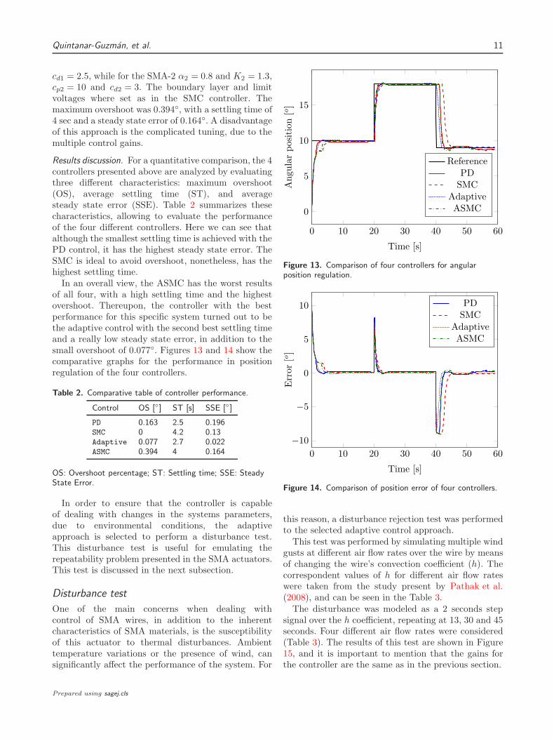
Results discussion. For a quantitative comparison, the 4controllers presented above are analyzed by evaluatingthree different characteristics: maximum overshoot(OS), average settling time (ST), and averagesteady state error (SSE). Table 2 summarizes thesecharacteristics, allowing to evaluate the performanceof the four different controllers. Here we can see thatalthough the smallest settling time is achieved with thePD control, it has the highest steady state error. TheSMC is ideal to avoid overshoot, nonetheless, has thehighest settling time.In an overall view, the ASMC has the worst results

of all four, with a high settling time and the highestovershoot. Thereupon, the controller with the bestperformance for this specific system turned out to bethe adaptive control with the second best settling timeand a really low steady state error, in addition to thesmall overshoot of 0.077. Figures 13 and 14 show thecomparative graphs for the performance in positionregulation of the four controllers.

Table 2. Comparative table of controller performance.

Control OS [] ST [s] SSE []

PD 0.163 2.5 0.196SMC 0 4.2 0.13Adaptive 0.077 2.7 0.022ASMC 0.394 4 0.164

OS: Overshoot percentage; ST: Settling time; SSE: SteadyState Error.

In order to ensure that the controller is capableof dealing with changes in the systems parameters,due to environmental conditions, the adaptiveapproach is selected to perform a disturbance test.This disturbance test is useful for emulating therepeatability problem presented in the SMA actuators.This test is discussed in the next subsection.

Disturbance test

One of the main concerns when dealing withcontrol of SMA wires, in addition to the inherentcharacteristics of SMA materials, is the susceptibilityof this actuator to thermal disturbances. Ambienttemperature variations or the presence of wind, cansignificantly affect the performance of the system. For

0 10 20 30 40 50 60

0

5

10

15

Time [s]

Angularposition[o]

ReferencePDSMC

AdaptiveASMC

Figure 13. Comparison of four controllers for angularposition regulation.

0 10 20 30 40 50 60

−10

−5

0

5

10

Time [s]

Error[o]

PDSMC

AdaptiveASMC

Figure 14. Comparison of position error of four controllers.

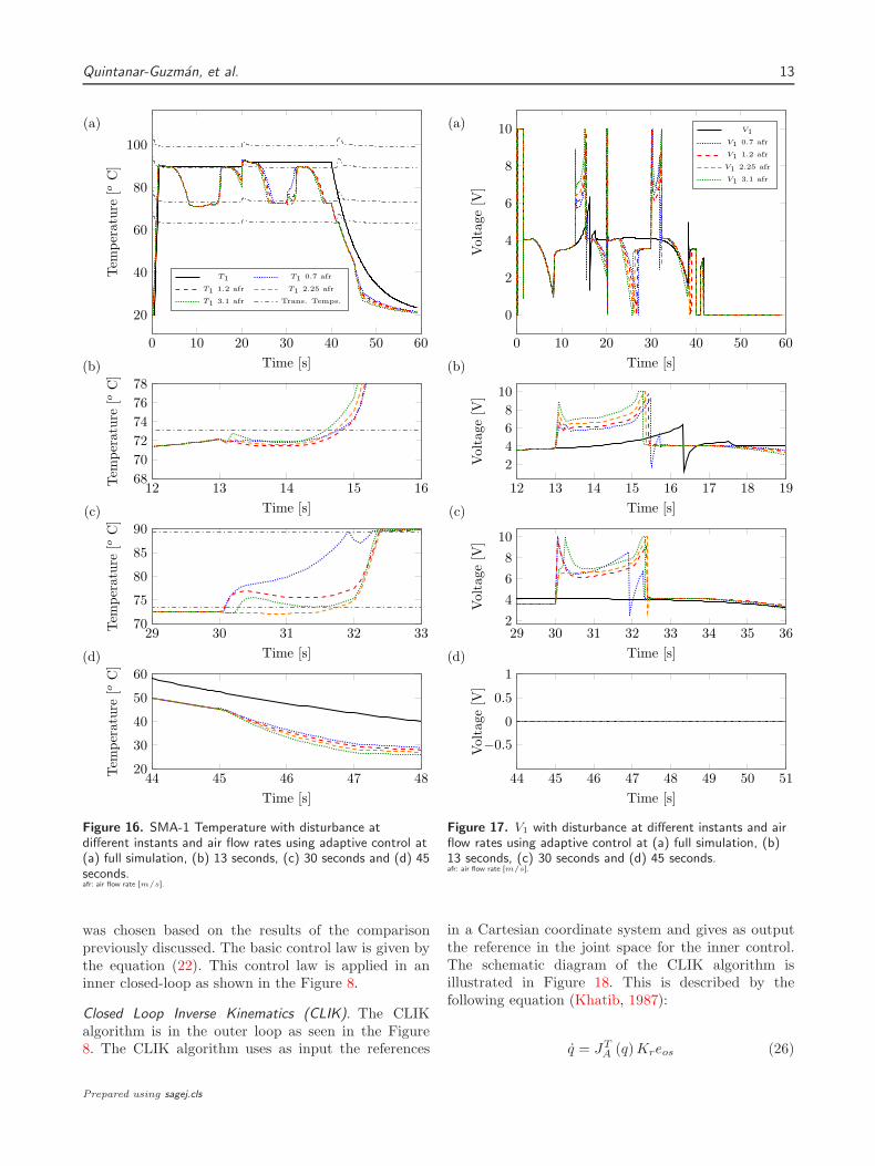
this reason, a disturbance rejection test was performedto the selected adaptive control approach.This test was performed by simulating multiple wind

gusts at different air flow rates over the wire by meansof changing the wire’s convection coefficient (h). Thecorrespondent values of h for different air flow rateswere taken from the study present by Pathak et al.(2008), and can be seen in the Table 3.The disturbance was modeled as a 2 seconds step

signal over the h coefficient, repeating at 13, 30 and 45seconds. Four different air flow rates were considered(Table 3). The results of this test are shown in Figure15, and it is important to mention that the gains forthe controller are the same as in the previous section.



Table 3. Effect of air flow rate at 22 oC on the convectioncoefficient for a 0.25 mm diameter SMA wire.

Flow rate [m/s] h [W/m2K]

0 1200.7 2301.2 3802.25 4303.1 490

Note: Data from study presented in Pathak et al. (2008).

In Figure 15(a) we can observe the completesimulation with disturbances at 13, 30 and 45 secondsat different air flow rates. In addition, Figure 15 (b) to(d) present a closer look at the time of the disturbance,where the effect of the thermal disturbance is evident,we can observe a maximum deviation of 0.2o fromreference in the worst case scenario (air flow rate of 3.1m/s). The effect of the disturbance is easily observedin Figure 16, where changes on SMA-1 temperature(T1) due to presence of disturbances, are shown.Figure 16(a) shows the complete simulation, where thethermal disturbance is really noticeable compared tothe thermal dynamic of the non perturbed system. Thiscan also be observed in Figure 17 which shows thevoltage of the SMA-1 (V1). In Figures 17(b) and (c)the controller reacts to the disturbance by increasingthe voltage to compensate the fast cooling induced bythe forced air convection. For the disturbance at 45seconds (Figure 17(d)) there is no response from thecontroller thus it is already at the lowest voltage (0V).

From this test we can conclude that the selectedadaptive control is capable of dealing with one ofthe most common disturbances affecting SMA wires(thermal disturbance). The adaptive approach is thenused for the design of the operational space control,discussed in the next section.

Operational space control: Position regulation

The operational space is a framework used toanalyze the system from the end-effector’s dynamicbehavior (Khatib, 1987). Based on this approachthe development of an operational space positioncontrol will be discussed in this section. The controllaw presented here is decomposed into two separatecontrollers. First, the inner control law that worksin the joint space, which regulates the output angleof the actuator θ1. Second part is the Closed LoopInverse Kinematics (CLIK) algorithm in the outerloop which generates the required joint space referencenecessary to control the position of the end-effector

0 10 20 30 40 50 60

0

5

10

15

20

Time [s]

AngularPosition[o]

θ1 θ1 0.7 afr

θ1 1.2 afr θ1 2.25 afr

θ1 3.1 afr

(a)

12 13 14 15 16 17 18 19

9.6

9.8

10

10.2

10.4

Time [s]

AngularPosition[o](b)

29 30 31 32 33 34 35 36

17.6

17.8

18

18.2

Time [s]

AngularPosition[o](c)

44 45 46 47 48 49 50 51

8.6

8.8

9

9.2

9.4

Time [s]

AngularPosition[o](d)

Figure 15. Angular position with disturbance at differentinstants and air flow rates using adaptive control at (a) fullsimulation, (b) 13 seconds, (c) 30 seconds and (d) 45seconds.afr: air flow rate [m/s]; Trans. Temps.: Transformations temperatures.

in the Cartesian space. The control law and theCLIK algorithm are explained in further detail in thefollowing subsections.

Inner Control Law. The inner control law regulates therotational movement of the end effector. The controlledvariable is the angular position of coupler-1 (θ1) (seeFigure 1). For the inner control, an adaptive controller



0 10 20 30 40 50 60

20

40

60

80

100

Time [s]

Tem

perature

[oC]

T1 T1 0.7 afr

T1 1.2 afr T1 2.25 afr

T1 3.1 afr Trans. Temps.

(a)

12 13 14 15 1668

70

72

74

76

78

Time [s]

Tem

perature

[oC]

(b)

29 30 31 32 3370

75

80

85

90

Time [s]

Tem

perature

[oC]

(c)

44 45 46 47 4820

30

40

50

60

Time [s]

Tem

perature

[oC]

(d)

Figure 16. SMA-1 Temperature with disturbance atdifferent instants and air flow rates using adaptive control at(a) full simulation, (b) 13 seconds, (c) 30 seconds and (d) 45seconds.afr: air flow rate [m/s].

was chosen based on the results of the comparisonpreviously discussed. The basic control law is given bythe equation (22). This control law is applied in aninner closed-loop as shown in the Figure 8.

Closed Loop Inverse Kinematics (CLIK). The CLIKalgorithm is in the outer loop as seen in the Figure8. The CLIK algorithm uses as input the references

0 10 20 30 40 50 60

0

2

4

6

8

10

Time [s]

Voltage[V

]

V1

V1 0.7 afr

V1 1.2 afr

V1 2.25 afr

V1 3.1 afr

(a)

12 13 14 15 16 17 18 19

2

4

6

8

10

Time [s]

Voltage[V

]

(b)

29 30 31 32 33 34 35 362

4

6

8

10

Time [s]

Voltage[V

]

(c)

44 45 46 47 48 49 50 51

−0.5

0

0.5

1

Time [s]

Voltage[V

]

(d)

Figure 17. V1 with disturbance at different instants and airflow rates using adaptive control at (a) full simulation, (b)13 seconds, (c) 30 seconds and (d) 45 seconds.afr: air flow rate [m/s].

in a Cartesian coordinate system and gives as outputthe reference in the joint space for the inner control.The schematic diagram of the CLIK algorithm isillustrated in Figure 18. This is described by thefollowing equation (Khatib, 1987):

q = JTA (q)Kreos (26)



Kr JTA (q)

∫

Kop (•)

Closed Loop Inverse Kinematics

xd qq

xe

Figure 18. Closed Loop Inverse Kinematics block diagram.

where q is the derivative of the state vector with respectto the time, JA is the analytical Jacobian of the roboticarm, Kr ∈ R

n is a symmetric gain matrix, n is thenumber of states in the dynamic model and eos is theoperational space error defined as:

eos = xd − xe (27)

herein, xd is the set of Cartesian coordinates forthe end effector’s desired position and xe is the endeffector’s position vector. This control represents asimple proportional control, which takes into accountthe direct and inverse dynamics of the one DOF robotarm. Equation (28) shows the analytical Jacobian ofthe robotic system and the equation (29) describes thedirect kinematics as follows:

JA (q) =∂Kop (·)

∂q=

[

−a1 sin (q1)−a1 cos (q1)

]

(28)

Kop (·) =

[

a1 cos (q1)a1 sin (q1)− h

]

(29)

where a1 is the length of the second link (150 mm), his the length of the first link (100 mm) plus the baseheight (50 mm) and we define q = θ1.The open and closed loop performance of the

SMA actuated robotic arm was evaluated throughsimulations using Simulink/MATLAB. The open-looptest was performed by applying the maximum safevoltage (V1H) to the SMA-1 while no voltage wasapplied to SMA-2 and then vice versa. The resultsof this simulation are shown in the Figure 19. Thisfigure shows the major hysteresis loop (Temperature -Strain).The plot of the hysteresis curve shows a double

hysteresis loop, however we can assume a big differencein size between the two loops. This phenomenon isdue to the use of 2 SMA wires configuration, calledas antagonistic configuration. Nonetheless, this systemis not an antagonistic application in the common sense,since the second wire does not really actuate the

20 40 60 80 100 120 140

0

1

2

3

4·10−2

Strain

Tem

perature[oC]

Figure 19. Open-loop system hysteresis curve Temperature -Strain.

end-effector, but just permits to adjust the overallstiffness of the joint.In order to carry out a closed-loop analysis, a

position regulation was performed. The step responsetest was used with a sequence of 3 steps apart by 20seconds with an amplitude computed by equation (30).This is shown in Figure 20 (solid line).

xd =

[

a1 cos (N (i)π/180)a1 sin (N (i)π/180)− h

]

(30)

where N = [10, 18, 9]. The origin of the system is set atthe center of the upper face of the robotic arm’s base.The Closed Loop Inverse Kinematics gain (Kr) was

set to 300, in order to achieve a fast response throughthis controller. The gains for the adaptive control wereset as follows: α1 = 0.9, α2 = 0.8, K1 = 19, K2 = 13,and voltage limits V1H = 10 V, V2H = 10 V. Theresults of this simulation are shown in the Figures 20to 21.In the Figure 20 it can be seen that the overshoot is

almost nonexistent with a maximum positive overshootof 0.3 % and 0.156 % for axisX and Z respectively, and0.03 % and 2.39 % for the negative one in each axis.This is attributed to the derivative effect in the filterederror. In addition, the maximum steady state error inthe X-axis was 0.002% and 0.006% for the Z-axis.Figure 21 shows the error norm of the system, withmaximum value of 0.0284 during the biggest down step.Furthermore, the system presents an average settlingtime of 4.2 seconds.The SMA wires’ temperatures and transformation

temperatures are shown in the Figure 22, where



0 10 20 30 40 50 60

−0.14

−0.12

−0.1

Time [s]

Position[m

]

ydy

(b)

0 10 20 30 40 50 60

0.14

0.14

0.15

0.15

Time [s]

Position[m

]

xd

x

(a)

Figure 20. Operational space control for position regulationstep response (a) X axis (b) Z axis.

0 10 20 30 40 50 60

0

1

2

3·10−2

Time [s]

Error

Figure 21. Step response error norm.

we can observe the influence of SMA-2 over thecooling dynamic of the system from t=40 seconds.When SMA-2 reaches the austenite transformationtemperature it causes an increment on the stress,which at the same time leads to a rise inthe transformation temperatures of SMA-1. Thiseffect simultaneously leads to an accelerated inverse

0 10 20 30 40 50 60

50

100

Time [s]Tem

perature

[oC]

T2 As

Af Ms

Mf(b)

0 10 20 30 40 50 60

50

100

Time [s]

Tem

perature

[oC]

T1 As

Af Ms

Mf

(a)

Figure 22. Temperature vs Transformation temperatures,(a) SMA-1 (b) SMA-2

transformation austenite to martensite, allowing thesystem to reach the lower reference faster.Figure 23 illustrates the control signals applied to the

system during the closed-loop test. The control signalis given in Volts and it is limited to avoid thermaldamage to the SMA wires; as an excess voltage candestroy its memory effect. The gains of the systemare tuned heuristically to achieve a faster and moreaccurate response. Table 4 shows the gains used for theadaptive controllers to regulate each SMA wire. Thegains of the SMA-2 are noticeably smaller than thoseof the SMA-1, since the SMA-2 adjusts the stiffness ofthe joint. This means that the SMA-2 does not actuatedirectly the end-effector, thus its rate of response is notas critical as SMA-1.

Table 4. Adaptive Control gains.

Wire K Γ α

SMA-1 19 5 0.9SMA-2 13 2.5 0.85

Conclusions

In this paper we have presented a SMA wire actuatedlightweight robotic arm, which is intended to be analternative to flying manipulators designs. This arm



0 10 20 30 40 50 60

0

2

4

6

8

10

Time [s]

Voltage[V

]

V1V2

Figure 23. Voltage input.

was actuated by a couple of antagonistic SMA wires.It has a total weight of 48 g and a range of movementup to 85 degrees on the X − Z plane.

A comparison between one biased wire vs anantagonistic system (2 SMA wires) was carried outin open and closed-loop. During this analysis, itbecame clear that the use of an antagonistic systemaccelerates the response of the system and increases theaccuracy. Following this analysis, a comparison among4 different controllers for the antagonistic system wasdeveloped. Different control approaches such as PD,SMC, Adaptive Control and ASMC were tested. Asa result of the comparative analysis, it was concludedthat the best performance was achieved by the adaptivecontrol law. Finally an operational space control wasdeveloped based on the closed loop inverse dynamicsof the arm presented.

Future work will be the construction and expe-rimental test of the presented design. In addition,the proposed SMA wires based robotic arm will beassembled as flying manipulator and attached to asmall quadcopter.

Declaration of conflicting interests

The author(s) declared no potential conflicts of interest

with respect to the research, authorship and/or publication

of this article

Funding

This research received no specific grant from any funding

agency in the public, commercial, or not-for-profit sectors.

References

Andani MT, Anderson W and Elahinia M (2015) Design,

modeling and experimental evaluation of a minimally

invasive cage for spinal fusion surgery utilizing

superelastic nitinol hinges. Journal of intelligent

material systems and structures 26(6): 631–638.

Barbarino S, Ameduri S, Lecce L and Concilio A (2009)

Wing shape control through an sma-based device.

Journal of intelligent material systems and structures

20(3): 283–296.

Bellicoso CD, Buonocore LR, Lippiello V and Siciliano B

(2015) Design, modeling and control of a 5-dof light-

weight robot arm for aerial manipulation. 2015 23rd

Mediterranean Conference on Control and Automation,

MED 2015 - Conference Proceedings : 853–858.

Colorado J, Barrientos A and Rossi C (2011) Musculos

inteligentes en robots biologicamente inspirados:

Modelado, control y actuacion. Revista Iberoamericana

de Automatica e Informatica Industrial RIAI 8(4): 385

– 396.

DYNALLOY Inc (2014a) Flexinol actuator wire

technical and design data. Available at:

http://www.dynalloy.com/tech_data_wire.php .

(accessed 26 April 2016).

DYNALLOY Inc (2014b) Technical char-

acteristics of flexinol. Available at:

http://www.dynalloy.com/pdfs/TCF1140.pdf.

(accessed 26 April 2016).

Elahinia MH and Ashrafiuon H (2002) Nonlinear control of

a shape memory alloy actuated manipulator. Journal

of Vibration and Acoustics 124(4): 566–575.

Gao F, Wang Z, Wang Y, Wang Y and Li J (2014) A

prototype of a biomimetic mantle jet propeller inspired

by cuttlefish actuated by sma wires and a theoretical

model for its jet thrust. Journal of Bionic Engineering

11(3): 412–422.

Guo Z, Pan Y, Wee LB and Yu H (2015) Design and control

of a novel compliant differential shape memory alloy

actuator. Sensors and Actuators A: Physical 225: 71–

80.

Hassani V, Tjahjowidodo T and Do TN (2014) A survey

on hysteresis modeling, identification and control.

Mechanical Systems and Signal Processing 49(12): 209

– 233.

Hulea M and Caruntu CF (2014) Spiking neural network for

controlling the artificial muscles of a humanoid robotic

arm. In: 2014 18th International Conference on System

Theory, Control and Computing (ICSTCC). IEEE, pp.

163–168.

Jafari J, Zebarjad S and Sajjadi S (2008) Effect of pre-

strain on microstructure of niti orthodontic archwires.

Materials Science and Engineering A 473(12): 42–48.


http://www.dynalloy.com/tech_data_wire.php

http://www.dynalloy.com/pdfs/TCF1140.pdf


Kannan S (2011) Modelisation et Commande dActionneurs

a Alliage a Memoire de Forme. PhD Thesis, l’Ecole

Nationale Superieure d’Arts et Metiers.

Kannan S, Bezzaoucha S, Quintanar-Guzman S, Olivares-

Mendez MA and Voos H (2016a) Adaptive control of

robotic arm with hysteretic joint. In: Proceedings of the

4th International Conference on Control, Mechatronics

and Automation, ICCMA ’16. Barcelona: ACM, pp. 46–

50.

Kannan S, Giraud-Audine C and Patoor E (2010) Laguerre

model based adaptive control of antagonistic shape

memory alloy (sma) actuator. In: Proc. SPIE 7643,

Active and Passive Smart Structures and Integrated

Systems 2010, volume 7643. pp. 764307–764307–12.

Kannan S, Giraud-Audine C and Patoor E (2013)

Application of laguerre based adaptive predictive

control to shape memory alloy (sma) actuator. ISA

Transactions 52(4): 469 – 479.

Kannan S, Quintanar-Guzman S, Bezzaoucha S, Olivares-

Mendez MA and Voos H (2016b) Adaptive control

of hysteretic robotic arm in operational space. In:

Proceedings of the 5th International Conference on

Mechatronics and Control Engineering, ICMCE ’16.

Venice: ACM, pp. 92–96.

Kennedy DK, Straub FK, Schetky LM, Chaudhry Z and

Roznoy R (2004) Development of an sma actuator for

in-flight rotor blade tracking. Journal of intelligent

material systems and structures 15(4): 235–248.

Khatib O (1987) A unified approach for motion and

force control of robot manipulators: The operational

space formulation. IEEE Journal on Robotics and

Automation 3(1): 43–53.

Khodayari A, Talari M and Kheirikhah MM (2011) Fuzzy

pid controller design for artificial finger based sma

actuators. In: 2011 IEEE International Conference on

Fuzzy Systems (FUZZ-IEEE 2011). pp. 727–732.

Ko J, Jun MB, Gilardi G, Haslam E and Park EJ (2011)

Fuzzy pwm-pid control of cocontracting antagonistic

shape memory alloy muscle pairs in an artificial finger.

Mechatronics 21(7): 1190–1202.

Landau ID, Lozano R, M’Saad M and Karimi A (2011)

Adaptive control: algorithms, analysis and applications.

Springer Science & Business Media.

Liang C and Rogers CA (1990) One-dimensional

thermomechanical constitutive relations for shape

memory materials. Journal of intelligent material

systems and structures 1(2): 207–234.

Liu J and Wang X (2011) Advanced Sliding Mode

Control for Mechanical Systems: Design, Analysis

and MATLAB Simulation. Springer-Verlag Berlin

Heidelberg.

Mai H, Song G and Liao X (2013) Adaptive online inverse

control of a shape memory alloy wire actuator using

a dynamic neural network. Smart Materials and

Structures 22(1): 015001.

Mataee MG, Andani MT and Elahinia M (2015) Adaptive

anklefoot orthoses based on superelasticity of shape

memory alloys. Journal of intelligent material systems

and structures 26(6): 639–651.

Moghaddam NS, Skoracki R, Miller M, Elahinia M

and Dean D (2016) Three dimensional printing of

stiffness-tuned, nitinol skeletal fixation hardware with

an example of mandibular segmental defect repair.

Procedia CIRP 49: 45–50.

Nematzadeh F and Sadrnezhaad S (2012) Effects of

material properties on mechanical performance of

nitinol stent designed for femoral artery: Finite element

analysis. Scientia Iranica 19(6): 1564 – 1571.

Nespoli A, Dallolio V, Villa E and Passaretti F (2015) A

new design of a nitinol ring-like wire for suturing in

deep surgical field. Materials Science and Engineering

C 56: 30–36.

Pan Y, Guo Z, Li X and Yu H (2017) Output-feedback

adaptive neural control of a compliant differential sma

actuator. IEEE Transactions on Control Systems

Technology PP(99): 1–9.

Pandis N and Bourauel CP (2010) Nickel-titanium (niti)

arch wires: the clinical significance of super elasticity.

Seminars in Orthodontics 16(4): 249–257. Latest

Controversies in Orthodontics: From in Vitro Data to

in Vivo Evidence.

Pathak A, Brei D and Luntz J (2008) Experimental

characterization of the convective heat transfer from

shape memory alloy (sma) wire to various ambient

environments. In: Student’s papers. Ascona, Switzer-

land: Pathak,A.; Mechanical Engineering, University of

Michigan, 2250 GG Brown, Ann Arbor, MI 48109-2126,

USA, [email protected], p. 12 pp.

Queiroz MS, Dawson DM, Nagarkatti SP and Zhang F

(2000) Lyapunov-Based Control of Mechanical Systems.

Springer.

Quintanar-Guzman S, Kannan S, Olivares-Mendez MA

and Voos H (2016) Operational space control of a

lightweight robotic arm actuated by shape memory

alloy (sma) wires. In: ASME 2016 Conference on

Smart Materials, Adaptive Structures and Intelligent

Systems, volume Volume 2: Modeling, Simulation and

Control; Bio-Inspired Smart Materials and Systems;

Energy Harvesting. Stowe, Vermont: American Society

of Mechanical Engineers.

Quintanar-Guzman S, Reyes-Reyes J and Arellano-Sanchez

Mdc (2014) Modelado y control de un sistema

electrotermico-mecanico movil basado en alambres



musculares. In: XVI Congreso Latinoamericano

de Control Automatico, CLCA 2014. Asociacion de

Mexico de Control Automatico, pp. 834–839.

Rao A, Srinivasa AR and Reddy JN (2015) Design of

Shape Memory Alloy (SMA) Actuators. SpringerBriefs

in Computational Mechanics. Springer International

Publishing.

Rodrigue H, Cho S, Han MW, Bhandari B, Shim JE

and Ahn SH (2016) Effect of twist morphing wing

segment on aerodynamic performance of uav. Journal

of Mechanical Science and Technology 30(1): 229–236.

Shin BH, Lee KM and Lee SY (2015) A miniaturized

tadpole robot using an electromagnetic oscillatory

actuator. Journal of Bionic Engineering 12(1): 29–36.

Son HM, Kim MY and Lee YJ (2009) Tunable-focus liquid

lens system controlled by antagonistic winding-type

sma actuator. Optics Express 17(16): 14339–14350.

Sreekumar M, Nagarajan T and Singaperumal M (2009)

Application of trained niti sma actuators in a spatial

compliant mechanism: Experimental investigations.

Materials & Design 30(8): 3020–3029.

Tai NT and Ahn KK (2012) Output feedback direct

adaptive controller for a sma actuator with a kalman

filter. IEEE Transactions on Control Systems

Technology 20(4): 1081–1091.

Tao G (2014) Multivariable adaptive control: A survey.

Automatica 50(11): 2737 – 2764.

Williams EA, Shaw G and Elahinia M (2010) Control of

an automotive shape memory alloy mirror actuator.

Mechatronics 20(5): 527–534.

Young KD, Utkin VI and Ozguner U (1999) A control

engineer’s guide to sliding mode control. IEEE

Transactions on Control Systems Technology 7(3): 328–

342.

Zheng T, Yang Y, Branson DT, Kang R, Guglielmino

E, Cianchetti M, Caldwell DG and Yang G (2014)

Control design of shape memory alloy based multi-

arm continuum robot inspired by octopus. In: 2014

IEEE 9th Conference on Industrial Electronics and

Applications (ICIEA). pp. 1108–1113.


operational space control of a c the author(s) 2017...

Documents