operations research expositions in mathcad -
TRANSCRIPT

f f
Duško Letić
Branko Davidović
Zoran Čekerevac
Zdenek Dvorak
Ivana Berković
Ljubica Kazi
Eleonora Desnica....

Contents _________________________________________________________________________________________________________
ii
Duško Letić
Branko Davidović
Zoran Čekerevac
Zdenek Dvorak
Ivana Berković
Ljubica Kazi
Eleonora Desnica
OPERATIONS RESEARCH
Expositions in Mathcad
Optimizing methods
Exame tasks
Essays
Programme solutions
CITY XXXX, 2008.
OPERATIONS RESEARCH – Expositions in Mathcad

Contents _________________________________________________________________________________________________________
i
Duško Letić, PhD
Branko Davidović, PhD
Zoran Čekerevac, PhD
Zdenek Dvorak, PhD
Ivana Berković, PhD
Ljubica Kazi, MSc
Eleonora Desnica, MSc
Reviewers: Professor Mirko Vujošević, PhD Faculty of Organizational Sciences,
Belgrade, Serbia
PhD Dragan Radojević, “Mihailo Pupin“, Institute, Belgrade, Serbia
Docent Detelin Vasilev, PhD, Higher School of Transport “Todor
Kableshkov”, Sofia, Bulgaria
Publisher:
For publisher:
Lecturer: Mr Srđan Šerer, senior lecturer.
Logo:
Contents _________________________________________________________________________________________________________
ii
Preface
The book OPERATIONS RESEARCH – Expositions in Mathcad is concise
matter made during several years of teaching at the Tecnical Faculty “Mihailo Pupin“ in
Zrenjanin. Subject matter of this book can be equaly interesting to students of many
profiles of this faculty: informatics teachers, informatics engineers, technics and
informatics teachers and to graduated engineers for management of technical systems and
to the others. The book contains algorithms in operations research field that are mostly
mathematically oriented. Its chapters treat:
Linear programming
Transpotation problem
Assignment problem of workplaces
Nonlinear programming
Dinamic programming
Multicriteria optimization
Heuristic research
Markov chains
Mass queueing
Simulation modelling (Monte-Carlo)
Game theory
Inventory control
Network planning
Testing statistical hypotheses.
After introductory informing about the history of the subject matter field, follow
the problems exposed in the chapters of the cited sequence. Each chapter contains
mathematical proceedings without detailed proofs, with accent on pragmatism and
applicability of methods and proceedings of operations research. An accompanying CD
completes the contents of the book and offers students sufficient and necessary matter
through representative files, sorted according to chapters (folders).
The authors express their acknowledgement to PhD Milan Bojanović, director of
the company CPS-CAD Professional Sys. from Belgrade and Mr Srđan Šerer, senior
lecturer of English language, for useful suggestions at final editing of this textbook.
We especially express our thanks to the reviewers of this textbook, PhD Mirko Vujošević
from the Faculty of Organizational Sciences from Belgrade, PhD Dragan Radojević from
the Institute “Mihailo Pupin” in Belgrade and doc. Detelin Vasilev, PhD, from Higher
school of transport “Todor Kableškov” in Sofia.
January, 2008
Authors

Contents _________________________________________________________________________________________________________
i
Contents [file.mcd]
OPERATIONS RESEARCH DEVELOPMENT ................................................................. 1
1. LINEAR PROGRAMMING................................. .................................................................. 2
1.1 Optimization of production program [LP1.mcd] ........................................................... 2
1.2 Optimization of vitamin [LP2.mcd] .............................................................................. 4
1.3 Optimization of production program assortment/quantity [LP3.mcd] ........................... 5
1.4 Linear programing model with two variables [LP4.mcd] .............................................. 7
1.5 Optimization of rocket number [LP5.mcd] ................................................................... 9
1.6 Raw materials quantity optimization of chemical products [LP6.mcd] ...................... 11
1.7 Dual model of linear programming [LP7.mcd] ............................................................ 13
2. TRANSPORTATION PROBLEM ................................. ..................................................... 19
2.1 Transportation problem with minimal expenses [TP1.mcd] ........................................ 19
2.2 Transport task with minimal expenses [TP2.mcd] ....................................................... 21
2.3 Transport problem of profit maximum [TP3.mcd] ....................................................... 23
2.4 Transport problem of profit maximum [TP4.mcd] ....................................................... 25
2.5 Transport problem of minimum expenses [TP5.mcd] .................................................. 28
2.6 Transport problem of minimum of expenses [TP6.mcd] ............................................. 30
2.7 Transport problem of minimum of expenses [TP7.mcd] ............................................. 32
3. ASSIGNMENT PROBLEM ................................. ................................................................ 35
3.1 Employees assignment [AP1a.mcd] ............................................................................. 35
3.2 Arrangement of jobs [AP2a.mcd] ................................................................................. 37
3.3 Job disposition [AP2a_2.mcd] ...................................................................................... 39
3.4 The open problem of jobs disposition [AP3.mcd] ........................................................ 42
3.5 Disposition of students [AP4.mcd] ............................................................................... 44
4. NONLINEAR PROGRAMMING ................................. ...................................................... 48
4.1 A model of nonlinear programming [NP1.mcd] ........................................................... 48
4.2 Profit maximization through nonlinear programming method [NP2.mcd] .................. 52
4.3 Conditions of production optimality (optimum) [NP3.mcd] ....................................... 53
4.4 Utility function-optimal volume of purchase of goods [NP4.mcd] ............................. 53
4.5 Optimization of enzyme product [NP5.mcd] .............................................................. 55
5. DYNAMIC PROGRAMMING ...................................................... ...................................... 57
5.1 One-dimensional process of optimal resources distribution [DP1.mcd] ...................... 57
6. MULTICRITERIA OPTIMIZATION ...................................... ......................................... 61
6.1 The method of simple additive weights [MO1.mcd] .................................................... 61
7. HEURISTIC RESEARCH ................................. .................................................................. 62
7.1 Optimal pipeline diameter [HR1.mcd] ......................................................................... 62
8. MARKOV MODELS ................................. ........................................................................... 65
8.1 The model for forecast consumers’ orientation [MM1.mcd] ....................................... 65
8.2 Negotiability of assets (Credits, demands) [MM2.mcd] .............................................. 67
9. MASS QUEUEING ................................. .............................................................................. 69
9.1 The system of queueing M/G/1/ infinite [MQ1.mcd] .................................................... 69
9.2 Sixchannel model of mass queueing [MQ2.mcd]......................................................... 70
10. SIMULATION MODELING ................................. ............................................................. 71
10.1 Random number generation [SM16.mcd] .................................................................. 71
10.2 Simulating time reliability of technical system elements [SM16a.mcd] .................... 74
11. MATRIX GAMES ................................. .............................................................................. 77

Contents _________________________________________________________________________________________________________
ii
11.1 Nonsingular matrix games [MG1.mcd] ...................................................................... 77
12. INVENTORY CONTROL ................................. ................................................................. 78
12.1 The calculation of optimal quantities of inventory with constant
procurement [IC1.mcd] .............................................................................................. 78
12.2 Calculation of optimal inventory quantities with intervened order [IC2.mcd] ........... 81
13. NETWORK PLANNING ................................. ................................................................... 83
13.1 Application of network technique PERT [PN1.mcd] ................................................. 83
14. TESTING STATISTICAL HYPOTHESES ................................. ..................................... 84
14.1 Test χ2 for verification the hypothesis about composition of empirical with
theoretical exponential distribution [ST1.mcd].......................................................... 83
14.2 Testirng hypothesis about samples homogenity in view of their
variances [ST2.mcd] .................................................................................................. 90
Reference .. ................................................................................................................................... 92
Basic Structure of OR Tutorial
MASS QUEUEING
MMMM
MQMQ
SMSM
MGMG
ICIC
NINI
STST
MARKOV MODELS
NETWORK PLANNING
INVENTORY CONTROL
SIMULATION MODELING
LINEAR PROGRAMMINGLP
LP
TPTP
APAP
NPNP
DPDP
TRANSPORTATION PROBLEM
ASSIGNMENT PROBLEM
NONLINEAR PROGRAMMING MATRIX GAMES
TESTING STATISTICAL
HYPOTHESES
MOMO
HRHR
DYNAMIC PROGRAMMING
MULTICRITERIA OPTIMIZATION
HEURISTIC RESEARCH
Note All textual and/or picture information published in this book and taken over from the site
PTC, are taken on by consent of CPS-CAD Professional Sys. Company, Belgrade, that is official
distributor of the software package Mathcad for the Republic of Serbia. To the editor printing of
the book is approved.


Operations Research __________________________________________________________________________________________________________
1
OPERATIONS RESEARCH DEVELOPMENT
n computer mathematics, for models of often very complex structures, very quickly are
being developed numerical methods of optimization. Their problems are studying
exxtreme values of criteria functions with argument optimal values. We need to stress
especially tasks of mathematical programming. Knowing their essentials, we can solve
many tasks in production and business. Operations research and management science include also
optimization tasks, as well appropriate methods elaborated for their solving. Stability of
computing methods and algorithms comprises one of main trends in researching the application
and classification of various mistakes with implementing these methods. In the beginning of the
20th century, in 1916, begins development of management science, founded by Frederick Taylor
[2]. With this have been sloved several substantial matters, and they, predominantly, refer to
resources management. In those years Harris has set fundamental mathematical model of optimal
inventory level. The emergence of queueing theory referred to Danish mathematician A.K. Erlang
(1909). Their contributions to the theory of optimal inventory have given, among others: Kendal,
Lee, Hinchin and Polachek. Game theory is mathematical theory about decision making in
competitor situations of opposite interests. The first to begin its developing, was Emile Borel in
1921, and fundamental contribution was given in 1928 by Von Neumann (1903-1957). Its first
examples of modelling linear programming and transport problem were exposed in Kantorovich’s
papers in 1939, and in Neumann’s work in 1936. Sudden development of this theory and praxis
followed after the second world war. A transportation problem pioneer is also American
mathematician Hitchcock from 1941. He was one of the first to formilate and solve one type of
transportation assignments. There are also Vogel’s papers dedicated to the approximate method
for finding the initial transport solution. The papers of Ford, Falkerson, Charnes, Cuper and
others. All these were preconditions to form a team of acientists on the eve of the second world
war in Great Britain. They were from different fields but they were included into researches of
multiple operations connected to coordination and arrangement of radar systems, military
resources transport and the like. These operations researchers have used mathematical methods,
and so they have created multidisciplinary science named Operations research. After the war its
methods were very quickly implemented solving problems in production and business, medicine,
industry and the like. Great importance had simplex, a linear programming method developed in
1947 by a famous American mathematician Danzing [9]. In the period 1951-1955 this nethod was
modificated by Charens, Lemke and Danzig himself [9]. During fifties were being strongly
sressed linear programming and statistical methods. During the same decade Neumann and
Morgenstern have set a modern game theory. Since Neumann the term “games“ has been used as
a scientific metaphor for communication among the expers for whom is substantial result of
mutual strategies interaction of two or more parties that have conflict interests. The fifties were
marked by the beginnings of non-linear programming by Kun and Tucker. This have coused
eventful development of new methods and applying of operations research. The known numerical
simulation method Monte Carlo was created in 1948, when appeared the paper of Metropolis and
Ulman about random numbers. It has been used both for solving deterministic and stohastic tasks
in many scientific spheres: reliability theory, meteorology, production, mass queueing, nuclear
physics and the like. As logical continuation of traditional Gant’s diagram aplying towards the
end of fifties of last century, there was developed the set of methods that is called network
planning technologies. These methods are established on results of algebra, graph theory,
statistics and computing sciences. The first study with essential assumptions of this method was
published by Valker and Kelly in 1958. The development of PERT method began in 1958. The
I
Expositions in Mathcad __________________________________________________________________________________________________________
2
research was led by Fazar and mathematical bases of the method were established by Clark in
1958 [15]. Dynamic programming (DP) and algorithms of optimal management were set by
American scientist Belman in 1952. He developed classical methodology for modelling and
solving of one class of specially structured optimizing tasks connected with so-called multiphasal
management processes. During 1960s great influence have had: network planning, linear
programming, graph theory in optimization and discrete stohastic simulation. 1970s are
characteristic with non-linear programming and global optimization, as well with computer
methods based on numerical mathematics. Then have been significantly developed theoretical
bases with new algorithms in uncertainty approach, when classical statistical and probability
models have not been any more exclusively used. A significant technology was developed in the
behinning of 70s. It was named PDM or “precedence diagramming method“. The algorithms of
this method are built today in nearly all program packets for network planning. So, this highly
elaborated technology is perhaps most of all others from the research field, applicable in praxis.
In 80s the attention of operations research is directed to multicriteria optimiyation and decision
making theory. Expert systems and the systems for decision making support enable introucting
personal computers with appropriate program support. More recent methods, established on the
theory of “fuzzy sets“ in the world of science were published by Zadeh in 1965. Nowdays there
are numerous methods based on fuzzy principle: “As closer we watch real problem, its solution
becomes more and more fuzzy“ (Zadeh), so that the theory of fuzzy sets has appropriately been
applied in technical systems management [3], [25]. During 90s have been done significant
penetrations in solving the problems of integer, mixed and multicriteria programming. Enrmous
computer resources become mass available and enable efficient application of operations research
method in daily real systems and processes. The development of new approaches for solving such
problems, comprises on the basis of heuristics: genetic algorithms, neuron networks and the like.
Gradually were being created the tools for solving the problems that will be applicated in new
technological circumstances, internet environment and electronic business. Besides, we can say
that an incomplete evolution in terminology has happened, so that nowdays, attention is paid to
operational management, not only to their research.
1. LINEAR PROGRAMMING
1.1 Optimization of production program [LP1.mcd]
Example The factory produces two types of products P1 and P2. The production is being run on
two machines. For the first product processing the operation times are: 4 hours/piece on the first
machine and 10 hours/piece on the second machine. For processing the second product, these
times are: 5 hours/piece on the first machine, and 6 hours/piece on the second machine. Effective
capacities of the machines can be used to the atmost 750 and 850 hours respectively. The
products appear at the market with minimal quantity of 40 pieces for P1 and 65 pieces for P2.
Determine maximal production profit and optimal product quantities by the linear programming
method, if the product unit prices are c1= 5500 mu/piece (mu=monetary unit) for P1 and c2 =
2800 mu/piece for P2.

Operations Research __________________________________________________________________________________________________________
3
Solution:
Criterion function (profit): F x( ) 5500 x0
2800 x1
In that case the vector of the products price is: C 5500 2800( )
Constraints in respect of production and market are:
production: 4 x0
5 x1
750 10 x0
6 x1
850
market: x0
40 x1
65
On account of equalization of relational operators of all four constraints, the last two non-
equations can be defined as:
A
4
10
1
0
5
6
0
1
B
750
850
40
65
One initial value (it is supposed for the last variable): x1
50
The block for solving the model of linear programming:
Given A x B x 40
The optimal quantities of products P1 and P2 of the production program:
so the optimal values are: Xr46
65
or apart: Xr0
46 Xr1
65
The maximum company profit is: D C Xr D 435000
Arithmetical an logical solution verification are: A Xr
509
850
46
65
and A Xr 0
1
1
0
0
Xr MaximizeF x( )

Expositions in Mathcad __________________________________________________________________________________________________________
4
Supplementory variables are: Xd A Xr B Xd
241
0
6
0
Note Alternative procedures for solving this problem are given at the files LP1_1.mcd.
1.2 Optimization of vitamin [LP2.mcd]
Example For the production of the vitamin tablets T1, T2 and T3 one factory that produces
pharmaceuticals uses the raw materials S1, S2, S3 and S4. The number of vitamin tablets one can
get out of one kilogram of raw material is presented in the next table [16].
T.1.1
iT
T1 8
S1
T2 4
T3 4
jS
6
S2
4
2
4
S3
2
8
4
S4
6
2
18000
Need of tablets
(pieces)
12000
8000
During planned period it is necessary to produce 18000, 12000 and 8000 vitamin tablets T1, T2
and T3. One kilogram of raw material S1, S2, S3 and S4 one can buy at the market at the price of
16, 24 15 and 20 /mu/. If raw material supplying Sj has no constraints, one must determine
optimal plan of raw materials aquisition with least total expenses.
Solution
Let x1, x2, x3 and x4 reprezents kilogram number of raw materials S1, S2, S3 and S4, then the
model of raw materials acquisition has the form:
8 x1
6 x2
4 x3
4 x4
18000
4 x1
4 x2
2 x3
6 x4
12000
4 x1
2 x2
8 x3
2 x4
8000
The matrix of coefficiants and the constraints vector on the basis of the equation system is now:
A
8
4
4
6
4
2
4
2
8
4
6
2
B
18000
12000
8000
ORIGIN 1
The criterion function is formed as: F x( ) 16 x1
24 x2
15 x3
20 x4
Operations Research __________________________________________________________________________________________________________
5
Where the price vector is: C 16 24 15 20( )
One initial value (it is supposed for the last variable): x4
0
The block for solving the model of linear programming:
Given A x B x 0
The optimal variants of cutting out bars: X MinimizeF x( )
so, the optimal values are: XT
1250 1000 0 500( )
The optimal plan presents next values of raw materials quantity /kg/:
X1
1250 X2
1000 X3
0 X4
500
The minimum aggregate expenses of raw materials acquisition for the production of the planned
number of vitamin tablets are /mu/:
T C X T 54000
The verification of solution: A X
18000
12000
8000
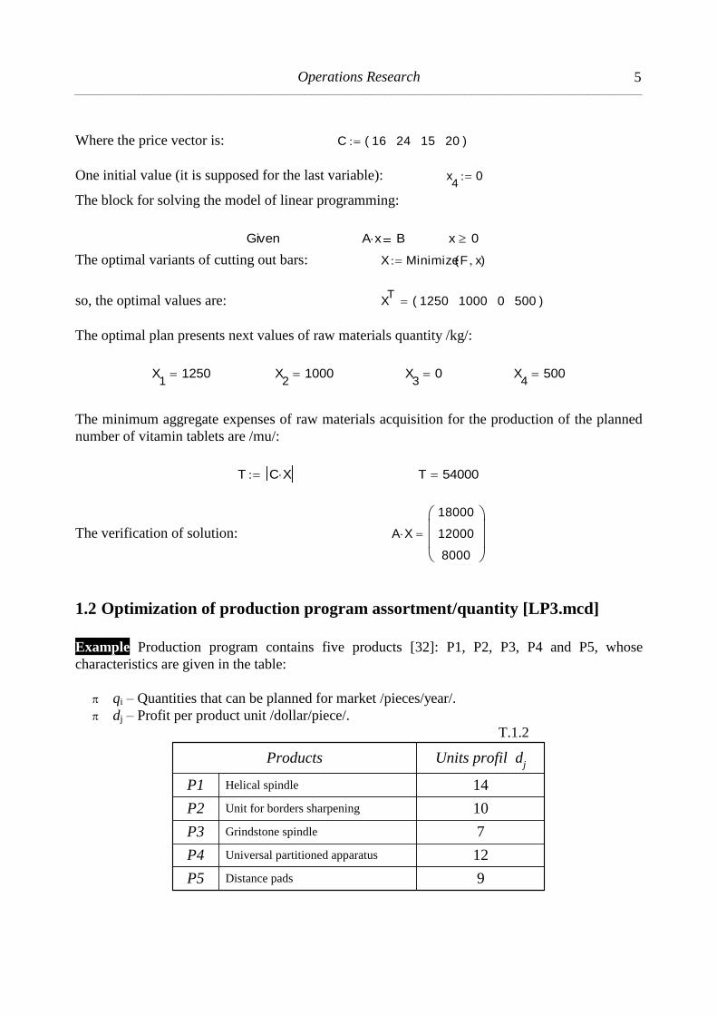
1.2 Optimization of production program assortment/quantity [LP3.mcd]
Example Production program contains five products [32]: P1, P2, P3, P4 and P5, whose
characteristics are given in the table:
qi – Quantities that can be planned for market /pieces/year/.
dj – Profit per product unit /dollar/piece/.
T.1.2
P1
Products
P2
P3
P4
P5
Helical spindle
Unit for borders sharpening
Grindstone spindle
Universal partitioned apparatus
Distance pads
Units profil dj
14
10
7
12
9

Expositions in Mathcad __________________________________________________________________________________________________________
6
In the work process analysis for the production of five planned products, besides others, have
taken part five kinds of technological systems as like:
US – universal lathes CNC, with capacity of 50000 hours/year.
OC – process centres, with capacity of 80000 hours/year.
BK – coordinative drilling machines, with capacity of 40000 hours/year.
BR – grinder for flat grinding, with capacity of 50000 hours/year.
BN – grinder for thread grinding, with capacity of 20000 hours/year.
Here, time standard for products /hours/year/ and given sorts of technological systems is
presented in the next table.
T.1.3
US
OC
BK
BR
BN
2
4
1
1
5
P1
5
25
20
4
-
P2
4
15
5
10
-
P3
25
20
2
18
-
P4
10
-
1
20
-
P5
ProductsTechnological
systems
50000
80000
40000
50000
20000
Time capacities
/hours/
Production program optimization will be realised in compliance with the above described LP
model in which criterion function is given as the need for profit maximization.
System variable: ORIGIN 1
Criterion function (profit) is: F x( ) 14 x1
10 x2
7 x3
12 x4
9 x5
The constraints defined only by thime capacities of technological systems are:
2 x1
5 x2
4 x3
25 x4
10 x5
50000
4 x1
25 x2
15 x3
20 x4
80000
x1
20 x2
5 x3
2 x4
x5
40000
x1
4 x2
10 x3
18 x4
20 x5
50000
5 x1
20000
It is necessary to formalize the previous LP model in the form of matrices and vectors as:
The vector of prices: C 14 10 7 12 9( )

Operations Research __________________________________________________________________________________________________________
7
The matrix of coefficients (operation times) A and constraints vector (time capacities) B:
A
2
4
1
1
5
5
25
20
4
0
4
15
5
10
0
25
20
2
18
0
10
0
1
20
0
B
50000
80000
40000
50000
20000
The solution follows on the basis of the defined model through the matrix A and the vectors B
and C, with the supposed initial value (as the last variable in non-equation system):
x5
0
LP block for solving: Given
A x B x 0
The optimal solution for products
quantity:
or apart:
Xr1
4000 Xr2
1547.61 Xr3
453.12 Xr4
925.64 Xr5
930.84
The maximal profit is: D C Xr D 94133.24
The verification of arithmetical and logical solution:
A Xr
50000
80000
40000
50000
20000
A Xr B
1
1
1
1
1
(True)
The additional variables are: Xd A Xr B respectively: Xd
0
0
0
0
0
Xr Maximize F x( ) Xr
4000
1547.61
453.12
925.64
930.84

Expositions in Mathcad __________________________________________________________________________________________________________
8
1.4 Linear programing model with two variables [LP4.mcd]
Example For the given criterion function and the non-equation system with two unknowns, apply
the method of optimum solving of unknown arguments and maximum of criterion funciton. On
the basis of LP model form graphical and animation presentation of the solution.
Solution
Criterion function (max): F x( ) 2 x1
2 x2
(ORIGIN 1 )
The system of linear constraints:
x1
2 x2
8 x1
x2
1 x1
2 x2
04
5x1
2 x2
3
On account of equalling relativ operators the last two non-equations can be written as:
x1
2 x2
04
5 x
1 2 x
2 3
On the basis of previous LP model follows the matrix of coefficients and the constraints vector:
A
1
1
1
4
5
2
1
2
2
B
8
1
0
3
On the basis ov previous LP model, follows the matrix of coefficients and the constraints vector.
The initial value of one unknown (the last variable): x
21
Block for solving and LP system: Given A x B x 0
Optimal solution of LP model: Xr MaximizeF x( ) so: Xr4
2
Maximal value of criterion function is: F C Xr F 12
Operations Research __________________________________________________________________________________________________________
9
The solution verification: A Xr
8
2
0
7.2
A Xr B
0
3
0
4.2
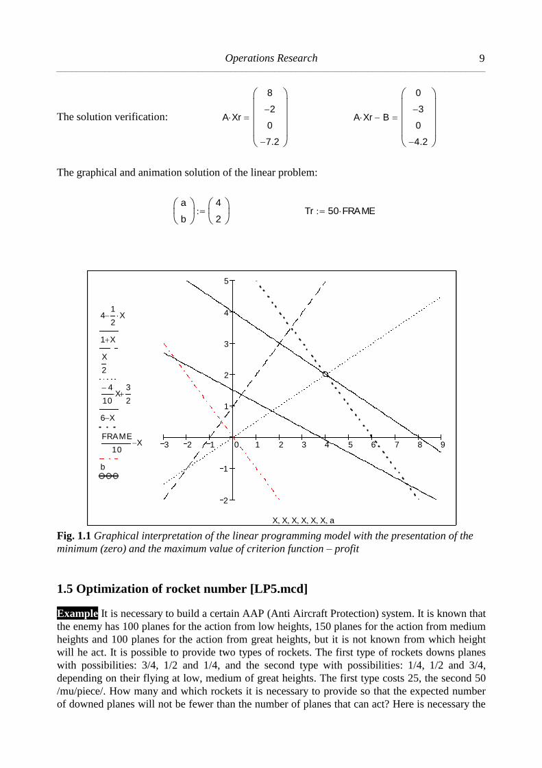
The graphical and animation solution of the linear problem:
a
b
4
2
Tr 50 FRAME
3 2 1 0 1 2 3 4 5 6 7 8 9
2
1
1
2
3
4
5
41
2X
1 X
X
2
4
10X
3
2
6 X
FRAME
10X
b
X X X X X X a
Fig. 1.1 Graphical interpretation of the linear programming model with the presentation of the
minimum (zero) and the maximum value of criterion function – profit
1.5 Optimization of rocket number [LP5.mcd]
Example It is necessary to build a certain AAP (Anti Aircraft Protection) system. It is known that
the enemy has 100 planes for the action from low heights, 150 planes for the action from medium
heights and 100 planes for the action from great heights, but it is not known from which height
will he act. It is possible to provide two types of rockets. The first type of rockets downs planes
with possibilities: 3/4, 1/2 and 1/4, and the second type with possibilities: 1/4, 1/2 and 3/4,
depending on their flying at low, medium of great heights. The first type costs 25, the second 50
/mu/piece/. How many and which rockets it is necessary to provide so that the expected number
of downed planes will not be fewer than the number of planes that can act? Here is necessary the

Expositions in Mathcad __________________________________________________________________________________________________________
10
expenses for acquisition reduce to the minimum possible measure, and to present the solution
fraphically [20].
Solution
Criterion function (expenses): ORIGIN 1 F x( ) 25 x1
50 x2
In that case the vector of cost price is: C 25 50( )
The constraints system concerning number of downed planes:
3
4x1
1
4x2
1001
2x1
1
2x2
1501
4x1
3
4x2
100
The matrix of coefficeints and constraints vector on the basis of the non-equation system is now:
A
3
4
1
2
1
4
1
4
1
2
3
4
B
100
150
100
One initial value (it is supposed for the last variable): x2
0
The block for solving linear programming model: Given
A x B x 0
The optimal rocket quantities: X MinimizeF x( ) X250
50
So, for construction an efficient AAP system, it is necessary to provide the next number of
rockets:
X1
250 X2
50
The minimum value of criterion function is: T C X T 8750
The verification of solution: A X
200
150
100
Operations Research __________________________________________________________________________________________________________
11
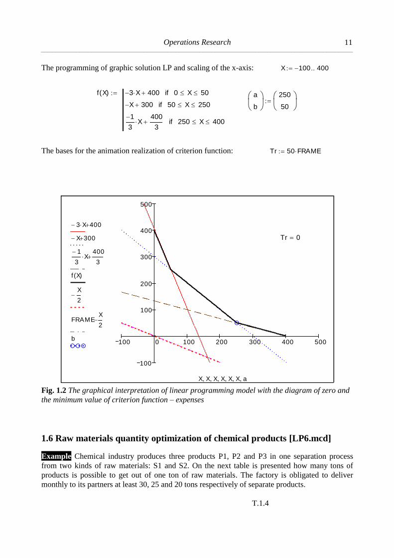
The programming of graphic solution LP and scaling of the x-axis: X 100 400
f X( ) 3 X 400 0 X 50if
X 300 50 X 250if
1
3X
400
3 250 X 400if
a
b
250
50
The bases for the animation realization of criterion function: Tr 50 FRAME
100 0 100 200 300 400 500
100
100
200
300
400
500
3 X 400
X 300
1
3X
400
3
f X( )
X
2
FRAMEX
2
b
X X X X X X a
Tr 0
Fig. 1.2 The graphical interpretation of linear programming model with the diagram of zero and
the minimum value of criterion function – expenses
1.6 Raw materials quantity optimization of chemical products [LP6.mcd]
Example Chemical industry produces three products P1, P2 and P3 in one separation process
from two kinds of raw materials: S1 and S2. On the next table is presented how many tons of
products is possible to get out of one ton of raw materials. The factory is obligated to deliver
monthly to its partners at least 30, 25 and 20 tons respectively of separate products.
T.1.4

Expositions in Mathcad __________________________________________________________________________________________________________
12
iS
S1 0,03
P1
S2 0,6
jP
0,125
P2
0,25
0,4
P3
0,05
Quantity of products
(tons)30 25 20
a) How many tons of raw materials is necessary to supply the commercial department of
chemical industry ant the price of 500 and 400 /mu/ respectively, so that the expanses are
minimal.
b) Out of which product we can deliver more to the partners than the lower limit is.
c) Present in graphical and animation way the solution for the LP model.
Solution
Constraints system with regard to non-equations: (ORIGIN 1 )
0.03 x1
0.6 x2
30 0.125 x1
0.25 x2
25 0.4 x1
0.05 x2
20
Criterion function (expenses): F x( ) 500 x1
400 x2
In that case the vector of products price is: C 500 400( )
Matrix of coefficients and constraints vector onthe basis of non-equations system is now:
A
0.03
0.125
0.4
0.6
0.25
0.05
B
30
25
20
a) One initial value (it is supposed for the last variable): x2
0
The block for solving LP model:
Given A x B x 0
The optimal quantities of P1 and P2 products of the production program:
Xr MinimizeF x( ) or Xr40
80
Or separetly: Xr1
40
Xr2
80

Operations Research __________________________________________________________________________________________________________
13
The minimum expenses are: T C Xr T 52000
Arithmetical and logical verification of the solution: A Xr
49.2
25
20
A Xr 0
1
1
1
b) Possibility for delivery of greater number of products
The additional variables are: Xd A Xr B Xd
19.2
0
0
Statement: From P1, the first product to the partners can be delivered for 19.2 tons more than the
lower limit of 30 tons is.
Programming low limit of permissible solution:
f X( ) 400 8 X 0 X 40if
100X
2 40 X
1000
9if
50X
20
1000
9X if
a
b
40
80
Tr 400 FRAME
Note For animation procedures are recommended next parameters: From: 0, To: 130, At: 10
frame/sec.

Expositions in Mathcad __________________________________________________________________________________________________________
14
50 0 50 100 150
50
50
10050
X
20
100X
2
400 8 X
f X( )
5
4X
5
4X FRAME
b
X X X X X X a
Tr 0
Fig. 1.3 Graphical interpretation of linear programming model with the diagram of zero value
of criterion function – expenses
1.7 Dual model of linear programming [LP7.mcd]
Example For known criterion function and non-equation system, form primary and dual LP
model. Find out optimal values of unknown arguments and minimal (for primary model)
respecitvely maximal values (for dual model) of criterion function.
Primary LP model
Criterion function: F x( ) 2 x0
4 x1
2 x2
3 x3
Linear constraints system:
Primary model is described by the next vectors and matrix of coefficients:
4 x0
2 x1
5 y2
8 y3
1800
25 x0
75 x1
2 y2
40 y3
2400
16 x0
10 x1
7 y2
4 y3
3000
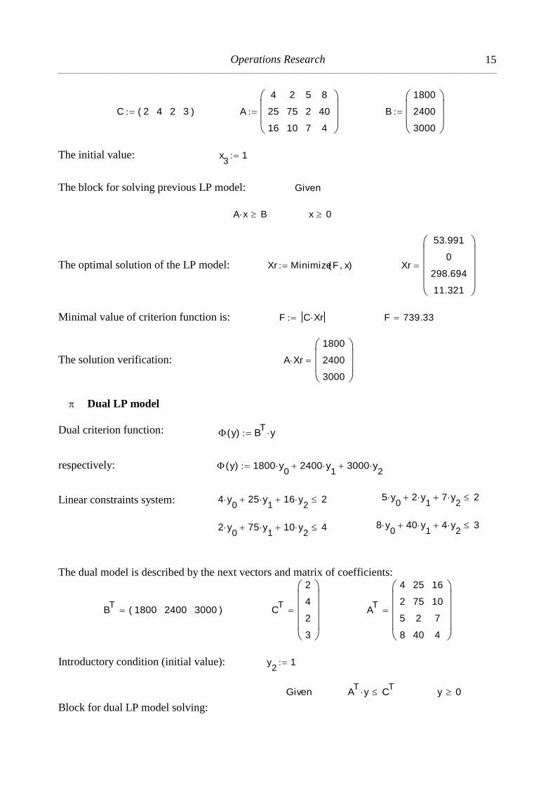
Operations Research __________________________________________________________________________________________________________
15
C 2 4 2 3( ) A
4
25
16
2
75
10
5
2
7
8
40
4
B
1800
2400
3000
The initial value: x3
1
The block for solving previous LP model: Given
A x B x 0
The optimal solution of the LP model: Xr MinimizeF x( ) Xr
53.991
0
298.694
11.321
Minimal value of criterion function is: F C Xr F 739.33
The solution verification: A Xr
1800
2400
3000
Dual LP model
Dual criterion function:
respectively: y( ) 1800 y0
2400 y1
3000 y2
Linear constraints system:
The dual model is described by the next vectors and matrix of coefficients:
BT
1800 2400 3000( ) CT
2
4
2
3
AT
4
2
5
8
25
75
2
40
16
10
7
4
Introductory condition (initial value): y2
1
Block for dual LP model solving:
y( ) BT
y
Given AT
y CT
y 0
4 y0
25 y1
16 y2
2
2 y0
75 y1
10 y2
4
5 y0
2 y1
7 y2
2
8 y0
40 y1
4 y2
3
Expositions in Mathcad __________________________________________________________________________________________________________
16
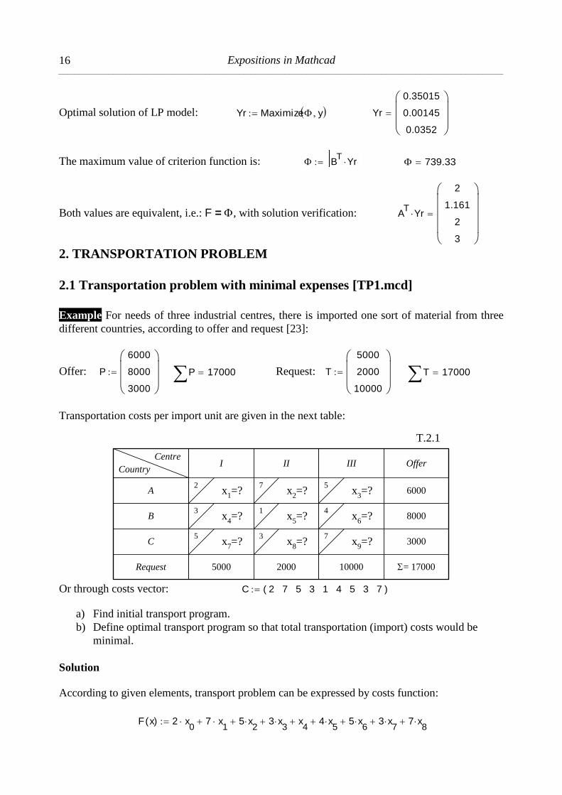
Optimal solution of LP model: Yr Maximize y Yr
0.35015
0.00145
0.0352
The maximum value of criterion function is: BT
Yr 739.33
Both values are equivalent, i.e.: F = , with solution verification: AT
Yr
2
1.161
2
3
2. TRANSPORTATION PROBLEM
2.1 Transportation problem with minimal expenses [TP1.mcd]
Example For needs of three industrial centres, there is imported one sort of material from three
different countries, according to offer and request [23]:
Offer: P
6000
8000
3000
P 17000 Request: T
5000
2000
10000
T 17000
Transportation costs per import unit are given in the next table:
T.2.1
A
I
2
II
7
III
5
B3 1 4
C5 3 7
Request 5000 2000 10000
6000
Offer
8000
3000
= 17000
Centre
Country
x1=?
x4=?
x7=?
x2=?
x5=?
x8=?
x3=?
x6=?
x9=?
Or through costs vector: C 2 7 5 3 1 4 5 3 7( )
a) Find initial transport program.
b) Define optimal transport program so that total transportation (import) costs would be
minimal.
Solution
According to given elements, transport problem can be expressed by costs function:
F x( ) 2 x
0 7 x
1 5 x
2 3 x
3 x
4 4 x
5 5 x
6 3 x
7 7 x
8

Operations Research __________________________________________________________________________________________________________
17
And coefficients matrix and constraints vector on the basis of equations system:
M
1
0
0
1
0
0
1
0
0
0
1
0
1
0
0
0
0
1
0
1
0
1
0
0
0
1
0
0
1
0
0
1
0
0
0
1
0
0
1
1
0
0
0
0
1
0
1
0
0
0
1
0
0
1
V stack P T( ) V
6000
8000
3000
5000
2000
10000
As total of offers is equal to total of requests, this problem is of closed type:
P T 1
(true)
One initial solution value of one (last) variable: x8
0
Block for solving linear programming model: Given
Linear equations system: M x V x 0
Optimal quantities of transport quantities X:
X MinimizeF x( ) X
5000
0
1000
0
0
8000
0
2000
1000
Minimum system costs: Tr C Xr Tr 60000
Values of optimal transport:
X0
X3
X6
X1
X4
X7
X2
X5
X8
5000
0
0
0
0
2000
1000
8000
1000

Expositions in Mathcad __________________________________________________________________________________________________________
18
LP solution verifikation: M X
6000
8000
3000
5000
2000
10000
2.2 Transport task with minimal expenses [TP2.mcd]
Example For needs of three business centres they import one sort of material from three various
regions according to offer and request. Transport expenses per import unit are given in the next
table.
T.2.2
R1 (25)
C1 (17)
10
C2
(21)
8
C3
(41)
9
R2 (32)
5 6 4
R3 (40)
9 7 6
Centre
Region
x1=?
x6=?
x11
=?
x2=?
x7=?
x12
=?
x3=?
x8=?
x13
=?
C4 (14)
6
3
4
x4=?
x9=?
x14
=?
C5 (24)
5
8
3
x5=?
x10
=?
x15
=?
R4 (20)
14 10 8x
16=? x
17=? x
18=?
8x
19=?
8x
20=?
a) Find initial transport program.
b) Determine optimal transport program, so that total transport expenses would be minimal.
Prices vector is formed on the basis of Matrix tool palete, through direct input of data:
C 10 8 9 6 5 5 6 4 3 8 9 7 6 4 3 14 10 8 8 8( )
According to given elements, transport problem can be expressed in the form of expenses
function (criterion):
ORIGIN 1 n 1 20 F x( )
n
CT
n xn
With adequate matrix of coefficients and constraints vector in view of equations system. The
matrix of coefficients for constraint per region capacity is:
P
1
0
0
0
1
0
0
0
1
0
0
0
1
0
0
0
1
0
0
0
0
1
0
0
0
1
0
0
0
1
0
0
0
1
0
0
0
1
0
0
0
0
1
0
0
0
1
0
0
0
1
0
0
0
1
0
0
0
1
0
0
0
0
1
0
0
0
1
0
0
0
1
0
0
0
1
0
0
0
1

Operations Research __________________________________________________________________________________________________________
19
Matrix of coefficients for constraint per centre capacity is:
S
1
0
0
0
0
0
1
0
0
0
0
0
1
0
0
0
0
0
1
0
0
0
0
0
1
1
0
0
0
0
0
1
0
0
0
0
0
1
0
0
0
0
0
1
0
0
0
0
0
1
1
0
0
0
0
0
1
0
0
0
0
0
1
0
0
0
0
0
1
0
0
0
0
0
1
1
0
0
0
0
0
1
0
0
0
0
0
1
0
0
0
0
0
1
0
0
0
0
0
1
We get complete matrix as a connected serie: A stack P S( )
A
1 2 3 4 5 6 7 8 9 10 11 12 13 14 15 16 17 18 19 20
1
2
3
4
5
6
7
8
9
1 1 1 1 1 0 0 0 0 0 0 0 0 0 0 0 0 0 0 0
0 0 0 0 0 1 1 1 1 1 0 0 0 0 0 0 0 0 0 0
0 0 0 0 0 0 0 0 0 0 1 1 1 1 1 0 0 0 0 0
0 0 0 0 0 0 0 0 0 0 0 0 0 0 0 1 1 1 1 1
1 0 0 0 0 1 0 0 0 0 1 0 0 0 0 1 0 0 0 0
0 1 0 0 0 0 1 0 0 0 0 1 0 0 0 0 1 0 0 0
0 0 1 0 0 0 0 1 0 0 0 0 1 0 0 0 0 1 0 0
0 0 0 1 0 0 0 0 1 0 0 0 0 1 0 0 0 0 1 0
0 0 0 0 1 0 0 0 0 1 0 0 0 0 1 0 0 0 0 1
The constraints vector in regions and centres is: B
25
32
40
20
17
21
41
14
24
One initial value (of the last member): x
200
Block for solving linear programming model: Given Linear equations system: A x B x 0 Optimal transport quantities: X MinimizeF x( )
XT
0 21 0 0 4 17 0 15 0 0 0 0 6 14 20 0 0 20 0 0( )
Minimal transport expenses are: T C X T 645
Expositions in Mathcad __________________________________________________________________________________________________________
20
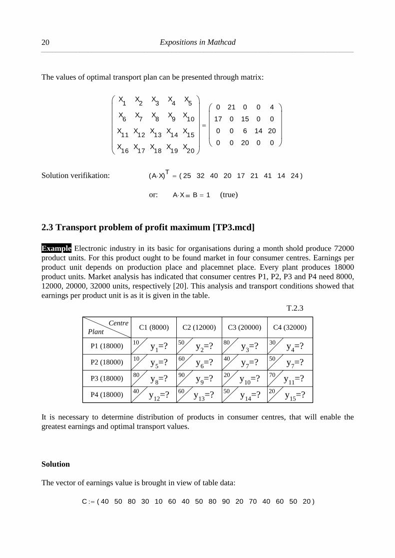
The values of optimal transport plan can be presented through matrix:
X
1
X6
X11
X16
X2
X7
X12
X17
X3
X8
X13
X18
X4
X9
X14
X19
X5
X10
X15
X20
0
17
0
0
21
0
0
0
0
15
6
20
0
0
14
0
4
0
20
0
Solution verifikation: A X( )T
25 32 40 20 17 21 41 14 24( )
or: A X B 1 (true)
2.3 Transport problem of profit maximum [TP3.mcd]
Example Electronic industry in its basic for organisations during a month shold produce 72000
product units. For this product ought to be found market in four consumer centres. Earnings per
product unit depends on production place and placemnet place. Every plant produces 18000
product units. Market analysis has indicated that consumer centres P1, P2, P3 and P4 need 8000,
12000, 20000, 32000 units, respectively [20]. This analysis and transport conditions showed that
earnings per product unit is as it is given in the table.
T.2.3
P1 (18000)
C1 (8000)
10
P2 (18000)10
P3 (18000)80
Centre
Plant
y1=?
y5=?
y8=?
P4 (18000)40
y12
=?
C2 (12000)
50
60
90
y2=?
y6=?
y9=?
60y
13=?
C3 (20000)
80
40
20
y3=?
y7=?
y10
=?
50y
14=?
C4 (32000)
30
50
70
y4=?
y7=?
y11
=?
20y
15=?
It is necessary to determine distribution of products in consumer centres, that will enable the
greatest earnings and optimal transport values.
Solution
The vector of earnings value is brought in view of table data:
C 40 50 80 30 10 60 40 50 80 90 20 70 40 60 50 20( )

Operations Research __________________________________________________________________________________________________________
21
According to given elements, transport problem can be expressed in the formof profit function:
n 0 15 D y( )
n
CT
n yn
And appropriate constraints as linear equations:
y0 y1 y3 y4 0 0 0 0 0 0 0 0 0 0 0 0 18000
0 0 0 0 y5 y6 y7 y8 0 0 0 0 0 0 0 0 18000
0 0 0 0 0 0 0 0 y9 y10 y11 y12 0 0 0 0 18000
0 0 0 0 0 0 0 0 0 0 0 0 y12 y13 y14 y15 18000
y0 0 0 0 y4 0 0 0 y8 0 0 0 y12 0 0 0 8000
0 y1 0 0 0 y5 0 0 0 y9 0 0 0 y13 0 0 12000
0 0 y2 0 0 0 y6 0 0 0 y10 0 0 0 y14 0 20000
0 0 0 y3 0 0 0 y7 0 0 0 y11 0 0 0 y15 32000
Advice Forming the previous system of constraints equations is not indispensably for solving
transport problem, in contrast to bringing in the next expressions that refer to the vectors C and B
and the matrix A.
The complete matrix of coefficients is formed by opening and filling in blank table. We have got
the Input Table through the dialoyue of Componene Wizard from the menu Insert
Componenet. The reason for table forming is that we can not form a matrix with more than 100
elements through the Insert Matrix procedure from the toolbar Matrix.
A
0 1 2 3 4 5 6 7 8 9 10 11 12 13 14 15
0
1
2
3
4
5
6
7
1 1 1 1 0 0 0 0 0 0 0 0 0 0 0 0
0 0 0 0 1 1 1 1 0 0 0 0 0 0 0 0
0 0 0 0 0 0 0 0 1 1 1 1 0 0 0 0
0 0 0 0 0 0 0 0 0 0 0 0 1 1 1 1
1 0 0 0 1 0 0 0 1 0 0 0 1 0 0 0
0 1 0 0 0 1 0 0 0 1 0 0 0 1 0 0
0 0 1 0 0 0 1 0 0 0 1 0 0 0 1 0
0 0 0 1 0 0 0 1 0 0 0 1 0 0 0 1
Expositions in Mathcad __________________________________________________________________________________________________________
22
Constraints vector by regions and centres: B
18000
18000
18000
18000
8000
12000
20000
32000
One initial value: y15 2
Block for solving linear programming: Given
Linear equations system: A y B y 0
Optimal quantities of transport quantities Y: Y Maximize D y( )
YT
0 0 18000 0 0 0 0 18000 4000 0 0 14000 4000 12000 2000 0( )
Maximum company profit is: Pr C Y Pr 4620000
The value of optimal transport plan, arranged as the matrix 4x4:
Y0
Y4
Y8
Y12
Y1
Y5
Y9
Y13
Y2
Y6
Y10
Y14
Y3
Y7
Y11
Y15
0
0
4000
4000
0
0
0
12000
18000
0
0
2000
0
18000
14000
0
Solution verifikation: A Y( )T
18000 18000 18000 18000 8000 12000 20000 32000( )
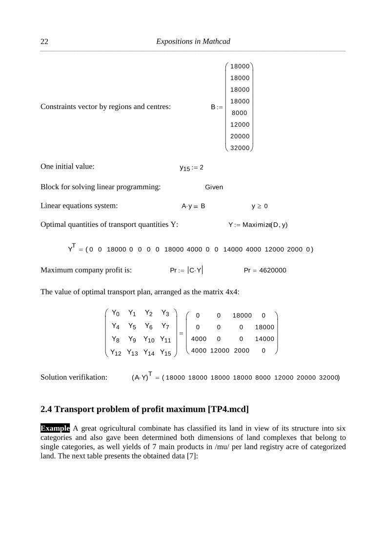
2.4 Transport problem of profit maximum [TP4.mcd]
Example A great ogricultural combinate has classified its land in view of its structure into six
categories and also gave been determined both dimensions of land complexes that belong to
single categories, as well yields of 7 main products in /mu/ per land registry acre of categorized
land. The next table presents the obtained data [7]:

Operations Research __________________________________________________________________________________________________________
23
T.2.4
iKjP Wheat Oat Oet Maize Abfalfa Potato Turnip Complex /a/
K1 12 18 5 0 20 100 60 4000
K2 8 14 3 40 10 120 0 8000
K3 18 5 5 36 16 60 0 14000
K4 16 12 0 50 4 0 140 2000
K5 4 0 8 25 0 40 230 18000
K6 5 24 0 42 18 80 200 23000
Plan /a/ 20000 16000 2000 24000 3000 1000 300069000
69000
In accordance with sowing plan it is forseen that with single sulture will be sown respectively
20000, 16000, 2000, 24000, 3000, 1000 and 3000 land registry acres (a). Which sowing plan
should be realized, if the aim is maximizing production quantity?
Solution
Vector of Prices is brought in in view of table data: ORIGIN 1
C
1 2 3 4 5 6 7 8 9 10 11 12 13 14 15
1 12 18 5 0 20 100 60 8 14 3 40 10 120 0 18
According to given elements, transport problem can be expressed in form of profit function:
n 1 42 D q( )
n
CT
n qn
And appropriate constraints in form of linear equations
Complete matrix of coefficienst is formed by opening and filling in blank of the table. We get
Input Table thruogh the dialogue of Component Wizard from the menu Insert Component.
Expositions in Mathcad __________________________________________________________________________________________________________
24
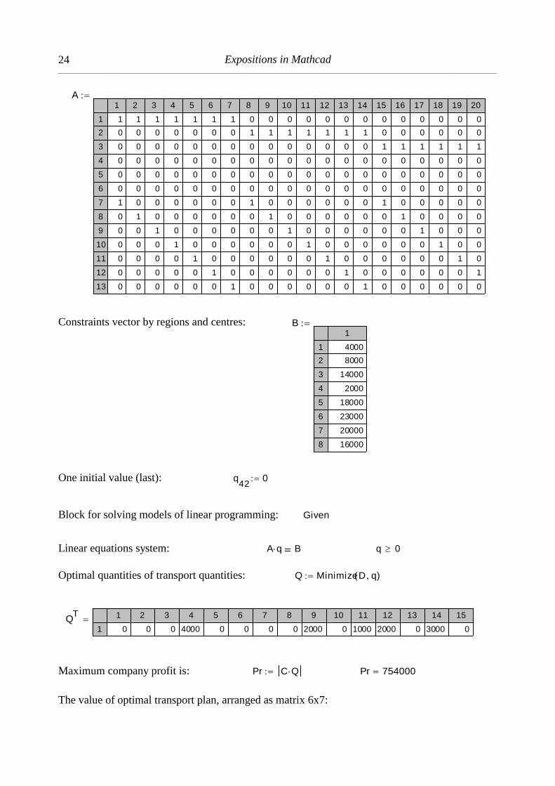
A1 2 3 4 5 6 7 8 9 10 11 12 13 14 15 16 17 18 19 20
1
2
3
4
5
6
7
8
9
10
11
12
13
1 1 1 1 1 1 1 0 0 0 0 0 0 0 0 0 0 0 0 0
0 0 0 0 0 0 0 1 1 1 1 1 1 1 0 0 0 0 0 0
0 0 0 0 0 0 0 0 0 0 0 0 0 0 1 1 1 1 1 1
0 0 0 0 0 0 0 0 0 0 0 0 0 0 0 0 0 0 0 0
0 0 0 0 0 0 0 0 0 0 0 0 0 0 0 0 0 0 0 0
0 0 0 0 0 0 0 0 0 0 0 0 0 0 0 0 0 0 0 0
1 0 0 0 0 0 0 1 0 0 0 0 0 0 1 0 0 0 0 0
0 1 0 0 0 0 0 0 1 0 0 0 0 0 0 1 0 0 0 0
0 0 1 0 0 0 0 0 0 1 0 0 0 0 0 0 1 0 0 0
0 0 0 1 0 0 0 0 0 0 1 0 0 0 0 0 0 1 0 0
0 0 0 0 1 0 0 0 0 0 0 1 0 0 0 0 0 0 1 0
0 0 0 0 0 1 0 0 0 0 0 0 1 0 0 0 0 0 0 1
0 0 0 0 0 0 1 0 0 0 0 0 0 1 0 0 0 0 0 0
Constraints vector by regions and centres: B
1
1
2
3
4
5
6
7
8
4000
8000
14000
2000
18000
23000
20000
16000
One initial value (last): q
420
Block for solving models of linear programming: Given
Linear equations system: A q B q 0
Optimal quantities of transport quantities: Q MinimizeD q( )
QT 1 2 3 4 5 6 7 8 9 10 11 12 13 14 15
1 0 0 0 4000 0 0 0 0 2000 0 1000 2000 0 3000 0
Maximum company profit is: Pr C Q Pr 754000
The value of optimal transport plan, arranged as matrix 6x7:

Operations Research __________________________________________________________________________________________________________
25
Q1
Q8
Q15
Q22
Q29
Q36
Q2
Q9
Q16
Q23
Q30
Q37
Q3
Q10
Q17
Q24
Q31
Q38
Q4
Q11
Q18
Q25
Q32
Q39
Q5
Q12
Q19
Q26
Q33
Q40
Q6
Q13
Q20
Q27
Q34
Q41
Q7
Q14
Q21
Q28
Q35
Q42
0
0
0
0
0
20000
0
2000
14000
0
0
0
0
0
0
0
0
2000
4000
1000
0
0
18000
1000
0
2000
0
1000
0
0
0
0
0
1000
0
0
0
3000
0
0
0
0
Solution verifikation:
A Q( )T 1 2 3 4 5 6 7 8 9 10 11 12 13
1 4000 8000 14000 2000 18000 23000 20000 16000 2000 24000 3000 1000 3000
Note Look at the contents of TP4_1.mcd file, where the resulting matrix is program solved.
2.5 Transport problem of minimum expenses [TP5.mcd]
Example In the following table are given goods quantities necessary to be dispatched from
forwarding stations FS, goods quantities wanted in admission stations AS, as well transport prices
from every forwarding station to every admission station.
T.2.5
OC
A1 5
B1
A2 7
A3 15
12
B2
8
4
1
B3
14
2
4
B4
6
7
36
Goods quantity
/piece/
23
29
PS
A4 6 11 5 16 12
13
B5
5
9
3
Goods quantity
/piece/13 24 15 21 =10027
Which transport plan to be realized if the objective is minimizing of total transport expenses?
Solution
Vector of prices is brought in in view of table data: ( ORIGIN 1 )
C1 2 3 4 5 6 7 8 9 10 11 12 13 14 15 16
1 5 12 1 4 13 7 8 14 6 5 15 4 2 7 9 6

Expositions in Mathcad __________________________________________________________________________________________________________
26
According to given elements, transport problem can be expressed in the form of profit function:
n 1 20 T x( )
n
CT
n xn
And adequate constraints in form of linear equations.
Complete matrix of coefficients is formed by opening and filling in blank table. We get Input
Table through the dialogue Component Wizard from the menu Insert Component.
A
1 2 3 4 5 6 7 8 9 10 11 12 13
1
2
3
4
5
6
7
8
9
1 1 1 1 1 0 0 0 0 0 0 0 0
0 0 0 0 0 1 1 1 1 1 0 0 0
0 0 0 0 0 0 0 0 0 0 1 1 1
0 0 0 0 0 0 0 0 0 0 0 0 0
1 0 0 0 0 1 0 0 0 0 1 0 0
0 1 0 0 0 0 1 0 0 0 0 1 0
0 0 1 0 0 0 0 1 0 0 0 0 1
0 0 0 1 0 0 0 0 1 0 0 0 0
0 0 0 0 1 0 0 0 0 1 0 0 0
Constraint vector by regions and centres: B1
1
2
3
4
5
6
7
8
9
36
23
29
12
13
24
15
21
27
One initial value (the last one): x
200
Block for solving linear programming model: Given
Linear equations system: A x B x 0
Optimal quantities of transport quantities q: q MinimizeT x( )
qT
5 0 10 21 0 8 0 0 0 15 0 24 5 0 0 0 0 0 0 12( )
Minimum expenses are: Tr C q Tr 392
Operations Research __________________________________________________________________________________________________________
27
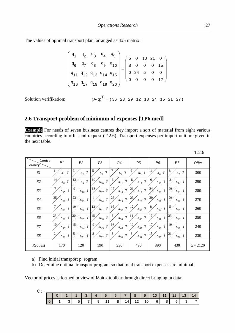
The values of optimal transport plan, arranged as 4x5 matrix:
q
1
q6
q11
q16
q2
q7
q12
q17
q3
q8
q13
q18
q4
q9
q14
q19
q5
q10
q15
q20
5
8
0
0
0
0
24
0
10
0
5
0
21
0
0
0
0
15
0
12
Solution verifikation: A q( )T
36 23 29 12 13 24 15 21 27( )
2.6 Transport problem of minimum of expenses [TP6.mcd]
Example For needs of seven business centres they import a sort of material from eight various
countries according to offer and request (T.2.6). Transport expenses per import unit are given in
the next table.
T.2.6
S1
P1
1
P2
S214
S37
Request 170
300
Offer
290
280
= 2120
Centre
Country
x1=?
x8=?
x15
=?
S435
S57
S625
x22
=?
x29
=?
x36
=?
S710
S82
x43
=?
x50
=?
P3 P4 P5 P6 P7
270
260
250
240
230
3
12
9
120
x2=?
x9=?
x16
=?
22
10
20
x23
=?
x30
=?
x37
=?
15
5
x44
=?
x51
=?
5
10
13
190
x3=?
x10
=?
x17
=?
4
13
15
x24
=?
x31
=?
x38
=?
9
8
x45
=?
x52
=?
7
6
17
330
x4=?
x11
=?
x18
=?
26
16
5
x25
=?
x32
=?
x39
=?
16
8
x46
=?
x53
=?
9
8
21
490
x5=?
x12
=?
x19
=?
23
12
11
x26
=?
x33
=?
x40
=?
12
3
x47
=?
x54
=?
11
6
24
390
x6=?
x13
=?
x20
=?
20
8
17
x27
=?
x34
=?
x41
=?
17
15
x48
=?
x55
=?
8
3
29
430
x7=?
x14
=?
x21
=?
20
5
23
x28
=?
x35
=?
x42
=?
10
21
x49
=?
x56
=?
a) Find initial transport p rogram.
b) Determine optimal transport program so that total transport expenses are minimal.
Vector of prices is formed in view of Matrix toolbar through direct bringing in data:
C0 1 2 3 4 5 6 7 8 9 10 11 12 13 14
0 1 3 5 7 9 11 8 14 12 10 6 8 6 3 7

Expositions in Mathcad __________________________________________________________________________________________________________
28
According to biven elements, transport problem can be expressed in the form of expenses
function (criterion):
ORIGIN 1 n 1 56 F x( )
n
CT
n xn
With appropriate matrix of coefficients and constraints vector in view of system of equations. The
matrix of coefficients for constraint for region capacities is:
A1 2 3 4 5 6 7 8 9 10 11 12 13 14 15 16
1
2
3
4
5
6
7
1 1 1 1 1 1 1 0 0 0 0 0 0 0 0 0
0 0 0 0 0 0 0 1 1 1 1 1 1 1 0 0
0 0 0 0 0 0 0 0 0 0 0 0 0 0 1 1
0 0 0 0 0 0 0 0 0 0 0 0 0 0 0 0
0 0 0 0 0 0 0 0 0 0 0 0 0 0 0 0
0 0 0 0 0 0 0 0 0 0 0 0 0 0 0 0
0 0 0 0 0 0 0 0 0 0 0 0 0 0 0 0
Number of elements in matrix: s last A1 1 last A
T 1
1
s 912
Constraints vector for regions and centres is: B
1
1
2
3
4
5
6
7
8
300
290
280
270
260
250
240
230
One initial value (the last one): x
560
Block for solving the model of linearn programming: Given System of linear equations: A x B x 0
Optimal transport quantities: X MinimizeF x( )
XT 1 2 3 4 5 6 7 8 9 10 11 12 13 14
1 0 10 0 80 210 0 0 0 0 0 0 0 290 0
Minimum transport expenses are: T C X T 14560

Operations Research __________________________________________________________________________________________________________
29
Values of optimal transport plan can be pressented through matrix:
X1
X8
X15
X22
X29
X36
X43
X50
X2
X9
X16
X23
X30
X37
X44
X51
X3
X10
X17
X24
X31
X38
X45
X52
X4
X11
X18
X25
X32
X39
X46
X53
X5
X12
X19
X26
X33
X40
X47
X54
X6
X13
X20
X27
X34
X41
X48
X55
X7
X14
X21
X28
X35
X42
X49
X56
0
0
170
0
0
0
0
0
10
0
110
0
0
0
0
0
0
0
0
190
0
0
0
0
80
0
0
0
0
250
0
0
210
0
0
0
0
0
50
230
0
290
0
80
20
0
0
0
0
0
0
0
240
0
190
0
Solution verification: A X( )T 1 2 3 4 5 6 7 8 9 10
1 300 290 280 270 260 250 240 230 170 120
2.7 Transport problem of minimum expenses [TP7.mcd]
Example Three mills (M1, M2 and M3) supplying with flour three bakery companies (P1, P2 and
P3). In the next month the mills can produce 750, 400 and 350 tons of flour, respectively. In the
same period the bakery companies shoul get: 75, 40 and35 tons of flour respectivey. Transport
expenses per ton of flour from mill to baker’s companies are: from the first mill 70, 30 and 60
/mu/ per Pj company respectively, from the second mill 40, 80 and 20 /mu/ per Pj company
respectively and from the third mill 10, 50 and 90 /mu/ per Pj company respectively (T.2.7).
T.2.7
M1
P1
70
P2
30
P3
60
M240 80 20
M310 50 90
Bakeries
Mills
x1=?
x4=?
x7=?
x2=?
x5=?
x8=?
x3=?
x6=?
x9=?
Capacities of
bakeries /t/
a1= 75
a2= 40
a3= 35
Capacities of
mills /t/b
1= 20 b
2= 45 b
3= 30
= 95
= 150
Find optimal transport plan, to which will suit minimal expenses.
Solution
Mathematical model is formed in order to determine open transport problem where we ought to
determine value of non-negative variables xij. Here are initial parameters:

Expositions in Mathcad __________________________________________________________________________________________________________
30
Number of rows: m 3 number of columns: n 3 (ORIGIN 1 )
Index values: i 1 3 j 1 3
Capacities in vector form: a
75
40
35
b
20
45
30
Sum of capacities: a 150 b 95 a b
And it is open transport problem. Becouse request is greater than offer, we bring in a fictitions
bakery P4 with the capacity:
b4
a b follows that: b4
0
Capacities in expanded vector are: a
75
40
35
b
20
45
30
b4
T.2.8
M1
P1
70
P2
30
P3
60
M240 80 20
M310 50 90
Bakeries
Mills
x1=?
x4=?
x7=?
x2=?
x5=?
x8=?
x3=?
x6=?
x9=?
Capacities of
bakeries /t/
a1= 75
a2= 40
a3= 35
Capacities of
mills /t/b
1= 20 b
2= 45 b
3= 30
= 95
= 150
P4
0
0
0
x4=?
x8=?
x12
=?
b4= 55
Vector of expenses value is formed through direct data input from the expanded table T.2.8:
C 70 30 60 0 40 80 20 0 10 50 90 0( )
According to the given elements, transport problem can be expressed in form of expenses
function (criterion):
k 1 n 1( ) m F x( )
k
CT
k xk
With adequate matrix of coefficients and constraints vector in view of ewuations system. The
matrix of coefficients for constraint for all capacities is:

Operations Research __________________________________________________________________________________________________________
31
Constraints vector for capacities is: B stack a b( ) B
75
40
35
20
45
30
0
One initial value (the last one): x
120
Block for solving linear programming model: Given
Linear equations system: A x B x 0
Optimal transport quantities X: X MinimizeF x( )
XT
0 45 0 30 0 0 30 10 20 0 0 15( )
Minimum transport expenses are: T C X T 2150
Values of optimal transport plan can be presented through matrix:
X1
X5
X9
X2
X6
X10
X3
X7
X11
X4
X8
X12
0
0
20
45
0
0
0
30
0
30
10
15
Arithmetical and logical solution verification: A X
75
40
35
20
45
30
55
and A X B 1 (true).

Expositions in Mathcad __________________________________________________________________________________________________________
32
3. ASSIGNMENTS PROBLEMS
3.1 Employees assignment [AP1a.mcd]
Example Production system in which are being manufactured final products from wood has
advertised an vacancy for 5 macnihe carpenters for 5 working places (planer, milling machine,
lathe, loring machine, grinder). After analyzing registration forms for the competition, all
appointed conditions have been satisfied by five candidates. In order to space workers evenly to
working places, there was organized probation [30]. Each candidate has got to process 100 same
pieces on every machine and then was found a number of good pieces that was spoilage (T.3.1).
The assignment was to dispose workers on working places, and that will provide minimal total
spoilage.
T.3.1
16
R1
R2
R3
R4
R5
3
8
33
14
9
21
23
14
21
12
2
13
19
10
6
5
10
11
15
10
5
7
11
13
Number of pointsWorkers
P1 P2 P3 P4 P5
Solution
Values vector of non-standard (bad) products: ORIGIN 1
Criterion function, as function of minimal spoilages: n 5 m 5
C
1 2 3 4 5 6 7 8 9 10 11 12 13 14 15 16 17 18 19 20 21 22 23 24 25
1 3 21 12 6 10 8 23 2 5 5 33 14 13 10 7 14 21 19 11 11 9 16 10 15 13
Criterion function, as function of minimal spoilages:
j 1 n m D x( )
1
n m
j
CT
j xj
Complete matrix of constraints is formed by opening and filling in blank table. Input table has
been got through Component wizard dialoge from Insert Component menu.
Table A size: n m( ) n m 250
Vector B size: m n 10

Operations Research __________________________________________________________________________________________________________
33
A1 2 3 4 5 6 7 8 9 10 11 12 13 14 15 16 17 18 19 20 21 22 23 24 25
1
2
3
4
5
6
7
8
9
10
1 1 1 1 1 0 0 0 0 0 0 0 0 0 0 0 0 0 0 0 0 0 0 0 0
0 0 0 0 0 1 1 1 1 1 0 0 0 0 0 0 0 0 0 0 0 0 0 0 0
0 0 0 0 0 0 0 0 0 0 1 1 1 1 1 0 0 0 0 0 0 0 0 0 0
0 0 0 0 0 0 0 0 0 0 0 0 0 0 0 1 1 1 1 1 0 0 0 0 0
0 0 0 0 0 0 0 0 0 0 0 0 0 0 0 0 0 0 0 0 1 1 1 1 1
1 0 0 0 0 1 0 0 0 0 1 0 0 0 0 1 0 0 0 0 1 0 0 0 0
0 1 0 0 0 0 1 0 0 0 0 1 0 0 0 0 1 0 0 0 0 1 0 0 0
0 0 1 0 0 0 0 1 0 0 0 0 1 0 0 0 0 1 0 0 0 0 1 0 0
0 0 0 1 0 0 0 0 1 0 0 0 0 1 0 0 0 0 1 0 0 0 0 1 0
0 0 0 0 1 0 0 0 0 1 0 0 0 0 1 0 0 0 0 1 0 0 0 0 1
Constraints vector that defines possibility that only one worker can work at one machine and that
only one work can be assigned to one worker:
B
1
1
1
1
1
1
1
1
1
1
One initial value (the last one): x25
0
Block for solving linear programming model: Given
Linear equations system: A x B x 0
Optimal arrangement of work: X MinimizeD x( )
XT 1 2 3 4 5 6 7 8 9 10 11 12 13 14 15 16 17 18 19 20 21 22 23 24 25
1 1 0 0 0 0 0 0 1 0 0 0 0 0 0 1 0 0 0 1 0 0 1 0 0 0
Optimal plan values of work arrangement, as the matrix 5x5:
Minimal total numeber of spoilages: S C X S 39

Expositions in Mathcad __________________________________________________________________________________________________________
34
X1
X6
X11
X16
X21
X2
X7
X12
X17
X22
X3
X8
X13
X18
X23
X4
X9
X14
X19
X24
X5
X10
X15
X20
X25
1
0
0
0
0
0
0
0
0
1
0
1
0
0
0
0
0
0
1
0
0
0
1
0
0
Solution verification: A X( )T
1 1 1 1 1 1 1 1 1 1( )
Conclusion On the basis of optimal solution we state that the first job should be done to the
first worker, the second to the fifth, the fhird to the second, the fourth to the fourth and the fifth to
dhe fhird. Such arrangement of jobs will show the minimum number of spoiled products of 39
pieces.
3.2 Arrangement of jobs [AP2a.mcd]
Example In production system where are made final wood products, aught to be disposed 5
workers at five working places. While the competition was finished, all assigned conditions
satisfied 5 candidates. In order to space workers at working places, there was organized test for
their vocational capabilities in view of several criterions [25]. Vocational capability was
expressed by summary number of won points, given in T.3.2.
T.3.2
R1
R2
R3
R4
R5
10
20
25
18
10
20
30
20
15
20
8
10
20
15
30
18
15
30
20
30
12
17
16
22
20
Number of pointsWorkers
P1 P2 P3 P4 P5
The assignment is to dispose workers at working places which will provide that total efficiency,
expressed through number of points, will be maximal.
Solution
Vector of points value: (ORIGIN 1 )
C
1 2 3 4 5 6 7 8 9 10 11 12 13 14 15 16 17 18 19 20 21 22 23 24 25
1 10 20 8 18 12 20 30 10 15 17 25 20 20 30 16 18 15 15 20 22 10 20 30 30 20
Criterion function, as function of maximal points: n 5 m 5

Operations Research __________________________________________________________________________________________________________
35
j 1 25 D x( )
j
CT
j xj
Complete matrix of constraints is formed by opening and filling in blank table. Input table has
been got through Component wizard dialoge from Insert – Component menu.
The size of A table: n m( ) n m 250 vector B size: m n 10
A1 2 3 4 5 6 7 8 9 10 11 12 13 14 15 16 17 18 19 20 21 22 23 24 25
1
2
3
4
5
6
7
8
9
10
1 1 1 1 1 0 0 0 0 0 0 0 0 0 0 0 0 0 0 0 0 0 0 0 0
0 0 0 0 0 1 1 1 1 1 0 0 0 0 0 0 0 0 0 0 0 0 0 0 0
0 0 0 0 0 0 0 0 0 0 1 1 1 1 1 0 0 0 0 0 0 0 0 0 0
0 0 0 0 0 0 0 0 0 0 0 0 0 0 0 1 1 1 1 1 0 0 0 0 0
0 0 0 0 0 0 0 0 0 0 0 0 0 0 0 0 0 0 0 0 1 1 1 1 1
1 0 0 0 0 1 0 0 0 0 1 0 0 0 0 1 0 0 0 0 1 0 0 0 0
0 1 0 0 0 0 1 0 0 0 0 1 0 0 0 0 1 0 0 0 0 1 0 0 0
0 0 1 0 0 0 0 1 0 0 0 0 1 0 0 0 0 1 0 0 0 0 1 0 0
0 0 0 1 0 0 0 0 1 0 0 0 0 1 0 0 0 0 1 0 0 0 0 1 0
0 0 0 0 1 0 0 0 0 1 0 0 0 0 1 0 0 0 0 1 0 0 0 0 1
The constraints vector that defines the possibility that only one worker can work at only one
machine, and that only one job can be given to one worker:
B
1
1
1
1
1
1
1
1
1
1
Block for solving linear programming model: Given
Linear equations system: A x B x 0
Optimal works disposition: X MaximizeD x( )
XT 1 2 3 4 5 6 7 8 9 10 11 12 13 14 15 16 17 18 19 20 21 22 23 24 25
1 0 0 0 1 0 0 1 0 0 0 1 0 0 0 0 0 0 0 0 1 0 0 1 0 0

Expositions in Mathcad __________________________________________________________________________________________________________
36
Maximum value of criterion function is: S C X S 125
The value of optimal arrangement of jobs, arranged as 5x5 matrix:
X1
X6
X11
X16
X21
X2
X7
X12
X17
X22
X3
X8
X13
X18
X23
X4
X9
X14
X19
X24
X5
X10
X15
X20
X25
0
0
1
0
0
0
1
0
0
0
0
0
0
0
1
1
0
0
0
0
0
0
0
1
0
Solution verifikation: A X( )T
1 1 1 1 1 1 1 1 1 1( )
Conclusion In view of optimal solution it is stated that the fourth job ought to be given to the
first worker, the second one to the second worker, the third to the first, the fourth to the fifth and
the fifth to the fourth. Such job disposition will give the greated value of the criterion function,
125 points.
3.3 Job disposition [AP3a_2.mcd]
Example Working organisation ought to open foru new working places and for them was
advertised vacancy [30]. There were five candidates in narrower selection. Their vocational
abilities for doing jobs were tested. The number of won points was given in the table T.3.3.
T.3.3
R1
R2
R3
R4
R5
5
4
8
2
6
M1
6
6
6
4
10
M2
5
4
7
4
9
M3
1
1
6
4
4
M4
Work places
Machines
How ought to dispose workers at working places, so that whole efficency would be maximum?
Which worker will not be admitted?
Solution
Previosly defined assignment problem has been opened. After adding one fictitious working
place, we get the table T.4.4, and iti is condititon for forming square matrix 5x5 and apparently
closed assignment problem.

Operations Research __________________________________________________________________________________________________________
37
T.3.4
R1
R2
R3
R4
R5
5
4
8
2
6
M1
6
6
6
4
10
M2
5
4
7
4
9
M3
1
1
6
4
4
M4
Work places
Machines
0
0
0
0
0
M5
Vector of points value: (ORIGIN 1 )
C
1 2 3 4 5 6 7 8 9 10 11 12 13 14 15 16 17 18 19 20 21 22 23 24 25
1 5 6 5 1 0 4 6 4 1 0 8 6 7 6 0 2 4 4 4 0 6 10 9 4 0
Criterion function, as function of maximal points: n 5 m 5
j 1 n m D x( )
j
CT
j xj
Complete matrix of constraints is formed by opening and filling in blank table. Input table has
been got through Component Wizard dialoge from Insert Component menu.
Table A size: n m( ) n m 250 vector B size: m n 10
A
1 2 3 4 5 6 7 8 9 10 11 12 13 14 15 16 17 18 19 20 21 22 23 24 25
1
2
3
4
5
6
7
8
9
10
1 1 1 1 1 0 0 0 0 0 0 0 0 0 0 0 0 0 0 0 0 0 0 0 0
0 0 0 0 0 1 1 1 1 1 0 0 0 0 0 0 0 0 0 0 0 0 0 0 0
0 0 0 0 0 0 0 0 0 0 1 1 1 1 1 0 0 0 0 0 0 0 0 0 0
0 0 0 0 0 0 0 0 0 0 0 0 0 0 0 1 1 1 1 1 0 0 0 0 0
0 0 0 0 0 0 0 0 0 0 0 0 0 0 0 0 0 0 0 0 1 1 1 1 1
1 0 0 0 0 1 0 0 0 0 1 0 0 0 0 1 0 0 0 0 1 0 0 0 0
0 1 0 0 0 0 1 0 0 0 0 1 0 0 0 0 1 0 0 0 0 1 0 0 0
0 0 1 0 0 0 0 1 0 0 0 0 1 0 0 0 0 1 0 0 0 0 1 0 0
0 0 0 1 0 0 0 0 1 0 0 0 0 1 0 0 0 0 1 0 0 0 0 1 0
0 0 0 0 1 0 0 0 0 1 0 0 0 0 1 0 0 0 0 1 0 0 0 0 1
Constraint vector that defines the possibility that only one worker can work at one machine and
that only one job can be given to one worker:
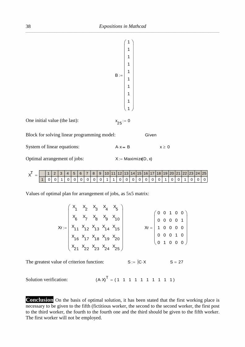
Expositions in Mathcad __________________________________________________________________________________________________________
38
B
1
1
1
1
1
1
1
1
1
1
One initial value (the last): x25
0
Block for solving linear programming model: Given
System of linear equations: A x B x 0
Optimal arrangement of jobs: X MaximizeD x( )
XT 1 2 3 4 5 6 7 8 9 10 11 12 13 14 15 16 17 18 19 20 21 22 23 24 25
1 0 0 1 0 0 0 0 0 0 1 1 0 0 0 0 0 0 0 1 0 0 1 0 0 0
Values of optimal plan for arrangement of jobs, as 5x5 matrix:
Xr
X1
X6
X11
X16
X21
X2
X7
X12
X17
X22
X3
X8
X13
X18
X23
X4
X9
X14
X19
X24
X5
X10
X15
X20
X25
Xr
0
0
1
0
0
0
0
0
0
1
1
0
0
0
0
0
0
0
1
0
0
1
0
0
0
The greatest value of criterion function: S C X S 27
Solution verification: A X( )T
1 1 1 1 1 1 1 1 1 1( )
Conclusion On the basis of optimal solution, it has been stated that the first working place is
necessary to be given to the fifth (fictitious worker, the second to the second worker, the first post
to the third worker, the fourth to the fourth one and the third should be given to the fifth worker.
The first worker will not be employed.

Operations Research __________________________________________________________________________________________________________
39
3.4 The open problem of jobs disposition [AP4a_2.mcd]
Example In an engine room of a working organization, it is necessary to perform four tasks.
These tasks can be done on six machines. Every machine can work every task, but only one at the
some time. With these tasks it is necessary to work four machines, and two to separate for other
tasks. The time for processing works on machines/hour/ is given in the table T.3.5.
T.3.5
M1
M2
M3
M4
M5
9
14
8
12
10
12
10
15
13
11
7
9
11
8
10
12
11
15
14
10
Work places
Machines
T1 T2 T3 T4
M6 11 14 12 9
How to dispose tasks on machines so the used time for performing all tasks to be as shorter as
possible?
Solution
Previously defined assignment problem is open. After adding two fictitious tasks, we get the table
T.3.6, and it is the condition for forming square matrix and apparently closed assignment
problem.
T.3.6
M1
M2
M3
M4
M5
9
14
8
12
10
12
10
15
13
11
7
9
11
8
10
12
11
15
14
10
Work places
Machines
T1 T2 T3 T4
M6 11 14 12 9
0
0
0
0
0
T5
0
0
0
0
0
0
T6
0
Value vector of points C: ( ORIGIN 1 )
C1 2 3 4 5 6 7 8 9 10 11 12 13 14 15 16 17 18 19 20 21 22 23 24 25
1 9 12 7 12 0 0 14 10 9 11 0 0 8 15 11 15 0 0 12 13 8 14 0 0 10

Expositions in Mathcad __________________________________________________________________________________________________________
40
Criterion function, as function of maximal points: n 6 m 6
j 1 n m D x( )
j
CT
j xj
Complete matrix of limit (ations) coefficients is formed by opening and filling in blank table. We
get Input Table through Component Wizard from the menu Insert Component.
A
1 2 3 4 5 6 7 8 9 10 11 12 13 14 15 16 17 18 19 20 21 22 23 24
1
2
3
4
5
6
7
8
9
10
11
12
1 1 1 1 1 1 0 0 0 0 0 0 0 0 0 0 0 0 0 0 0 0 0 0
0 0 0 0 0 0 1 1 1 1 1 1 0 0 0 0 0 0 0 0 0 0 0 0
0 0 0 0 0 0 0 0 0 0 0 0 1 1 1 1 1 1 0 0 0 0 0 0
0 0 0 0 0 0 0 0 0 0 0 0 0 0 0 0 0 0 1 1 1 1 1 1
0 0 0 0 0 0 0 0 0 0 0 0 0 0 0 0 0 0 0 0 0 0 0 0
0 0 0 0 0 0 0 0 0 0 0 0 0 0 0 0 0 0 0 0 0 0 0 0
1 0 0 0 0 0 1 0 0 0 0 0 1 0 0 0 0 0 1 0 0 0 0 0
0 1 0 0 0 0 0 1 0 0 0 0 0 1 0 0 0 0 0 1 0 0 0 0
0 0 1 0 0 0 0 0 1 0 0 0 0 0 1 0 0 0 0 0 1 0 0 0
0 0 0 1 0 0 0 0 0 1 0 0 0 0 0 1 0 0 0 0 0 1 0 0
0 0 0 0 1 0 0 0 0 0 1 0 0 0 0 0 1 0 0 0 0 0 1 0
0 0 0 0 0 1 0 0 0 0 0 1 0 0 0 0 0 1 0 0 0 0 0 1
Limit factor by which is defined that only one worker can work at one machine and that only one
job can be given to one worker.
B
1
1
2
3
4
5
1
1
1
1
1
One initial value (the last one): x36
0
Block for solving linear programming model: Given
System of linear equations: A x B x 0
Optimal disposition of jobs: X MinimizeD x( )
XT 1 2 3 4 5 6 7 8 9 10 11 12 13 14 15 16 17 18 19 20 21 22 23
1 0 0 1 0 0 0 0 1 0 0 0 0 1 0 0 0 0 0 0 0 0 0 1
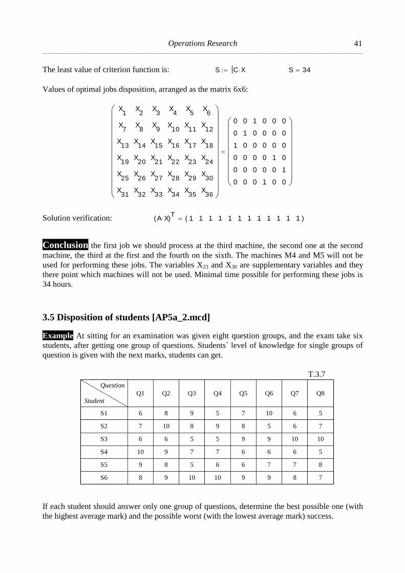
Operations Research __________________________________________________________________________________________________________
41
The least value of criterion function is: S C X S 34
Values of optimal jobs disposition, arranged as the matrix 6x6:
X1
X7
X13
X19
X25
X31
X2
X8
X14
X20
X26
X32
X3
X9
X15
X21
X27
X33
X4
X10
X16
X22
X28
X34
X5
X11
X17
X23
X29
X35
X6
X12
X18
X24
X30
X36
0
0
1
0
0
0
0
1
0
0
0
0
1
0
0
0
0
0
0
0
0
0
0
1
0
0
0
1
0
0
0
0
0
0
1
0
Solution verification: A X( )T
1 1 1 1 1 1 1 1 1 1 1 1( )
Conclusion the first job we should process at the third machine, the second one at the second
machine, the third at the first and the fourth on the sixth. The machines M4 and M5 will not be
used for performing these jobs. The variables X23 and X30 are supplementary variables and they
there point which machines will not be used. Minimal time possible for performing these jobs is
34 hours.
3.5 Disposition of students [AP5a_2.mcd]
Example At sitting for an examination was given eight question groups, and the exam take six
students, after getting one group of questions. Students` level of knowledge for single groups of
question is given with the next marks, students can get.
T.3.7
S1
S2
S3
S4
S5
6
7
6
10
9
Q1Student
Question
8
10
6
9
8
Q2
9
8
5
7
5
Q3
5
9
5
7
6
Q4
7
8
9
6
6
Q5
S6 8 9 10 10 9
10
5
9
6
7
Q6
6
6
10
6
7
Q7
5
7
10
5
8
Q8
9 8 7
If each student should answer only one group of questions, determine the best possible one (with
the highest average mark) and the possible worst (with the lowest average mark) success.
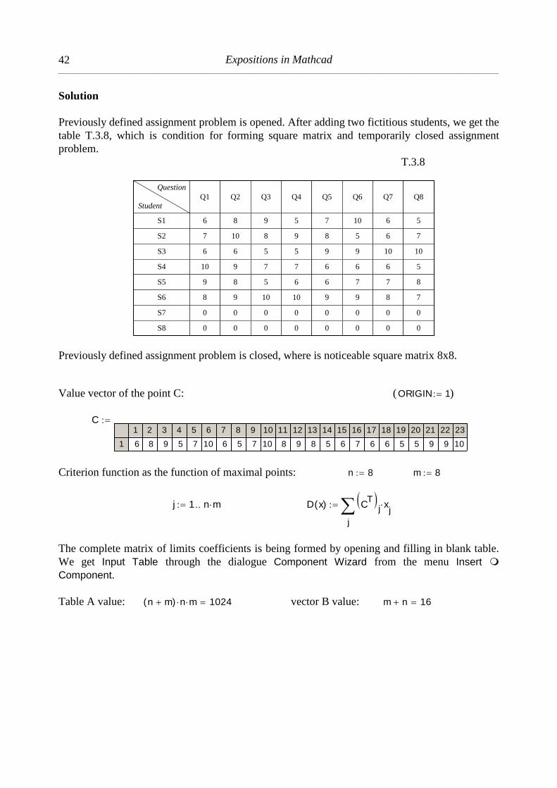
Expositions in Mathcad __________________________________________________________________________________________________________
42
Solution
Previously defined assignment problem is opened. After adding two fictitious students, we get the
table T.3.8, which is condition for forming square matrix and temporarily closed assignment
problem.
T.3.8
S1
S2
S3
S4
S5
6
7
6
10
9
Q1
8
10
6
9
8
Q2
9
8
5
7
5
Q3
5
9
5
7
6
Q4
7
8
9
6
6
Q5
S6 8 9 10 10 9
10
5
9
6
7
Q6
6
6
10
6
7
Q7
5
7
10
5
8
Q8
9 8 7
S7 0 0 0 0 0
S8 0 0 0 0 0
0 0 0
0 0 0
Student
Question
Previously defined assignment problem is closed, where is noticeable square matrix 8x8.
Value vector of the point C: (ORIGIN 1 )
C
1 2 3 4 5 6 7 8 9 10 11 12 13 14 15 16 17 18 19 20 21 22 23
1 6 8 9 5 7 10 6 5 7 10 8 9 8 5 6 7 6 6 5 5 9 9 10
Criterion function as the function of maximal points: n 8 m 8
j 1 n m D x( )
j
CT
j xj
The complete matrix of limits coefficients is being formed by opening and filling in blank table.
We get Input Table through the dialogue Component Wizard from the menu Insert
Component.
Table A value: n m( ) n m 1024 vector B value: m n 16

Operations Research __________________________________________________________________________________________________________
43
A1 2 3 4 5 6 7 8 9 10 11 12 13 14 15 16 17 18 19 20 21 22 23 24 25 26 27
1
2
3
4
5
6
1 1 1 1 1 1 1 1 0 0 0 0 0 0 0 0 0 0 0 0 0 0 0 0 0 0 0
0 0 0 0 0 0 0 0 1 1 1 1 1 1 1 1 0 0 0 0 0 0 0 0 0 0 0
0 0 0 0 0 0 0 0 0 0 0 0 0 0 0 0 1 1 1 1 1 1 1 1 0 0 0
0 0 0 0 0 0 0 0 0 0 0 0 0 0 0 0 0 0 0 0 0 0 0 0 1 1 1
0 0 0 0 0 0 0 0 0 0 0 0 0 0 0 0 0 0 0 0 0 0 0 0 0 0 0
0 0 0 0 0 0 0 0 0 0 0 0 0 0 0 0 0 0 0 0 0 0 0 0 0 0 0
Limit vector that has defined that only one worker can work at one machine and that only one job
may be disposed to one worker:
Finding the most favourable combination
One initial value (last): x64
0
Block for solving model of linear programming: Given Linear equations system: A x B x 0
Optimal distribution of jobs: X MaximizeD x( )
XT 1 2 3 4 5 6 7 8 9 10 11 12 13 14 15 16 17 18 19 20 21 22 23 24 25
1 0 0 0 0 0 1 0 0 0 1 0 0 0 0 0 0 0 0 0 0 0 0 1 0 1
Optimal plan values for jobs distribution, as the matrix 8x8:
The least value of criterion function: S C X S 58

Expositions in Mathcad __________________________________________________________________________________________________________
44
Xr
X1
X9
X17
X25
X33
X41
X49
X57
X2
X10
X18
X26
X34
X42
X50
X58
X3
X11
X19
X27
X35
X43
X51
X59
X4
X12
X20
X28
X36
X44
X52
X60
X5
X13
X21
X29
X37
X45
X53
X61
X6
X14
X22
X30
X38
X46
X54
X62
X7
X15
X23
X31
X39
X47
X55
X63
X8
X16
X24
X32
X40
X48
X56
X64
Xr
0
0
0
1
0
0
0
0
0
1
0
0
0
0
0
0
0
0
0
0
0
1
0
0
0
0
0
0
0
0
0
1
0
0
0
0
0
0
1
0
1
0
0
0
0
0
0
0
0
0
1
0
0
0
0
0
0
0
0
0
1
0
0
0
Solution verification: A X( )T
1 1 1 1 1 1 1 1 1 1 1 1 1 1 1 1( ) In view of optimal solution the next results are concluded concerning maximum, when there are
being combined group of questions and the next structure students:
T.3.9
Student
Group of question
Mark
S1
Q6
10
S2
Q2
10
S3
Q7
10
S4
Q1
10
S5
Q8
8
S6
Q4
10
The highest average mark is: S
m 29.667
One initial value (last): x64
0
Block for solving linear programming models: Given
Linear equations system: A x B x 0
Optimal disposition of jobs: X MinimizeD x( )
XT 1 2 3 4 5 6 7 8 9 10 11 12 13 14 15 16 17 18 19 20 21 22 23 24
1 0 0 0 0 0 0 0 1 0 0 0 0 0 1 0 0 0 0 0 1 0 0 0 0
The values of optimal plan for jobs disposition, as the matrix 8x8:
The least value of criterion function: S C X S 34
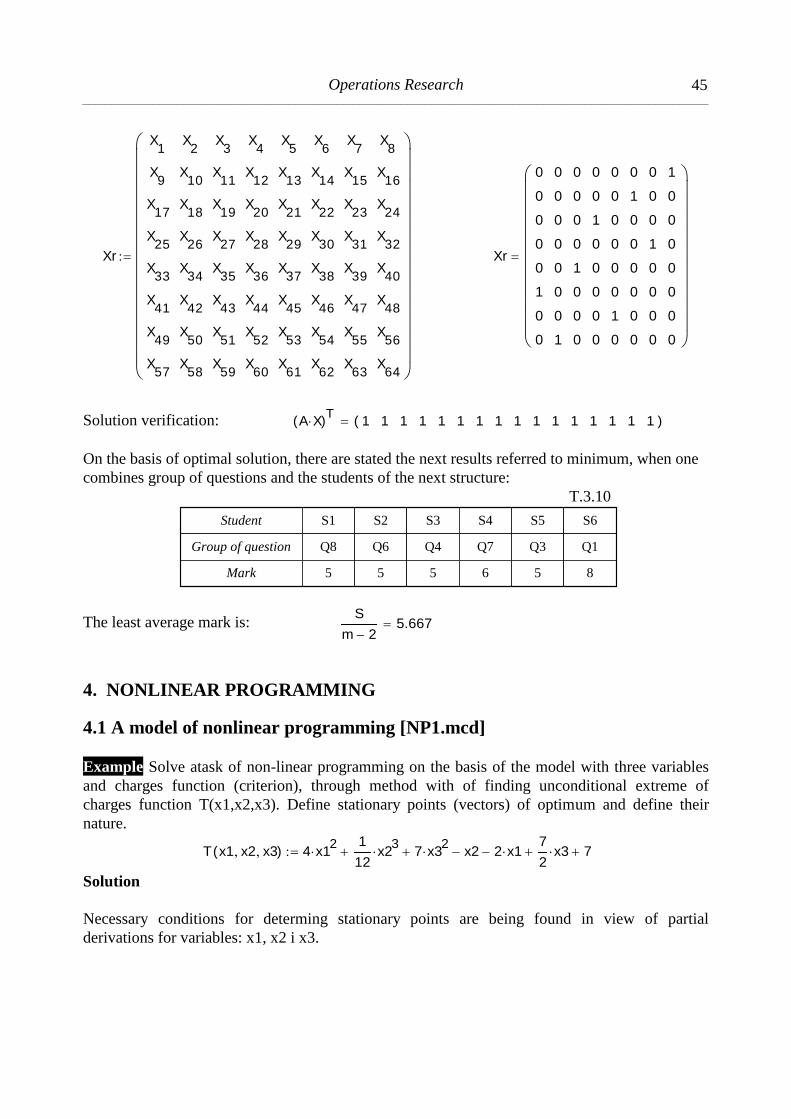
Operations Research __________________________________________________________________________________________________________
45
Xr
X1
X9
X17
X25
X33
X41
X49
X57
X2
X10
X18
X26
X34
X42
X50
X58
X3
X11
X19
X27
X35
X43
X51
X59
X4
X12
X20
X28
X36
X44
X52
X60
X5
X13
X21
X29
X37
X45
X53
X61
X6
X14
X22
X30
X38
X46
X54
X62
X7
X15
X23
X31
X39
X47
X55
X63
X8
X16
X24
X32
X40
X48
X56
X64
Xr
0
0
0
0
0
1
0
0
0
0
0
0
0
0
0
1
0
0
0
0
1
0
0
0
0
0
1
0
0
0
0
0
0
0
0
0
0
0
1
0
0
1
0
0
0
0
0
0
0
0
0
1
0
0
0
0
1
0
0
0
0
0
0
0
Solution verification: A X( )T
1 1 1 1 1 1 1 1 1 1 1 1 1 1 1 1( )
On the basis of optimal solution, there are stated the next results referred to minimum, when one
combines group of questions and the students of the next structure:
T.3.10
Student
Group of question
Mark
S1
Q8
5
S2
Q6
5
S3
Q4
5
S4
Q7
6
S5
Q3
5
S6
Q1
8
The least average mark is: S
m 25.667
4. NONLINEAR PROGRAMMING
4.1 A model of nonlinear programming [NP1.mcd]
Example Solve atask of non-linear programming on the basis of the model with three variables
and charges function (criterion), through method with of finding unconditional extreme of
charges function T(x1,x2,x3). Define stationary points (vectors) of optimum and define their
nature.
T x1 x2 x3( ) 4 x12
1
12x2
3 7 x3
2 x2 2 x1
7
2x3 7
Solution
Necessary conditions for determing stationary points are being found in view of partial
derivations for variables: x1, x2 i x3.

Expositions in Mathcad __________________________________________________________________________________________________________
46
x1T x1 x2 x3( )
8 x1 2
x2T x1 x2 x3( )
1
4x2
2 1
x3T x1 x2 x3( )
14 x3
7
2
For determing stationary vectors x<1> and x<2> previously found derivations are equaled with
zero:
ORIGIN 1 Given
8 x1 2 01
4x2
2 1 0 14 x3
7
2 0
MinErr x1 x2 x3( )
1
4
2
1
4
1
4
2
1
4
what can be presented by the matrix: x
1
4
2
1
4
1
4
2
1
4
In view of previous results, we find that there are two stationary function points, presented
through vectors:
x1 1
0.25 x1 2
0.25
x1
0.25
2
0.25
x2
0.25
2
0.25
x2 1
2 x2 2
2
x3 1
0.25 x3 2
0.25
By derivation of higher progression and mixed derivations of many variables, are being stated its
characteristics in environment of stationary points. These derivations can be directly arranged in
determinants for stationary points:

Operations Research __________________________________________________________________________________________________________
47
det1 x1 x2 x3( )2
x1T x1 x2 x3( )
28
det2 x1 x2 x3( )
2x1
T x1 x2 x3( )
2
x2 x1T x1 x2 x3( )
x1 x2T x1 x2 x3( )
2x2
T x1 x2 x3( )
2
4 x2
det3 x1 x2 x3( )
2x1
T x1 x2 x3( )
2
x2 x1T x1 x2 x3( )
x3 x1T x1 x2 x3( )
x1 x2T x1 x2 x3( )
2x2
T x1 x2 x3( )
2
x3 x2T x1 x2 x3( )
x1 x3T x1 x2 x3( )
x2 x3T x1 x2 x3( )
2x3
T x1 x2 x3( )
2
56 x2
Concrete values of determinants for stationary points, can be stated through substitution of values
for numerical elements of the first vector, then the second one. In view of that follow the results:
det1 x1 1
x2 1
x3 1
det2 x
1 1x2 1
x3 1
det3 x
1 1x2 1
x3 1
8
8
112
det1 x1 2
x2 2
x3 2
det2 x
1 2x2 2
x3 2
det3 x
1 2x2 2
x3 2
8
8
112
As all values are determinants (det1, det2 i det3) > 0, for x<1> here results that the function
T x1 1
x2 1
x3 1
has local minimum with numerical value:
T x1 1
x2 1
x3 1
4.979
Through similar procedure, by substitution of the vector x<2>, we are testing the amount of
criterion changes function, in this stationary point:
T x1 2
x2 2
x3 2
7.646
As: T x1 2
x2 2
x3 2
T x1 1
x2 1
x3 1
1 the solution is verified, so it comes that the
first point T x1 1
x2 1
x3 1
is global minimum of charges function.

Expositions in Mathcad __________________________________________________________________________________________________________
48
4.2 Profit maximization through nonlinear programming method [NP2.mcd]
Example On the basic of defined functions R(q) – incomes and T(q) – costs [2]:
a) Define optimal volume of sale for profit maximization.
b) State value of profit for minimal average costs.
c) Check and design on a chart functions of income, costs and profit.
d) How great is interval of great power?
Solution
Function of income: R q( ) 400 q q2
Function of costs: T q( ) 3 q2
1200
Profit is defined as difference of total incomes and total costs:
q( ) R q( ) T q( ) 400 q 4 q2
1200
The conditions achieving maximum of profit function are that the first derivation should be zero
and the second one negative:
q q( )
d
d400 8 q
2q
q( )d
d
28
Consequently, profit maximum is achieved when the volume of production (sale) is 50, so then is
realized the profit of 8800 /nj/.
q q( )
d
d0 solve q 50 50( ) 8800
Minimal average costs can present criterion for production optimization. In the concrete case they
are achieved through the next procedures:
t q( )T q( )
q t q( )
3 q2
1200 q
2
qt q( )
d
d
2simplify
2400
q3
qt q( )
d
d0 solve q
20
20
20( ) 5200
For volume of sale (production) of q=20 product units, we can realize minimal average costs, and
the profit then realized is 5200 /nj/.

Operations Research __________________________________________________________________________________________________________
49
0 50 100 150 200 250 300 350 400 4500
1 104
2 104
3 104
4 104
5 104
q( )
R q( )
T q( )
50 200
q
Fig. 4.1 The chart of functions for profit, costs and income
Points of section for the functions R(q) and T(q)
Initial value of solution: q 50
Solution of functions cross-section: Q1 root R q( ) T q( ) q( ) Q1 96.9
Verification of functions values: R Q1( )
T Q1( )
29371.247
29371.247
One should note that the first coordinates of these points are exactly also the first coordinates of
zero value of profit function.
Points of selection for the functions R(q) and P(q)
Solution of functions cross-selection: Q2 root R q( ) q( ) q Q2 20i
Verification of functions values: R Q2( )
Q2( )
400 8000i
400 8000i

Expositions in Mathcad __________________________________________________________________________________________________________
50
In relation of the two functions R(q) and P(q) we can not find real solution of cross-selection, but
only complex (imaginary). Consequently, it follows that it is impossible that profit should be
equal to incomes.
Points of section for the functions T(q) and P(q)
Solution of functions cross-selection: Q3 root T q( ) q( ) q Q3 50.33
Verification of functions value: Q3( )
T Q3( )
8799.562
8799.562
Interval of earning power is the interval for which profit is positive, or alternative field where
incomes are greater than costs:
Q( ) 400 Q 4 Q2
1200 A Q( ) coeffs Q
1200
400
4
q polyroots A( ) q3.096
96.904
q0
3.096 q1
96.904
In concrete example it is the interval [q0,q1]. In that interval company realizes its gaining
business (operations). Consequently, it is exactly the field between two zeros of profit function,
respectively the field between two points of section of total income function and total costs.
4.3 Conditions of production optimality (optimum) [NP3.mcd]
Example For the product x are given demand function x(p) and costs function C(x). Determine
production for which is being realized maximal profit and its amount.
Starting data: a1
4 b 1200 c 2 d 900
Demand function: x p( ) a p b
Costs function: C x( ) c x2
d Inverse form of demand function: p x( ) a p b x 0 solve p 4800 4 x
Or by redefinition (only change of marks, x X): p X( ) 4800 4 X
In come function is then: P X( ) X p X( ) X 4800 4 X( )
Redefinition of costs function: C X( ) 2 X2
900

Operations Research __________________________________________________________________________________________________________
51
Then profit function is defined as:
D x( ) P x( ) C x( ) simplify 4800 x 6 x2
900
Izvodna funkcija dobiti je: D x( )xD x( )
d
d4800 12 x
Solving derived equation, we get a solution xo as optimal value of production:
Given D x( ) 0 xo Find x( ) 400
So, maximal profits: D xo( ) 959100
The interval of earning power in determined from the conditions: Given D x( ) 0
Solving square equation we get solution vector:
x Find x( ) 400 5 6394 400 5 6394 xT 799.812
0.188
xr xT
The earning power is between the values:
xr0
799.812
i xr1
0.188
4.4 Utility function-optimal volume of purchase of goods [NP4.mcd]
Example For the given utility function U and budget equation D with fixed budget Do determine
optimal purchase volume (acquisition) of observed goods, so to realize maximal utility [23].
Starting parameters: p1 45 p2 24
Values of fixed budget Do: Do 680
Utility function: U x y( ) 85 x y2
Lagrange’s equation: G x y U x y( ) Do D x y( )( ) Partial deviations for x, y and :

Expositions in Mathcad __________________________________________________________________________________________________________
52
G1 x y x
G x y
G1 x y 85 y
2 45
G2 x y y
G x y
G2 x y 170 x y 24
G3 x y
G x y
G3 x y 680 45 x 24 y
Other partial derivations are:
F11 x y 2
xG x y
2 F11 x y 0
F12 x y x y
G x y
F12 x y 170 y
F21 x y y x
G x y
F21 x y 170 y
F22 x y 2
yG x y
2 F22 x y 170 x
Determing optimal value of goods purchase. For initial values is formed block for calculation:
x 2 y 2 1 Given
G1 x y 0 G2 x y 0 G3 x y 0
Optimal values of the two variables (xo, yo) make:
xo
yo
o
Find x y xo
yo
5.037
18.889
With this maximal value of utility function is: U xo yo( ) 152759.031
Values of partial derivations for optimal values:
F11 xo yo 0 F12 xo yo 3211.111
F21 xo yo 3211.111 F22 xo yo 856.296 The condition that verifies maximal values of utility function is expressed by positive value of
Hesian determinant.

Operations Research __________________________________________________________________________________________________________
53
H
F11 xo yo
F21 xo yo
p1
F12 xo yo
F22 xo yo
p2
p1
p2
0
H 5202000 H 0 1 (affirmatively)
From where is confirmed that Hesian determinant is positive.
4.5 Optimization of enzyme product [NP5.mcd]
Example Optimization of models for biological processes can be observed from many views.
First, that during evolution has happened significant bio-chemical changes. Now researchers
should determine different metabolic pathways and genetic models caused by them. The second is
the method of artificial improvement of these systems, because of different demands as insulin
production out of DNA resources, before it is isolated from animal glands and the like. Taking
this in consideration, researchers have developed mathematical program for ethyl-alcohol
optimization, glycerin (e) (propan-triol) and production of carbohydrates in Saccharomyces
cerevisiae in conditions of broken of cell culture in ph4.5.
Starting parameters connected with chemical compounds, are given in the next table:
T.4.1
Chemical compound Concentration Concentration Concentration
Internal glucose x1 0.034 Phosphofructokinase x8 31.7
Glucose-6-phosphate x2 1.01 Glyceraldehyde-3-phosphate
dehydrogenase x9 49.9
Fructose-1,6-diphosphate x3 9.144 Pyruvate kinase x10 3440
Phospheoenolpyruvate x4 0.0095 Polysaccharide production x11 14.31
Adenozin-tri-fosfat (ATP) x5 1.1278 Glycerol production: x12 203
Glucose uptake x6 19.7 ATPase x13 25.1
Enzim hexokinase x7 68.5 NAD/NADH ratio x14 0.042
Solution

Expositions in Mathcad __________________________________________________________________________________________________________
54
Exact model with limit functions:
Given
Sugar transport: x1 0.8122 x20.2344
x6 2.8632 x10.7464
x50.0243
x7
Hexokinase enzyme:
x2 2.8632 x1 x50.0243
x7 0.5236 x20.735
x50.394
x80.999
x110.001
The kind of enzyme whose reaction causes compound breakdown (Phospofructokinase reaction).
x3 0.5232 x20.7318
x50.3941
x8
Enzim Pyruvatekinase:
x4 0.022 x30.6159
x50.1308
x9 x140.6088
0.0945 x30.05
x40.533
x50.0822
x10
ATP (Adenozin-tri- phosphate):
x5 3.2097 x10.198
x20.196
x50.372
x70.265
x80.265
x110.002
x130.47
0.0913 x30.333
x40.266
x50.024
x90.5
x100.5
x140.304
Finding variables for constant state of concentration:
K Find x1 x2 x3 x4 x5 x6 x7 x8 x9 x10 x11 x12 x13 x14( )
Solution of equations system:
KT
0.04 0.8 8.45 0.01 1.24 24.47 80.46 20.76 50.24 3367.16 14.31 203 24.97 0.04( )
The hypothesis is that optimization of ethyl-alcohol production a real function and it is necessary
to invent such a value, that the flowing through would be maximal one.
C x1 x2 x3 x4 x5 x6 x7 x8 x9 x10 x11 x12 x13 x14( ) 0.0945 x3.05
x4.533
x5.0822
x10
The values of chemical compounds will be here initial for (non) equations of a constant state.
According to Clifford (?) we can decide how much is to each enzyme allowed to change itself
(with supposition that it can be physiologically and bio-technically realized). In terms of it are set
limits to metabolite concentration:
Limit functions:
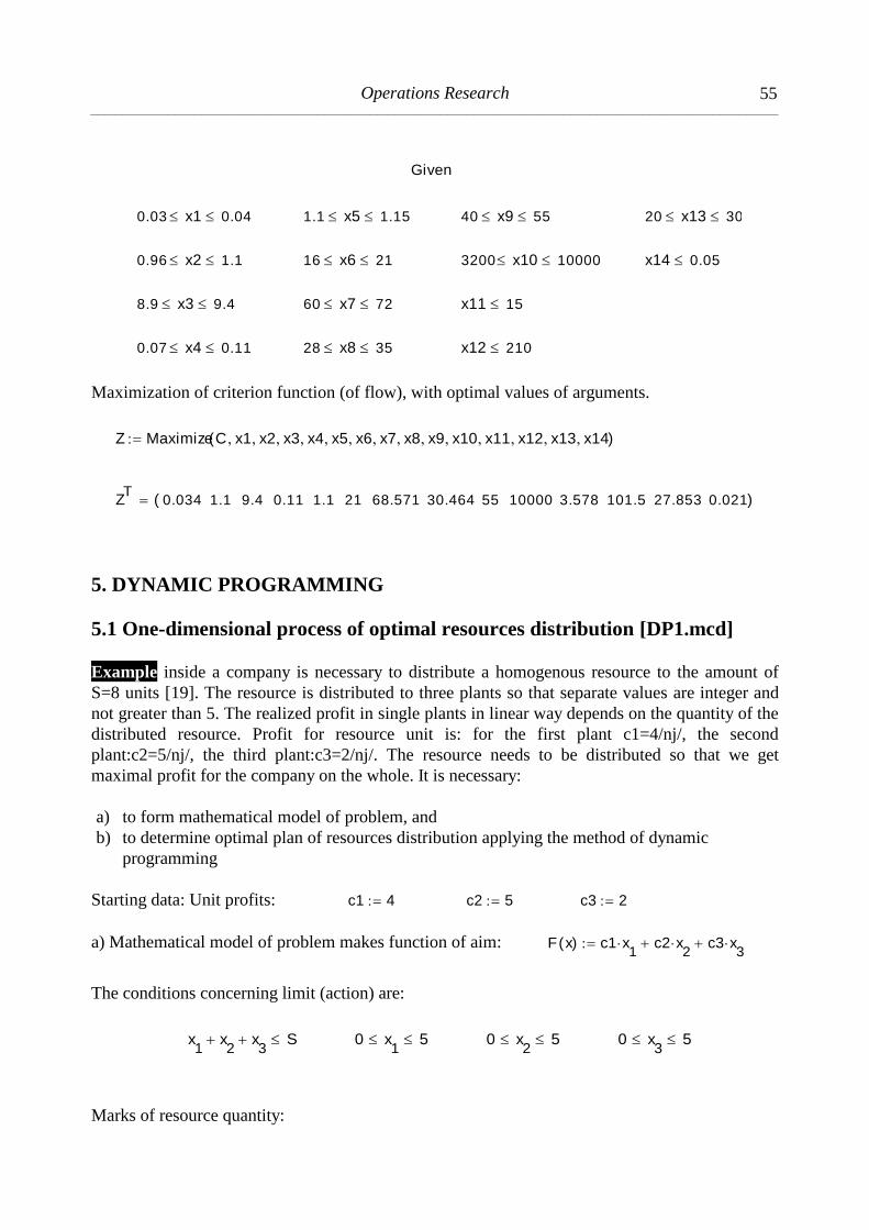
Operations Research __________________________________________________________________________________________________________
55
Given
0.03 x1 0.04 1.1 x5 1.15 40 x9 55 20 x13 30
0.96 x2 1.1 16 x6 21 3200 x10 10000 x14 0.05
8.9 x3 9.4 60 x7 72 x11 15
0.07 x4 0.11 28 x8 35 x12 210 Maximization of criterion function (of flow), with optimal values of arguments.
Z Maximize C x1 x2 x3 x4 x5 x6 x7 x8 x9 x10 x11 x12 x13 x14( )
ZT
0.034 1.1 9.4 0.11 1.1 21 68.571 30.464 55 10000 3.578 101.5 27.853 0.021( )
5. DYNAMIC PROGRAMMING
5.1 One-dimensional process of optimal resources distribution [DP1.mcd]
Example inside a company is necessary to distribute a homogenous resource to the amount of
S=8 units [19]. The resource is distributed to three plants so that separate values are integer and
not greater than 5. The realized profit in single plants in linear way depends on the quantity of the
distributed resource. Profit for resource unit is: for the first plant c1=4/nj/, the second
plant:c2=5/nj/, the third plant:c3=2/nj/. The resource needs to be distributed so that we get
maximal profit for the company on the whole. It is necessary:
a) to form mathematical model of problem, and
b) to determine optimal plan of resources distribution applying the method of dynamic
programming
Starting data: Unit profits: c1 4 c2 5 c3 2
a) Mathematical model of problem makes function of aim: F x( ) c1 x1
c2 x2
c3 x3
The conditions concerning limit (action) are:
x1
x2
x3
S 0 x1
5 0 x2
5 0 x3
5
Marks of resource quantity:

Expositions in Mathcad __________________________________________________________________________________________________________
56
x30 0 x31 1 x32 2 x33 3 x34 4 x35 5
Recurrent relation of direct profit from the distribution for the first resource:
S 0 8 f1S
if c1 S c1 x35 c1 x35 c1 S f1S
0
4
8
12
16
20
20
20
20
max f1( ) 20
Recurrent relation of direct profit from the distribution for the second resource:
S 0 x2 0 S f20x2
c2 x2 f1S x2
f20x2
0
max f20( ) 0
S 1 x2 0 S f21x2
c2 x2 f1S x2
f21x2
4
5
max f21( ) 5
S 2 x2 0 S f22x2
c2 x2 f1S x2
f22x2
8
9
10
max f22( ) 10
S 3 x2 0 S f23x2
c2 x2 f1S x2
f23x2
12
13
14
15
max f23( ) 15

Operations Research __________________________________________________________________________________________________________
57
S 4 x2 0 S f24x2
c2 x2 f1S x2
f24x2
16
17
18
19
20
max f24( ) 20
S 5 x2 0 S f25x2
c2 x2 f1S x2
f25x2
20
21
22
23
24
25
max f25( ) 25
S 6 x2 0 S 1 f26x2
c2 x2 f1S x2
f26x2
20
25
26
27
28
29
max f26( ) 29
S 7 x2 0 S 2 f27x2
c2 x2 f1S x2
f27x2
20
25
30
31
32
33
max f27( ) 33
S 8 x2 0 S 3 f28x2
c2 x2 f1S x2
f28x2
20
25
30
35
36
37
max f28( ) 37
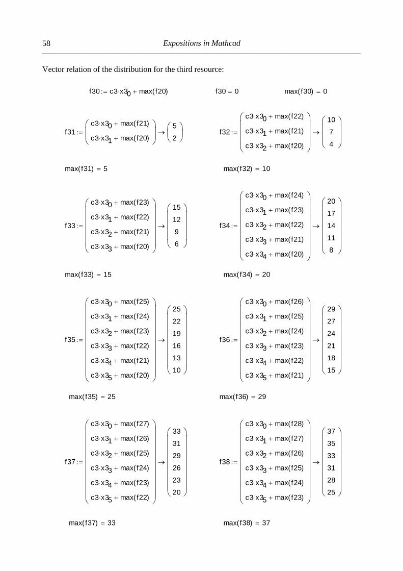
Expositions in Mathcad __________________________________________________________________________________________________________
58
Vector relation of the distribution for the third resource:
max f38( ) 37max f37( ) 33
f38
c3 x30 max f28( )
c3 x31 max f27( )
c3 x32 max f26( )
c3 x33 max f25( )
c3 x34 max f24( )
c3 x35 max f23( )
37
35
33
31
28
25
f37
c3 x30 max f27( )
c3 x31 max f26( )
c3 x32 max f25( )
c3 x33 max f24( )
c3 x34 max f23( )
c3 x35 max f22( )
33
31
29
26
23
20
max f36( ) 29max f35( ) 25
f36
c3 x30 max f26( )
c3 x31 max f25( )
c3 x32 max f24( )
c3 x33 max f23( )
c3 x34 max f22( )
c3 x35 max f21( )
29
27
24
21
18
15
f35
c3 x30 max f25( )
c3 x31 max f24( )
c3 x32 max f23( )
c3 x33 max f22( )
c3 x34 max f21( )
c3 x35 max f20( )
25
22
19
16
13
10
max f34( ) 20max f33( ) 15
f34
c3 x30 max f24( )
c3 x31 max f23( )
c3 x32 max f22( )
c3 x33 max f21( )
c3 x34 max f20( )
20
17
14
11
8
f33
c3 x30 max f23( )
c3 x31 max f22( )
c3 x32 max f21( )
c3 x33 max f20( )
15
12
9
6
max f32( ) 10max f31( ) 5
f32
c3 x30 max f22( )
c3 x31 max f21( )
c3 x32 max f20( )
10
7
4
f31
c3 x30 max f21( )
c3 x31 max f20( )
5
2
max f30( ) 0f30 0f30 c3 x30 max f20( )

Operations Research __________________________________________________________________________________________________________
59
Direct profits of distribution in function of available resource and number of lines: S 0 8
f1S
20 f2S
max f20( )
max f21( )
max f22( )
max f23( )
max f24( )
max f25( )
max f26( )
max f27( )
max f28( )
f3S
max f30( )
max f31( )
max f32( )
max f33( )
max f34( )
max f35( )
max f36( )
max f37( )
max f38( )
f1
0
4
8
12
16
20
20
20
20
f2
0
0
0
0
0
0
0
0
0
f3
0
0
0
0
0
0
0
0
0
The greatest profit is /nj/: F x( ) 37
Optimal resource quantities: x1
3 x2
5 x3
0
The solution may be expressed as well as:
6. MULTICRITERIA OPTIMIZATION
6.1 The method of simple additive weights [MO1.mcd]
Example Choose the most acceptable variant through the method of simple additive weights
provided that all [8]:
a) Criterions are of the some significance (T1),
b) Of different significance (T2).
Solution
a) Weight coefficients of criterion are of the same significance.
Linearized matrix of decision is defined as:
Q
0.5
0.3333
0.6667
1
0.5
1
0.3333
0.2
1
0.6
0.4
0.4
0.3333
1
0.6667
0.6667
0.5556
0.3333
0.7778
1
ORIGIN 2 x
0
3
5
0
F x( ) 37

Expositions in Mathcad __________________________________________________________________________________________________________
60
The vector of weight coefficients is given as: T1 0.2 0.2 0.2 0.2 0.2( )
Applying maximization criterion it follows that: R
T1 QT 0
T1 QT 1
T1 QT 2
T1 QT 3
.57778
.65332
.56890
.65334
the most acceptable variant is: max R( ) 0.65334 . R3
0.65334
Complete formation of variants is the next: R3
R1
R0
R2
1 (affirmatively)
b) Weight coefficients of criterion are of different significance:
The vector of weight coefficients is given as: T2 0.4 0.2 0.2 0.1 0.1( )
The results, in other words,
the elements of the vector R are:
Applying maximization criterion the greatest value of the vector R suits to the fourth element.
max R( ) 0.68667 R
30.68667
The full arrangement of variants is the next one: R3
R0
R1
R2
1 (affirmatively).
7. HEURISTIC RESEARCH
7.1 Optimal pipeline diameter [HR1.mcd]
Example Fix optimal pipe diameter for a pipeline through which water is pressed back from a
source to a reservoir. Criterion function includes total annual charges. While searching through
analyze four calculation cases. Ignore charges for water pumping. Solve the tasks for given
discrete values of the diameter Dn [18]. Measurement units suit to SI system.
R
T2 QT 0
T2 QT 1
T2 QT 2
T2 QT 3
.58889
.58665
.55779
.68667

Operations Research __________________________________________________________________________________________________________
61
Starting parameters
Number of variants in analysis and calculation: n 1 4
Water elevation at the source Z1n and in the reservoir Z2n:
Flow of water in pumping station: Q 0.4 Asbestos–cement pipeline is long: L 3000
Investment charges In and pipe diameters Dn are:
Coefficients for transformation of investment charges into annual ones: 0.15
1. The coefficient of useful action of pumping station: 65% 2. Frictional resistance: 0.02 3. Number of hours in one year: G 8333 4. Gravitational constant: g 9.81 5. Parameter of horse – power costs: a 16668
Solution
Pipeline costs: Tcevn
In
L Tcevn
2925000
3150000
3375000
3532500
According to Derki-Vijbaha, formula, linear parameter is (length):
n8 L Q
2
g 2
Dn 5
Z1n
125
125
125
125
Z2n
200
200
200
200
In
6500
7000
7500
7850
Dn
0.6
0.7
0.8
0.9

Expositions in Mathcad __________________________________________________________________________________________________________
62
n
10.201
4.72
2.421
1.343
Horse – power of pumping station: Nn
g Q
Z2
nZ1
n n
N
n
514.351
481.261
467.383
460.879
The difference between water at the resource and in the reservoir: Zn Z2
nZ1
n
Zn
75
75
75
75
Costs of independent part from diameter: TZng Q a
Zn TZn
7546757.54
7546757.54
7546757.54
7546757.54
Costs of dependent part from diameter: Tng Q a
n Tn
1026444.21
474899.16
243580.02
135169.61
Total costs: T
nTcev
nTZn Tn T
n
11498201.7
11171656.7
11165337.6
11214427.1
Checking the values of costs function, the minimal value is T3 = 11165337,6 and to it suits the
optimal value of diameter of D3 = 800 mm. Thus, it is accepted that:

Operations Research __________________________________________________________________________________________________________
63
T3
11165337.56 D3
0.8
0.55 0.6 0.65 0.7 0.75 0.8 0.851.1110
7
1.12107
1.13107
1.14107
1.15107
T3
Tn
Tn
D3
Dn
Fig. 7.1 Dependence of total expenses of pipeline diameter
8. MARKOV MODELS
8.1 The model for forecast consumers’ orientation [MM1.mcd]
Example Orientation of clients for the products A, B and C at the t0 moment is presented by the
vector of starting point [2].
V0 0.55 0.25 0.2( ) or V0 55 25 20( ) %
Markov`s matrix of transitional probabilities is given in the form:
M
0.3
0.4
0.2
0.5
0.1
0.6
0.2
0.5
0.2
With the assumption of Markov matrix stationariness, determine:
a) How many buyers decide for the products A, B and C after three year’s period? Present
graphically results in moments t = 0 year and t = 3 years.
b) Define balanceable (final) state of demand of these products.
Solution and verification
For previous vector V0 and matrix M follows:
V0 1 MT 0
1 MT 1
1 MT 1
1

Expositions in Mathcad __________________________________________________________________________________________________________
64
Vectors of state:
For the first year t= 1: V1 V0 M V1 0.305 0.42 0.275( ) V1 1
For the second year t= 2: V2 V1 M2
V2 0.303 0.389 0.308( ) V2 1
For the third year t= 3: V3 V2 M3
V3 0.307 0.379 0.314( ) V3 1
Enumerating (of) state vectors: V stack V0 V1 V2 V3( ) V0
0.55
0.305
0.303
0.307
Matrix of series now makes (progressions): V
0.55
0.305
0.303
0.307
0.25
0.42
0.389
0.379
0.2
0.275
0.308
0.314
Preparation for graphical interpretation:
0 0.5 1 1.5 2 2.5 3 3.50.1
0.2
0.3
0.4
0.5
0.6
At
Bt
Ct
t
Fig. 8.1 Graph (plot) of Markov`s probabilities for different time moments
t 0 3 At
V0
0
V0
1
V0
2
V0
3
Bt
V1
0
V1
1
V1
2
V1
3
Ct
V2
0
V2
1
V2
2
V2
3

Operations Research __________________________________________________________________________________________________________
65
Conclusion It can be concluded that the product A that was in the greatest demand in the
beginning of the period after the expiry of three periods falls on the third place and it points out
that in that product one should not invest further. It is also concluded that one ought to invest into
the product B, because it becomes leading product at the market.
Stable balanceable state
Stable balanceable state is being defined on the basis of the system of matrix equations for
balanceable state:
S M S S 1
The solution of equations system
Initial values:
S5
10
4
10
3
10
Given S M S 0 S 1
s1 s2 s3( ) MinErr S( )
Solving this system of equations one gets vector of stable balanceable state W:
W s1 s2 s3( ) W 0.30657 0.37956 0.31387( )
With verification:
W 100 %
Limit (bordering) matrix has come as enumerating of vectors: G stack W W W( )
G
0.30657
0.30657
0.30657
0.37956
0.37956
0.37956
0.31387
0.31387
0.31387
8.2 Negotiability of assets (Credits, demands) [MM2.mcd]
Example In order to apply the procedure of analysis and foreseeing of negotiability of assets, we
shall suppose in this example that Markov`s matrix elements present modifications of the state of
demands during one month period, as well that this is a stationary matrix. We estimate that:
probability that demands with due date to one month will be cased is 0,5; probability that
withholding of these demands will be written off (non-negotiable) makes 0; probability of
withholding of these claims in state of demanding up to 30 days makes 0,2; while probability that
these demands will pass into state of negotiability in the term of 30-90 days makes 0,3. Similarly,
for demands (claims) that are in the fourth state, in other words with due date of 30-90 days, are
supposed the next values of transitional probabilities [1]:

Expositions in Mathcad __________________________________________________________________________________________________________
66
P0 3
0.45 P1 3
0.1 P2 3
0.15 P3 3
0.3
In view of these information’s, Markov`s matrix of transitional probabilities can be presented in
the form of:
P
1
0
0.5
P0 3
0
1
0
P1 3
0
0
0.2
P2 3
0
0
0.3
P3 3
In order to determine fundamental matrix we shall divide the matrix P in the way described in the
chapter about vectors and matrices.
I submatrix P 0 1 0 1( ) I1
0
0
1
O submatrix P 0 1 2 3( ) O0
0
0
0
A submatrix P 2 3 0 1( ) A0.5
0.45
0
0.1
B submatrix P 2 3 2 3( ) B0.2
0.15
0.3
0.3
Fundamental matrix will be: F I B( )1
F1.359
0.291
0.583
1.553
Markov`s matrix of transitional probabilities is now: K F A K0.942
0.845
0.058
0.155
The elements of the first sort of the matrix X indicate probability of demands negotiability with
due date up to 30 days. So, it can be seen that probability that these claims will be cashed makes
94,2 %. Probability that these claims will be written off is 5,8%. The second sort elements that
show final values of demands negotiability with due date up to 30-90 days, have similar
interpretation. It is expected that 84,5% of these demands will be cashed, while 15,5% will
remain uncollected. If we suppose that company at certain moment has 10000 dinars of claims
with due date up to 30 days and 40000 dinars with due date up to 30-90 days, then the vector of
demands is:
Q 10000 40000( )
Amount of demands that will be cashed (written off) at the end of one month, we get on the basis:
Qc Q K Qc 43203.9 6796.1( )

Operations Research __________________________________________________________________________________________________________
67
As it can be seen, from the total amount of 50000 dinars, that are company claims from this
example, we may expect that 43204 will be cashed, while 6796 dinars of demands will be written
off. The same result we can get in view of the vector equation:
Qc Q submatrix P 0 1 0 1( ) submatrix P 2 3 2 3( )( )1 submatrix P 2 3 0 1( )
Qc 43203.9 6796.1( )
9. MASS QUEUEING
9.1 The system of queueing M/G/1/ infinite [MQ1.mcd]
Example In a stockroom for heavy machines a high crane is efficient 75% of time. Studying the
time for hoist and carrying has given the mean time of 10,5 minutes and standard aberration 8,8
minutes [26].
a) How frequent is average series of calling for service (hoist, carrying and lowering by crane)
and what time on the average is necessary for service.
b) If average service time would be 8 minutes with standard aberration of 6 minutes, how are
in that case reduced wanted characteristics?
Solution
It is theoretically M/G/1 endless process. The calculation parameters are (the) next:
1 0.75 1 10.5 min 2 8 min 1 8.8 min 2 6 min
Service frequency: 11
1 1 5.71 hr
1
Flow intensity: 1 1 4.29 hr1
Mean time of crane delay (retention): t11 1 1
21
2
2 1 1 1 t1 26.81 min
If delay time is 8 minutes, then is:
21
2 2 7.5 hr
1 2
2 2 0.571
so crane utilization is reduced on 57,1% of time, and makes:
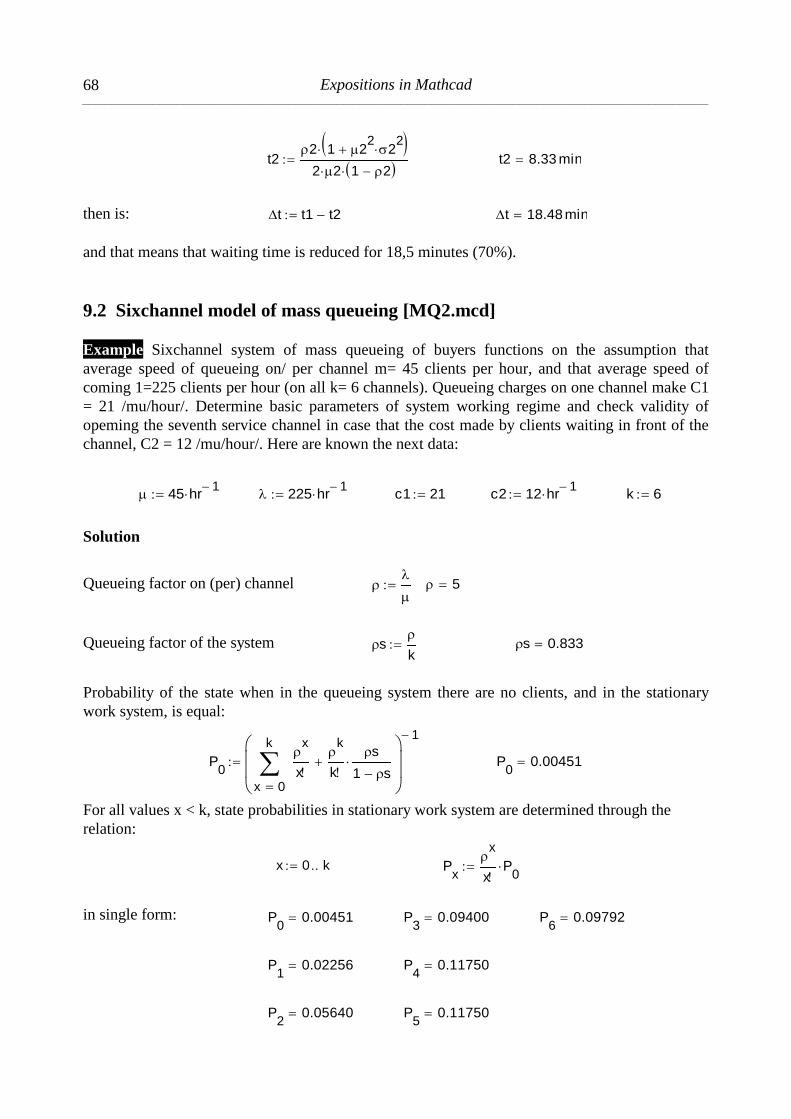
Expositions in Mathcad __________________________________________________________________________________________________________
68
t22 1 2
22
2
2 2 1 2 t2 8.33 min
then is: t t1 t2 t 18.48 min
and that means that waiting time is reduced for 18,5 minutes (70%).
9.2 Sixchannel model of mass queueing [MQ2.mcd]
Example Sixchannel system of mass queueing of buyers functions on the assumption that
average speed of queueing on/ per channel m= 45 clients per hour, and that average speed of
coming 1=225 clients per hour (on all k= 6 channels). Queueing charges on one channel make C1
= 21 /mu/hour/. Determine basic parameters of system working regime and check validity of
opeming the seventh service channel in case that the cost made by clients waiting in front of the
channel, C2 = 12 /mu/hour/. Here are known the next data:
45 hr1
225 hr1
c1 21 c2 12 hr1
k 6
Solution
Queueing factor on (per) channel
5
Queueing factor of the system s
k s 0.833
Probability of the state when in the queueing system there are no clients, and in the stationary
work system, is equal:
P0
0
k
x
x
x
k
k
s
1 s
1
P0
0.00451
For all values x < k, state probabilities in stationary work system are determined through the
relation:
x 0 k Px
x
xP
0
in single form:
P0
0.00451 P3
0.09400 P6
0.09792
P1
0.02256 P4
0.11750
P2
0.05640 P5
0.11750

Operations Research __________________________________________________________________________________________________________
69
or in vector form:
P0
P1
P2
P3
P4
P5
P6
0.00451
0.02256
0.05640
0.09400
0.11750
0.11750
0.09792
Average number of clients that waits for service:
G
6
k
s
1 s 2 P
0 G 2.94
Average total of clients that waits is queued in service channels:
Q 1 P1
2 P2
3 P3
4 P4
5 P5
6 1 P0
P1
P2
P3
P4
P5
Q 5
Average number of clients delaying in the queueing system:
Average time of clients waiting in queue
Average time of clients delayin in the system (waiting and queueing)
T 1
T 0.0353 hr T 2.12 min
Specific costs of delaying on account of clients waiting for service
Tv c2 G Tv 0.46
Then follows the statement that it is not economically to open the seventh working place for the
job of queueing clients.
10. SIMULATION MODELING
10.1 Random number generation [SM16.mcd]
In order to perform efficiently numerical modeling of random phenomena that can be described
by functions, it is necessary to possess random number generator. As basis often is used random
number uniformly disposed in standard interval [0,1]. In that case one may use Mathcad function
G
47.001 s 0.013 hr
R G Q R 7.938
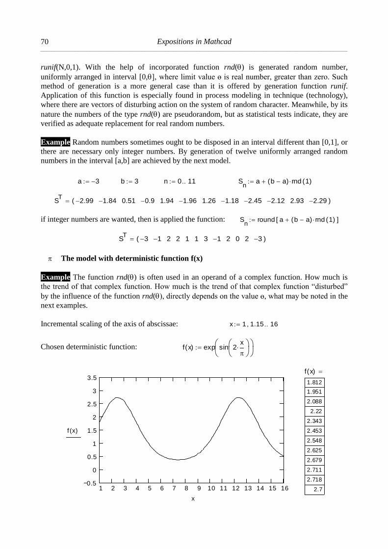
Expositions in Mathcad __________________________________________________________________________________________________________
70
runif(N,0,1). With the help of incorporated function rnd() is generated random number,
uniformly arranged in interval [0,], where limit value ө is real number, greater than zero. Such
method of generation is a more general case than it is offered by generation function runif.
Application of this function is especially found in process modeling in technique (technology),
where there are vectors of disturbing action on the system of random character. Meanwhile, by its
nature the numbers of the type rnd() are pseudorandom, but as statistical tests indicate, they are
verified as adequate replacement for real random numbers.
Example Random numbers sometimes ought to be disposed in an interval different than [0,1], or
there are necessary only integer numbers. By generation of twelve uniformly arranged random
numbers in the interval [a,b] are achieved by the next model.
a 3 b 3 n 0 11 Sn
a b a( ) rnd 1( )
ST
2.99 1.84 0.51 0.9 1.94 1.96 1.26 1.18 2.45 2.12 2.93 2.29( )
if integer numbers are wanted, then is applied the function: Sn
round a b a( ) rnd 1( )[ ]
ST
3 1 2 2 1 1 3 1 2 0 2 3( )
The model with deterministic function f(x)
Example The function rnd() is often used in an operand of a complex function. How much is
the trend of that complex function. How much is the trend of that complex function “disturbed”
by the influence of the function rnd(), directly depends on the value ө, what may be noted in the
next examples.
Incremental scaling of the axis of abscissae: x 1 1.15 16
Chosen deterministic function: f x( ) exp sin 2x
1 2 3 4 5 6 7 8 9 10 11 12 13 14 15 160.5
0
0.5
1
1.5
2
2.5
3
3.5
f x( )
x
f x( )
1.812
1.951
2.088
2.22
2.343
2.453
2.548
2.625
2.679
2.711
2.718
2.7

Operations Research __________________________________________________________________________________________________________
71
Fig. 10.1 Graph (plot)of the function with determinated trend
Model of the function f(x) with weaker trend disturbance
The function f(x) with added operand rnd(): f x( ) exp sin 2x
rnd 0.3( )
1 2 3 4 5 6 7 8 9 10 11 12 13 14 15 160.5
0
0.5
1
1.5
2
2.5
3
3.5
f x( )
x
f x( )
1.96
2.173
2.274
2.461
2.516
2.727
2.767
2.825
2.774
2.802
2.75
2.955
Fig. 10.3 Graph (plot) of the function with random trend-variable with weaker trend
Model of the function f(x) with marked trend disturbance
The function f(x) with added operand rnd(): f x( ) exp sin 2x
rnd 1.4( )
1 2 3 4 5 6 7 8 9 10 11 12 13 14 15 160
0.5
1
1.5
2
2.5
3
3.5
4
4.5
f x( )
x
f x( )
2.668
3.177
2.921
3.33
3.17
3.25
3.49
2.639
3.157
3.79
3.935
3.716

Expositions in Mathcad __________________________________________________________________________________________________________
72
Fig. 10.4 Graph (plot) of the function with random trend-variable with more marked disturbed
trend
Advice In order to make the procedures for random numbers more authentic, it is necessary to
change periodically the value of “seed” of random numbers generator. This change is done by the
option seed value for random numbers in the menu Math Options… Value “seed” is initial
value of the numerical algorithm rnd and is defined that it is always equal or greater than one.
10.2 Simulating time reliability of technical system elements [SM2_a.mcd]
Example The elements of the technical system S1, S2 and S3 are connected series-parallel
according to the fig.1. On the basis of N= 4000 simulations, calculate mean time of system work
without failure and compare it with theoretical result, if for every element, times of work without
failure are exponentially disposed with known intensities of failure and 3. Calculate
relative aberration of theoretical and simulated mean value of time failure. Graphically present the
functions of single and superponerated reliability.
S1
S3
S2
Fig. 10.5 The chart of the system S of technical elements in parallel connection
Symbolical value solution of system reliability at series-parallel connection of
elements
Functions of exponential reliability for three elements apart:
R1 1 t e1 t
R2 2 t e2 t
R3 3 t e3 t
Total superponerated reliability function:
R 1 2 3 t e1 t
1 1 e2 t
1 e3 t
Symbolical solution for mean failure time of system at this combined connection of elements S1,
S2 and S3:

Operations Research __________________________________________________________________________________________________________
73
0
tR 1 2 3 t
d
assume 1 0
assume 2 0
assume 3 0
12
2 1 2 2 1 3 22
2 3 32
1 3 1 2 1 2 3
Theoretical value of system reliability at parallel connection of elements
Failure intensities of single elements make:
S1: 1 0.35 103
S2: 2 0.28 103
S3: 3 0.32 103
Total theoretical reliability for parallel connection:
R t( ) R1 1 t 1 1 R2 2 t 1 R3 3 t
Theoretical mean time of system reliability at parallel connection of elements S1, S2 and S3:
Trp
0
tR t( )
d or concretely: Trp 2027.2073217870547014
Mean time of elements reliability 1:
0
te1 t
d 2857.1428571428571429
Mean time of elements reliability 2:
0
te2 t
d 3571.4285714285714286
Mean time of elements reliability 3:
0
te3 t
d 3125.0000000000000000
Mean time of elements reliability at series connection of elements S1, S2 and S3:
Simulation of system reliability at parallel connection of elements
Simulation of reliability time for S1:
Number of simulations: N 4000 i 0 N 1
T1 rexp N 1 T1T 0 1 2 3 4 5
0 173.5 3024.5 908.3 74.5 2 3350
Mean time of failure of elements for S1: mean T1( ) 2874.488
Simulation of reliability time for S2:
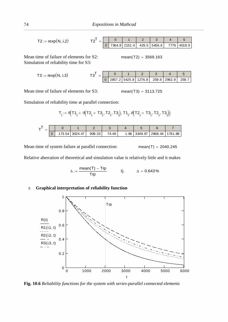
Expositions in Mathcad __________________________________________________________________________________________________________
74
T2 rexp N 2 T2T 0 1 2 3 4 5
0 7364.8 2151.4 429.5 5456.6 7776 4018.9
Mean time of failure of elements for S2: mean T2( ) 3569.163 Simulation of reliability time for S3:
T3 rexp N 3 T3T 0 1 2 3 4 5
0 2857.2 5425.8 1276.8 259.8 2962.9 259.7
Mean time of failure of elements for S3: mean T3( ) 3113.725
Simulation of reliability time at parallel connection:
T
iif T1
iif T2
iT3
i T2
i T3
i T1
i if T2
iT3
i T2
i T3
i
TT 0 1 2 3 4 5 6 7
0 173.54 3024.47 908.33 74.49 1.96 3349.97 2968.44 1761.88
Mean time of system failure at parallel connection: mean T( ) 2040.245
Relative aberration of theoretical and simulation value is relatively little and it makes
mean T( ) Trp
Trp tj. 0.643 %
Graphical interpretation of reliability function
0 1000 2000 3000 4000 5000 60000
0.2
0.4
0.6
0.8
1
R t( )
R1 1 t( )
R2 2 t( )
R3 3 t( )
Trp
t
Fig. 10.6 Reliability functions for the system with series-parallel connected elements

Operations Research __________________________________________________________________________________________________________
75
As the number of replication increases, we note convergence of simulation result to very precise
(one). This way of evaluation is enabled, because the results of referenced model are known, i.e.
analytical one. In simpler cases of reliability modeling may be formed both models, then compare
their results. In more complex cases, it is often is only possible to apply Monte Carlo method, so
because of that reason it is called “method of the last output (solution)” [29].
11. MATRIX GAMES
11.1 Nonsingular matrix games [MG1.mcd]
Example Some two players may choose one of the next three numbers 0, 1 and 2. If addition of
three numbers is even, then it goes to the second player, and if it is odd, to the first (one).
Payment matrix for this game is:
A
0
1
2
1
2
3
2
3
4
This matrix is singular, so here can not directly be applied the method of calculation for defining
optimal mixed strategies. Meanwhile, if to every element of this matrix is added one, we shall get
the matrix C.
B
1
1
1
1
1
1
1
1
1
C A B
1
2
1
2
1
4
1
4
3
Inverse matrix of C matrix is equal: C1
13
16
1
8
7
16
1
8
1
4
3
8
7
16
3
8
5
16
so the value of this modified game is: V1
IT
C1
I
1
where is: I
1
1
1
because: IT
C1
I 1( ) in other words the value of starting game is equal to 0. optimal mixed
strategies both for starting and modified game, are:

Expositions in Mathcad __________________________________________________________________________________________________________
76
pIT
C1
IT
C1
I
1
4
1
2
1
4
and qC
1I
IT
C1
I
1
4
1
2
1
4
12. INVENTORY CONTROL
12.1 The calculation of optimal quantities of inventory with constant
procurement [IC1.mcd]
Example A trade company plans to acquire Q= 1600 /pieces/ (of) products during period τ= 1
/year/ (365 days). The buying price of the order is K0 = 83 /mu/, while annual charges for storage
k1 = 5,6 /mu/kom/. Calculate:
a) Optimal quantity qo that ought to be contained in order so that total costs of inventories
would be minimized.
b) Calculate adequate quantity of products by order q1 and q2 /pieces/, if total charges of
inventories increase for p= 50%. Realize comparison in relation to optimal quantity of
products.
c) Give graphical presentation of flows for stockpiling and spending of product inventories for
found numerical solutions.
Starting data
Annual quantity of products /pieces/: Q 1600 Plan period /years/: 1 Fixed costs of inventories ordering per series /mu/: k0 83 Costs of inventories storage /mu/pieces/year/: k1 5.6 Percentage of increased costs for intervened storage in relation to regular one: p 50 %
Solution
Optimal quantity of ordering /pieces/: qo2 Q k0
k1 qo 217.78
Optimal number of annual series /ser/years/: nQ
qo n 7.35
Time period of one series /year/: t
n t 0.136
Minimal expenses of inventory /mu/: F k0Q
qo k1
qo
2 F 1219.57

Operations Research __________________________________________________________________________________________________________
77
or: minF 2 k0 k1 Q minF 1219.57
Expenses increased for p.percentage /mu/: F1 1 p( ) F F1 1829.36
Equation of total expenses: k0Q
q k1
q
2 F1 0
that is equivalent to square equation:
k1
2 q
2 F1 q k0 Q 0
Solving root of equation on the basis of equation coefficients: q12
k0 Q
F1
k1
2
ORIGIN 1 q1
q2
polyroots q12( )
Two solutions of square equation make /pieces/:
q1
q2
83.185
570.158
Alternative marks: q1 q1
q2 q2
Relation of two inventory quantities: uq2
q1 u 6.854
Graphical interpretation of increased inventory costs for p= 50%.
Axis scaling of inventory quantity: q 0 1 650
Function of total costs: f q( ) k1q
2 k0
Q
q

Expositions in Mathcad __________________________________________________________________________________________________________
78
0 100 200 300 400 500 6000
1000
2000
3000
F
F1f q( )
k0Q
q
k1q
2
q1 q2
q
Fig. 12.1 Functions of total and partial costs
Scaling of independent variable: x 0t
200 ceil n( ) t
Inventory programming in time for the first nine series:
f x( ) qo 1
x
t
0 x tif
qo 2x
t
t x 2 tif
qo 3x
t
2 t x 3 tif
qo 4x
t
3 t x 4 tif
qo 5x
t
4 t x 5 tif
qo 6x
t
5 t x 6 tif
qo 7x
t
6 t x 7 tif
qo 8x
t
7 t x 8 tif
In view of previous data we can plan inventory quantities for operative period, during so-called
“sowlike” diagram.

Operations Research __________________________________________________________________________________________________________
79
0 0.2 0.4 0.6 0.8 10
100
200
qo
f x( )
x
Sl. 12.2 Dijagram stanja zaliha u vremenu
12.2 Calculation of optimal inventory quantities with intervened order
[IC2.mcd]
Example In the case that demand for inventory is greater than regularly acquired quantity,
calculate.
a) Optimal volume q of demand on inventories during time period t as well optimal volume of
inventories p in the same time interval t. Because of that calculate intervened quantity ∆ q.
b) Optimize interval cycle t(time between previous and next series), as well number of orders
during time τ = 12 /months (365 days), if the next data are given:
Q = 245000 / pieces/ - total demand during year, k1= 80 /mu/pieces/months / - unit costs of
inventory maintenance, k2= 260/nj/pieces/months/ - costs that appear an account of uneven
delivering of inventory, k0 = 7300 /mu/- fixed costs of series acquisition.
c) Determine necessary quantity p and ∆q, if new quantity q = 3400 /pieces/, and total costs of
inventory in new conditions make F=11900000 /mu/. The other parameters remain the some
as under b).
d) Present graphically the case under c).
Starting data
Annual quantity of products /pieces/: Q 245000 Planned period of inventory converting /months/: 12 Fixed costs of inventory per series /mu/: k0 7300 Costs of inventory storage /mu/pieces/months/: k1 80 Costs of storage of intervened quantity of inventory /mu/pieces/months/: k2 260
Solution
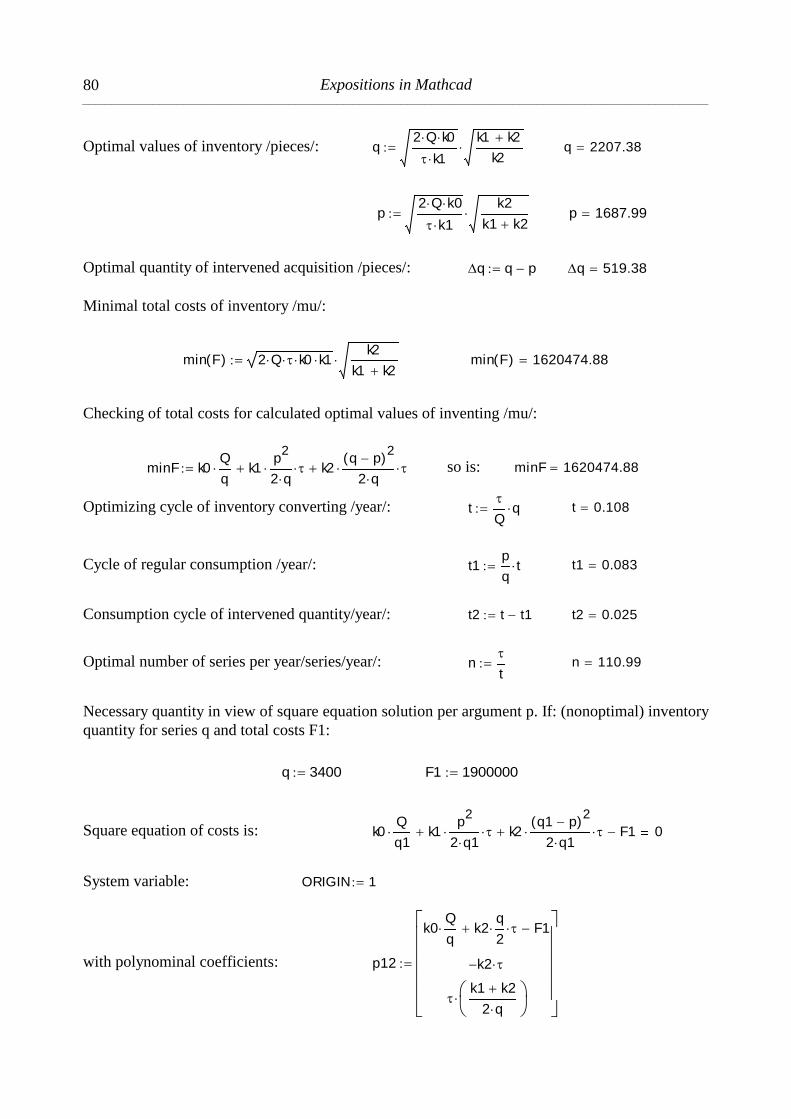
Expositions in Mathcad __________________________________________________________________________________________________________
80
Optimal values of inventory /pieces/: q2 Q k0
k1
k1 k2
k2 q 2207.38
p2 Q k0
k1
k2
k1 k2 p 1687.99
Optimal quantity of intervened acquisition /pieces/: q q p q 519.38
Minimal total costs of inventory /mu/:
min F( ) 2 Q k0 k1k2
k1 k2 min F( ) 1620474.88
Checking of total costs for calculated optimal values of inventing /mu/:
minF k0Q
q k1
p2
2 q k2
q p( )2
2 q so is: minF 1620474.88
Optimizing cycle of inventory converting /year/: t
Qq t 0.108
Cycle of regular consumption /year/: t1p
qt t1 0.083
Consumption cycle of intervened quantity/year/: t2 t t1 t2 0.025
Optimal number of series per year/series/year/: n
t n 110.99
Necessary quantity in view of square equation solution per argument p. If: (nonoptimal) inventory
quantity for series q and total costs F1:
q 3400 F1 1900000
Square equation of costs is:
k0Q
q1 k1
p2
2 q1 k2
q1 p( )2
2 q1 F1 0
System variable:
with polynominal coefficients: p12
k0Q
q k2
q
2 F1
k2
k1 k2
2 q
ORIGIN 1

Operations Research __________________________________________________________________________________________________________
81
Possible order p /pieces/ makes: p1
p2
polyroots p12( )
p1
p2
2141.8
3058.2
It follows that intervened quantity /pieces/in these conditions equal:
q1 q p1 q1 1258.204 q2 q p2 q2 341.796
cycle of regular consumption /years/: t11p1
qt t11 0.068
Consumption cycle of intervened quantity /year/:
t21 t t11 t21 0.04 t12p2
qt t12 0.097 t22 t t12 t22 0.011
Verification of costs solution /um/:
k0Q
q k1
p12
2 q k2
q p1( )2
2 q
k0Q
q k1
p22
2 q k2
q p2( )2
2 q
1900000
1900000
and it full suits to previously defined costs:
13. NETWORK PLANNING
13.1 Application of network technique PERT [PN1.mcd]
Example Determine expected values of time and standard deviation for set of six activities, given
through network diagram (fig.13.1). Optimistic (a), the most probable (m) and pessimistic (b)
times are presented in vector way. Check probability P of critical path realization in PERT
network if the planned time of its realization Tp = 12 days.
t0
1
2
4
3
5
s0
t2
s2
t3
s3
t5
s5
t4
s4
t1
s1
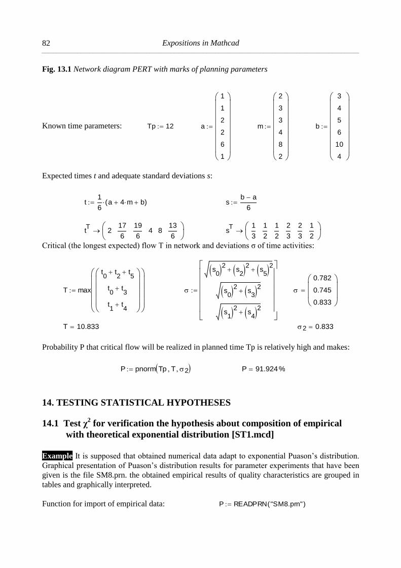
Expositions in Mathcad __________________________________________________________________________________________________________
82
Fig. 13.1 Network diagram PERT with marks of planning parameters
Known time parameters: Tp 12 a
1
1
2
2
6
1
m
2
3
3
4
8
2
b
3
4
5
6
10
4
Expected times t and adequate standard deviations s:
t1
6a 4 m b( ) s
b a
6
tT
217
6
19
64 8
13
6
sT 1
3
1
2
1
2
2
3
2
3
1
2
Critical (the longest expected) flow T in network and deviations σ of time activities:
T max
t0
t2
t5
t0
t3
t1
t4
s0 2 s
2 2 s5 2
s0 2 s
3 2
s1 2 s
4 2
0.782
0.745
0.833
T 10.833 2 0.833
Probability P that critical flow will be realized in planned time Tp is relatively high and makes:
P pnorm Tp T 2 P 91.924%
14. TESTING STATISTICAL HYPOTHESES
14.1 Test χ2 for verification the hypothesis about composition of empirical
with theoretical exponential distribution [ST1.mcd]
Example It is supposed that obtained numerical data adapt to exponential Puason’s distribution.
Graphical presentation of Puason’s distribution results for parameter experiments that have been
given is the file SM8.prn. the obtained empirical results of quality characteristics are grouped in
tables and graphically interpreted.
Function for import of empirical data: P READPRN "SM8.prn"( )
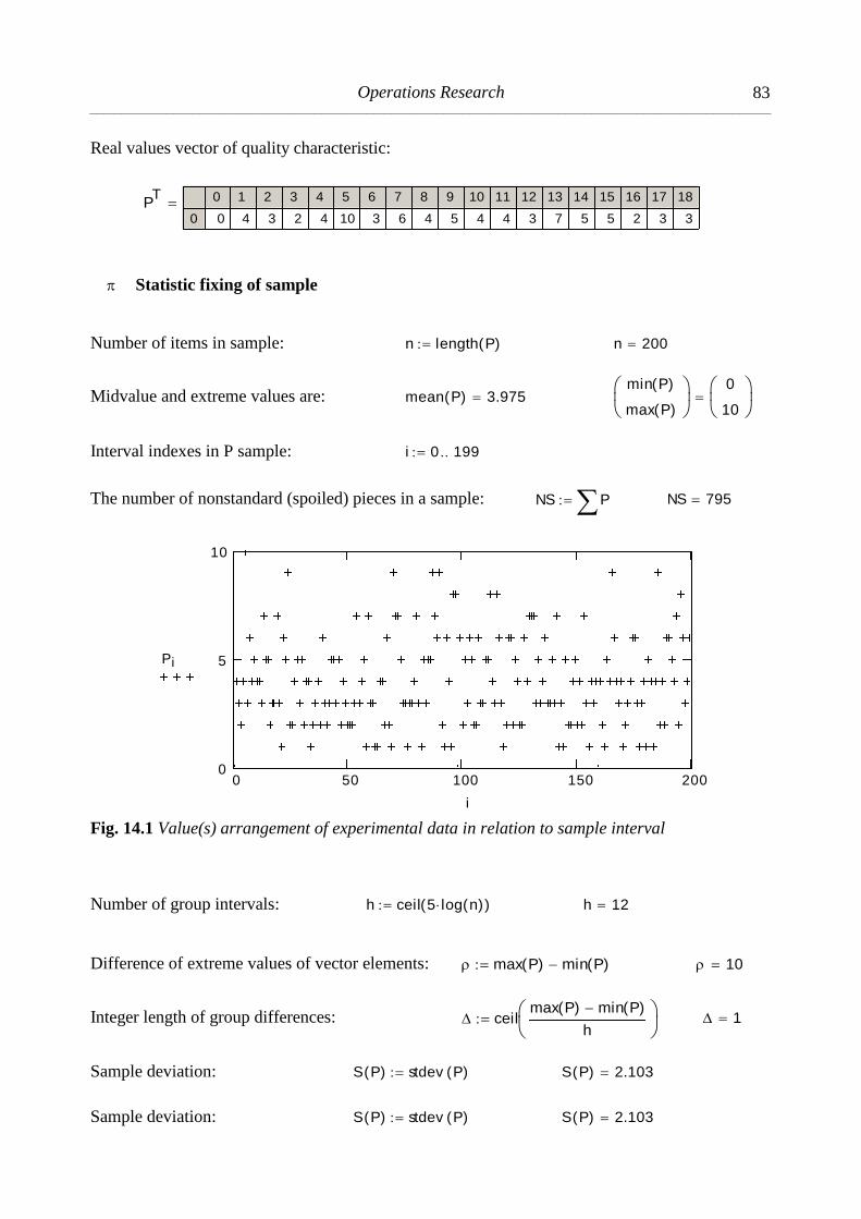
Operations Research __________________________________________________________________________________________________________
83
Real values vector of quality characteristic:
PT 0 1 2 3 4 5 6 7 8 9 10 11 12 13 14 15 16 17 18
0 0 4 3 2 4 10 3 6 4 5 4 4 3 7 5 5 2 3 3
Statistic fixing of sample
Number of items in sample: n length P( ) n 200
Midvalue and extreme values are: mean P( ) 3.975 min P( )
max P( )
0
10
Interval indexes in P sample: i 0 199
The number of nonstandard (spoiled) pieces in a sample: NS P NS 795
0 50 100 150 2000
5
10
Pi
i
Fig. 14.1 Value(s) arrangement of experimental data in relation to sample interval
Number of group intervals: h ceil 5 log n( )( ) h 12
Difference of extreme values of vector elements: max P( ) min P( ) 10
Integer length of group differences: ceilmax P( ) min P( )
h
1
Sample deviation: S P( ) stdev P( ) S P( ) 2.103 Sample deviation: S P( ) stdev P( ) S P( ) 2.103

Expositions in Mathcad __________________________________________________________________________________________________________
84
Marginal values of intervals of fixed set of data: j 0 h
Marginal values vector of group intervals: I
jmin P( ) j
IT 0 1 2 3 4 5 6 7 8 9 10 11 12
0 0 1 2 3 4 5 6 7 8 9 10 11 12
Function of histograms in vector form: f hist I P( )
fT 0 1 2 3 4 5 6 7 8 9 10 11
0 3 19 31 40 34 26 21 14 5 6 1 0
Funkcija fitovane normalne raspodele: ft x( ) n dpois x mean P( )( ) Frequency of fitted data in h (of ) group intervals: k 0 h 1 Frequencies: empirical, theoretical sum of frequencies:
fk
3
19
31
40
34
26
21
ft Ik 3.756
14.93
29.672
39.316
39.07
31.061
20.578
f 200
k
ft Ik 199.83
Graphical interpretation of sample date distribution
1 0 1 2 3 4 5 6 7 8 9 10 11 120
5
10
15
20
25
30
35
40
45
histogram
poligon poligon
fk
fk
ft Ik
min P( ) max P( ) 1
Ik

Operations Research __________________________________________________________________________________________________________
85
Fig. 14.2 Histogram and polygon of empirical and polygon of theoretical distribution
Difference function of empirical and theoretical values of distribution: k f
kft I
k
1 1 3 5 7 9 11 1310
7.5
5
2.5
0
2.5
5
7.5
10
"stem"
0k
min P( ) max P( ) 1
Ik
Ik
0
1
2
3
4
5
6
7
8
9
10
11
k
-0.756
4.07
1.328
0.684
-5.07
-5.061
0.422
2.315
-0.806
3.436
-0.019
-0.368
Fig. 14.3 “Stem” form of aberration function
Note In the next procedure has been performed grouping of starting and final values of
frequencies, so that the value of these additions, as new elements frequencies vectors would not
be lesser (fewer) than 5. In this case (it) is reduced with 12 on 9 elements given in the next tables
(following).
Distribution correction of empirical and theoretical frequencies in (m+1) interval(s):
m h 1( ) 4 m 8 g 0 m
Fg
f0
f1
f2
f3
f4
f5
f6
f7
f8
f9
f10
f11
Ftg
ft I0 ft I
1
ft I2
ft I3
ft I4
ft I5
ft I6
ft I7
ft I8
ft I9 ft I
10 ft I11
Fg
22
31
40
34
26
21
14
5
7
Ftg
18.685
29.672
39.316
39.07
31.061
20.578
11.685
5.806
3.952
Fg
Ftg
3.315
1.328
0.684
-5.07
-5.061
0.422
2.315
-0.806
3.048
Fg
Ftg
2
10.987
1.762
0.468
25.708
25.613
0.178
5.358
0.65
9.29
g
0
1
2
3
4
5
6
7
8
Hypothesis testing about presumed distribution

Expositions in Mathcad __________________________________________________________________________________________________________
86
Testing is performed on the basis of hi-square test:
Empirical value of hi-square makes: 2
g
Fg
Ftg
2
Ftg
2 5.072
Risk and certainty of hypothesis acceptance of (about) accordance of empirical and theoretical
distribution:
0.10 1 90%
Number of unknown parameters of basic population (value ): s 1
Number of addends in the expression for hi-square value: r m 1 r 9 Number of freedom degree: r s 1
Theoretical (limited) value hi-square: 2g qchisq 1 2g 12.017
Axis scaling of hi-square frequency: q 0 0.1 25 k 0 1
0 5 10 15 20 250
0.03
0.06
0.09
0.12
0.150.15
0
dchisq q ( )
0
dchisq 2 g
k
250
2 2 g
q 2 g
Fig. 14.4 Graphical presentation of hypothesis testing on the basis of distribution hi-square
Results of testing with Hi-square test
Hi-square testing results may be quantatively expressed by confirming or rejecting the next
hypotheses:
Operations Research __________________________________________________________________________________________________________
87
- Hypothesis H0: Empirical data are submitted to the theoretical low of exponential
distribution.
- Hypothesis H1: Deviation empirical from theoretical distribution has no random character.
Control vector of hi-square value: 0 2 2g 0 5.072 12.017( )
Allowed hi-square values: 0 2 2g 1
Area of accepting H0 hypothesis: pchisq 2 1 1
If: a) result is 1 we accept H0 hypothesis
b) result is 0 we accept H1 hypothesis.
Conclusion On the basis of confirming H0 hypothesis, we can with high probability of 90%
claim that general population, from which the sample is analyzed, corresponds with supposed
Puason’s distribution low. Thus, hypothesis about this distribution does not contradict to
empirical data.
14.2 Testing hypothesis about samples homogenity in view of their
variances [ST2.mcd]
Example Perform statistical F-hypothesis testing about marks equality in the mathematics subject
with two pupils population on the basis of variances marks. Basic function of variances analysis
is to find out are there statistically significant deviations between selected sharacteristics of two
groups of among many groups in population. In pedagogical sense it e.g. can be marks of pupils
knowledge, time periods of education in certain areas and the like. Thereby, values, that in
principle, may be qantified. If it is found that that difference between characteristics of some
groups statistically significant, then it is the proof that they do not belong to the same population,
and that pedagogical concluding on their baisis is unreliable. If it is found that that difference
statistically insignificant (little or that is does not exist), then it is proof that there are groups, e.g.
pupils, that belong to the same population and that pedagogical concluding on their basis reliable.
Calculations of vareinces and all other procedures that follow are basically simple, if user has
certain foreknowledge, so that he could explain inter and final results. They are established
through shecked statistical procedures. Here, these procedures will be illustrated on the results of
application Fisher's F-test, by which we can find (non) equalities of marks at one subject. In this
case is chosen mathematics and the example is made on the basis of methodology elaborated in
the reference [27]. Testing of differences significances among statistical values is performed
comparing value pairs from two series of statistical date, through analysis of variances.
Significance of differences between two groups of pupils of the same generation in Mathematics
subject. Set of marks for every group has been formed in separate files: group1.prn and
group2.prn. Through Mathcad they are taken over as numerical data, forming vectors of S1 and
S2 marks, through an adress with articulated path. Number of pupils is not the same for every
group, and for every pupil is recorded only one mark. On account of more efficient an more
suitable application, separately will be interpreted and illustrated tabling of data (vector of
numbers, i.e. marks) and later graphically presented F-test results.

Expositions in Mathcad __________________________________________________________________________________________________________
88
of the first group: S1 READPRN "gr1.prn"( )
of the second grpoup: S2 READPRN "gr2.prn"( )
S1T 0 1 2 3 4 5 6 7 8 9 10 11 12 13 14 15 16 17 18 19 20
0 5 4 2 3 4 5 4 4 3 4 3 5 3 4 2 5 4 3 5 5 4
S2T 0 1 2 3 4 5 6 7 8 9 10 11 12 13 14 15 16 17 18 19 20
0 4 3 1 4 5 4 5 3 4 2 4 5 3 5 5 4 4 5 2 5 4
Number of tested pupils of the first group: n1 length S1( ) n1 59
Number of tested pupils of the second group: n2 length S2( ) n2 45
Accepted probability of mistake of hypothesis accepting about homogenity of marks:
0.10 10%
Accepted probability of hypothesis accepting about homogenity of marks:
1 0.9 1 90%
Standard deviation and variance of samples:
prve grupe: stdev S1( ) 0.9579 var S1( ) 0.918
druge grupe: stdev S2( ) 1.0376 var S2( ) 1.077
Objective mark of samples variance:
of the first group: v1n1
n1 1var S1( ) v1 0.9334
of the second group: v2n2
n2 1var S2( ) v2 1.101
Minimal, average and i maximal mark of samples:
of the first group: min S1( ) 2 mean S1( ) 3.78 max S1( ) 5
of the second group: min S2( ) 1 mean S2( ) 3.889 max S2( ) 5
F–hypothesis testing of pupils' marks equality

Operations Research __________________________________________________________________________________________________________
89
Number of freedom degrees:
of the first group: 1 n1 1 1 58
of the second group: 2 n2 1 2 44
Upper threshold of significance: F1 qF
21 2
F1 0.6308
Lower threshold of significance: F2 qF 1
2 1 2
F2 1.6134
Variable of F distribution: F ifv1
v21
v1
v2
v2
v1
F 1.1796
Note The variable F is necessary to nominate to be greater than 1. In that sense if function is
used.
Scaled values of independent variable: q 0 0.02 4 k 0 1
0 0.6 1.2 1.8 2.4 30
0.32
0.64
0.96
1.28
1.6
dF q 1 2( )
0
dF F1 1 2( )
k
0
dF F2 1 2( )
k
F
q F1 F2
Fig. 14.5 Graphical presentation of hypothesis testing on the basis of F-distribution
Control vector of limit F values: F1 F F2( ) 0.6308 1.1796 1.6134( )
Hypothesis H0: 012
022 that variances of basic sets are nutually equal.

Expositions in Mathcad __________________________________________________________________________________________________________
90
Hypothesis H1: 012
022
that among variances of basic sets (there) are significant
differences.
Interval of confidence:
2pF F 1 2 1
2 1
Area of H0 hypothesis accepting: F1 F F2 1
Test criterion: If: a) result is 1 H0 hypothesis is accepted
b) result is 0 H1 hypothesis is accepted.
Conclusion Hypothesis H0 is confirmed. In that case it can be stated that estimates of variances
are not significantly differetn, so there are no bases for suppostition that one group of pupils has
achieved better results in mathematics than the other one. Here presented method of pedagogical
research may be base for development of extended model of pedagogical experiment on the basis
of new and more detailed data.
Reference
[1] Backović, M. i Vuleta, J. EKONOMSKO MATEMATIČKI METODI I MODELI,
Ekonomski fakultet, Beograd, 2004.
[2] Backović, M., Vuleta, J., Prica, I. i Popović, Z. EKONOMSKO MATEMATIČKI METODI
I MODELI, Zbirka rešenih problema, Ekonomski fakultet, Beograd, 2004.
[3] Baets, B., Fodor, J. i Radojević, D. (Editors). FUZZY FOR BETTER, Eurofuse
Anniversary Workshop, Institut “Mihajlo Pupin”, Belgrade, 2005.
[4] Burton, V. D. OPERACIONA ISTRAŽIVANJA U ISTRAŽIVANJIMA I RAZVOJU,
(prevod Zbornika radova), “Savremena administracija”, Beograd, 1968.
[5] Cvetković, D., Kovačević-Vujčić, V. (redaktori) KOMBINATORNA OPTIMIZACIJA,
Matematička teorija i algoritmi, “DOPIS”, Beograd, 1996.
[6] Ćerić, V. METODE VREDNOVANJA SIMULACIONIH MODELA, SYM-OP-IS ‘84.,
(str. 169-177), Herceg Novi, 1984.
[7] Čileg, M., Vugdelija, D. i Kiš, T. OPERACIONA ISTRAŽIVANJA, Zbirka zadataka sa
rešenjima, Ekonomski fakultet, Subotica, 1996.
[8] Čupić, M., Suknović, M., Radojević, G. i Jovanović, V. SPECIJALNA POGLAVLJA IZ
TEORIJA ODLUČIVANJA: KVANTITATIVNA ANALIZA, Univerzitet u Novom Sadu,
Fakultet tehničkih nauka, Novi Sad, 2004.
[9] Dantzig, G, B. LINEAR PROGRAMMING AND EXTENSIONS, Princeton University
Press, Princeton, New Jersey, 1963.
[10] Fishman, S. G. MONTE CARLO CONCEPTS, ALGORITHMS AND APPLICATIONS,
Springer Series in Operations Research, Springer, 1999.
[11] Ivanović, G. i Stanivuković, D. POUZDANOST TEHNIČKIH SISTEMA - Zbirka rešenih
zadataka, Univerzitet u Beogradu, Mašinski fakultet, Beograd, 1987.
[12] Krčevinac, S., Čangalović, M., Kovačević-Vujić, V., Martić, M. i Vujošević, M.
OPERACIONA ISTRAŽIVANJA, Fakultet organizacionih nauka, Beograd, 2004.

Operations Research __________________________________________________________________________________________________________
91
[13] Kun, L. PRIMENA ISTRAŽIVANJA OPERACIJA, Mašinski fakultet, Novi Sad, 1973.
[14] Letić, D., Davidović, B., Berković, I. i Petrov, T. MATHCAD 13 U MATEMATICI I
VIZUELIZACIJI, Kompjuter biblioteka, Čačak, 2007.
[15] Letić, D.i Jevtić, V. OPERACIONA ISTRAŽIVANJA, Tehnički fakultet “M. Pupin”,
Zrenjanin, 2006.
[16] Marinković, M. OPERACIONA ISTRAŽIVANJA, Viša škola za organizaciju rada,
Novi Sad, 1987.
[17] Nikolić, VIŠEKRITERIJUMSKA OPTIMIZACIJA – METODE, LOGISTIKA, SOFTVER,
Visoka vojna škola Vojske Jugoslavije, Beograd, 1999.
[18] Opricović, S. OPTIMIZACIJA SISTEMA – ZADACI IZ VODOPRIVREDE I
HIDROTEHNIKE, Građevinski fakultet, Beograd, 1995.
[19] Petrić, J. OPERACIONA ISTRAŽIVANJA I i II, Naučna knjiga, Beograd, 1989.
[20] Petrić, J., Šarenac, L. i Kojić, Z. OPERACIONA ISTRAŽIVANJA I i II, Zbirke rešenih
zadataka, Naučna knjiga, Beograd, 1992.
[21] Саздановић, С. ЛИНЕАРНО ПРОГРАМИРАЊЕ, Научна књига, Београд, 1988.
[22] Stanojević, R. METODA SIMPLEKS, ZBIRKA REŠENIH PRIMERA, Institut “Braća
Karić”, Beograd, 1996.
[23] Stojanović, D. EKONOMSKO MATEMATIČKI METODI I MODELI, Ekonomski
fakultet, Beograd, 1990.
[24] Vujanović, N. TEORIJA POUZDANOSTI TEHNIČKIH SISTEMA, Vojnoizdavački i
novinski centar, Beograd, 1987.
[25] Vujošević, M. OPERACIONA ISTRAŽIVANJA, Izabrana poglavlja, Fakultet
organizacionih nauka, Beograd, 1999.
[26] Vukadinović, S. MASOVNO OPSLUŽIVANJE, Naučna knjiga, Beograd, 1986.
[27] Vukadinović, S. ELEMENTI TEORIJE VEROVATNOĆE I MATEMATIČKE
STATISTIKE, Privredni pregled, Beograd, 1981.
[28] Вукадиновић, С. Цвејић, С. МАТЕМАТИЧКО ПРОГРАМИРАЊЕ, Универзитет у
Приштини, Приштина, 1996.
[29] Vukadinović, S. i Popović, J. METODE MONTE KARLO, Saobraćajni fakultet, Beograd,
1992.
[30] Vukičević, R. M. OPERACIONA ISTRAŽIVANJA u preradi drveta, Univerzitet u Novom
Sadu, Šumarski fakultet, Beograd, 1997.
[31] Winston, L.W. OPERATIONS RESEARCH, Applications and Algorithms, Indiana
University, Duxbury Press, Belmont, California, 1994.
[32] Zelenović, D., Ćosić, I. i Maksimović, R. PROJEKTOVANJE PROIZVODNIH SISTEMA,
Priručnik za vežbe, Nauka, Beograd, 1992.
[33] Zlobec, S., Petrić, J. NELINEARNO PROGRAMIRANJE, Naučna knjiga, Beograd, 1989.
Index
A AAP (Anti Aircraft
Protection), 9
Assignments problem, 31
B Belman, 2
Borel, E., 1
ceil(x), 76, 81
C Charens, 1
Charnes, 1
Clifford, 52
Constraints vector, 32
Expositions in Mathcad __________________________________________________________________________________________________________
90
Constraints vector, 4, 8, 15
Costs vector, 15
Criterion function, 2, 6, 7, 8,
9, 15, 36
Cuper, 1
D Danzig, G, 1
Derki-Vijbah, 59
Deterministic function, 68
dpois(x), 81
Dual criterion function, 14
Dual model LP, 13
During, 2
Dynamic programming, 2, 53
E Empirical value, 83
Erlang, A. K., 1
exp(x), 68
Extreme values, 80
F Falkerson, 1
Fazar, 2
Fisher's F-test, 85
Ford, 1
FRAME, 8
Freedom degree, 79
Function of total costs, 75
Fuzzy linear programming,
15
Fuzzy sets, 2
G Gant, H., 1
Genetic algorithms, 2
Given, 3, 7, 9, 14, 13, 21, 39,
42, 52
H Harris, 1
Heuristic research, 2, 58
Hinchin, 1
Hi-square frequency, 84
Hi-square test, 84
hist(x), 81
Hitchcock, 1
I Index values, 29
Initial value, 7
Inventory control, 73
Inventory quantity, 75, 78
K Kelly, 1
Kendal, 1
Kun, 1
L Last variable, 8
Lee, 1
Lemke, 1
length(x), 80, 85
Limit functions, 53
Linear constraints system, 14
Linear constraints, 8
Linear equations system, 16
Linear programming, 2, 4, 7,
10
Logical solution, 7
Logical verification, 12
M Marginal values, 81
Markov matrix, 61, 63
Markov models, 61
Mass queueing, 65, 66
Mathematical model, 53
max(x), 56, 58, 80
maximize(x), 3, 7, 8, 14, 16,
17, 34, 53
Maximum profit, 17
Maximum value, 15
mean(x), 70, 72, 80
Metropolis, 1
min(x), 77, 80
Minimal expenses, 17, 24,
25, 28
Minimal total costs, 77
Minimal value, 14
minimize(x), 12, 14, 16, 18,
27, 34, 47
Monte-Carlo method, 1, 72
Morgenstern, 1
Multicriteria optimization,
57
Multicriteria programming,
2
N Network planning, 79
Neumann, Von, 1
Neuron networks, 2
Non-equation system, 10
Nonlinear programming, 2,
44, 46
Number of columns, 28
Number of rows, 28
O One-dimensional process,
53
Optimal plan, 37
Optimal resources
distribution, 53
Optimal solutions, 18
Optimal transport plan, 21,
32
Optimization, 4, 9
ORIGIN, 8, 12, 17, 22, 24,
31, 32, 38, 41
P pchisq(a,b), 84
PDM (Precedence
Diagramming Method), 2
PERT, 1, 79
pnorm(x), 80
Polachek, 1
Polynominal coefficients,
78
polyroot(x), 75, 78
Production program, 12, 16
Profit function, 15, 20, 24
Profit maximum, 21
Puason’s distribution, 80
Q qchisq(x), 83
Queueing factor, 66

Operations Research __________________________________________________________________________________________________________
91
R Random number generation,
67
READPRN(x.prn), 80, 85
rnd(x), 68, 69
round(x), 68
S Sample deviation, 79
Simulation modeling, 67
Simulation of reliability time,
71, 72
Solution verification, 17, 28
Solution verification, 8
stack(x,y), 16, 18, 30, 62
Statistical hypotheses, 80
stdev(x), 81, 85
submatrix(x), 64, 65
Sum of capacities, 29
Supplementary variables, 17
System variable, 6
T Taylor, Frederick, 1
Transportation problem, 15,
19, 26
Tucker,1
U Ulman,1
V Valker, 1
var(x), 85, 86
Vogel, 1
Z Zadeh, 2