operations research models for railway rolling stock planning
TRANSCRIPT

Operations Research Models for
Railway Rolling Stock Planning
Gabor Maroti

Maroti, Gabor
Operations research models for railway rolling stock planning / Gabor Maroti. –
Eindhoven, Technische Universiteit Eindhoven, 2006.
Proefschrift. – ISBN 90-386-0744-X. – ISBN 978-90-386-0744-3
NUR 919
Subject headings: railway transportation / integer programming / network optimisation
2000 Mathematics Subject Classification: 90B06, 90C35, 90C11
Operations Research Models for
Railway Rolling Stock Planning
proefschrift
ter verkrijging van de graad van doctor aan de
Technische Universiteit Eindhoven, op gezag van de
Rector Magnificus, prof.dr.ir. C.J. van Duijn, voor een
commissie aangewezen door het College voor
Promoties in het openbaar te verdedigen
op woensdag 12 april 2006 om 16.00 uur
door
Gabor Maroti
geboren te Szombathely, Hongarije

Dit proefschrift is goedgekeurd door de promotoren:
prof.dr.ir. A.M.H. Gerards
en
prof.dr. L.G. Kroon

Acknowledgements
Here I want to express my gratitude to all who helped me in accomplishing this
thesis. First of all, I want to thank my promoters Bert Gerards and Leo Kroon.
They invited me to the Netherlands to become their Ph.D. student, guided my first
steps as a young researcher, shared my joy when things went well and helped me
through the rough times when things did not. Busy as they were, they always found
time when I needed to talk to them. They corrected my badly written drafts and
tolerated my unability to hold any deadline with virtually endless patience. It is not
just a phrase: this thesis would not exist at all without them.
I am grateful to the organisers of the AMORE programme; this project gave the
financial and scientific ground for my Ph.D. position. I also thank the Nederlandse
Spoorwegen, the Technische Universiteit Eindhoven and the Rotterdam School of
Management of the Erasmus University Rotterdam for their support.
In addition, I want to thank Andras Frank, my master’s supervisor in Budapest.
It is mainly due to his lectures that I became interested in operations research.
Moreover, he drew my attention to the AMORE project.
Spending four and a half years at the CWI (especially at our PNA1 group) is an
exceptional opportunity for a Ph.D. student. Karen Aardal, Monique Laurent, Bert
Gerards, Lex Schrijver, Adri Steenbeek, Leen Stougie and the numerous pre- and
post-docs created a fantastic intellectual environment. I am grateful for all I could
learn from them. In addition, I want to thank Lex for the discussions about railway
problems and also for pointing out to me that Perl is a quite handy programming
language. I gladly remember the highly interactive PNA1 seminars that gave us the
fine possibility to get known with each other’s (and our guest speakers’) results in
detail. It must be said, however, that the curiosity of the PNA1 members often
caused a couple of very difficult minutes to the speakers.
Next, I want to thank my fellow Ph.D. students Jarik Byrka, Dion Gijswijt,
Willem-Jan van Hoeve and my paranymph Nebojsa Gvozdenovic. Our combined
i

ii
effort to work ourselves through frighteningly long monographs resulted in our small
reading seminar that turned out to be even more interactive than the regular PNA1
seminar. In any case, the intensity of interaction depended quite a lot on the prepa-
ration level of the actual speaker. Dion was also a great partner in shooting “nice
puzzles” at each other. Actually, I could not distract him much from his work since
he solved most of my projectiles amazingly quickly.
The nature of my research topic required me to spend quite some time at the Lo-
gistics Department of the NS in Utrecht. I have a lot to thank to Leo Kroon, Bianca
Stam, Erwin Abbink, John van den Broek, Pieter-Jan Fioole, Dennis Huisman, Ra-
mon Lentink, Michiel Vromans and the many master’s students for always being open
for discussions. The work morale of our “innovation group” was always very high. It
must be due to the progressive tradition of bringing cakes at any significant occasion
such as birthdays or successful graduations. Moreover, a certain cultural exchange
took place in our office. Bart Bonekamp started teaching me old Dutch proverbs;
in return I launched a Hungarian course for beginners. Later, constantly crashing
computers contributed to extending the vocabulary of my office mates rapidly. In
addition, I want to thank Roelof Ybema for providing the cover photo.
Ph.D. students are commonly expected to be fully devoted to their research. Yet,
they also need a place to get to after work. Actually, finding such a place is a rather
non-trivial issue around Amsterdam. Therefore I am especially grateful to Cisca
Michon and Leo Kroon who helped me in solving my aching housing crisis for several
years. I also thank Monique Laurent and Lex Schrijver for their kind hospitality
when I urgently needed accommodation for a couple of weeks. In addition, I want
to thank my flat mates Peter Mika, Dirk Meijer and Mihaly Petreczky for being nice
and forgiving. My gratitude also goes to Jan Komenda who showed that being fined
by the police does not necessarily result in a sad story.
Besides work and staying home, there was still some time to spend. Peter
Lennartz, my other paranymph, was always eager to discuss graphs and network
flows in dim pubs in Utrecht to the horror of some people sitting at the next table.
Also, our desire to minimise the length of e-mails lead to slightly weird electronic
correspondence. This acknowledgement would be incomplete without mentioning
Ton Broekhof, my bridge partner for many years. I am proud of our achievement
that—having misplayed it or not—we never ever managed to quarrel about a hand.
I also want to thank my Hungarian friends for visiting me here in the Netherlands a
couple of times. They brought me a piece of my home country when I did not have
time to travel there.
The final words are addressed to my family; I am writing those in Hungarian.

iii
Legvegul kovetkeznek azok, akiknek a legtobb koszonettel tartozom: edesanyam,
edesapam, testverem, nagybatyam. Tiszta szıvukbol tamogattak, amikor evekre Hol-
landiaba koltoztem, meg ha fajt is kicsit a tavolsag. Hianyukat alig-alig potolta a te-
lefon es a rovidke hazai vakacio. Most, hogy elkeszult ez a kis konyv, nekik ajanlom,
es tudom: ok a legbuszkebbek es ok orulnek legjobban a vilagon. Remelem, ez-
zel torleszthetek valamit szeretetukbol es torodesukbol. Anyu, Apu, Zoli, Joska:
koszonom.
Amstelveen, February 2006
Gabor Maroti

Contents
1 Introduction 1
1.1 Topic of this Thesis . . . . . . . . . . . . . . . . . . . . . . . . . . . . . 2
1.2 Research Questions . . . . . . . . . . . . . . . . . . . . . . . . . . . . . 4
1.3 Outline of this Thesis . . . . . . . . . . . . . . . . . . . . . . . . . . . 5
2 Planning Railways in the Netherlands 7
2.1 Dutch Railway Companies and Their Responsibilities . . . . . . . . . . 7
2.1.1 Infrastructure Management by ProRail . . . . . . . . . . . . . . 8
2.1.2 Railway Operators in the Netherlands . . . . . . . . . . . . . . 8
2.1.3 The Structure of Nederlandse Spoorwegen . . . . . . . . . . . . 10
2.2 Planning Process at NSR . . . . . . . . . . . . . . . . . . . . . . . . . 11
2.2.1 Rolling Stock and Human Resources . . . . . . . . . . . . . . . 12
2.2.2 Strategic Planning . . . . . . . . . . . . . . . . . . . . . . . . . 13
2.2.3 Tactical Planning . . . . . . . . . . . . . . . . . . . . . . . . . . 15
2.2.4 Operational Planning . . . . . . . . . . . . . . . . . . . . . . . 19
2.2.5 Short-term Planning . . . . . . . . . . . . . . . . . . . . . . . . 21
2.2.6 Shunting . . . . . . . . . . . . . . . . . . . . . . . . . . . . . . 22
2.2.7 Information Flow between the Planning Phases . . . . . . . . . 23
2.2.8 Special Features of NSR . . . . . . . . . . . . . . . . . . . . . . 23
2.3 Operations Research in Railway Planning . . . . . . . . . . . . . . . . 27
2.3.1 OR Methods for Strategic Planning . . . . . . . . . . . . . . . 28
2.3.2 OR Methods for Tactical Planning . . . . . . . . . . . . . . . . 28
2.3.3 OR Methods for Operational Planning . . . . . . . . . . . . . . 30
2.3.4 OR Methods for Short-term Planning . . . . . . . . . . . . . . 30
v

vi Contents
2.3.5 OR Methods for Shunting . . . . . . . . . . . . . . . . . . . . . 31
2.4 Further Aspects . . . . . . . . . . . . . . . . . . . . . . . . . . . . . . . 31
3 Tactical Rolling Stock Circulations 33
3.1 Literature Overview . . . . . . . . . . . . . . . . . . . . . . . . . . . . 33
3.2 Obtaining Real Instances . . . . . . . . . . . . . . . . . . . . . . . . . 36
3.2.1 Noord-Oost Line Group . . . . . . . . . . . . . . . . . . . . . . 36
3.3 Assumptions on the Shunting Process . . . . . . . . . . . . . . . . . . 38
3.4 Composition Changes in Practise . . . . . . . . . . . . . . . . . . . . . 40
3.5 Problem Formulation . . . . . . . . . . . . . . . . . . . . . . . . . . . . 42
3.6 Objective Criteria . . . . . . . . . . . . . . . . . . . . . . . . . . . . . 44
3.7 Passenger Demand . . . . . . . . . . . . . . . . . . . . . . . . . . . . . 45
3.8 The Composition Model . . . . . . . . . . . . . . . . . . . . . . . . . . 47
3.8.1 Observation About the Duties . . . . . . . . . . . . . . . . . . 47
3.8.2 Integer Programming Model . . . . . . . . . . . . . . . . . . . . 47
3.8.3 Adding Secondary Constraints . . . . . . . . . . . . . . . . . . 51
3.8.4 Objective Function . . . . . . . . . . . . . . . . . . . . . . . . . 53
3.8.5 New Integer Decision Variables . . . . . . . . . . . . . . . . . . 54
3.8.6 Splitting and Combining Trains . . . . . . . . . . . . . . . . . . 56
3.8.7 Special Structure of the Instances . . . . . . . . . . . . . . . . . 59
3.9 Solution Approaches . . . . . . . . . . . . . . . . . . . . . . . . . . . . 65
3.10 Computational Results for the Noord-Oost . . . . . . . . . . . . . . . 66
3.10.1 CPLEX Parameters . . . . . . . . . . . . . . . . . . . . . . . . 67
3.10.2 Exploiting the Structure of the Instances . . . . . . . . . . . . 68
3.10.3 Heuristic Approaches . . . . . . . . . . . . . . . . . . . . . . . . 69
3.10.4 Summary of the Solutions . . . . . . . . . . . . . . . . . . . . . 71
3.11 The Job Model . . . . . . . . . . . . . . . . . . . . . . . . . . . . . . . 72
3.11.1 Motivation . . . . . . . . . . . . . . . . . . . . . . . . . . . . . 72
3.11.2 Basic Job Model . . . . . . . . . . . . . . . . . . . . . . . . . . 73
3.11.3 Adding Secondary Constraints . . . . . . . . . . . . . . . . . . 78
3.11.4 Tighter Formulations . . . . . . . . . . . . . . . . . . . . . . . . 78
3.11.5 Computational Results for the Job Model . . . . . . . . . . . . 83
3.12 Conclusions . . . . . . . . . . . . . . . . . . . . . . . . . . . . . . . . . 86

Contents vii
4 Maintenance Routing 87
4.1 Maintenance Routing in Practise . . . . . . . . . . . . . . . . . . . . . 87
4.2 Maintenance Strategy . . . . . . . . . . . . . . . . . . . . . . . . . . . 90
4.3 Problem Formulation . . . . . . . . . . . . . . . . . . . . . . . . . . . . 91
4.4 Literature Overview . . . . . . . . . . . . . . . . . . . . . . . . . . . . 93
4.5 The Interchange Model . . . . . . . . . . . . . . . . . . . . . . . . . . . 93
4.5.1 Input and the Output of the Interchange Model . . . . . . . . . 94
4.5.2 Graph Representation . . . . . . . . . . . . . . . . . . . . . . . 96
4.5.3 Integer Programming Formulation . . . . . . . . . . . . . . . . 99
4.5.4 Extending the Notion of Interchanges . . . . . . . . . . . . . . 102
4.5.5 Obtaining the Input Data . . . . . . . . . . . . . . . . . . . . . 105
4.5.6 NP-Completeness of the Interchange Model . . . . . . . . . . . 107
4.5.7 The Case of One Urgent Unit . . . . . . . . . . . . . . . . . . . 109
4.5.8 Heuristic Algorithm . . . . . . . . . . . . . . . . . . . . . . . . 113
4.5.9 Lower Bounds . . . . . . . . . . . . . . . . . . . . . . . . . . . 114
4.6 Computations for the Interchange Model . . . . . . . . . . . . . . . . . 115
4.6.1 Test Case . . . . . . . . . . . . . . . . . . . . . . . . . . . . . . 115
4.6.2 Experiments . . . . . . . . . . . . . . . . . . . . . . . . . . . . 116
4.6.3 Performance of the Algorithms . . . . . . . . . . . . . . . . . . 116
4.6.4 Conclusions for the Interchange Model . . . . . . . . . . . . . . 119
4.7 The Transition Model . . . . . . . . . . . . . . . . . . . . . . . . . . . 120
4.7.1 Maintenance Routing Graphs . . . . . . . . . . . . . . . . . . . 121
4.7.2 Model Formulation . . . . . . . . . . . . . . . . . . . . . . . . . 122
4.7.3 Objective Function . . . . . . . . . . . . . . . . . . . . . . . . . 124
4.7.4 Reducing the Problem Size . . . . . . . . . . . . . . . . . . . . 125
4.7.5 Complexity Results . . . . . . . . . . . . . . . . . . . . . . . . . 125
4.7.6 MR-Graphs with One Urgent Unit . . . . . . . . . . . . . . . . 129
4.7.7 Transition Weights . . . . . . . . . . . . . . . . . . . . . . . . . 131
4.8 Computations for the Transition Model . . . . . . . . . . . . . . . . . 132
4.9 Comparing the Two Models . . . . . . . . . . . . . . . . . . . . . . . . 134
4.9.1 Deriving the Transition Weights . . . . . . . . . . . . . . . . . 134
4.9.2 Numerical Results . . . . . . . . . . . . . . . . . . . . . . . . . 135
4.10 Conclusions . . . . . . . . . . . . . . . . . . . . . . . . . . . . . . . . . 135
viii Contents
5 Operational Rolling Stock Planning 137
5.1 Operational Rolling Stock Circulations . . . . . . . . . . . . . . . . . . 137
5.1.1 Differences between Tactical and Operational Planning . . . . 138
5.1.2 Two-phase Approach . . . . . . . . . . . . . . . . . . . . . . . . 140
5.1.3 Modelling Approaches . . . . . . . . . . . . . . . . . . . . . . . 141
5.1.4 Operational Rolling Stock Planning in the Literature . . . . . . 142
5.2 The Rebalancing Problem . . . . . . . . . . . . . . . . . . . . . . . . . 142
5.3 NP-Completeness of the Rebalancing Problem . . . . . . . . . . . . . . 143
5.3.1 Building Blocks for the Proofs: the Gadgets . . . . . . . . . . . 144
5.3.2 Resolving an Off-balance of k Units . . . . . . . . . . . . . . . 145
5.3.3 Resolving an Off-balance of One Unit . . . . . . . . . . . . . . 147
5.4 Heuristic Approach for Rebalancing . . . . . . . . . . . . . . . . . . . 149
5.4.1 Off-balance of One Unit Heuristically . . . . . . . . . . . . . . 149
5.4.2 Arbitrary Off-balances Heuristically . . . . . . . . . . . . . . . 159
5.5 Computational Results . . . . . . . . . . . . . . . . . . . . . . . . . . . 160
5.5.1 Dimensions of the Problem . . . . . . . . . . . . . . . . . . . . 161
5.5.2 Objective Function . . . . . . . . . . . . . . . . . . . . . . . . . 161
5.5.3 Numerical Results . . . . . . . . . . . . . . . . . . . . . . . . . 162
5.5.4 Solution Times . . . . . . . . . . . . . . . . . . . . . . . . . . . 163
5.6 Conclusions and Future Work . . . . . . . . . . . . . . . . . . . . . . . 164
6 Conclusions and Future Work 165
6.1 Main Results . . . . . . . . . . . . . . . . . . . . . . . . . . . . . . . . 165
6.2 Future Work . . . . . . . . . . . . . . . . . . . . . . . . . . . . . . . . 168
A Glossary 171
B b-Transshipments 175
B.1 Definition of a b-Transshipment . . . . . . . . . . . . . . . . . . . . . . 175
B.2 Auxiliary Graph . . . . . . . . . . . . . . . . . . . . . . . . . . . . . . 176
B.3 Results on b-Transshipments . . . . . . . . . . . . . . . . . . . . . . . . 176
C Notations 179
C.1 Notations in Chapter 3 . . . . . . . . . . . . . . . . . . . . . . . . . . . 179

Contents ix
C.2 Notations in Chapter 4 . . . . . . . . . . . . . . . . . . . . . . . . . . . 182
C.3 Notations in Chapter 5 . . . . . . . . . . . . . . . . . . . . . . . . . . . 183
Bibliography 185
Index 193
Samenvatting (Summary in Dutch) 195
Curriculum vitæ 199

Chapter 1
Introduction
More than hundred eighty years passed since that magnificent September day in 1825
when for the first time in history a steam-locomotive hauled a passenger train. The
legendary Locomotion was driven by George Stephenson personally. Hundreds of
enthusiastic people got in open coal waggons in Darlington and a great celebration
started two hours later in Stockton as the train arrived there. This ride proved the
concept of steam-hauled passenger railways. Within a couple of years, the horses
were utterly released from their duties of pulling heavy waggons between Darlington
and Stockton.
Railway transportation looked in those by-gone years quite differently from our
understanding of railways today. There was no timetable at all; the numerous railway
operators could run their trains whenever the trajectory was free; they literally fought
for the right of using the tracks. There was no safety system; collision was only
avoided by the low speed of the trains (and later, when they became faster, by sheer
luck). The carriages had no springs; the passengers must have felt relieved after the
12-mile journey. Nevertheless, the Stockton and Darlington Railway was a financial
success.
The pioneers of passenger railways would be quite astonished to see what their
dreams have evolved into. Railways are now part of our everyday life. Trains operate
according to carefully set-up timetables, safety has highest priority and comfortable
carriages make long journeys easily bearable. Railways gained large social impor-
tance, too. Once stand-alone small railway lines grew to large companies and be-
came a solid pillar of economy. For over a century, the development level of a country
was directly measured by the density of its railway network. Till today, passenger
1

2 Chapter 1. Introduction
and freight railway transportation play an important role in the economy of many
countries.
For many years, railway companies did not have to face much competition in
public passenger and freight transportation. In the past decades, this changed dras-
tically. The railways lost a large part of their market share to automobiles. Recently,
air traffic took over many middle- and long-distance train travellers. In addition, a
directive of the European Union required opening the national railway market in the
90’s. Till then, most state-owned railway companies in Europe had been the only
ones to provide railway services in their countries; after liberalising the market, they
had to compete for the customers. These developments urge the railway companies
to attract more customers by raising their service level and to cut their costs by
working more efficiently. Improving their planning process contributes to reach both
of these goals.
Railway companies are nearly inexhaustible sources of planning problems. Till
recently, all of them have been dealt with manually; many are still handled without
automation and optimisation. Railway applications attracted soon the attention of
mathematical research. Many of the problems are of a combinatorial character and
suitable for operations research methods. Conversely, problems of railway practise
have an influence on operations research by showing interesting and useful directions
to extend existing methods and to explore new ones. In the last decade, more and
more computer-aided tools turned out to improve the railway planning process signifi-
cantly. Besides intensive research, the virtually exponential increase of computational
power contributes a lot to these successful applications. Nonetheless, comparing the
number of existing operations-research-based planning tools to the plenty of railway
problems indicates that there shall be enough railway-related research topics for a
long time. Also, mathematical research shall certainly continue on railway optimisa-
tion topics that have not been addressed so far. In any case, it shall be exciting to
see to what extent railway planning can be automated and optimised in the coming
years and decades.
1.1 Topic of this Thesis
This thesis focuses on planning problems that arise at the major Dutch passenger rail-
way operator Nederlandse Spoorwegen (NS). Therefore infrastructure management
and freight railway transportation are not considered.
1.1. Topic of this Thesis 3
Planning the railways for years, months, weeks or days ahead leads to substan-
tially different problems; in this regard railway planning problems can be strategic,
tactical, operational and short-term.
Another way to classify railway planning problems is based on their target: they
concern the timetable, the rolling stock and the crew. Timetabling answers the ques-
tions which locations are to be connected by direct trains and when the trains have
to run. Rolling stock planning determines how many locomotives and passenger car-
riages are needed and how to use them for trains. Crew scheduling of most passenger
railway operators concerns the questions how many train drivers and conductors are
needed and how to assign them to the trains. These three topics include problems of
very different characteristics. Timetabling determines the railway network while crew
and rolling stock scheduling allocate the available resources. But the requirements in
crew and rolling stock planning differ substantially, too. For example, rolling stock
units are bound to the tracks so they can block the way through a station for each
other. Crew has much more flexibility as train drivers and conductors can just walk
from one platform to another. However, crew scheduling has to respect wishes of the
employees, sometimes at the cost of efficiency. A well-known recent example of that
is the case of the cost-efficient crew schedules of NS in 2001 which turned out to be
unacceptable for train drivers and conductors.1 The employees’ wishes result in very
complex requirements on the crew schedules; the rules in rolling stock planning are
usually simpler.
Of the wide spectrum of railway planning problems, this thesis deals with rolling
stock planning in the tactical, operational and short-term phase. Here we give a
brief overview of rolling stock planning; for the sake of completeness we also include
strategic planning.
Strategic planning determines the amount of rolling stock needed in the future. In
the other planning stages, the available rolling stock is to be assigned to the timetable
services. Tactical, operational and short-term planning take different levels of detail
of reality into account, so the requirements that the schedules have to fulfil differ
for the planning phases. Tactical planning produces the basic shape of the weekly
schedule, operational planning refines this for the actual calendar weeks. Short-term
planning modifies these schedules to comply with some requirements that are not
dealt with in earlier planning phases. Moreover, short-term planning supervises the
execution of the schedules.
1This example is commonly referred to as ‘rondje om de kerk’ (around the church) since in thecost-efficient schedules the daily workload of the employees often contains only trains on a singletrajectory back and forth.

4 Chapter 1. Introduction
The three major objectives in rolling stock planning are service quality, opera-
tional costs and robustness. A good service quality means that trains have enough
seat capacity to cover the passenger demand. Also, rolling stock on inter-city trains
with many long-distance passengers is expected to provide more comfort than re-
gional trains. A higher service quality encourages more travellers to use the train
instead of their cars. When running the trains, railway operators have rolling stock
related expenses such as electricity or fuel consumption and maintenance costs; ef-
ficient schedules minimise these expenses. Everyday railway operations have to face
with disruptions and delays; robust rolling stock schedules are less affected by them.
Robustness of the schedules can be increased when the number of possible sources for
delays is kept low and spreading of delays is prevented as much as possible. Hence the
rolling stock schedules can also contribute to raising the punctuality of the railway
system. Of course, these criteria contradict one another; the operators have to find
a good balance of them.
Strategic and tactical planning only consider these criteria. In operational and
short-term planning, however, time is often too short to look for a schedule that
matches best the objective criteria above. More important in such cases is to come
up quickly with a solution that fulfils the requirements and that ensures an acceptable
level of service quality, efficiency and robustness.
1.2 Research Questions
This thesis deals with tactical, operational and short-term rolling stock planning
problems of passenger railway operators. The main goals of this research are the
following.
1. Identify tactical, operational and short-term rolling stock planning problems
and develop operations research models for describing them.
2. Analyse the considered models, investigate their computational complexity and
propose solution methods.
3. Investigate to what extent solutions of the models give rise to solutions of the
original railway planning problems. This includes testing the solution methods
on real-life instances.
The focus of this thesis is limited to solution approaches that fall into the following
two groups. We formulate models as integer linear programs and solve them by
commercial MIP solvers, making use of various techniques to speed-up the solution

1.3. Outline of this Thesis 5
process. Besides this, we propose flow-type heuristic algorithms and study their
behaviour on real-life instances.
Operations research is a broad field; this thesis does not consider many other
powerful solution approaches that are used in rolling stock planning models in the
literature. In particular, column generation, Lagrangian relaxation, advanced local
search and genetic algorithms are not discussed here.
The models of this thesis arise from rolling stock planning problems of NS. As a
consequence, our methods and results are to some extent tailored to these problems.
Nonetheless, we believe that many of the solution approaches can be applied for
rolling stock planning problems of other operators as well.
1.3 Outline of this Thesis
Chapter 2 describes the railway planning process at NS in detail. We also give a brief
overview of operations research publications that address railway optimisation.
Chapter 3 deals with tactical rolling stock circulations. We provide two models
for this problem. First we describe the ‘Composition Model’. With appropriate
fine-tuning, it can be solved to near optimality even for the hardest instances of NS
within a couple of hours. This part of Chapter 3 is based on the paper
Fioole, P.J., Kroon, L.G., Maroti, G., Schrijver, A. (2004)
A Rolling Stock Circulation Model for Combining and Splitting of
Passenger Trains. CWI Research Report PNA–E0420, Center for
Mathematics and Computer Science, Amsterdam, The Netherlands.
To appear in European Journal of Operational Research.
Also in Chapter 3, we describe the ‘Job Model’ which is an alternative model for de-
termining tactical rolling stock circulations. We compare the two models on instances
of NS.
In Chapter 4 we give two models for the maintenance routing problem that arises
in short-term planning: the ‘Interchange Model’ and the ‘Transition Model’. The
Interchange Model is designed to take as much details of reality into account as
possible. Besides complexity investigations, we propose a heuristic solution approach
and report our computational results on instances of NS. This first part of Chapter 4
is based on the paper

6 Chapter 1. Introduction
Maroti, G., Kroon, L.G. (2004). Maintenance Routing for Train
Units: the Scenario Model. CWI Research Report PNA–E0414,
Center for Mathematics and Computer Science, Amsterdam, The
Netherlands. Revised version with the title Maintenance Routing
for Train Units: the Interchange Model to appear in Computers
and Operations Research.
The Interchange Model requires a large amount of input data which may be inaccessi-
ble in real-life applications. This motivates the conceptually much simpler Transition
Model. We discuss the computational complexity of the Transition Model and com-
pare it with the Interchange Model based on computational results. This second part
of Chapter 4 follows the paper
Maroti, G., Kroon, L.G. (2005) Maintenance Routing for Train
Units: the Transition Model. Transportation Science, 39(4):518–
525.
Chapter 5 is devoted to operational rolling stock circulations. We describe a two-
phase approach that is used currently at NS for operational rolling stock planning. In
this thesis we only study the second phase. We analyse the complexity of this problem
and propose a heuristic solution method. Operational planning problems can also be
formulated as instances of tactical rolling stock planning models. In Chapter 5, we
compare the heuristic algorithm with the Composition Model on instances of NS.
In Chapter 6 we draw some conclusions and indicate possible directions for further
research on the topics considered in this thesis.
This thesis is supplied with three appendices. Throughout the thesis we need
terms for describing the railway planning and execution process. We provide our
understanding of railway terminology in Appendix A. The notion of b-transshipments
is used in Chapter 5; Appendix B gives the most important definitions and theorems
related to b-transshipments. Finally, the models in Chapters 3, 4 and 5 require a
number of parameters and variables; all these notations are collected in Appendix C.

Chapter 2
Planning Railways in the
Netherlands
The smooth traffic on the Dutch railway system relies on the cooperation of several
companies. In this chapter we first give an overview of these companies and discuss
their responsibilities and tasks. Next, we have a closer look at the structure of
the major passenger operator Nederlandse Spoorwegen (NS) and we describe the
planning process at NS in detail, with special emphasis on rolling stock planning.
This detailed picture of the rolling stock planning process enables us to point out
where the problems considered in this thesis arise and why they are relevant. We also
indicate which parts of the planning process have been addressed in earlier research.
2.1 Dutch Railway Companies and Their Respon-
sibilities
Despite the liberalisation of the Dutch railway market in 1995, the state remained an
important factor in it. In particular, it owns the railway infrastructure as well as all
shares of the main passenger railway operator NS. (A railway operator is a company
that runs passenger or freight trains.)
Managing the infrastructure and operating the trains, formerly both carried out
by NS, are now strictly split. The latter became the main task of NS, while infrastruc-
ture management was carried out by independent state-owned companies that had
been parts of NS until 1995. In 2003, these infrastructure management companies
were united into ProRail.
7
8 Chapter 2. Planning Railways in the Netherlands
2.1.1 Infrastructure Management by ProRail
Railway infrastructure includes the tracks, overhead lines, bridges, fly-overs, switches
and safety devices between and inside the stations. Being responsible for infrastruc-
ture management, ProRail has three major tasks.
ProRail carries out capacity investigations and advises on building new trajecto-
ries, on doubling existing tracks and on redesigning the layout of the stations. These
investigations include forecasting the passenger demand several years or even decades
ahead. The construction works themselves are organised by ProRail as well. More-
over, ProRail schedules and coordinates maintenance of the railway infrastructure.
The second important task of ProRail is to divide the infrastructure capacity
among the railway operators. This is done by checking the proposed timetables of
the operators and by either approving them or requiring some modifications. As
the Dutch railway system is heavily used, in particular in the densely populated
Western part of the country, the railway operators’ requests for time windows on the
trajectories are often contradicting.
The third task of ProRail is traffic control. In case of smaller disturbances and
delays, ProRail decides which train may first enter a railway trajectory or a station.
Moreover, emergency scenarios are worked out for handling large-scale disturbances
quickly. For example, if an important trajectory becomes unavailable due to a mal-
functioning switch or a broken overhead line, the corresponding emergency scenario
gives a guideline to the traffic control to what extent the traffic can be carried out
on the still intact infrastructure, which trains should be cancelled, and so on.
Of the three parts of railway planning (such as timetabling, rolling stock schedul-
ing and crew scheduling), ProRail coordinates the timetables during the entire plan-
ning horizon: from early strategic planning until real-time operations. Rolling stock
and crew are planned by the individual operators.
2.1.2 Railway Operators in the Netherlands
Until the middle of the 90’s, NS was the only Dutch railway operator. In 1995,
the Dutch market was opened for other operators and since that time, a number
of peripheral railway lines has been tendered. Connexxion, NoordNed and Syntus
achieved the right to operate some of the train lines in the Eastern and Northern part
of the Netherlands. However, NS remained the largest operator. Besides passenger
transportation, freight traffic also contributes to the heavy utilisation of the Dutch
railway network. The largest player on the Dutch market is Railion, a former part of
2.1. Dutch Railway Companies and Their Responsibilities 9
NS and now merged with the German company DB Cargo. Other important freight
train operators in the Netherlands are ACTS, Rail4Chem and ERS.
According to the contract between NS and the Dutch state, NS may exclusively
exploit the core of the railway system for passenger transportation until 2015. NS
obtains a premium if it manages to increase its share of the morning peak traffic. In
exchange, NS guarantees a certain service level, measured for example by the number
of operated trains and by their punctuality. NS has to pay a fine if the punctuality
does not reach a certain percentage. In this context, punctuality is defined as the
percentage of trains that have at most 3 minutes delay on arrival at one of the
larger stations. The contract also binds the possibility of raising the ticket prices
to punctuality performance. An agreed price raise may take place when the average
punctuality over a period of 12 months reaches a certain value.
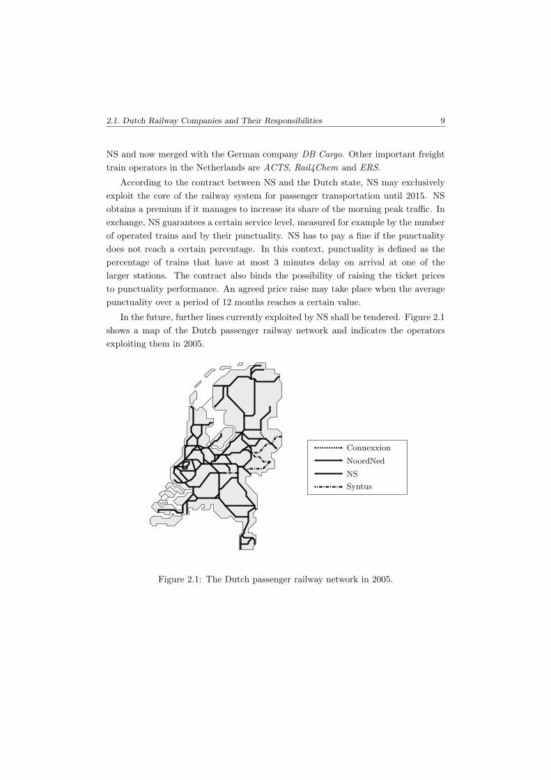
In the future, further lines currently exploited by NS shall be tendered. Figure 2.1
shows a map of the Dutch passenger railway network and indicates the operators
exploiting them in 2005.
Connexxion
NoordNed
NS
Syntus
Figure 2.1: The Dutch passenger railway network in 2005.
10 Chapter 2. Planning Railways in the Netherlands
2.1.3 The Structure of Nederlandse Spoorwegen1
NS is the largest passenger operator in the Netherlands. In 2004, NS ran about 2,800
passenger carriages with a total capacity of 265,000 seats on a rail network of about
2,800 km. With more than 20,000 employees NS is one of the largest employers in
the Netherlands.
The timetable of a day contains about 4,700 services, operating on over 100 train
lines. These timetable services connect 388 stations. About 1,000,000 passenger
journeys on a working day contributed to over 14 milliard passenger-kilometres for
the whole year. In 2004, NS reached a 3-minutes arrival punctuality of 86.0%. An
internationally accepted performance measure is the 5-minutes arrival punctuality:
it was 92.6%, in Europe only eclipsed by the Swiss Railways.
In order to see the value of these punctuality data, it is worth mentioning that the
track utilisation of the Dutch railway network is the highest in Europe. In 2002, NS
realised a ratio of 49.4 train kilometres per network kilometres. Switzerland, having
the second busiest network in Europe, reached a ratio of about 42 train kilometres
per network kilometres (Poort (2002)).
NS is divided into several parts. In this thesis we only refer to three of them that
are directly involved in rolling stock planning.
NS Reizigers or NSR (NS Passengers) is responsible for operating the trains
themselves. It plans the timetable and schedules the rolling stock as well as the
crew. Furthermore, NSR is responsible for carrying out these plans. The problems
that we consider in this thesis arise in rolling stock planning and operation at NSR.
NS Commercie (NS Commerce) is the marketing and sales department of NS. It
connects the company to the customers. It is responsible among others for predict-
ing the passenger demand. Based on these forecasts, NS Commercie decides which
stations are to be connected by direct trains.
NedTrain is responsible for the quality of the rolling stock. By carrying out regular
preventive maintenance, inside and outside cleaning and safety checks, NedTrain
keeps the rolling stock available for trains. NedTrain also refurbishes rolling stock
units in order to adjust them to the changing demands and to provide more comfort
to the passengers.
Further parts of NS manage the stations and the real estate around the stations,
operate international trains, support the entire NS Group in human resource man-
agement and legal affairs, and so on.
1The facts on NS have been collected from NS Intranet (2005).

2.2. Planning Process at NSR 11
2.2 Planning Process at NSR
The steps of the railway planning process can be classified in several ways. A com-
mon criterion is the length of the planning horizon. Based on this, one usually distin-
guishes strategic, tactical, operational and short-term planning phases (see Anthony
(1965)). This hierarchy in time also means that the products of a planning phase
serve as input for later phases where the earlier decisions may be revised according
to updated information.
Strategic planning has a planning horizon of several years or even decades, the
main focus is on capacity planning.
Tactical planning allocates the available capacity with a planning horizon of 2
months up to a year.
Operational planning sets up the fully detailed plans, the planning horizon varies
from 3 days to 2 months. Mainly, it concerns adjusting the tactical plans to
the forthcoming weeks.
Short-term planning comprises problems that arise when the actual train opera-
tions take place or just before that. It covers planning steps with a planning
horizon of at most 3 days.
These planning phases are discussed in detail later in this chapter.
Planning steps are also grouped based on their target: they belong to timetabling,
rolling stock scheduling or crew scheduling.
Finally, a third way to classify planning steps is to distinguish central and local
planning. Central planning steps affect the entire railway network, such decisions are
made at the Logistics Department of NSR in Utrecht. Local planning steps have an
impact only on a single station. For example, platform assignment is a local planning
step. Local planning steps related to rolling stock are carried out by shunting planners
and by the Transportbesturingsorganisatie2 (TBO), which is a department of NSR.
Local crew planning is arranged by planners located at the 29 crew depots.
In the next few sections, we first describe the rolling stock and human resources of
NSR. Subsequently, we give an overview of each planning phase in detail by gather-
ing planning steps of timetabling, rolling stock scheduling and crew scheduling that
belong to the planning phases. Thereafter, we have a closer look at the shunting
2Transport Control Organisation.

12 Chapter 2. Planning Railways in the Netherlands
process. Finally, we point out some features that distinguish NSR from other rail-
way companies. These special features explain why operations research models and
methods in the literature are not (or hardly) applicable to instances of NSR.
2.2.1 Rolling Stock and Human Resources
NSR operates most trains by electrical and diesel units. A unit consists of a number
of carriages, it is supplied with an engine and has driver’s cabins on both ends. The
number of carriages in a unit only indicates its length and seat capacity for first and
second class passengers. Units cannot be split up in everyday operations.
Units are available in several types. Units of the same type have identical technical
characteristics such as length or seat capacity. When functioning properly, they
are only distinguished by the number of kilometres they travelled since their last
preventive maintenance check. Some types are compatible: units of compatible types
can be combined to form a longer train, while units of incompatible types cannot.
For example, “Koploper-3” and “Koploper-4” form a pair of compatible types (see
Figure 2.2). These two types contain units with 3 and units with 4 carriages and are
mainly used for inter-city services.
Figure 2.2: “Koploper” units with 3 carriages and with 4 carriages.
Shorter units have higher costs per seat, while longer units may lead to inefficient
rolling stock usage. Having different unit lengths enables one to create compositions
whose capacity better matches the passenger demand. For example, “Koploper”
units can form a train with 3, 4, 6, 7, 8, 9, 10, 11, 12, 13, 14 or 15 carriages.3
Currently, NSR uses about 590 units of 17 types. The length of the units ranges
from 2 to 6 carriages, adding up to over 2,000 carriages in the units. There are single-
deck and double-deck units. Some types are designed for inter-city or inter-regional
trains, other types are more appropriate for regional trains. Each type is compatible
with at most one other type. The largest type of NSR is the “Mat64-2”: NSR uses
167 pieces of these two-carriage units for regional trains. Note that NSR also operates
3Due to safety regulations and platform lengths, trains of NSR may contain no more than 15carriages.

2.2. Planning Process at NSR 13
about 830 locomotive-hauled railway carriages and 120 locomotives. However, the
planning problems considered in this thesis arise when scheduling the units.
The crew scheduling problems of NSR concern train drivers and conductors, they
are the most important operational human resources for NSR. In 2005, NSR em-
ployed about 2,800 drivers and about 3,100 conductors divided into 29 crew depots.
Each driver and conductor starts and finishes the daily duty at his/her depot.
2.2.2 Strategic Planning
Strategic planning concerns decision making several years in advance. It sets the
target performance and service quality. Moreover, strategic planning makes sure
that there are enough resources to achieve these goals. The most visible strategic
decision is to determine the basic shape of the timetable by setting the train lines.
Stochastic considerations play an important role in forecasting the future passen-
ger demand as well as the long-term availability of the required resources. Strategic
planning entirely belongs to central planning.
Strategic Timetabling
The passenger demand is estimated for the forthcoming years. At this very first point
of the planning process, the origin-destination matrix is determined: it specifies the
estimated number of passengers on a day between each pair of stations.
Based on these forecasts, the train lines are determined. A train line is a series
of trains that directly connect given stations. In the Netherlands, train lines are
of three types: regional train lines with trains calling at every station along their
path; inter-regional train lines where trains do not call at the smallest stations; and
inter-city train lines where trains usually call only at major stations. Train lines have
given frequencies, e.g. once or twice per hour.
Example. The 3000 line is an inter-city train line, connecting
Nijmegen (Nm) to Den Helder (Hdr). Trains of the 3000 line call
at Nijmegen, Arnhem (Ah), Ede-Wageningen (Ed), Utrecht (Ut),
Duivendrecht (Dvd), Amsterdam Amstel (Asa), Amsterdam Cen-
traal (Asd), Alkmaar (Amr), Den Helder as well as at each station
between Alkmaar and Den Helder (see Figure 2.3). The 3000 line is
operated twice an hour in both directions.
Determining line systems means balancing several conflicting criteria. For in-
stance, long train lines provide convenient service for many passengers. On the other

14 Chapter 2. Planning Railways in the Netherlands
Hdr
Amr
AsdAsa Dvd
UtEd
Ah
Nm
Figure 2.3: The 3000 line connecting Nijmegen (Nm) to Den Helder (Hdr).
hand, they are sensitive to delays and disturbances and they often lead to less ef-
ficient rolling stock schedules. Line planning is carried out by NS Commercie and
NSR together.
One of the difficulties of line planning is the fact that passenger behaviour is very
difficult to model: It has a strong stochastic character. Moreover, demand for seats
depends on the line system: appealing new train connections may attract passengers
who otherwise would have taken their cars.
Usually, the line system does not change much for years. In 2007, however, deeper
changes are expected due to three on-going infrastructure development projects that
will have been finished by that time: the High Speed Line, connecting Amsterdam to
Rotterdam and further to Brussels and Paris; the “Utrechtboog” that allows direct
train traffic between Schiphol Airport and Utrecht; and doubling the tracks between
Amsterdam and Utrecht.
Strategic Rolling Stock Planning
Strategic rolling stock planning aims at determining the number of units needed to
cover passenger demand in the forthcoming years. It has the longest horizon among
all planning steps of NSR. It takes years until newly ordered units are actually
delivered. The expected service time of the units amounts to decades. Strategic

2.2. Planning Process at NSR 15
decisions on rolling stock concern large amounts of money and they determine the
train traffic and the service quality for years.
The basic decisions are purchasing or leasing new rolling stock and refurbishing
existing units. Redundant units may be sold or disassembled. Another problem is
to set the strategy for regular preventive maintenance. More frequent maintenance
probably results in more reliable rolling stock, decreasing the disturbances caused
by defect units. On the other hand, it also leads to higher maintenance costs and it
requires a higher number of units in use.
Strategic Crew Planning
Crew planning on the strategic level aims to provide enough train drivers and con-
ductors for the forthcoming years. This can be achieved by hiring new crew members
or by internal trainings. Train drivers and conductors start and finish their daily du-
ties at their home depot. Thus strategic crew planning also involves decisions on the
depots themselves: on opening or closing depots and on dividing the work among the
depots. Firing employees is no option at the moment, as crew members have a work
guarantee until 2010. Similarly to rolling stock planning, it takes a few years until
strategic crew planning measures have an effect: the training to become a conductor
takes about a year and to become a driver takes about two years.
2.2.3 Tactical Planning
Tactical planning at NSR refers to a planning horizon ranging from 2 months to 1
year. The output of tactical planning consists of the tactical timetable, the tactical
rolling stock schedule and the tactical crew schedule; they are planned for a generic
week of the year. Tactical planning has a bit of an operational character too, since
its products take many details of reality into account.
Tactical Timetabling
Like many European railway operators, NSR has a cyclic timetable, the cycle time
is 60 minutes. The timetable of every hour is basically the same, the daily timetable
is obtained by carrying out this pattern repeatedly.
Tactical timetable planning is carried out by central planners. It takes the previ-
ously determined line plan and estimated passenger demand as input. Moreover, the
specification contains marketing aspects like providing appealing train connections
to the passengers.

16 Chapter 2. Planning Railways in the Netherlands
The first timetabling step is to create the Basic One-Hour Pattern which describes
the departure and arrival times of the trains assuming that the timetable of each
hour is identical. Then the one-hour pattern is extended to a one-day timetable by
distinguishing peak hours, off-peak hours and night hours. Finally, adjusting the
one-day timetable to the different demands on different days of the week yields a
timetable for a generic week4.
In the timetabling phase, the rolling stock and crew is not considered explicitly
yet. The limited infrastructure capacity of stations is taken into account as follows.
Based on a draft timetable, local planners set up the Platform Occupation Charts
that assign the timetable services to the platforms. Difficulties in creating the Plat-
form Occupation Charts are reported to the central planners who update the draft
timetable accordingly.
We have seen in Section 2.1.1 that ProRail supervises and coordinates the time-
tables of the railway operators. To that end, NSR sends its timetable of a generic
week to ProRail and modifies it if ProRail requests seriously motivated changes.
Timetabling receives feed-back also from rolling stock planning at later stages of the
planning process, leading to slight adjustments of the timetable. However, these
modifications are undesirable because the new timetable has again to be checked
with ProRail.
Tactical Rolling Stock Planning
Once the timetable is known, the rolling stock has to be scheduled to carry out the
timetable services. The rolling stock schedules have two parts: the centrally planned
tactical rolling stock circulations that describe the assignment of available rolling
stock to the timetable services and the locally created tactical shunting plans that
specify the train movements inside the stations. (We discuss the shunting process in
Section 2.2.6.)
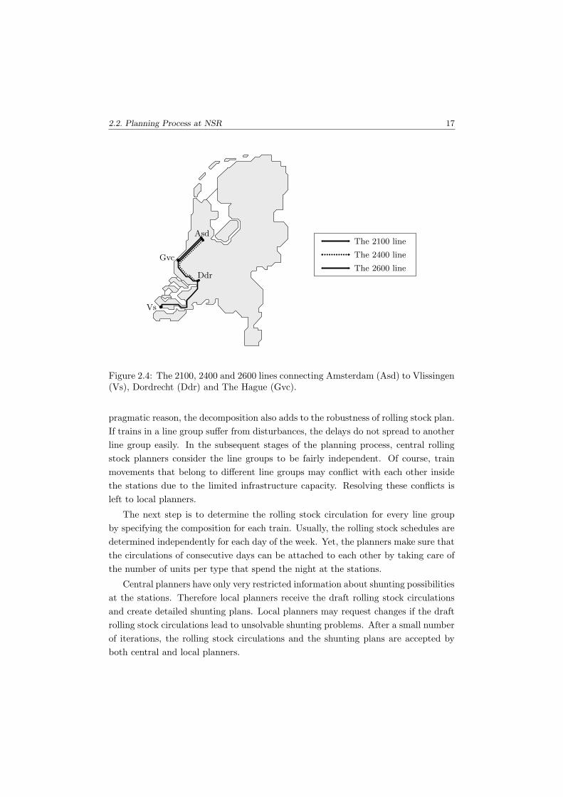
The first step is to assign the available rolling stock to the so-called line groups: A
line group is the collection of interconnected lines. For example, the 2100, 2400 and
2600 lines connecting Amsterdam (Asd) to Vlissingen (Vs), Dordrecht (Ddr) and The
Hague (Gvc) form a line group (see Figure 2.4). The 3000 line in itself forms another
line group. According to the current planning strategy of NSR, rolling stock is bound
to line groups as much as possible: a daily workload of a unit preferably contains only
trains that belong to the same line group. The reason for this decomposition is that
otherwise the rolling stock scheduling problems would be far too large. Besides this
4Passenger demand on Tuesday, Wednesday and Thursday are very similar, therefore these threedays get nearly identical schedules in tactical planning.
2.2. Planning Process at NSR 17
Asd
Gvc
Ddr
Vs
The 2100 line
The 2400 line
The 2600 line
Figure 2.4: The 2100, 2400 and 2600 lines connecting Amsterdam (Asd) to Vlissingen(Vs), Dordrecht (Ddr) and The Hague (Gvc).
pragmatic reason, the decomposition also adds to the robustness of rolling stock plan.
If trains in a line group suffer from disturbances, the delays do not spread to another
line group easily. In the subsequent stages of the planning process, central rolling
stock planners consider the line groups to be fairly independent. Of course, train
movements that belong to different line groups may conflict with each other inside
the stations due to the limited infrastructure capacity. Resolving these conflicts is
left to local planners.
The next step is to determine the rolling stock circulation for every line group
by specifying the composition for each train. Usually, the rolling stock schedules are
determined independently for each day of the week. Yet, the planners make sure that
the circulations of consecutive days can be attached to each other by taking care of
the number of units per type that spend the night at the stations.
Central planners have only very restricted information about shunting possibilities
at the stations. Therefore local planners receive the draft rolling stock circulations
and create detailed shunting plans. Local planners may request changes if the draft
rolling stock circulations lead to unsolvable shunting problems. After a small number
of iterations, the rolling stock circulations and the shunting plans are accepted by
both central and local planners.

18 Chapter 2. Planning Railways in the Netherlands
The major criteria in railway planning are efficiency, service quality and reliability.
In tactical rolling stock planning, they refer to cutting operational costs by reducing
carriage-kilometres, to providing enough seat capacity on the timetable services and
to keeping the number of composition changes low. Further details about tactical
planning are given in Chapter 3 that deals with the tactical rolling stock circulation
problem.
In the tactical phase, units are not considered as individuals yet. Instead, duties
are determined for anonymous units: A duty is the daily workload of a unit. The
duties are assigned to individual units in the short-term planning phase, a couple of
days before actually carrying out the duties. The tactical shunting plans determine
the successive duty of each duty that is to be carried out by the same particular unit
on the next day. However, these night transitions are not very binding; they serve
much more as a capacity check so that the rolling stock schedules of two consecutive
days fit together.
Tactical Crew Planning
Crew scheduling is divided into two parts. First, it consists of generating the duties
for train drivers and conductors, where a duty is a daily workload of an anonymous
employee. Thereafter, the duties on different days are composed to rosters. Gen-
erating the duties is a central planning task, while rostering is carried out by local
planners at the crew depots.
When creating the daily duties, the main objective is to minimise the number
of needed duties subject to a large number of requirements. Examples of natural
restrictions include the requirement that every train should have a driver and a given
number of conductors and that the driver of a train must know both the trajectory
and the rolling stock type. Other requirements are based on agreements with trade
unions. They include restrictions on the duties themselves: a duty may not be longer
than 9 hours, it must contain a meal break longer than 30 minutes, and so on. Finally,
there are global constraints on the schedule. For example, there is a bound on the
average time duration of the duties per depot and the workload is to be distributed
among the depots as fairly as possible. Note that crew scheduling takes the rolling
stock schedules as input. One of the reasons for this is that the number of needed
conductors depends of the length of the train.
The second step in crew planning is rostering : the daily duties are composed
to chains of duties, each chain is to be assigned to a crew member. Duties have
different characteristics like early duties, night duties or long duties. The chain must
fulfil complex requirements, making sure that the employees get enough rest. For
2.2. Planning Process at NSR 19
example, a sequence of at least 3 night duties must be followed by a rest period of
at least 48 hours. Another rule requires that each employee has a fully free weekend
at least once in every 3 consecutive weeks.
Crew rostering is one of the few tactical planning steps whose products may not
be changed in the operational planning phase. In short-term planning, however, the
crew rosters often need adjustments.
2.2.4 Operational Planning
In this thesis, the term operational planning is used for planning tasks with horizons
of 3 days up to 2 months. In operational planning, the generic week plan (i.e. the
result of tactical planning) is adjusted to the specific demands of the particular weeks.
Reasons for such adjustments can be the need for extra trains because of cultural
or sports events, national feasts, and so on. Another reason is the unavailability
of railway tracks because of maintenance. In particular, the unavailability of tracks
may require large-scale adjustments. At NSR, most effort in operational planning is
spent for these larger adjustments. The usual duration of infrastructure maintenance
works is 1–2 days (mostly in the weekend), but they may also take a couple of weeks.
The operational planning steps themselves are similar to those in tactical plan-
ning, but the main focus differs. Tactical plans are intended to minimise objective
criteria that directly translate to operational costs and service quality. Since the
horizon of typical operational planning problems is relatively short, efficiency is no
longer the main objective. Much more important is to come up with the adjusted
plans quickly and to make sure those plans can be carried out smoothly. As we have
seen in the previous section, several rounds of information exchange between central
planners, local planners and ProRail are required to make them agree on the tactical
plans. This agreement is also necessary for the operational modifications. Therefore
the tactical plans have to be modified in such a way that central and local planners
can agree on the adjustments quickly.
The products of operational planning are the operational timetable, the opera-
tional rolling stock schedule and the operational crew schedule. A couple of days
before the operational plans are to be carried out, they are transferred to the traffic
control offices of ProRail and to TBO (cf. Section 2.2.5). From then on, they are
responsible for adjusting the operational plans to the real-time events.

20 Chapter 2. Planning Railways in the Netherlands
Operational Timetabling
The tactical timetable is updated by inserting or deleting trains and by modifying the
arrival and departure times of existing ones. In case of infrastructure maintenance,
the updated timetable must obey the altered infrastructure availability. Also, the
operational timetable has to be approved by ProRail.
Operational Rolling Stock Planning
Similarly to the tactical rolling stock schedules, the operational rolling stock schedules
have two parts: the centrally planned operational rolling stock circulations and the
locally created operational shunting plans.
Central planners take the shunting possibilities into account in a similar way as
they do in tactical planning. The draft operational rolling stock circulations are sent
to the local planners who try to create the corresponding detailed shunting plans
and require modifications if necessary. Similarly to tactical planning, the operational
rolling stock schedules consider duties for anonymous units.
Usually, minor modifications of the tactical plans are handled easily. Much more
effort is needed in case of infrastructure maintenance. Then planners at NSR apply
the following two-phase method. First, they set up an intermediate plan that meets
requirements except for the initial inventories. The initial inventory of a station is the
number of units per type that start there at the beginning of the planning horizon.
So, it can happen that 3 units are available at a station prior to the infrastructure
maintenance, while the intermediate plan requires 4 departing units at the beginning
of the planning horizon; then the station has an off-balance. A quick planning process
requires that the intermediate plan is very likely agreed on by local planners. To
achieve this, the intermediate plan contains as few underway composition changes
as possible. The second phase resolves the off-balances by additional modifications.
This two-phase method is discussed in detail in Chapter 5.
Operational Crew Planning
Operational crew planning means adjusting the duties in the tactical crew sched-
ule by central planners. Tactical crew rosters were created to fulfil complex rules
during the forthcoming months and the employees know their working times several
weeks ahead. Changing the rosters would make their working times unpredictable.
Therefore the crew rosters may not change in operational planning. Instead, the op-
erational crew planners try to modify the daily duties of the drivers and conductors,
while maintaining the number of duties and their characteristics such as early starting

2.2. Planning Process at NSR 21
duties, night duties, and so on. Thereby the modified duties remain compatible with
the crew rosters. Again, in contrast to tactical planning with the number of duties
as the main objective, operational planning is much more a feasibility problem.
2.2.5 Short-term Planning
Short-term planning is the last phase of railway planning, it amounts to making
decisions with a horizon of at most 3 days. In particular, it includes real-time reacting
to the latest developments. The operational plans are transferred to the traffic control
offices and to TBO 3 days before carrying them out. From that point on, the traffic
control offices, being part of ProRail, are responsible for the timetable, while TBO
is responsible for adjusting and executing the operational rolling stock and crew
schedules. So, most short-term planning steps are local. Yet, there are some aspects
that require central coordination.
In short-term planning problems, there is not much time for computations in
order to get the best possible solutions. Mostly, any feasible solution which keeps
the railway system moving is good.
Short-term Timetabling
The most important task is delay and disruption management. The infrastructure
capacity has been divided between the operators. However, the operators may not
be able to run their trains on time due to disturbances. The traffic control offices,
which are part of ProRail, decide in which order the delayed trains may enter the
stations and the trajectories.
Short-term Rolling Stock Planning
Short-term rolling stock planning is carried out by TBO which is divided into a
central and a local part. The central part of TBO is called Materieelregelcentrum5
(MRC). The planning tasks are shared between the parts of TBO as follows.
The operational plan describes daily duties but not the assignment of duties to
particular units. This is done by local planners of TBO. They can do this arbitrarily
as long as each duty gets a unit of the type it was planned for.
When carrying out the operational rolling stock schedules, delays or disruptions
may occur. Then TBO must react to provide rolling stock for the timetable services.
However, lack of instantly available rolling stock at the right place often may lead
5Rolling Stock Management Centre.
22 Chapter 2. Planning Railways in the Netherlands
to additional delays or even cancellation of trains. A special form of disruption
management is to keep track of type mismatches. Time to time, local planners are
forced to fill duties with a “wrong” type. Central planners at MRC have a global view
of the rolling stock circulations and they try to correct the mismatches by sending
instructions to the local planners. As in earlier phases, each change of the rolling
stock plan must be approved by local planners.
An important issue in short-term rolling stock management is maintenance. Units
need regular preventive check-ups. Each unit must undergo a small safety inspection
every 48 hours. Since such inspections can take place basically at every shunting
yard, it is part of the shunting process. However, units also need more involved
maintenance checks, say every 30,000 km: Units that travelled that far since their
previous maintenance check must go to a maintenance facility. This is arranged by
maintenance routing planners at MRC. So, maintenance routing is a central plan-
ning step. On every day, the units with the highest number of kilometres since their
last maintenance check are listed, these units are called urgent . They must undergo
maintenance in the forthcoming 3 days. Maintenance routing planners modify the
operational rolling stock schedules so that the urgent units are routed to the main-
tenance facilities. Being that close to executing the operational plans, there is no
time to come up with completely new rolling stock schedules. Instead, small and
localised exchanges are applied, for example by swapping two units of the same type.
Maintenance routing is discussed in detail in Chapter 4.
Short-term Crew Planning
Short-term crew planning is a task of TBO, too. The main task is to handle disrup-
tions. Each train must be supplied with a driver and a given number of conductors.
If this is not possible because of disturbances of the railway system, the train has to
be delayed or even cancelled.
2.2.6 Shunting
Shunting refers to all train movements inside the stations. As one could see in the pre-
vious sections, shunting is an important issue in every phase of rolling stock planning.
This thesis does not deal with the shunting problem explicitly. Nonetheless, shunting
considerations play an important role in each model of the subsequent chapters. The
two most significant elements of shunting are routing trains through a station and
positioning temporarily not used units to the shunting yards.

2.2. Planning Process at NSR 23
In the daytime, the passing trains need a free platform to let the passengers
get in and out of the train. Moreover, they must be routed through the stations
in such a way that they do not block the paths of each other. Sometimes, the
compositions must be adjusted to the passenger demand by coupling units to the
trains or uncoupling units from them. This happens often just before and just after
peak hours when the number of passengers increases or decreases. Since the timetable
of NSR is very dense, the stations provide only a restricted capacity to change the
compositions. On the other hand, composition changes are potential sources for
delays, therefore they are to be avoided as much as possible.
At night, the units are to be stored in such a way that the start-up on the next
morning requires the smallest possible number of shunting movements. Implicitly, it
includes assigning the units arriving in the evening to rolling stock duties starting
next morning. Moreover, units have to be cleaned every day and they must undergo
a small technical check on every second day.
The shunting process is arranged by local planners located at several major sta-
tions. Solving the shunting problem itself is quite a challenging task, even for a single
day and for a single middle-sized station. Therefore, central planners must rely on
the knowledge of the local planners throughout the entire planning process.
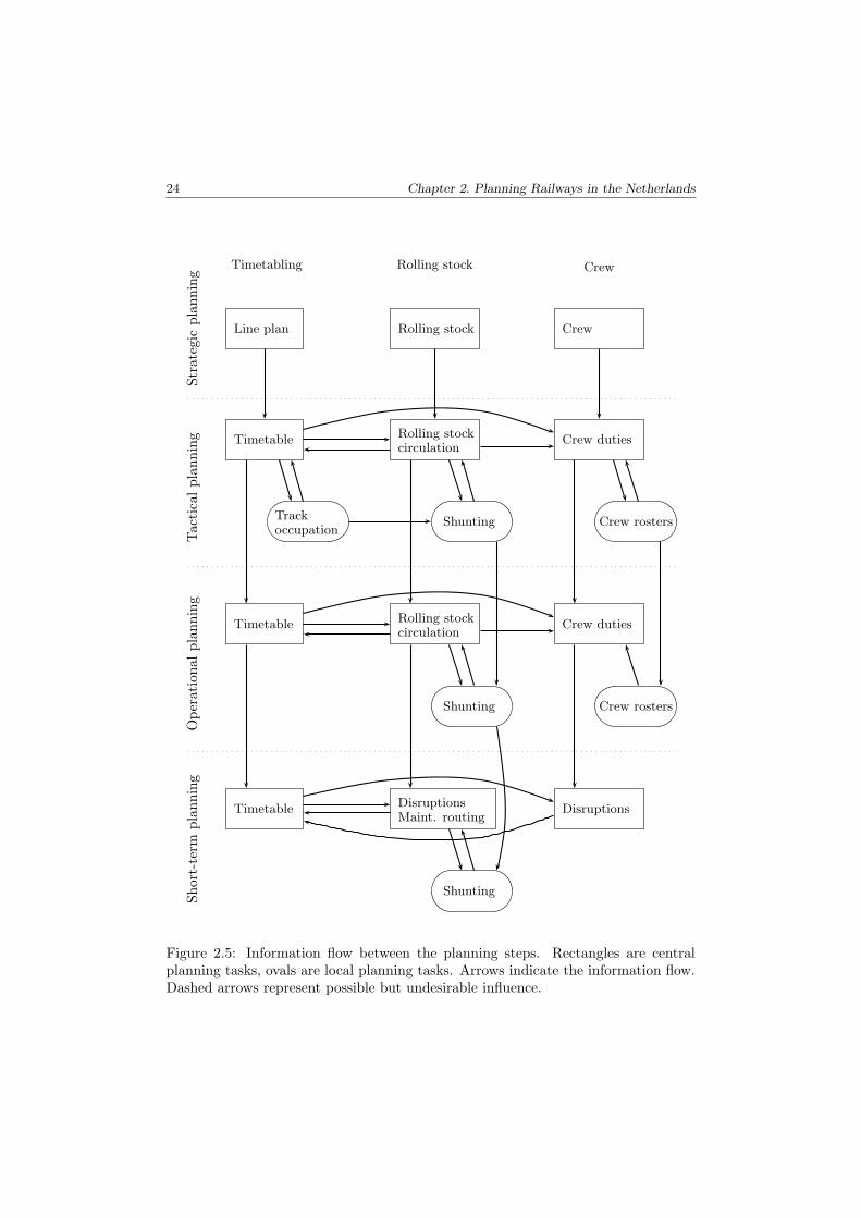
2.2.7 Information Flow between the Planning Phases
As we have seen in the previous sections, the planning steps interact in a quite
complex way. We give an intuitive overview of the most significant interactions
in Figure 2.5. Rectangles indicate central planning tasks and ovals indicate local
planning tasks. The arrows show the information flows. Dashed arrows are drawn
when the influence of a planning step to another is possible but undesirable.
Note that reality is more complex than the figure indicates. Occasionally, planning
tasks may have an influence on each other even if no according arc is drawn in
Figure 2.5. For example, tactical and operational crew planners may request changes
in the timetable if they are unable to create the crew duties. However, any feed-back
of these kinds is much more an exception than a rule.
2.2.8 Special Features of NSR
Heavily Utilised Railway System
The most peculiar property of the Dutch railway network is its heavy workload.
In 2004, NSR realised 115,000,000 train-kilometres on a network of 2,800 kilometres.
24 Chapter 2. Planning Railways in the Netherlands
Timetabling Rolling stock Crew
Str
ateg
icpla
nnin
g
Line plan Rolling stock Crew
Tac
tica
lpla
nnin
g Timetable
Trackoccupation
Rolling stockcirculation
Shunting
Crew duties
Crew rosters
Oper
atio
nal
pla
nnin
g
Timetable Rolling stockcirculation
Shunting
Crew duties
Crew rosters
Shor
t-te
rmpla
nnin
g
Timetable DisruptionsMaint. routing
Shunting
Disruptions
Figure 2.5: Information flow between the planning steps. Rectangles are centralplanning tasks, ovals are local planning tasks. Arrows indicate the information flow.Dashed arrows represent possible but undesirable influence.
2.2. Planning Process at NSR 25
Some tracks between major cities are so heavily used that often the 3-minutes security
headway between the trains prevents planners to insert additional trains.
A consequence of this is that stations have a large throughput. When a train
arrives at a station, it may depart soon as another timetable service, we call this
a turn-around . Also, the arriving units may be put to a shunting yard and used
again only a couple of hours later. In any case, the arrival platform must be freed
up as soon as possible, allowing another train to arrive. Heavy traffic often restricts
the possibilities to adjust the compositions during the turn-arounds. In fact, it is
preferred that no composition change happens at all. However, this may result in
either an inefficient schedule or high seat shortages.
A busy timetable also leads to short turn-around times making sure that the
platforms become free as soon as possible. Also, all rolling stock is needed during
peak hours: a long turn-around simply occupies rolling stock without using it to
carry passengers. The turn-around times at NSR range from about 5 minutes to
about 30 minutes.
Rolling Stock
Unlike most railway operators, NSR mainly uses units instead of locomotive-hauled
carriages. Having a driver’s seat on both ends of units allows a fast and easy turn-
around process in case of direction changes. Also, the shunting process for self-
propelled units is easier than for locomotive-hauled carriages.
Units containing different numbers of carriages can be combined to compositions
of various lengths in order to match passenger demand. However, multiple types in
a train force one to consider the order of the units in the composition, not only their
number. For example, ‘334’ and ‘343’ are both compositions with two “Koploper”
units of length 3 and with one unit of length 4, but they provide different possibil-
ities for composition changes. The unit of length 4 lies on the right hand side of
composition ‘334’, it may be possible to uncouple it, resulting in a composition ‘33’.
Composition ‘343’, however, contains the unit of length 4 in the middle, therefore
much more effort is required to uncouple it; in practise it is virtually impossible.
Successor Trains
We mentioned in Section 2.2.3 that the line system is divided into line groups and that
a unit is basically bound to a line group during a day. The decomposition into line
groups turns rolling stock planning into subproblems of tractable size. Furthermore,

26 Chapter 2. Planning Railways in the Netherlands
a rolling stock schedule with units bound to line groups is expected to be less sensitive
to disturbances and delays.
A unit that arrives at a station in a train can continue its daily duty in several
trains departing from that station. By the short turn-around times and the line
groups, arriving units usually go over to the earliest departing train that belongs to
the same line group. We call it the successor train of the arriving train. The arriving
train itself is the predecessor of its successor train.
We emphasise that it may be possible to adjust a composition during a short
turn-around. Units can be uncoupled and placed to a shunting yard, or other units
that have been stored at the station may be added to the train before departure.
The layout of the station determines in most cases at which end of the composition
this is possible.
Some in-coming trains have no successor trains. This happens mostly to trains
that arrive in the evening. Their units are supposed to go directly to the shunting
yards, to be used a couple of hours later or the next day. Similarly, early departing
trains do not have predecessors.
At NSR successor trains are specified as early as at the beginning of the tactical
planning phase. In many versions of the rolling stock circulations problem in the
literature and at other railway companies, determining the successor trains is part of
the problem.
Splitting and Combining Trains
Trains have usually at most one successor and at most one predecessor. However,
NSR operates some lines where timetable services are split and combined. For exam-
ple, the 1600 line contains services from Enschede to Amsterdam and from Enschede
to Schiphol: the trains from Enschede are split in Amersfoort, the front part depart-
ing to Amsterdam, the rear part departing to Schiphol. On the way back, trains
from Amsterdam and Schiphol arrive at Amersfoort to be combined and to depart a
couple of minutes later towards Enschede (see Figure 2.6).
Note that we only speak about splitting if the successor trains depart within a
couple of minutes after their predecessor train arrived. We distinguish splitting from
the case when units are simply uncoupled during a turn-around. When a train is split,
the exact composition of both split parts must be carefully identified. However, the
order of uncoupled units on the shunting yards does not matter much as the shunting
crew has usually enough time later to carry out necessary shunting movements. A
similar restriction applies for combining trains.

2.3. Operations Research in Railway Planning 27
Asd
Shl AmfDv Es
Figure 2.6: The 1600 line.
Splitting and combining occurs very often in the so-called Noord-Oost line group,
an interconnected system of inter-city lines of NSR. Largely due to the complications
caused by splitting and combining, the Noord-Oost line group is considered to be the
hardest instance among all rolling stock circulation problems of NSR.
2.3 Operations Research in Railway Planning
Optimisation of railway transportation has always been an intensively investigated
topic in operations research6. Surveys such as by Assad (1980) and by Cordeau et al.
(1998) consider the entire spectrum of railway planning, from infrastructure related
questions through problems at passenger and freight operators. Since this thesis deals
with problems that arise at NSR, we restrict ourselves here to research questions of
passenger railway operators. Even then, the literature list is not intended to be
complete. An exhaustive overview of the topic falls out of scope of this thesis. We
also refer to a recent survey of Huisman et al. (2005) on operations research methods
in passenger railway transportation, with a special focus on planning problems of
NSR.
6Moreover, one of the first applications of the famous Max Flow Min Cut theorem was to in-vestigate how to destroy the enemy’s railway system as efficiently as possible (see Schrijver (2003)p. 168).

28 Chapter 2. Planning Railways in the Netherlands
In the next few sections, we list a number of publications and successful operations
research applications in railway planning. We structure the literature overview in the
same way as we classified the planning steps in the previous sections.
2.3.1 OR Methods for Strategic Planning
Timetabling
The most important research problem here is line planning. Goossens (2004) provides
an overview of this topic, focusing mainly on efficiency improvement for railway
operators. Bussieck (1998), Scholl (2001) and Scholl (2005) describe methods to
optimise customers’ convenience of the line system, by providing as much direct
connections as possible or by minimising the number of transfers.
Rolling Stock and Crew
Although long-term rolling stock and crew management concern significant amounts
of money and have major consequence for the service quality for years or decades,
they have received less attention in the operations research literature than tactical or
operational planning. A reason for this is the difficulty to forecast the future demand
for resources.
Strategic planning models must be able to deal with uncertain factors. Therefore
the natural approach is stochastic optimisation. Recently, Van Dijk (2003) developed
a model for strategic crew management. The model makes suggestions for hiring
or internal training of employees, taking among others the fluctuating number of
employees and their unavailability due to training, vacation or illness into account.
2.3.2 OR Methods for Tactical Planning
Among all phases of the railway planning process, tactical planning attracted the
most attention in the operations research literature. Cyclic (and non-cyclic) time-
tabling, rolling stock circulations and crew scheduling are discussed in many publica-
tions. The research resulted in several software packages that became indispensable
planning tools of the railway companies.
Timetabling
Cyclic timetabling is an intensively researched topic. Peeters (2003) describes this
problem in detail with an extensive list of references. Another important and difficult
2.3. Operations Research in Railway Planning 29
problem is to evaluate the quality of a timetable. One of the major objectives is
robustness: the timetable should allow high overall punctuality even when there are
disturbances. Robustness is a requirement at the network level that is very difficult
to express in terms of the decision variables used in timetabling models. Instead,
simulation and stochastic analysis tools are used to compare given timetables.
ProRail and NSR make use of the software package DONS 7 (see Hooghiemstra
(1996), Hooghiemstra et al. (1999), Schrijver and Steenbeek (1994) and Zwaneveld
et al. (1996)). ProRail uses DONS primarily to analyse the effect of infrastructure
extensions on timetables. Within NSR, DONS is used to determine the basic shape
of the timetables in the near future.
The simulation software SIMONE has been developed for ProRail and NSR to
analyse the sensitivity of timetables to disturbances and delays. Vromans and Kroon
(2004) and Vromans et al. (2005) describe quantitative methods to evaluate and
optimise the robustness of timetables. State-of-the-art results in this topic are sum-
marised in Vromans (2005).
Rolling Stock
The first step in tactical rolling stock planning at NSR is to allocate the rolling stock
to the line groups. Abbink et al. (2004) describe a model for this problem. The
main criterion is to minimise the seat shortages during the morning peak hours and
to minimise the number of different rolling stock types per line group. This model is
currently used at NSR to divide the rolling stock among the line groups.
Rolling stock circulation has been addressed in quite a few papers. For example,
Schrijver (1993), Ben-Khedher et al. (1998), Brucker et al. (1998), Cordeau et al.
(2000), Cordeau et al. (2001a), Alfieri et al. (2002), Lingaya et al. (2002) and Peeters
and Kroon (2003) deal with this problem. Chapter 3 is devoted to tactical rolling
stock planning, we discuss these papers there more deeply.
Crew
Crew scheduling, especially creating crew duties, belongs to the most successful ap-
plications of operations research methods. Intensive research has lead to a major
break-through in the last couple of years.
The duty generation problem in crew scheduling can be formulated as a gener-
alised set covering problem, the decision variables express whether or not a candidate
7Designer Of Network Schedules.
30 Chapter 2. Planning Railways in the Netherlands
duty is selected. The solution method can be based on the linear programming relax-
ation or on Lagrangian relaxation. Integer solutions may be obtained by a branch-
and-price method, described for example by Barnhart et al. (1998b). Alternatively,
heuristic algorithms may be used. The algorithm described by Caprara et al. (1999)
turned out to be especially useful in practise. Since 2000, the software package
TURNI has been used at NSR to create duties for the crew. TURNI implements a
column generation framework and makes use of the heuristic algorithm of Caprara
et al. (1999). With appropriate fine-tuning, TURNI is capable to produce duties
that are accepted both by the management of NSR and by the employees. More
details about results with TURNI can be found in Kroon and Fischetti (2001) and
in Abbink et al. (2005).
Most other major European railway companies use crew scheduling software,
too. The best known packages are CARMEN (Kohl (2003), used among others at
the German Railways) and TRACKS II (Fores et al. (2001), used at several railway
companies in the United Kingdom). We also mention that similar crew scheduling
problems arise at bus and airline companies.
In contrast to crew duties, generating crew rosters fully automatically is still a
challenge. Kohl and Karish (2004) provide an overview on crew rostering methods,
mainly used in airline industry. Traditionally, most European public transportation
companies apply a special variant of rosters, so-called cyclic rosters. Recent publi-
cations on cyclic crew rostering include Caprara et al. (1998) and Sodhi and Norris
(2004).
2.3.3 OR Methods for Operational Planning
We already mentioned that tactical rolling stock and crew planning at NSR have a
certain operational flavour. Therefore, most publications on rolling stock and crew
scheduling that we cited in Section 2.2.3 are relevant here, too.
2.3.4 OR Methods for Short-term Planning
A number of papers in the operations research literature deals with short-term railway
planning problems. However, very few successful decision support tools have been
developed so far. Some recent works on dispatching public transportation systems
include Suhl and Mellouli (1999), Shen and Wilson (2001) and Suhl et al. (2001).
Although not part of the railway planning process, it is worthwhile to mention the
timetable information system applications described by Schulz et al. (2002) and by
Wagner and Willhalm (2003).

2.4. Further Aspects 31
Maintenance routing is one of the most studied short-term planning problems
in the literature. Maintenance routing problems with specifications that differ from
the problems at NSR have been described (mostly for airline applications) by Feo
and Bard (1989), Clarke et al. (1997), Barnhart et al. (1998a), Gopalan and Talluri
(1998), Talluri (1998) and Anderegg et al. (2003). Moreover, the model of Lingaya
et al. (2002) for operational rolling stock planning also incorporates maintenance.
The maintenance routing problem is discussed in detail in Chapter 4.
2.3.5 OR Methods for Shunting
Several papers in the literature address the shunting problem. Winter (1999), Winter
and Zimmermann (2000) and Blasum et al. (2000) focus on dispatching trams, Gallo
and di Miele (2001) consider the shunting problem for buses. Tomii et al. (1999)
and Tomii and Zhou (2000) describe a genetic algorithm to solve related problems.
Freling et al. (2005) and Lentink et al. (2003) seek for solution methods that can
cope with several practical issues of shunting problems at NSR. A more extensive
description of the topic is given by Lentink (2006). Despite promising computational
results, solving shunting problems remains a challenging task, even for a single day
and for a single middle-sized station.
2.4 Further Aspects
In the previous sections we listed a number of planning tasks that need to be carried
out and that are addressed to some extent by operations research techniques. Yet,
there are other aspects that can have a large influence on the entire planning process
or at least on some parts of it.
Redesigning the Planning Process
The careful reader must have realised that the planning process described in the
previous sections contains planning steps whose results will barely (or never) be used
when actually carrying out the plans. For example, the tactical rolling stock schedules
are not carried out as they are; instead, they are transformed to the operational
schedules. The operational schedules contain fully detailed shunting plans but these
are hardly ever carried out without major changes, too. New shunting plans must
often be created in the short-term planning phase in order to react to the latest
developments. Moreover, several factors that appear as late as in the short-term

32 Chapter 2. Planning Railways in the Netherlands
phase may affect the shunting plans. Such factors are maintenance routing, cleaning
and technical inspections of the units.
Planners should not need to create fully detailed rolling stock plans one year in
advance with the knowledge that a lot of the details must be revised later. Therefore
tactical planning and partly operational planning needs reliable tools to estimate
shunting capacity of the stations.
Filling in the fine details as late as possible is the basic idea of the project Heront-
werp (Redesign) of NSR. It aims at restructuring the planning process so that early
stages only focus on capacity planning but not dealing with all the details. Besides the
mentioned example of the shunting plans, Herontwerp addresses the whole spectrum
of planning questions at NSR. An important part of the project is to develop the
required capacity checking tools.
Information Systems
Computer-based decision support tools but also human planners need the appropriate
input data. Currently, central planners and local planners do not have direct access
to each other’s data. Unifying the databases, being a part of Herontwerp, is an
on-going project at NSR.
Short-term rolling stock planners are often faced with the problem that they
cannot get the exact location of a physical unit instantly. This may have several
consequences, such as slowing down the maintenance routing process. The units have
recently been supplied with GPS receivers to locate them and with GSM devices to
transmit their position and status information.
An important point in using computers as decision support tools is to display the
output in such a way that the planners can interpret the results easily. For example,
a recently developed application for visualisation of automatically generated rolling
stock circulations turned out to be crucial for the acceptance of the system and its
results by the planners.
Chapter 3
Tactical Rolling Stock
Circulations
In tactical planning, the rolling stock schedule is created for a generic week of the
year so that the schedule respects every practical requirement and so that it can be
carried out repeatedly. The schedule is composed of the rolling stock circulations and
the shunting plans. In this chapter, we discuss the rolling stock circulation problem
that arises in tactical planning.
Till recently, the tactical rolling stock circulations of NSR were created manually.
The models and results below show that the problem can be successfully treated by
operational research methods.
The chapter is organised as follows. First we formulate the problem and give
a literature overview. Then we describe two ways of modelling the tactical rolling
stock circulation problem. The first approach is the ‘Composition Model’ which is
highly related to network flows. The second approach is the ‘Job Model’ which is
a set-covering type model. We present computational results for both models on
instances of NSR.
3.1 Literature Overview
The tactical rolling stock circulation problem has been addressed in quite a few papers
in the literature. However, in many cases the problem formulation substantially
differs from the specifications of NSR. NSR uses units of several types. The restricted
shunting possibilities enforce one to consider the order of these different types in the
33

34 Chapter 3. Tactical Rolling Stock Circulations
compositions. However, models in the literature were often set up for locomotive-
hauled railway carriages whose order may not matter. Also, the problem specification
of NSR determines the successor trains described earlier. This is not always the case
in tactical rolling stock planning problems in the literature. An additional peculiarity
is that the objective function includes seat-shortage kilometres and the number of
composition changes besides the usual criterion of carriage-kilometres. Finally, no
models were developed so far to handle splitting and combining of trains.
We first discuss research results chronologically that were developed to solve in-
stances of NSR. Naturally, these are the papers most related to the topic of this
chapter.
Schrijver (1993) considers the problem of minimising the number of units needed
to satisfy the passenger seat demand for a single train line and a single day. The
method computes for every trip the number of units per type to be used, not consid-
ering the order of the units in the compositions. Seat shortages and the number of
composition changes do not appear in the objective function. The integer programs
are solved by commercial MIP solvers.
Groot (1996) and later Alfieri et al. (2002) describe an integer programming model
to determine the rolling stock circulation for multiple rolling stock types on a single
line and a single day, considering also the order of the units in the compositions.
The objective is to minimise the number of units or the carriage-kilometres such
that the given passenger demand is satisfied; seat shortages are not allowed and the
number of composition changes is not minimised. The solution methodology is to
decompose the problem into subproblems and to use their solutions to reduce the
size of the original problem, so that it becomes tractable by commercial MIP solvers.
The approach is tested on real-life case-studies of NSR.
Van Montfort (1997) presents a model for computing circulations of locomotive-
hauled railway carriages. The objective is to minimise the number of carriages and
the number of carriage-kilometres subject to given demands. The model deals with
first and second class carriages and uses a simple but realistic way to take the order
of the carriages into account. The model is solved by commercial MIP solvers.
Peeters and Kroon (2003) describe a model with exactly the same specifications
as we are considering in this chapter. They apply Dantzig-Wolfe decomposition as
solution technique. The resulting large linear program is first solved by column gener-
ation, then branch-and-price is applied to obtain integer solutions. With appropriate
fine-tuning, the approach is capable to solve real-life instances of NSR within a cou-
ple of seconds. However, the model strongly uses the fact that trains have at most
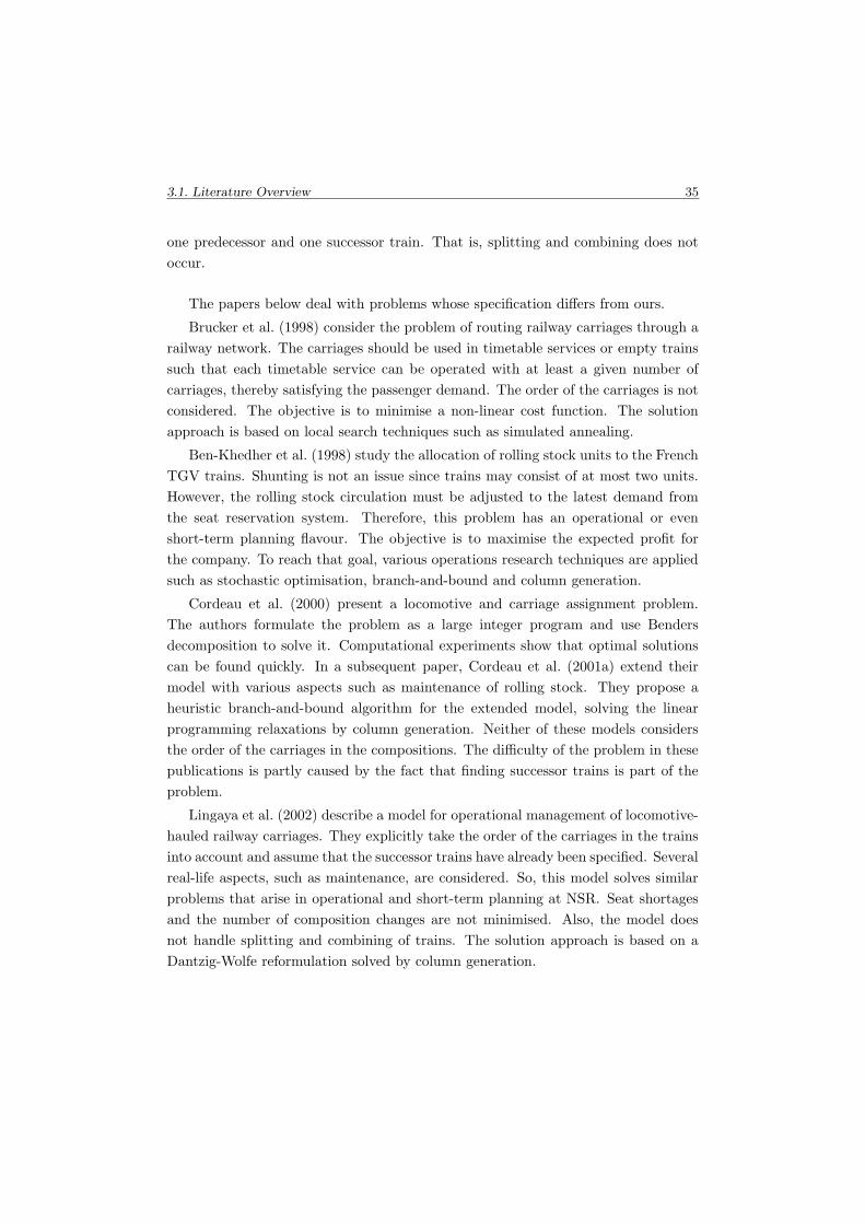
3.1. Literature Overview 35
one predecessor and one successor train. That is, splitting and combining does not
occur.
The papers below deal with problems whose specification differs from ours.
Brucker et al. (1998) consider the problem of routing railway carriages through a
railway network. The carriages should be used in timetable services or empty trains
such that each timetable service can be operated with at least a given number of
carriages, thereby satisfying the passenger demand. The order of the carriages is not
considered. The objective is to minimise a non-linear cost function. The solution
approach is based on local search techniques such as simulated annealing.
Ben-Khedher et al. (1998) study the allocation of rolling stock units to the French
TGV trains. Shunting is not an issue since trains may consist of at most two units.
However, the rolling stock circulation must be adjusted to the latest demand from
the seat reservation system. Therefore, this problem has an operational or even
short-term planning flavour. The objective is to maximise the expected profit for
the company. To reach that goal, various operations research techniques are applied
such as stochastic optimisation, branch-and-bound and column generation.
Cordeau et al. (2000) present a locomotive and carriage assignment problem.
The authors formulate the problem as a large integer program and use Benders
decomposition to solve it. Computational experiments show that optimal solutions
can be found quickly. In a subsequent paper, Cordeau et al. (2001a) extend their
model with various aspects such as maintenance of rolling stock. They propose a
heuristic branch-and-bound algorithm for the extended model, solving the linear
programming relaxations by column generation. Neither of these models considers
the order of the carriages in the compositions. The difficulty of the problem in these
publications is partly caused by the fact that finding successor trains is part of the
problem.
Lingaya et al. (2002) describe a model for operational management of locomotive-
hauled railway carriages. They explicitly take the order of the carriages in the trains
into account and assume that the successor trains have already been specified. Several
real-life aspects, such as maintenance, are considered. So, this model solves similar
problems that arise in operational and short-term planning at NSR. Seat shortages
and the number of composition changes are not minimised. Also, the model does
not handle splitting and combining of trains. The solution approach is based on a
Dantzig-Wolfe reformulation solved by column generation.
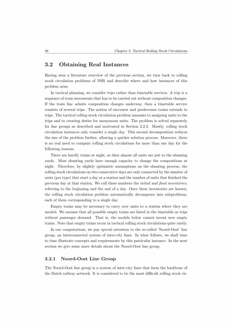
36 Chapter 3. Tactical Rolling Stock Circulations
3.2 Obtaining Real Instances
Having seen a literature overview of the previous section, we turn back to rolling
stock circulation problems of NSR and describe where and how instances of this
problem arise.
In tactical planning, we consider trips rather than timetable services. A trip is a
sequence of train movements that has to be carried out without composition changes.
If the train line admits composition changes underway, then a timetable service
consists of several trips. The notion of successor and predecessor trains extends to
trips. The tactical rolling stock circulation problem amounts to assigning units to the
trips and to creating duties for anonymous units. The problem is solved separately
for line groups as described and motivated in Section 2.2.3. Mostly, rolling stock
circulation instances only consider a single day. This second decomposition reduces
the size of the problem further, allowing a quicker solution process. Moreover, there
is no real need to compute rolling stock circulations for more than one day for the
following reasons.
There are hardly trains at night, so then almost all units are put to the shunting
yards. Most shunting yards have enough capacity to change the compositions at
night. Therefore, by slightly optimistic assumptions on the shunting process, the
rolling stock circulations on two consecutive days are only connected by the number of
units (per type) that start a day at a station and the number of units that finished the
previous day at that station. We call these numbers the initial and final inventories,
referring to the beginning and the end of a day. Once these inventories are known,
the rolling stock circulation problem automatically decomposes into subproblems,
each of them corresponding to a single day.
Empty trains may be necessary to carry over units to a station where they are
needed. We assume that all possible empty trains are listed in the timetable as trips
without passenger demand. That is, the models below cannot invent new empty
trains. Note that empty trains occur in tactical rolling stock circulations quite rarely.
In our computations, we pay special attention to the so-called ‘Noord-Oost’ line
group, an interconnected system of inter-city lines. In what follows, we shall time
to time illustrate concepts and requirements by this particular instance. In the next
section we give some more details about the Noord-Oost line group.
3.2.1 Noord-Oost Line Group
The Noord-Oost line group is a system of inter-city lines that form the backbone of
the Dutch railway network. It is considered to be the most difficult rolling stock cir-

3.2. Obtaining Real Instances 37
culation problem of NSR. The timetable of the involved lines is more or less periodic
with a period of one hour. It contains 167 timetable services on a workday, divided
into 665 trips, according to the possibilities to change the compositions underway.
The Noord-Oost line group consists of lines 500, 700, 1600, 1700 and a small
number of additional trains. These lines connect Amsterdam (Asd), Schiphol (Shl),
Rotterdam (Rtd) and The Hague (Gvc) in the Western part of the Netherlands to
Leeuwarden (Lw), Groningen (Gn) and Enschede (Es) in the Northern and Eastern
part of the country. Utrecht (Ut), Amersfoort (Amf), Deventer (Dv) and Zwolle (Zl)
are important underway stations. (See Figures 3.1 and 3.2.)
The lines are operated by units of the “Koploper” type which are available with
3 or 4 carriages each. In a concrete problem instance, there are about 50 units of
length 3 and 35 units of length 4. The maximal length of a train varies from 8 to 15
carriages. Typically these upper bounds are 12 or 15 carriages per trip which allows
15 and 30 different compositions, respectively. On average, the manually created
rolling stock schedule allocates about 6.8 carriages (2.0 units) to a trip.
Asd
Shl AmfGvc
Rtd
Ut
Zl
LwGn
Dv Es
Figure 3.1: The Noord-Oost lines on the map of the Netherlands.
Almost all trains in the Noord-Oost are split and combined at certain locations.
A train in the 1600 line arriving in Amersfoort from Enschede is split into two parts.
The front part continues to Amsterdam, while the rear part continues to Schiphol.
On the way back, the train from Amsterdam is connected to the rear of the train

38 Chapter 3. Tactical Rolling Stock Circulations
from Schiphol. Trains in the 1700 line are split and combined in Utrecht. Trains in
the 500 line are split and combined in Utrecht and in Zwolle and trains in the 700
line are split and combined in Amersfoort and in Zwolle (see Figure 3.2).
The 500 line:
Rtd
GvcUt Amf Zl
Gn
Lw
The 1700 line:
Rtd
GvcUt Amf Dv Es
The 700 line:
Shl
AsdAmf Zl
Gn
Lw
The 1600 line:
Shl
AsdAmf Dv Es
Figure 3.2: The Noord-Oost lines schematically.
3.3 Assumptions on the Shunting Process
Before specifying the rolling stock circulation problem itself, we describe a simpli-
fied model for the shunting used by central rolling stock planners in tactical (and
operational) planning.
The basic assumption is that time is the most important bottleneck in the shunt-
ing process: roughly speaking, any composition change is possible at a shunting yard
if the shunting crew has enough time to carry it out. This assumption may look a
bit too rough to be realistic. But combined with assumptions on the composition
changes as listed in Section 3.4, it captures the major issues of the shunting process
that arise when setting up and carrying out the daily rolling stock duties.
We introduce the concept of inventory which is the number of units per type that
are stored at a given moment at a given station. Units in the inventory of a station
are available to be added to any trip departing from there.
Consider an arriving trip t which has the successor trip t′. A composition change
between trip t and t′ means that the ‘main part’ of the composition goes over from
t to t′, while some units may be coupled or uncoupled. In this simplified shunting
model, only coupled or uncoupled units increase and decrease the inventory; units
that travel through a station with a short stop are not part of the inventory.
Uncoupled units can be used later for other trips. In order to provide enough time
for necessary shunting, uncoupled units do not increase the inventories immediately,

3.3. Assumptions on the Shunting Process 39
but only a certain re-allocation time, say 30 minutes, later. We denote the re-
allocation time after arriving trip t by % (t).
These assumptions are illustrated schematically in Figure 3.3. Station s is repre-
sented by a time-line. Consider an arriving trip t and its successor trip t′. Arrows
to the departure node and from the arrival node indicate the units added to the trip
from the inventory or detached from the trip and added to the inventory.
︸ ︷︷ ︸re-allocation time
t′t
station s
time
departurearrival
Figure 3.3: Interaction between trip t, its successor trip t′ and the inventory.
A trip t that departs from a station and has no predecessor gets its units from the
inventory of the station. We assume that units that have been stored at the station
prior to the departure of t can be joined to a composition of any order. Similarly,
units that arrived in a trip t without any successor trip go to the inventory of the
arrival station. Again, the re-allocation time % (t) must be respected when uncoupled
units increase the inventory. We illustrate these latter cases in Figure 3.4.
︸ ︷︷ ︸re-allocation time
t1 t2
station s
time
departure arrival
Figure 3.4: Interaction between trips without predecessor or successor trips and theinventory.
We emphasise that sometimes this simple model of the shunting process is too
optimistic: the re-allocation time may not be enough to carry out the composition
changes. In such cases, central rolling stock planners receive feed-back from local
planners and adjust their plans to meet the requirements of the local planners.

40 Chapter 3. Tactical Rolling Stock Circulations
3.4 Composition Changes in Practise
In this section, we briefly discuss some requirements that apply to changing a compo-
sition between a trip and its successor(s) in all instances of NSR. The correctness of
the models later in this chapter shall rely on properties of real-life problem instances
that we list here.
Let us focus first on the case when each trip has at most one successor and at most
one predecessor. If a trip has a successor, the time between the corresponding arrival
and departure ranges from about 5 to 30 minutes. This does not allow complex
composition changes. Yet, coupling units to the arriving composition or uncoupling
units from it might be possible. The most important restriction in practise is the
following:
When a composition is changed between a trip and its successor, then
either coupling or uncoupling can take place, but not both.(3.1)
This restriction implies that if a trip and its successor are served by the same number
of units, then they have identical compositions.
In practise, every arriving trip has a well-defined coupling-side and uncoupling-
side, each of them is either the front or the rear of the arriving train. Units may be
coupled only on the coupling-side and may be uncoupled only from the uncoupling-
side. The coupling- and uncoupling-sides depend on the lay-out of the station. Note
that in exceptional cases, shunting may be allowed on both sides of a train.
Example. Figures 3.5 and 3.6 indicate a trip that arrives at a sta-
tion and its successor trip which is carried out without a direction
change. In such cases, coupling is usually allowed only at the front,
while uncoupling is usually allowed only at the rear of the arriv-
ing train. Accordingly, the composition of the white and the grey
unit becomes a composition of a white, a grey and a black unit
(Figure 3.5) or a single grey unit (Figure 3.6).
Units that have just been uncoupled or that are just to be coupled need to be
stored at the station. However, it might be difficult to find storage space for a large
number of units instantly. This motivates the rule that
at most two units may be coupled or uncoupled at once. (3.2)
In addition, the lay-out of the station may impose further constraints. For example,
the storage tracks at station Deventer have a limited length, therefore at most 6
carriages may be coupled or uncoupled at Deventer at once. When using units of
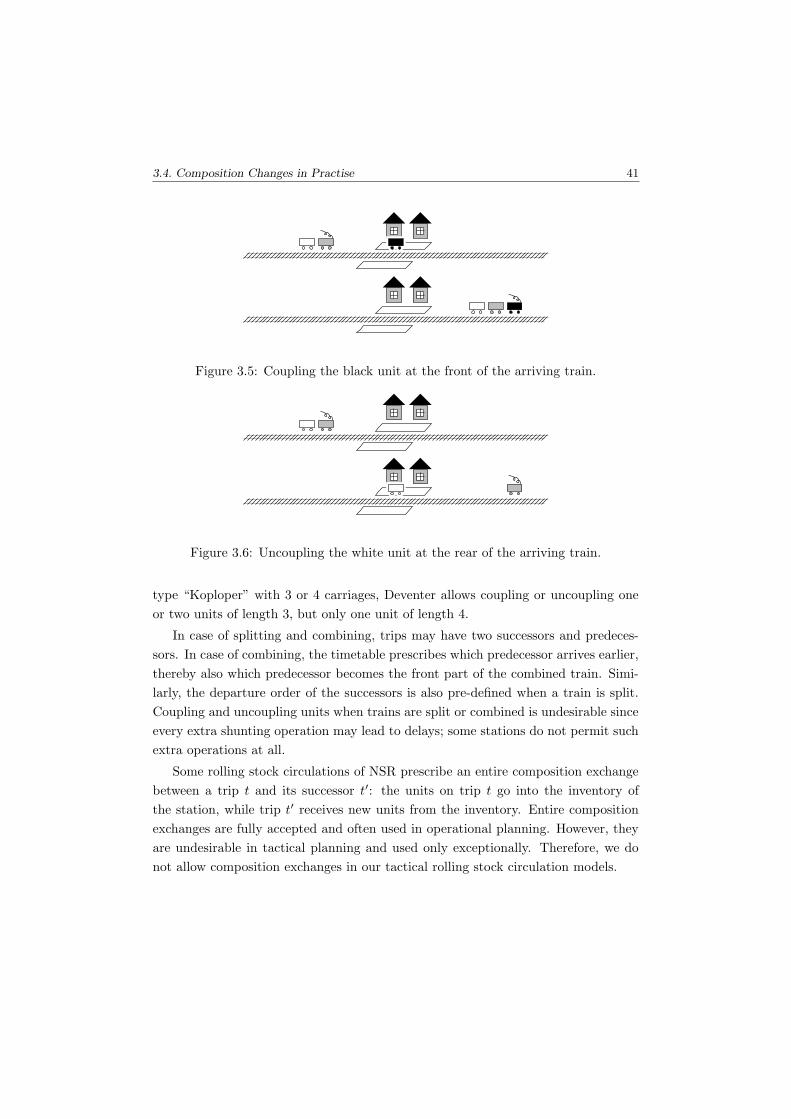
3.4. Composition Changes in Practise 41
Figure 3.5: Coupling the black unit at the front of the arriving train.
Figure 3.6: Uncoupling the white unit at the rear of the arriving train.
type “Koploper” with 3 or 4 carriages, Deventer allows coupling or uncoupling one
or two units of length 3, but only one unit of length 4.
In case of splitting and combining, trips may have two successors and predeces-
sors. In case of combining, the timetable prescribes which predecessor arrives earlier,
thereby also which predecessor becomes the front part of the combined train. Simi-
larly, the departure order of the successors is also pre-defined when a train is split.
Coupling and uncoupling units when trains are split or combined is undesirable since
every extra shunting operation may lead to delays; some stations do not permit such
extra operations at all.
Some rolling stock circulations of NSR prescribe an entire composition exchange
between a trip t and its successor t′: the units on trip t go into the inventory of
the station, while trip t′ receives new units from the inventory. Entire composition
exchanges are fully accepted and often used in operational planning. However, they
are undesirable in tactical planning and used only exceptionally. Therefore, we do
not allow composition exchanges in our tactical rolling stock circulation models.

42 Chapter 3. Tactical Rolling Stock Circulations
3.5 Problem Formulation
Now we can formulate the tactical rolling stock circulation problem at NSR. The
input consists of the following elements.
• The number of available units per type as well as the wished initial and final
inventories of the stations. (Later in this section we also discuss slightly less
specified input.)
• The timetable that specifies the departure and arrival times of the trips as
well as their successor and predecessor trips. Trips may have zero, one or two
predecessors and successors. Empty trains where the rolling stock circulation
may choose from are also explicitly given in the timetable.
• Upper and lower bounds are given on the length of a composition on each trip.
The upper bounds are determined by the lengths of the platforms along the
trip. The lower bounds are set according to the passenger demand.
• The list of allowed composition changes between a trip and its successor. We
discussed details of the allowed composition changes in Section 3.4.
• The estimated numbers of first and second class passengers for each trip. We
explain in Section 3.7 how the passenger demand is computed.
The output contains the compositions assigned to the trips and the duties for the
units. Recall that a duty of a unit describes which trips that unit serves in, also
specifying the position of the unit in the composition. The output must satisfy the
following primary constraints.
• Each composition change between a trip and its successor complies with the
specifications.
• The initial and final inventories at the stations are equal to the wished inven-
tories.
• The compositions assigned to the trips obey the lower and upper bounds in the
problem specification.
• The value of the objective function (described in Section 3.6) is as small as
possible.

3.5. Problem Formulation 43
Example. Consider the rolling stock circulation problem in Fig-
ure 3.7. The figure shows the time-space diagram between stations
s1 and s2 as well as four trips: trips with numbers 101 and 105
from s1 to s2 and their successor trips with numbers 102 and 106
back to s1. The wished initial inventory of station s1 is 3, the initial
inventory of station s2 is 1. The wished final inventories are equal
to the wished initial inventories.
Then a possible rolling stock schedule is to assign two units to trip
101 and to uncouple one of these units at s2, to assign one unit to
trip 105 and to couple a unit to it before departing as trip 106. Such
a rolling stock schedule is desirable if the passenger demand of trips
101 and 106 is much higher than on trips 102 and 105. The paths
of the units through the time-space diagram are indicated by bold
lines in the figure. We omitted the time periods from these paths
when the units are part of the inventories of the stations.
The rolling stock schedule described above is in fact feasible because
the unit that was located at s2 at the beginning is available to be
coupled to the arrived trip 105. Observe that if the time difference
between the arrival of trip 101 and the departure of trip 106 is
greater than the re-allocation time, the shunting crew has a choice
which unit should be coupled to the arriving trip 105.
s1
s2
101
105102
106
time
Figure 3.7: Example of a rolling stock circulation.
Besides these primary constraints, the instances may have additional secondary
constraints like the following three restrictions.
1. The continuity requirement states that if a timetable service admits underway
composition changes (i.e. it is divided into several trips), at least one unit
should follow the complete route of that service. It assures that passengers can
travel along the entire route of the timetable service without changing seats
underway.

44 Chapter 3. Tactical Rolling Stock Circulations
2. Most instances prescribe the initial and final inventories explicitly. These are
specified such that stations can satisfy the storage demand of all line groups.
Sometimes, usually for line groups that are planned first, the initial and final
inventories can be chosen arbitrarily. In such cases, it may make sense not to
specify the inventories but to require that for each station and for each type,
the initial inventory equals the final inventory. We call such a circulation a
cyclic solution. A reason for using cyclic solutions is that the expected number
of passengers on Tuesdays, Wednesdays and Thursdays are similar and that
the tactical timetables on these days are identical. Therefore, repeating an ap-
propriate cyclic solution three times immediately yields a rolling stock schedule
for these three days.
3. Stations have limited storage capacity. Therefore the instances may have an
explicit upper bound on the number of units (or on their total physical length)
that can be stored at a station at the same time.
Throughout the whole chapter, we use the following notations. Let M be the set
of rolling stock types. For each m ∈ M, let nm denote the number of available units
of type m, cm the number of carriages in a unit of type m and `m its physical length
in metres. The set of service classes is denoted by C. In instances of NSR, there are
two classes: first and second class. A unit of type m has κm,c seats of class c.
The set of stations is denoted by S. The wished initial and final inventory of
type m at station s is denoted by i0s,m and i∞s,m. Let T be the set of trips. A trip t
is characterised by its departure station sd (t), arrival station sa (t), departure time
τd (t) and arrival time τa (t). The length of the trip in kilometres is given by the
parameter dt. Trip t must receive compositions with at least µmint and at most µmax
t
carriages in total. The passenger demand per service class is δt,c.
If trip t has one successor, let σ (t) denote the successor of trip t. The re-allocation
time after trip t is % (t). If trip t has two successors, then they are denoted by σ1 (t)
and σ2 (t). The set T0 denotes the set of trips that have no predecessor trips, while
T∞ denotes the set of trips without successor trips.
3.6 Objective Criteria
Creating an appropriate rolling stock circulation means finding a balance between
several objectives such as minimising the number of carriage-kilometres (efficiency),
the amount of seat shortages (service quality) and the number of composition changes
3.7. Passenger Demand 45
(robustness). The models described in this chapter allow to make such a trade-off.
The objectives are explained below in detail.
The operational cost of rolling stock depends on traction power, but also on main-
tenance: after a certain number of kilometres, each unit is directed to a maintenance
facility for preventive check-up. These two factors are approximately proportional to
the carriage-kilometres.
The input of the tactical rolling stock circulation problem contains the estimated
number of first and second class passengers for every trip. Good service quality
means, among others, that all passengers, in particular first class passengers, have
a seat during their journey. Outside rush hours, rolling stock capacity is usually
sufficient for this. But during peak hours there may be more passengers than seats.
Our measure for the seat shortages is the sum over all trips of the expected number of
passengers without a seat, multiplied by the length of the trip. We call this measure
seat-shortage kilometres.
Compositions can be modified at certain stations by coupling units to a trip or
by uncoupling units from it. Changing the composition of a trip requires a number
of shunting movements between the platform area and the shunting area of a station.
This may lead to disturbances of the train operations. Moreover, there is always the
risk that coupling of the units does not work properly, causing additional delays.
Thus a smaller number of composition changes may increase the robustness of
the railway system. Moreover, the shunting costs are also related to the crew: each
shunting movement requires a train driver. On the other hand, changing the compo-
sitions between two trips may allow to use the rolling stock more efficiently and also
to decrease seat shortages.
Note that the quality of the solutions can be measured by several other charac-
teristics. For example, the largest seat shortage on a trip should not be too high (e.g.
at most 20% of the passengers of a trip during rush hours). Seat shortages in the
first class can be penalised more heavily than in the second class. Another criterion
is to keep the number of composition changes during rush hours small. The objective
function and the constraints in the models below can easily be modified in order to
take these additional criteria into account.
3.7 Passenger Demand
In tactical rolling stock circulations, the estimated number of passengers per trip is
part of the input. Here, we discuss briefly how these numbers are obtained.
46 Chapter 3. Tactical Rolling Stock Circulations
Throughout the whole year, conductors report the number of first and second class
passengers of each trip. Moreover, NSR employs or hires people to count passengers
and to enquire them about their journey. These counts serve as basis for both
the origin-destination matrix in line planning (see Section 2.2.2) and the passenger
demand used in tactical planning.
For each trip in the one-week timetable, the mean and the standard deviation of
the observations are computed. The passenger demand is set to the mean plus the
standard deviation. Tactical rolling stock planners try to allocate at least that many
seats to each trip. Then assuming that the observations have a normal distribution,
the allocated seat capacity is sufficient with a probability of at least 85%. This
definition of the passenger demand has been used for many years at NSR. One must
bear in mind that the conductors’ counts are somewhat unreliable. Experience shows
that the reported counts tend to be significantly too high.
In our models, we implemented this as follows. Here we only consider one of
the service classes, for sake of simpler notations. Suppose that passenger counts
d1, . . . , dk were observed for trip t with relative frequencies π1, . . . , πk and that the
standard deviation is s. Suppose that c seats are allocated for the trip. Then the
seat shortage on trip t is
max
(k∑
i=1
πidi + s − c, 0
). (3.3)
However, there are other possible measures for the seat shortages. A natural candi-
date is the expected number of seat shortages:
k∑
i=1
πi · max (di − c, 0) (3.4)
and eventually imposing the constraint that with a probability of 85%, there is no
seat shortage:
∑
i:di6c
πi > 85%. (3.5)
Replacing the traditional seat shortage measure (3.3) by (3.4) and eventually by (3.5)
in the models may lead to rolling stock circulations with quite differently distributed
seat shortages among the trips. Since decision makers have no unanimous opinion
when comparing circulations with different seat shortage structures, the alternative
measures for seat shortages have not been accepted (yet).

3.8. The Composition Model 47
3.8 The Composition Model
In this section, we describe a model that fits to the specifications of NSR and that can
be solved in a couple of hours even for the largest instances of NSR (and in a couple
of minutes for most instances) by commercial integer programming software. First,
we reformulate the problem slightly and specify the input formally. Subsequently,
we describe the basic model for the case when no splitting and combining is allowed.
Then we extend this basic model to handle splitting and combining of trains. Finally,
we report our computational results. Note that further computational results for the
Composition Model are given in Sections 3.11.5 and 5.5 where alternative methods
for generating rolling stock circulations are compared to the Composition Model.
3.8.1 Observation About the Duties
The output of the rolling stock circulation problem contains the duties of the rolling
stock units. However, one does not need to compute the duties explicitly. The
assumptions on the shunting process allow one to reformulate the problem:
The rolling stock circulation problem amounts to determining the com-
position of each trip such that after the departure of a trip from a station,
the inventory of each rolling stock type is non-negative.
Indeed, the composition of a trip and of its successor(s) unambiguously determine
the number of coupled and uncoupled units per type. Whenever units are to be
coupled to a trip, the inventory of the given station can satisfy this demand because
the inventory is non-negative after the departure. Then the rolling stock duties
themselves can be specified by matching the units entering the inventory of a station
to the units of the same type leaving the inventory. In practise, the matching can be
created in a Last-In-First-Out manner or in any other way which is convenient for
the shunting crew.
3.8.2 Integer Programming Model
In the basic model, we do not allow splitting and combining of trains. We need some
more notations.
A composition of units is an ordered sequence of elements of M. Taking again the
example of units with 3 and 4 carriages, the strings ‘334’ and ‘343’ represent com-
positions containing two units of length 3 and one unit of length 4. When assigning
compositions to trips, we assume that the right-hand side of the string corresponds
to the front of the train. The number of units in composition p is denoted by |p|. Let
48 Chapter 3. Tactical Rolling Stock Circulations
ν(p)m denote the number of units of type m in composition p. For a composition p,
let ν(p) be a vector in ZM with entries ν(p)m for each rolling stock type m ∈ M.
The set of compositions that are allowed for trip t is denoted by Pt. Members of
the set Pt must comply with the lower bound µmint and with the upper bound µmax
t
required for the train length on trip t.
Let Gt denote the set of pairs of compositions (p, p′) such that p ∈ Pt, p′ ∈ Pσ(t)
and such that the composition change from p to p′ after trip t is allowed. Thus the
shunting possibilities are encoded in the sets Gt.
Whenever a composition may be changed between trip t and its successor σ (t),
we assume that the units may be uncoupled from t, while units can be coupled to
σ (t). Finally, we assume that for a trip without a predecessor (i.e. for t ∈ T0), all
units serving t must be coupled just before t. Similarly, for a trip without a successor
(i.e. for t ∈ T∞), all units must be uncoupled just after t. These assumptions comply
with Figures 3.3 and 3.4.
The main decision variables in the model are the following:
Xt,p ∈ {0, 1} whether composition p is used for trip t (Xt,p = 1) or not
(Xt,p = 0).
Zt,p,p′ ∈ {0, 1} whether trip t has composition p and trip σ (t) has compo-
sition p′ (Zt,p,p′ = 1) or not (Zt,p,p′ = 0).
The variable Nt,m denotes the number of units of type m that are used on trip
t. We also use the variables Ct,m and Ut,m: Ct,m for the number of units of type m
that are to be coupled to right before trip t and Ut,m for the number of units of type
m that are to be uncoupled right after trip t.
The variable It,m denotes the inventory of type m at station sd (t) immediately
after the departure of trip t. The variables I0s,m and I∞s,m denote the number of units
of type m stored at station s at the beginning and at the end of the day.
Now, the basic part of the Composition Model reads as follows.
Minimise F (N,X,N) (3.6)
subject to
∑
p∈Pt
Xt,p = 1 ∀t ∈ T (3.7)
3.8. The Composition Model 49
Xt,p =∑
p′∈Pσ(t) :
(p,p′)∈Gt
Zt,p,p′ ∀t ∈ T \ T∞, p ∈ Pt (3.8)
Xσ(t),p′ =∑
p∈Pt :(p,p′)∈Gt
Zt,p,p′ ∀t ∈ T \ T∞, p′ ∈ Pσ(t) (3.9)
Nt,m =∑
p∈Pt
ν(p)mXt,p ∀t ∈ T, m ∈ M (3.10)
Cσ(t),m =∑
(p,p′)∈Gt :ν(p′)m>ν(p)m
(ν(p′)m − ν(p)m
)· Zt,p,p′ ∀t ∈ T \ T∞, m ∈ M (3.11)
Ut,m =∑
(p,p′)∈Gt :ν(p)m>ν(p′)m
(ν(p)m − ν(p′)m
)· Zt,p,p′ ∀t ∈ T \ T∞, m ∈ M (3.12)
Ct,m = Nt,m ∀t ∈ T0, m ∈ M (3.13)
Ut,m = Nt,m ∀t ∈ T∞ m ∈ M (3.14)
It,m = I0sd(t),m −
∑
t′∈T : sd(t′)=sd(t),
τd(t′)6τd(t)
Ct′,m
+∑
t′∈T : sa(t′)=sd(t),
τa(t′)6τd(t)−%(t′)
Ut′,m ∀t ∈ T, m ∈ M (3.15)
I∞s,m = I0s,m −
∑
t∈T :sd(t)=s
Ct,m +∑
t∈T :sa(t)=s
Ut,m ∀s ∈ S, m ∈ M (3.16)
I0s,m = i0s,m ∀s ∈ S, m ∈ M (3.17)
I∞s,m = i∞s,m ∀s ∈ S, m ∈ M (3.18)
Xt,p ∈ {0, 1} ∀t ∈ T, p ∈ Pt (3.19)
Nt,m, Ct,m, Ut,m, It,m ∈ R+ ∀t ∈ T m ∈ M (3.20)
I0s,m, I∞s,m ∈ R+ ∀s ∈ S, m ∈ M (3.21)
Zt,p,p′ ∈ R+ ∀t ∈ T (p, p′) ∈ Gt (3.22)
We describe the objective function (3.6) in detail in Section 3.8.4. Constraints
(3.7) state that, for each trip, exactly one allowed composition is used. Constraints
(3.8) and (3.9) guarantee correct composition changes between consecutive trips.
Constraints (3.10) link the compositions of a certain trip to the numbers of units
50 Chapter 3. Tactical Rolling Stock Circulations
of each type used on this trip. Constraints (3.11) – (3.14) specify the numbers
of coupled and uncoupled units. Constraints (3.15) describe the inventory of the
stations: The value It,m is the number of units that are stored at the station at the
begin of the day increased and decreased by one for each unit that is uncoupled or
coupled until the departure time of trip t. Recall that uncoupled units increase the
inventory only after the re-allocation time has elapsed, while coupled units decrease
the inventory immediately. Constraints (3.16) set the variables for final inventories.
Constraints (3.17) – (3.18) make sure that the initial and final inventories comply
with the problem specifications. Finally, constraints (3.19) – (3.22) describe the
variable domains.
One easily verifies the following lemma.
Lemma 3.1. In any feasible solution of the model (3.6) – (3.22), the variables Ut,m,
Ct,m, It,m, I0s,m, I∞s,m and Zt,p,p′ are integral.
Proof. The variables I0s,m and I∞s,m have fixed integer values. Then the binary vari-
ables Xp,m uniquely determine the value of Ut,m, Ct,m, It,m and Zt,p,p′ . �
Note that the composition changes could be modelled without the variables Zt,p,p′
but using additional linear constraints on the variables Xt,p:
Xσ(t),p′ 6∑
p∈Pt :(p,p′)∈Gt
Xt,p′ ∀t ∈ T \ T∞, p′ ∈ Pσ(t).
That is, a composition p′ can be assigned to trip σ (t) only if trip t has a composition p
that may go over to p′. Such a model is described by Alfieri et al. (2002). However, the
projection of the linear relaxation of their model onto the space of the variables Xt,p
strictly contains the projection of the linear relaxation of the Composition Model onto
the variables Xt,p. When applying a branch-and-bound procedure, the Composition
Model works with better lower bounds. Moreover, according to Lemma 3.1, one never
has to branch on a variable Zt,p,p′ . Thus we can expect that the number of nodes in
the branch-and-bound tree becomes smaller. On the other hand, the Composition
Model has to solve larger linear programs. State-of-the-art software such as CPLEX,
however, can cope with the linear programs that appear in our applications.
Observe that the model (3.6) – (3.22) can be interpreted as a single-commodity
network flow problem with side constraints. Indeed, consider the transition graph
defined on the node set
{(t, p) | t ∈ T, p ∈ Pt}
3.8. The Composition Model 51
and with arc set
{((t, p), (σ (t) , p′)
) ∣∣∣ t ∈ T \ T0, (p, p′) ∈ Gt
}.
Then the core of the model is formed by constraints (3.8) – (3.9), describing a network
flow problem in the transition graph. As we shall see soon, the objective function is
linear for this network flow problem.
3.8.3 Adding Secondary Constraints
The model (3.6) – (3.22) implements all primary constraints of the problem formu-
lation. Secondary constraints can be added to the model as follows.
Cyclic rolling stock circulations can be formulated by replacing the constraints
(3.17) and (3.18) by the following
nm =∑
s∈S
I0s,m ∀m ∈ M, (3.23)
I0s,m = I∞s,m ∀s ∈ S, m ∈ M. (3.24)
That is, for each type, the initial inventories add up to the number of available
units and the initial inventories are equal to the final inventories. According to the
following lemma, the variables I0s,m, I∞s,m and It,m may still be defined as continuous.
Lemma 3.2. Consider the model (3.6) – (3.16), (3.19) – (3.22), (3.23), (3.24) for
the problem of finding cyclic rolling stock circulations and suppose that the model has
a feasible solution. Then it has an integral optimal solution.
Proof. Consider an optimal solution and suppose that I0s1,m is not integral in this
solution for a station s1 and a type m. Then the variable I∞s1,m as well as of the
variables It,m with sd (t) = s1 have the same fractional part as I0s1,m has. Moreover,
(3.23) implies that I0s2,m is not integral for another station s2 as well. Again, the
variable I∞s2,m as well as the variables It,m with sd (t) = s2 have the same fractional
part as I0s2,m. Let ε = min{I0
s1,m; 1− I0s2,m}. Decreasing the variables I0
s1,m, I∞s1,m as
well as the variables It,m with sd (t) = s1 by ε and at the same time increasing the
variables I0s2,m, I∞s2,m as well as the variables It,m with sd (t) = s2 by ε and keeping
all other variables unchanged yields another feasible solution of the model. It is still
optimal since the objective function (3.6) only depends on the variables Nt,m, Xt,p
and Zt,p,p′ . Moreover, the number of variables with an integer value has increased.
Repeating this rounding step, one obtains an integral optimal solution. �

52 Chapter 3. Tactical Rolling Stock Circulations
The total physical length of the units stored at the stations at any moment is
expressed by the variables I0s,m, I∞s,m and It,m. Limitation on the storage capacity of
stations can be taken into account by the constraints
∑
m∈M
`m · It,m 6 Ws ∀ t ∈ T : sd (t) = s (3.25)
and by similar constraints for I0s,m and I∞s,m where `m is the length of a unit of type
m and Ws is the total storage capacity of station s. Note that the variables I0s,m
must be integral if constraints (3.25) are inserted into the model. Indeed, otherwise
two stations with storage capacity of 10 metres each could “share” a unit of length
20 metres. Once the variables I0s,m are integral, the integrality of the variables I∞
s,m
and It,m follows automatically.
For the continuity requirement, we need additional notations. Suppose that a
timetable service consists of trips t1, . . . , tk where ti+1 = σ (ti) for each i = 1, . . . , k−1
(see Figure 3.8). The continuity requirement states that at least one unit should serve
in each of the trips t1, . . . , tk. Without loss of generality we may assume that the
train carries out these trips without changing the riding direction. At the stations
underway, units may be coupled or uncoupled at the left- or the right-hand side of the
train. We index the units in a composition increasingly from the left: the left-most
unit has index 1, the second unit from the left has index 2, and so on.
︸ ︷︷ ︸t1
︸ ︷︷ ︸t2 . . .
︸ ︷︷ ︸tk
Figure 3.8: A timetable service composed of trips t1, . . . , tk.
For i = 1, . . . , k − 1, let αRi (and βR
i ) denote the total number of units (irrespec-
tive of their types) that are uncoupled from (coupled to) the right-hand side of the
composition after trip ti. Similarly, let αLi (and βL
i ) denote the number of uncoupled
(coupled) units on the left-hand side of the composition after trip ti. Let γi be the
number of units that serve on trip ti. Clearly, γi = γi−1 −αLi−1 −αR
i−1 + βLi−1 + βR
i−1
for every i = 2, . . . , k. These parameters are uniquely determined by the variables
Xt,p.
Suppose that a particular unit serves in trips t1, . . . , tk, let `i be its index in the
composition on trip ti. Then the numbers `i satisfy the following inequalities:

3.8. The Composition Model 53
`i ∈ Z ∀i = 1, . . . , k, (3.26)
1 6 `i 6 γi ∀i = 1, . . . , k, (3.27)
`i = `i−1 − αLi−1 + βL
i−1 ∀i = 2, . . . , k, (3.28)
`i 6 γi − αRi ∀i = 1, . . . , k − 1. (3.29)
Indeed, `i is an integer between 1 and γi. The indices `1, . . . , `k directly depend on
coupling and uncoupling at the left-hand side as described by (3.28). Finally, (3.29)
holds since the unit is not uncoupled after trip ti on the right-hand side.
Conversely, suppose that the system (3.26) – (3.29) with variables `1, . . . , `k has
a solution. Then the unit of index `1 on trip t1 serves in trips t2, . . . , tk with indices
`2, . . . , `k. That is, the continuity constraint is equivalent with the feasibility of the
system (3.26) – (3.29).
The values `i are determined by `1. Therefore (3.26) – (3.29) can be reformulated
as follows.
`1 ∈ R (3.30)
1 6 `1 6 γ1 (3.31)
1 6 `1 −∑
j<i
αLj +
∑
j<i
βLj 6 γi − αR
i ∀i = 2, . . . , k − 1 (3.32)
1 6 `1 −∑
j<k
αLj +
∑
j<k
βLj 6 γk (3.33)
The variables `2, . . . , `k are expressed in terms of `1. Moreover, there are only integral
lower and upper bounds on `1. Therefore `1 may be chosen continuous.
3.8.4 Objective Function
As was mentioned before, the objective function contains three major elements: (i)
carriage-kilometres, (ii) seat-shortage kilometres and (iii) the number of composition
changes. Given the above defined decision variables, these elements can be computed
easily.
For the total number of carriage-kilometres CKM, the following holds:
CKM(N) =∑
t∈T
∑
m∈M
dt · cm · Nt,m

54 Chapter 3. Tactical Rolling Stock Circulations
where dt is the length of trip t and cm is the number of carriages in a unit of type m.
The total number of seat-shortage kilometres SKM satisfies
SKM(X) =∑
c∈C
∑
t∈T
∑
p∈Pt
dt · st,p,c · Xt,p.
Here C is the set of service classes and st,p,c denotes the anticipated number of seat
shortages of class c when composition p is used for trip t. The shortage is computed
by comparing the forecasted number of passengers to the capacity of the compositions
as described in Section 3.7.
As stated in (3.1), coupling and uncoupling at the same time is not allowed.
Therefore, the total number of composition changes CCH can be determined by
adding all the variables Zt,p,p′ with ν(p) 6= ν(p′). Thus
CCH(Z) =∑
t∈T
∑
(p,p′)∈Gt :ν(p)6=ν(p′)
Zt,p,p′ .
The objective function F (X,Z,N) is a non-negative linear combination of these
criteria, the weight factors reflecting the relative importance. In order to control
the elements of the objective function more explicitly, we may also introduce upper
bounds on CKM, SKM and CCH.
3.8.5 New Integer Decision Variables
The variables Xt,p describe the exact composition for each trip t. Now it turns
out that, if new binary decision variables are introduced to describe the length of a
train, then the integrality constraint for the variables Xt,p can be dropped. By this
reformulation, the number of binary decision variables decreases. For example, in
the Noord-Oost instance, about 9,900 binary variables Xt,p are replaced by about
5,700 new binary variables.
The new decision variables determine the number of units per type that is allo-
cated to the trips, without specifying the exact order in the train. For a trip t, we
define the set of vectors in ZM+
Bt = {ν(p) | p ∈ Pt}.
Recall that ν(p) describes the numbers of units per type in composition p. We
introduce the binary variables

3.8. The Composition Model 55
Yt,b ∈ {0, 1} whether combination b ∈ Bt is used for trip t (Yt,b = 1) or
not (Yt,b = 0).
Their connection with the already defined variables Xt,p is described by
Yt,b =∑
p∈Pt : b=ν(p)
Xt,p ∀t ∈ T b ∈ Bt. (3.34)
The variables Yt,b correspond to the higher-level decisions like capacity allocation,
while the variables Xt,p fill in the fine details of the solution.
Theorem 3.3. Consider the model (3.6) – (3.22) extended by the binary variables
Yt,b and by the constraints (3.34). Replace the constraint (3.19) in this model by
0 6 Xt,p 6 1 ∀t ∈ T and p ∈ Pt. Then this relaxed mixed integer program has an
integral optimal solution whenever it has a feasible solution.
Proof. Let (X,Y,N,C,U, I0, I∞, I, Z) be an optimal solution of the relaxed problem:
the variables Yt,b are binary, while the variables Xt,p may have fractional values.
Consider the transition graph defined in Section 3.8.2. Set the capacity of an arc to
0 if the corresponding value Zt,p,p′ is zero and set the capacity to 1 otherwise. The
values Zt,p,p′ form a network flow in this graph. Thus there exists an integer valued
network flow Zt,p,p′ with the same amount of flow. Define the values Xt,p according
to the constraints (3.8) – (3.9).
We shall prove that if we fix the binary values of the variables Yt,b in the relaxed
model, then the values of the variables Nt,m, Ct,m, Ut,m, I0s,m, I∞s,m and It,m as
well as the objective criteria CKM, SKM and CCH are uniquely determined even
if Xt,p and Zt,p,p′ may have fractional values. Then it follows immediately that
(X, Y,N,C, U, I0, I∞,I, Z) is an integral feasible (and optimal) solution of the relaxed
model.
Indeed, the value of the variables I0t,m and I∞t,m is fixed by the constraints. More-
over, one easily derives that for each trip t and rolling stock type m, we have
Nt,m =∑
b∈Bt
bmYt,b. (3.35)
Consider now any trip t. The integrality of the variables Yt,b implies that a variable
Xt,p can have a positive value only if the composition p contains as many units of
each type as the variables Nt,m indicate. Then (3.8) and (3.9) imply that all members
of the set
{(p, p′) ∈ Gt | Zt,p,p′ > 0}

56 Chapter 3. Tactical Rolling Stock Circulations
have the same differences ν(p′)m − ν(p)m for every m ∈ M (namely Nσ(t),m −Nt,m).
Therefore
Ct,m = max{Nσ(t),m − Nt,m, 0
}
and
Ut,m = max{Nt,m − Nσ(t),m, 0
}.
Then it follows that the variables It,m are also uniquely determined.
Clearly, the number of carriage-kilometres CKM only depends on the variables
Yt,b. Moreover, the number of seat-shortage kilometres SKM is also determined by
the variables Yt,b. Indeed, all compositions that correspond to a certain combination
b ∈ Bt have the same capacity and thus the same amount of seat shortages (denoted
by st,b) on trip t. Therefore
SKM =∑
t∈T
∑
b∈Bt
dt · st,b · Yt,b.
Finally, each trip has a contribution
∑
ν(p)6=ν(p′)
Zt,p,p′
to the number of composition changes CCH. This contribution is 1 if Nt,m 6= Nσ(t),m
for some rolling stock type m and 0 otherwise. Then (3.35) implies that CCH is
determined by the variables Yt,m. �
3.8.6 Splitting and Combining Trains
In order to handle splitting and combining trains, we use an extension of the basic
model. First, we describe splitting trains.
Let Ts be the set of trips after which the corresponding train is split into two
trains. Then for each trip t ∈ Ts, there are two trips σ1 (t) and σ2 (t) that take place
immediately after splitting trip t. Recall that the departure order of the trips σ1 (t)
and σ2 (t) is determined by the timetable.
Let Gst be the set of 3-tuples (p, p1, p2) such that p ∈ Pt, p1 ∈ Pσ1(t), p2 ∈ Pσ2(t)
and p is the concatenation of the strings p1 and p2. We introduce a variable
Zst,p,p1,p2
∈ [0, 1] (3.36)

3.8. The Composition Model 57
for each t ∈ Ts and (p, p1, p2) ∈ Gst . These variables are linked to the other variables
similarly to the constraints (3.8) – (3.9):
Xt,p =∑
p1,p2 : (p,p1,p2)∈Gst
Zst,p,p1,p2
∀p ∈ Pt, (3.37)
Xσ1(t),p1=
∑
p,p2 : (p,p1,p2)∈Gst
Zst,p,p1,p2
∀p1 ∈ Pσ1(t), (3.38)
Xσ2(t),p2=
∑
p,p1 : (p,p1,p2)∈Gst
Zst,p,p1,p2
∀p2 ∈ Pσ2(t). (3.39)
It may be possible to modify the compositions further by allowing to couple or
uncouple units when the train is split. This can easily be modelled by modifying the
sets Gst . The variables Ct,m and Ut,m as well as the objective function should then
also be adjusted as follows. Assuming that units may be uncoupled from the arriving
trip t ∈ Ts and may only be coupled to σ1 (t), the following constraints are needed
for each m ∈ M:
Ut,m =∑
(p,p1,p2)∈Gst :
ν(p1)m+ν(p2)m>ν(p)m
(ν(p1)m + ν(p2)m − ν(p)m
)· Zs
t,p,p1,p2, (3.40)
Cσ1(t),m =∑
(p,p1,p2)∈Gst :
ν(p)m>ν(p1)m+ν(p2)m
(ν(p)m − ν(p1)m − ν(p2)m
)· Zs
t,p,p1,p2, (3.41)
Cσ2(t),m = 0. (3.42)
Furthermore, the objective function must be adjusted by adding the following
term to the number of composition changes:
∑
t∈Ts
∑
(p,p1,p2)∈Gst :
ν(p)6=ν(p1)+ν(p2)
Zst,p,p1,p2
.
Combining two trains can be described in a similar way. One defines the set Tc
of trips t that have two predecessors t1, t2 as well as the sets Gct of 3-tuples (p, p1, p2)
such that p ∈ P(t), p1 ∈ P(t1), p2 ∈ P(t2) and p is the concatenation of the strings
p1 and p2. Then one introduces the variables Zct,p,p1,p2
for t ∈ Tc and (p, p1, p2) ∈ Gct .
Then Lemma 3.1 extends to the following lemma.

58 Chapter 3. Tactical Rolling Stock Circulations
t1
t2
t3
t4
t5 t6
splitting combining
3434
4343
34
43
34
43
34
43
34
43
3434
4343
Figure 3.9: A pair of splitting and combining events and the corresponding compo-sition graph. The composition is reversed after trip t3.
Lemma 3.4. In any feasible solution of the model (3.6) – (3.22), (3.36) – (3.39)
and eventually (3.40) – (3.42), the variables Ut,m, Ct,m, I0s,m, I∞s,m, It,m, Zt,p,p′ and
Zst,p,p1,p2
have integral values.
Also in the case of splitting and combining we can introduce the decision variables
Yt,b described in Section 3.8.5. Unfortunately, Theorem 3.3 does not extend. The
following example shows that introducing the variables Yt,b and relaxing the variables
Xt,p may lead to a feasible model which does not have any feasible integral solution.
Example. Figure 3.9 indicates trips t1, . . . , t6. Trip t1 is split into
trips t2 and t3. The successors of t2 and t3 are t4 and t5, they are
combined to trip t6. The composition is unchanged after trip t2 but
reversed after trip t3.
Trips t1 and t6 can have composition ‘3434’ or ‘4343’ and trips
t2, t3, t4, t5 can have composition ‘34’ or ‘43’. Then we have
Pt1 = Pt6 = {3434, 4343}, Pt2 = Pt3 = Pt4 = Pt5 = {34, 43},
Gst1 = {(3434, 34, 34), (4343, 43, 43)}, Gt2 = {(34, 34), (43, 43)},
Gt3 = {(34, 43), (43, 34)} and Gct6 = {(3434, 34, 34), (4343, 43, 43)}.
Setting the variables Xti,p with i = 1, . . . , 6 and p ∈ Ptito 1
2 and
setting also all variables Z,Zs and Zc to 12 yields a fractional so-
lution of the Composition Model. There is, however, no integral
solution.
So we required all variables Yt,b and Xt,p to be integral. However, when we
tested the model with Xt,p relaxed to rational, we always found fully integral optimal
solutions. Therefore we gave the variables Yt,b higher priority than the variables Xt,p
(see Section 3.10.1).
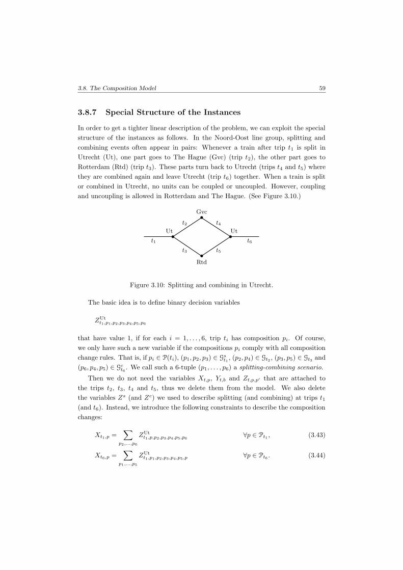
3.8. The Composition Model 59
3.8.7 Special Structure of the Instances
In order to get a tighter linear description of the problem, we can exploit the special
structure of the instances as follows. In the Noord-Oost line group, splitting and
combining events often appear in pairs: Whenever a train after trip t1 is split in
Utrecht (Ut), one part goes to The Hague (Gvc) (trip t2), the other part goes to
Rotterdam (Rtd) (trip t3). These parts turn back to Utrecht (trips t4 and t5) where
they are combined again and leave Utrecht (trip t6) together. When a train is split
or combined in Utrecht, no units can be coupled or uncoupled. However, coupling
and uncoupling is allowed in Rotterdam and The Hague. (See Figure 3.10.)
Ut Ut
Gvc
Rtd
t1 t6
t2
t3
t4
t5
Figure 3.10: Splitting and combining in Utrecht.
The basic idea is to define binary decision variables
ZUtt1,p1,p2,p3,p4,p5,p6
that have value 1, if for each i = 1, . . . , 6, trip ti has composition pi. Of course,
we only have such a new variable if the compositions pi comply with all composition
change rules. That is, if pi ∈ P(ti), (p1, p2, p3) ∈ Gst1 , (p2, p4) ∈ Gt2 , (p3, p5) ∈ Gt3 and
(p6, p4, p5) ∈ Gct6 . We call such a 6-tuple (p1, . . . , p6) a splitting-combining scenario.
Then we do not need the variables Xt,p, Yt,b and Zt,p,p′ that are attached to
the trips t2, t3, t4 and t5, thus we delete them from the model. We also delete
the variables Zs (and Zc) we used to describe splitting (and combining) at trips t1
(and t6). Instead, we introduce the following constraints to describe the composition
changes:
Xt1,p =∑
p2,...,p6
ZUtt1,p,p2,p3,p4,p5,p6
∀p ∈ Pt1 , (3.43)
Xt6,p =∑
p1,...,p5
ZUtt1,p1,p2,p3,p4,p5,p ∀p ∈ Pt6 . (3.44)

60 Chapter 3. Tactical Rolling Stock Circulations
These are analogous with constraints (3.8) – (3.9) and (3.37) – (3.39).
We still need the variables Iti,m for i = 1, . . . , 6 to ensure non-negative inventories
at any moment. Moreover, in order to keep track of the number of (un)coupled units
in Rotterdam and The Hague, we use integer variables Ut2,m, Ut3,m, Ct4,m and Ct5,m
and express them as weighted sums of the variables ZUt as follows.
Ut1,m = Ct2,m = Ct3,m = 0 ∀m ∈ M (3.45)
Ut4,m = Ut5,m = Ct6,m = 0 ∀m ∈ M (3.46)
Ut2,m =∑
p1,...,p6 :ν(p2)m>ν(p4)m
(ν(p2)m − ν(p4)m
)· ZUt
t1,p1,p2,p3,p4,p5,p6∀m ∈ M (3.47)
Ct4,m =∑
p1,...,p6 :ν(p4)m>ν(p2)m
(ν(p4)m − ν(p2)m
)· ZUt
t1,p1,p2,p3,p4,p5,p6∀m ∈ M (3.48)
Ut3,m =∑
p1,...,p6 :ν(p3)m>ν(p5)m
(ν(p3)m − ν(p5)m
)· ZUt
t1,p1,p2,p3,p4,p5,p6∀m ∈ M (3.49)
Ct5,m =∑
p1,...,p6 :ν(p5)m>ν(p3)m
(ν(p5)m − ν(p3)m
)· ZUt
t1,p1,p2,p3,p4,p5,p6∀m ∈ M (3.50)
The variables ZUt appear in the objective function with weights that indicate the
carriage-kilometres, seat-shortage kilometres and the number of composition changes
for the deleted trips t2, . . . , t5. It follows immediately that the model modified in such
a way still describes the same rolling stock circulation problem. One might wonder
whether the integrality of the variables ZUt can always be relaxed. Unfortunately,
this cannot always the case as the following example shows.
Example. Suppose that penalties for composition changes are the
only non-zero weighted terms in the objective function. Suppose
that trip t1 has composition ‘3333’ (i.e. 4 units with 3 carriages) and
trip t6 has composition ‘33’. Moreover, suppose that the other parts
of the model enforce uncoupling one unit each both at The Hague
and at Rotterdam, that is Ut2,3 = Ut3,3 = 1. Then there is only
one splitting-combining scenario that realises these requirements:
assigning composition ‘33’ to both t2 and t3 and uncoupling one
unit each at both The Hague and Rotterdam (see Figure 3.11(a)).
This solution pays twice the composition change penalty.

3.8. The Composition Model 61
However, there is a cheaper fractional solution: We have a vari-
able ZUt1 (with somewhat sloppy notation) of a splitting-combining
scenario which assigns composition ‘333’ to trip t2 and composi-
tion ‘3’ to t3, t4 and t5 (see Figure 3.11(b)). Moreover, we have a
variable ZUt2 of another splitting-combining scenario which assigns
composition ‘333’ to trip t3 and composition ‘3’ to t2, t4 and t5
(see Figure 3.11(c)). These latter solutions pay the penalty for the
composition changes only once, but they do not comply with the
external inventory restrictions. However, the solution 12ZUt
1 + 12ZUt
2
does and it pays the composition change penalty only once.
(a)
Ut Ut
Gvc
Rtd
t1 t6
t2
t3
t4
t5
‘3333’ ‘33’
‘33’
‘3’
‘3’
‘33’
(b)
Ut Ut
Gvc
Rtd
t1 t6
t2
t3
t4
t5
‘3333’ ‘333’
‘3’
‘3’
‘3’
‘33’
(c)
Ut Ut
Gvc
Rtd
t1 t6
t2
t3
t4
t5
‘3333’ ‘3’
‘333’
‘3’
‘3’
‘33’
Figure 3.11: Three different ways of splitting and combining in Utrecht.
The following example shows that integer solutions may not exist even if the
linear relaxation of the problem has a feasible solution.
Example. Consider the two splitting-combining scenarios in Fig-
ure 3.12(a) and Figure 3.12(b). They both give feasible ways to
obtain a composition ‘3443’ on trip t6 from a composition ‘3333’ on
trip t1. However, taking the convex combination of the correspond-
ing variables ZUt with coefficients 12 would describe a composition
change shown in Figure 3.12(c): uncoupling a unit of length 3 and
coupling a unit of length 4 at the same time both in The Hague and
in Rotterdam. This is not allowed in our shunting model.
In order to avoid such troubles when relaxing the integrality of the variables ZUt,
we introduce the binary variables UGvc and URtd that express whether or not units

62 Chapter 3. Tactical Rolling Stock Circulations
(a)
Ut Ut
Gvc
Rtd
t1 t6
t2
t3
t4
t5
‘3333’ ‘333’
‘3’
‘3’
‘443’
‘3443’
(b)
Ut Ut
Gvc
Rtd
t1 t6
t2
t3
t4
t5
‘3333’ ‘3’
‘333’
‘344’
‘3’
‘3443’
(c)
Ut Ut
Gvc
Rtd
t1 t6
t2
t3
t4
t5
‘3333’ ‘33’
‘33’
‘34’
‘43’
‘3443’
Figure 3.12: Two legal splitting-combining scenarios (a) and (b) and an impossibleone (c).
are uncoupled after the arrival of trip t2 and t3. Similarly, we introduce the binary
variables CGvc and CRtd that express whether or not units are coupled before the
departure of trips t4 and t5. These variables can also be written as sums of the
variables ZUt:
UGvc =∑
p1,...,p6 : |p2|>|p4|
ZUtt1,p1,p2,p3,p4,p5,p6
, (3.51)
URtd =∑
p1,...,p6 : |p3|>|p5|
ZUtt1,p1,p2,p3,p4,p5,p6
, (3.52)
CGvc =∑
p1,...,p6 : |p4|>|p2|
ZUtt1,p1,p2,p3,p4,p5,p6
, (3.53)
CRtd =∑
p1,...,p6 : |p5|>|p3|
ZUtt1,p1,p2,p3,p4,p5,p6
. (3.54)
The following lemma states that these additional variables in fact suffice to relax
the integrality of the variables ZUt. The proof uses the following specific properties
of the Noord-Oost line group:
• There are two rolling stock types: units with 3 carriages and units with 4
carriages.
• Each trip has at most 15 carriages.

3.8. The Composition Model 63
• At most two units can be coupled or uncoupled at the same time.
• Every time when a train is split in Utrecht, its left-most part continues to The
Hague and its right-most part continues to Rotterdam. Similarly, every time
when trains are combined in Utrecht, the left-most part arrives from The Hague
and the right-most part arrives from Rotterdam.
These properties may or may not hold for other instances.
Lemma 3.5. Consider the Composition Model and modify it for a single pair of
splitting-combining events as described above. That is, delete the variables X, Y , Z,
Zs and Zc that are attached to the trips t2, . . . , t5. Moreover, require Cti,m and Uti,m
to be integral for i = 2, . . . , 5 and for each m ∈ M. Introduce the binary variables
CGvc, CRtd, UGvc and URtd, as well as continuous variables ZUt in the range [0; 1].
Finally, add the constraints (3.43) – (3.54) to the model. Then this model has an
integral optimal solution whenever it has a feasible solution.
Proof. Consider an optimal solution of the model. We claim that for each splitting-
combining scenario (p1, . . . , p6) with ZUtt1,p1,p2,p3,p4,p5,p6
> 0 and for each m ∈ M, we
have
Ut2,m = max {ν(p2)m − ν(p4)m, 0} .
That is, in each splitting-combining scenario that has positive value in the solution,
Ut2,m units of type m are uncoupled at The Hague after trip t2.
Indeed, if UGvc = 0, then the claim follows from (3.47) and (3.51). Suppose now
that UGvc = 1. Then each splitting-combining scenario with positive ZUt value un-
couples either one or two units in The Hague after trip t2. For each rolling stock type,
zero, one or two units are uncoupled in any splitting-combining scenario. Equation
(3.47) can be interpreted as the weighted sum of the positive variables ZUt where
the weights ν(p2)m − ν(p4)m are either zero or one or two:
Ut2,m =∑
p1,...,p6 : |p2|>|p4| and
ZUtt1,p1,p2,p3,p4,p5,p6
>0
(ν(p2)m − ν(p4)m
)· ZUt
t1,p1,p2,p3,p4,p5,p6. (3.55)
If no weight zero or two appears in (3.55), then all weights must be equal – just as we
claimed – since Ut2,m is an integer number. Thus we may assume that both weights
zero and two occur in (3.55).

64 Chapter 3. Tactical Rolling Stock Circulations
Let m′ denote the other rolling stock type. Then the number of uncoupled units
per type can be as follows:
m m′ Sum of ZUt values
2 0 α1
1 0 α2
1 1 α3
0 1 α4
0 2 α5
The numbers αi are the sums of the variables ZUt that correspond to the numbers
of uncoupled units per type. These numbers αi satisfy
α1, . . . , α5 > 0,
5∑
i=1
αi = 1.
We also have
α1 > 0,
α4 + α5 > 0
since these are the sums of the variables ZUt that have weight zero and two in (3.55),
respectively. Moreover,
Ut2,m = 2α1 + α2 + α3,
Ut2,m′ = 2α5 + α3 + α4.
Therefore, using the fact that Ut2,m and Ut2,m′ are equal to 0, 1 or 2, one easily
derives that
α1 = α5 > 0.
That is, there exists a splitting-combining scenario where two units of type m are
uncoupled in The Hague and there exists another splitting-combining scenario where
two units of type m′ are uncoupled. Therefore, the composition on trip t1 (which is
the same in every splitting-combining scenario with positive value ZUt) must contain
both of the substrings mm and m′m′. Using units with 3 or 4 carriages and having
3.9. Solution Approaches 65
an upper bound of 15 carriages on the train lengths, it means that the composition
used in trip t1 must be either mmm′m′ or m′m′mm.
Suppose that t1 has composition mmm′m′ (the other case being analogous). After
splitting, always the left-hand side of the split train goes to The Hague. Thus the
splitting-combining scenario which uncouples two units of type m′ requires that the
entire train of t1 goes to The Hague, not leaving any unit for trip t3. However, every
splitting-combining scenario allocates at least unit to each of the trips t2, . . . , t5.
One can show similarly that all splitting-combining scenarios with positive value
ZUt intend to uncouple Ut3,m units of type m at Rotterdam and to couple Ct4,m
and Ct5,m units of type m at The Hague and Rotterdam. That is, these splitting-
combining scenarios may be different but their connection to the rest of the model
is identical. Then an optimal solution uses only one of them: the one that has the
smallest coefficient in the objective function. �
3.9 Solution Approaches
Having developed the Composition Model for the rolling stock circulation problem,
we still have to solve it. In this section, we describe two solution approaches.
Peeters and Kroon (2003) describe the model above for line groups without split-
ting and combining. Their main idea is to focus on the network flow structure of the
problem. Being a single-commodity flow problem in the transition graph, the model
admits Dantzig-Wolfe decomposition for solving the linear relaxation quickly: define
a variable for each directed path in the graph and write the network flow as the sum
of the path flows. The paths in the transition graph only interact in the inventory
constraints. Once the linear relaxation is solved, a branch-and-price framework is ap-
plied to obtain integer solutions. This approach works very well when implemented
for real-life instances of NSR without splitting and combining. Within a couple of
seconds, the instances can be solved to optimality.
This solution method extends for splitting and combining only if after splitting
a train, the split parts are combined with each other again as shown in Figure 3.10.
However, about one third of the splitting-combining events in the Noord-Oost line
group behave differently. If a train is split in Amersfoort, the part going to Ams-
terdam will not meet again the other going to Schiphol. Both parts do turn back,
but the part arriving back from Schiphol can only catch a train from Amsterdam
that was split in Amersfoort an hour later (see Figure 3.13). This property of the
timetable makes the appealing Dantzig-Wolfe decomposition approach impossible.

66 Chapter 3. Tactical Rolling Stock Circulations
7:00 7:30 8:00 8:30 9:00 9:30 10:00
Amf
Asd
Shl
Figure 3.13: Trains between Amersfoort (Amf), Amsterdam (Asd) and Schiphol(Shl). After splitting in Amersfoort, the two parts do not meet any more.
Focusing from the beginning on the Noord-Oost problem, in this thesis we use
a commercial MIP solver to obtain solutions. In order to obtain solutions quickly,
various techniques need to be applied. We discuss the computational results for the
Noord-Oost problem in the next section. Computational results for the Composition
Model on other instances of NSR are reported in Sections 3.11.5 and 5.5.
3.10 Computational Results for the Noord-Oost
For our computations, we use the modelling software ILOG OPL Studio 3.7 and the
mixed integer programming solver ILOG CPLEX 9.0 on a PC with an Intel Pentium
IV 3.0 GHz processor and with 512 Mb internal memory. Our goal is to find feasible
solutions of good quality in reasonable time. Mostly, we stop the computations after
a couple of hours of CPU time.
We implement the Composition Model for the Noord-Oost line group for a generic
Tuesday. Lacking specified initial and final inventories, we look for cyclic solutions.
We consider several problem instances with the same timetable, the instances differ
in explicit bounds on the objective criteria and in their weight factors in the objective
function.
We compare our solutions to a manually created rolling stock circulation. In
Table 3.1 we give the values of the three objective criteria in this reference solution.
Experiments are carried out with several objective functions. The weight factors
for carriage-kilometres (CKM), seat-shortage kilometres (SKM) and the number of
composition changes (CCH) are also given in Table 3.1. According to the preferences
of NSR, we give a low weight factor to CKM in the objective function but require

3.10. Computational Results for the Noord-Oost 67
CKM SKM CCHvalue in practise 317,853 555,215 135weight in Obj1 1 1 5,000weight in Obj2 1 1 1,000weight in Obj3 1 1 100weight in Obj4 1 10 1,000weight in Obj5 1 10 100
Table 3.1: The values of the objective criteria in the reference solution and the weightfactors used in the experiments.
Without aggregation With aggregationMIP Reduced MIP MIP Reduced MIP
# integer var. 16,992 – 15,848 –# contin. var. 33,901 – 44,769 –# variables 50,893 34,228 60,617 39,251# constraints 32,308 17,896 28,149 15,348# non-zeros 195,184 136,105 287,286 177,622
Table 3.2: Dimensions of the MIP’s: number of variables (integer and continuous),constraints and non-zeros in the matrix. Columns under ‘With aggregation’ areobtained by implementing the variables and constraints described in Section 3.8.7.
the constraint
CKM 6 318, 000 (3.56)
expressing that the number of carriage-kilometres is not higher than in the reference
solution. In additional experiments we explicitly minimise the carriage-kilometres
while giving bounds on seat-shortages and the number of composition changes.
The first two columns of Table 3.2 (under ’Without aggregation’) contain the
dimensions of the mixed integer program as well as the size of the reduced MIP,
created by CPLEX in the pre-processing phase.
Finding feasible solutions of good quality turns out to be quite time-consuming.
In order to speed up the solution process, we apply various techniques.
3.10.1 CPLEX Parameters
Fine-tuning the parameters of CPLEX has a large impact on the solution times. We
use the barrier method to solve the root node of the branch-and-bound tree. Then

68 Chapter 3. Tactical Rolling Stock Circulations
we apply the dual simplex method for any other node. Using the built-in heuristics
frequently, applying probing, perturbing the objective function and using branching
priorities (explained below) turns out to be particularly helpful.
The variables have a hierarchical structure. The variables Nt,m describe the
number of units of a given type m used for trip t. The variables Yt,b represent
decisions one level lower, while the variables Xt,p specify the finer details. As we
observed, the objective criteria are basically functions of the variables Yt,b.
It turns out to be advantageous to branch first on the variables Nt,m, then on the
variables Yt,b and at last on the variables Xt,p. This can be explained as follows. The
values Nt,m describe a rough estimate of the solution. Nevertheless, early decisions
on train lengths determine a large part of the objective function. Therefore, the
branch-and-bound process can work out the exact compositions subject to good lower
bounds. We mentioned in Section 3.8.6 that, once the variables Yt,b are integral, the
variables Xt,p are likely integral, too. So, our branching order often has the effect
that we did not need to branch on the variables Xt,p at all.
Giving a higher branching priority to the decision variables corresponding to trips
in the rush hours also leads to an improvement of the solution time. Seat shortages
mostly occur in such trips, thus very good lower bounds on the seat shortages can be
computed in the early stage of the algorithm. Then the rolling stock assignment for
the rush hours extends to the rest of the day, providing good suboptimal solutions
relatively quickly.
3.10.2 Exploiting the Structure of the Instances
When applying the aggregation described in Section 3.8.7, the mixed integer program
contains more variables but less constraints. The dimensions of the mixed integer
program are given in the two last columns of Table 3.2 (under ‘With aggregation’).
The LP relaxation with aggregation provides slightly better bounds than in the
case of no aggregation. Although the difference is small, about 0.1–0.9% of the
optimal objective value, even this improvement results in speeding up the solution
process. The effect of using the aggregation is presented in Table 3.3. In three test
instances, we impose the constraint (3.56) and different bounds (if any) on CCH. We
test all instances with and without aggregation, minimising the 5 objective functions
in Table 3.1. In each row, we give the optimality gap proved in 2 hours of computation
and after how many seconds the best solution was found. A field without numbers
means that no feasible solution was found within 2 hours. We can see that the
aggregation significantly improves the performance of the branch-and-bound process.

3.10. Computational Results for the Noord-Oost 69
CKM CCH Aggr Obj1 Obj2 Obj3 Obj4 Obj5318,000 – Yes 1.69% 0.22% opt opt opt
3,000 3,200 2,000 1,900 2,700318,000 – No 2.56% 0.76% opt 0.12% opt
5,400 5,000 5,000 4,300 4,400318,000 120 Yes 2.30% 0.50% 1.24% 2.22% 2.32%
3,500 7,100 3,400 6,500 5,100318,000 120 No 2.06% 0.67% — 11.20% 13.16%
4,800 6,400 — 6,300 5,000318,000 90 Yes 4.80% 2.67% — 11.43% —
6,000 7,100 — 6,400 —318,000 90 No 4.90% 16.11% — — —
5,700 5,300 — — —
Table 3.3: For each test instance: i) optimality gap after 7200 seconds, ii) timeelapsed till the best solution was found (in seconds).
We analyse the performance of the model with aggregation in the following se-
quence of tests: We minimise the seat-shortage kilometres while using the bound of
318,000 on CKM and imposing every possible upper bound between 50 and 155 on
CCH. We allow 2 hours of CPU time for each instance. The computational results
are summarised in Figure 3.14. The x- and y-axis of the graph correspond to SKM
and CCH. The continuous curve indicates the linear programming lower bound, the
dashed curve shows the best lower bound obtained after 2 hours of computations.
The dots indicate the solutions themselves. It turns out that the linear program-
ming lower bound is hardly improved during the branch-and-bound procedure. We
can conclude that performance of the solution process highly depends on the upper
bound of CCH: with upper bounds of 115 or higher, almost optimal solutions can
be found, while upper bounds up to 95 hardly admit any feasible solutions within 2
hours.
3.10.3 Heuristic Approaches
Search Around the LP Optimum
For some instances, no feasible solution can be found in 2 hours of computation or
the quality of the solutions is not satisfactory. This is often the case if bounds on
the number of composition changes are too restrictive. Also minimising the carriage-
kilometres only while imposing upper bounds on seat-shortages and the number of

70 Chapter 3. Tactical Rolling Stock Circulations
300,000 400,000 500,000
50
100
150
CCH
SKM
reference solution
Figure 3.14: Minimising seat-shortage kilometres (SKM) with different bounds on thenumber of composition changes (CCH) and with at most 318,000 carriage-kilometres.
composition changes often hits the CPU-time limit of a couple of hours without
providing solutions with a small optimality gap.
Computational results in the previous section show that the difference between
the objective value of the linear relaxation and the best lower bound proved during
the branch-and-bound process is small, at most 2%. Moreover, solutions with a small
optimality gap indicate that the Composition Model is a quite tight description of
the convex hull of the integral solutions. This justifies the following heuristic method.
We first solve a relaxation of the problem, dropping the integrality requirements
for some variables (e.g. taking the linear relaxation itself). Then we extract informa-
tion from the optimal (fractional) solution of the relaxation and based on it, we add
extra constraints to the original model. In the simplest form, we require Xt,p = 0
whenever this variable has value zero in the optimal solution of the relaxed model.
As another example, we allow a composition change (that is, extra shunting) after
trip t only if the optimal solution of the relaxation has a variable Zt,p,p′ > 0 with
ν(p) 6= ν(p′).
Reducing the solution space in this way allows us to find feasible solutions within
2 hours for each instance. The optimality gap is, however, still over 10% in some
instances. Nevertheless, even these solutions are in all objective criteria better than
the reference solution from practise.

3.10. Computational Results for the Noord-Oost 71
When trying several ways to use optimal fractional solutions in order to guide
the MIP solution process, we experienced that the improvement in running time
strongly depends on the instances themselves. Therefore, we cannot conclude which
is the best way of using the relaxed solutions. Nonetheless, after a couple of attempts
and a couple of hours of CPU time, we almost always find good integer solutions.
Local Search
Once a feasible solution Σ was found, we can run the model in some “neighbourhood”
of this solution. We define the neighbourhood by constraints like saying that for each
trip, the composition may be at most one carriage shorter or longer than in Σ. In case
of smaller neighbourhoods, the reduced solution space can be enumerated relatively
quickly, but often do not contain better solutions. For larger neighbourhoods we
allow running times up to 4 hours. After a few local search steps, feasible solutions
with optimality gaps of 2–5% can be found.
3.10.4 Summary of the Solutions
In Figure 3.15 we summarise all rolling stock circulations we computed where the
number of carriage-kilometres is not higher than in the reference solution. White
dots indicate solutions obtained when solving the Composition Model directly by
CPLEX; these are also drawn in Figure 3.14. Grey dots represent solutions that we
get by using CPLEX in a heuristic way as described in the previous section. As in
Figure 3.14, the curve indicates the linear programming lower bound. Solutions that
lie far from this line or that are dominated by other solutions that are obtained by
additional optimisation criteria: penalising composition changes during peak hours
and first class seat-shortages more heavily.
All the solutions in Figure 3.15 obey the constraint CKM 6 318, 000. The solu-
tions inside the dashed circle in Figure 3.15 are computed by minimising the num-
ber of carriage-kilometres only and imposing bounds on the other objective criteria.
These solutions have only 297,000–303,000 carriage-kilometres. Compared to 318,000
carriage-kilometres in the reference solution, it amounts to a reduction in operational
costs by nearly 6%. The number of composition changes in these solutions is similar
to that in the reference solution, but they have no more than 440,000 seat-shortage
kilometres (SKM) while the reference solution has 555,215 seat-shortage kilometres.
Note that the linear programming relaxations yield the following lower bounds: So-
lutions with SKM 6 555, 215 have at least 278,982 carriage-kilometres and solutions
with SKM 6 440, 000 have at least 286,415 carriage-kilometres.

72 Chapter 3. Tactical Rolling Stock Circulations
300,000 400,000 500,000
50
100
150
CCH
SKM
reference solution
Figure 3.15: Seat-shortage kilometres (SKM) and number of composition changes(CCH) in the solutions with at most 318,000 carriage-kilometres. Solutions insidethe dashed circle have 297,000–303,000 carriage-kilometres only.
3.11 The Job Model
In this section we present an alternative model for the tactical rolling stock circulation
problem, we call it the ‘Job Model’. It can only be used for problem instances without
splitting and combining of trains. Unfortunately, this model provided quite poor
computational results on instances of NSR, especially compared to the Composition
Model that we described in the previous sections. Nevertheless, we believe that it is
interesting to investigate different approaches to solve the same problem and to see
their limitations. We note that Lingaya et al. (2002) describe a model for operational
rolling stock planning that has some similarities with the Job Model.
3.11.1 Motivation
At the beginning of a day, units are stored at the stations; they are part of the
inventories. When carrying out any rolling stock circulation, a particular unit is
coupled to a certain departing trip and serves in a number of successive trips until
being uncoupled and becoming part of the inventory of a station again. A ‘job’ is
such a sequence of successive trips. The duty of a unit consists of jobs: a job starts
when the unit is coupled to a departing trip and ends when it is uncoupled from
an arriving trip. Coupling and uncoupling may take place at prescribed sides of the
3.11. The Job Model 73
compositions, the problem specification determines the coupling- and uncoupling-
sides for each trip. The list of possible jobs can be directly computed from the
timetable.
The rolling stock circulation problem amounts to assigning a chain of jobs to
each unit. Jobs may not be chosen arbitrarily to be combined to a rolling stock
circulation. For instance, if coupling and uncoupling is only possible on the left-hand
side, then each train acts like a Last-In-First-Out stack: earlier coupled units must
be uncoupled later. That is, if two jobs cover a trip, the earlier starting job must
finish later. Thus constraints are needed to avoid such conflicts between jobs.
A job can be assigned several units, too. This means that several units are coupled
at the same time, serve in the trips covered by the job and are uncoupled together.
These units always stay next to each other, hence their order in the compositions is
not relevant.
Jobs route units from the inventory of a station to the inventory of another
station. According to the shunting assumptions in Section 3.3, uncoupled units do
not appear immediately in the destination inventory but % minutes later where % is
the re-allocation time of the last trip in the job.
Similarly to the Composition Model in Section 3.8, we do not compute the rolling
stock duties explicitly. Instead, we require that the inventories of the stations are
non-negative. This makes sure that the jobs can in fact be composed to duties.
3.11.2 Basic Job Model
In this section we describe the basic form of the Job Model. In the subsequent
sections we extend the model and discuss tighter formulations.
A job j is a sequence t1, . . . , tk of trips with ti+1 = σ (ti) for each i = 1, . . . , k−1.
The set of jobs is denoted by J. A job j is characterised by the set Rj := {t1, . . . , tk},
by the departure station sd (j) and departure time τd (j) which are the departure
data of trip t1 and by the arrival station sa (j) and arrival time τa (j) which are the
arrival data of trip tk. The re-allocation time % (j) is defined as the re-allocation time
of trip tk. We use the symbols ϕj := t1 and λj := tk to denote the first and last trips
in the job. The coupling side right before trip t1 is denoted by γd(j), the uncoupling
side right after trip tk is denoted by γa(j). The coupling and uncoupling sides may
be left (L) or right (R).
Let µj be an upper bound on number of units that can be assigned to job j. This
is determined by the maximally allowed train lengths for trips t1, . . . , tk and by (3.2).
The total length (in kilometres) of the trips in job j is denoted by dj . As before, cm

74 Chapter 3. Tactical Rolling Stock Circulations
denotes the number of carriages in a unit of type m, κm,c the seat capacity of a unit
for service class c and δt,c the passenger demand.
The main decision variables in the Job Model are the following:
Xj ∈ {0, 1} whether job j is selected (Xj = 1) or not (Xj = 0).
Nj,m ∈ Z+ the number of units of type m used for job j.
In addition, we use binary variables Ht to express whether a composition change
takes place right before trip t (Ht = 1) or not (Ht = 0). We also use variables Ij,m
for the inventory of type m at station sd (j) immediately after the departure of job
j. Variables I0s,m and I∞s,m denote the number of units of type m stored at station s
at the beginning and at the end of the day. Finally, we use variables St,c to measure
the seat shortages of class c on trip t.
Now, the Job Model is formulated as follows.
Minimise f1 ·∑
j∈J
∑
m∈M
djcmNj,m + f2 ·∑
t∈T
∑
c∈C
dtSt,c + f3 ·∑
t∈T
Ht (3.57)
subject to
Xj 6∑
m∈M
Nj,m ∀j ∈ J (3.58)
µjXj >∑
m∈M
Nj,m ∀j ∈ J (3.59)
Hϕj> Xj ∀j ∈ J : ϕj /∈ T0 (3.60)
Hσ(λj) > Xj ∀j ∈ J : λj /∈ T∞ (3.61)
µmint 6
∑
m∈M
∑
j∈J:Rj3t
cmNj,m ∀t ∈ T (3.62)
µmaxt >
∑
m∈M
∑
j∈J:Rj3t
cmNj,m ∀t ∈ T (3.63)
St,c > δt,c −∑
m∈M
∑
j∈J:Rj3t
κm,cNj,m ∀t ∈ T, c ∈ C (3.64)
Ij,m = I0sd(j),m −
∑
j′∈J : sd(j′)=sd(j),
τd(j′)6τd(j)
Nj′,m
+∑
j′∈J : sa(j′)=sd(j),
τa(j′)6τd(j)−%(j′)
Nj′,m ∀j ∈ J, m ∈ M (3.65)

3.11. The Job Model 75
I∞s,m = I0s,m −
∑
j∈J :sd(j)=s
Nj,m +∑
j∈J :sa(j)=s
Nt,m ∀s ∈ S, m ∈ M (3.66)
I0s,m = i0s,m ∀s ∈ S, m ∈ M (3.67)
I∞s,m = i∞s,m ∀s ∈ S, m ∈ M (3.68)
Xj + Xj′ 6 1 ∀j ∈ J, j′ ∈ J : σ (λj) = ϕj′ (3.69)
Xj + Xj′ 6 1 ∀j ∈ J, j′ ∈ J : Rj ∩ Rj′ 6= ∅, γa(j) = γd(j′) and
τd (j) < τd (j′) < τa (j) < τa (j′) (3.70)
Xj + Xj′ 6 1 ∀j ∈ J, j′ ∈ J : Rj ∩ Rj′ 6= ∅, γa(j) 6= γd(j) and
τd (j′) < τd (j) < τa (j) < τa (j′) (3.71)
Xj ∈ {0, 1} ∀j ∈ J (3.72)
Nj,m ∈ Z+ ∀j ∈ J, m ∈ M (3.73)
Ht ∈ {0, 1} ∀t ∈ T (3.74)
St,c ∈ R+ ∀t ∈ T, c ∈ C (3.75)
Ij,m ∈ R+ ∀j ∈ J, m ∈ M (3.76)
I0s,m, I∞s,m ∈ R+ ∀s ∈ S, m ∈ M (3.77)
The three terms of the objective function (3.57) count the carriage-kilometres,
the seat-shortage kilometres and the number of composition changes. The factors f1,
f2 and f3 express the relative importance of the three objective criteria.
Constraints (3.72) – (3.77) specify the domains of the variables. Constraints (3.58)
and (3.59) describe the connection between variables Xj and Nj,m. Constraints (3.60)
and (3.61) identify whether or not a composition change takes place. Constraints
(3.62) and (3.63) make sure that for each trip, the train lengths comply with the
problem specifications. Constraints (3.64) state that for each trip t and for each
class c, the seat-shortage of class c is at least the difference between the passenger
demand and the allocated seat capacity. The variables St,c have positive coefficients
in the objective function. Therefore, in each optimal solution we have
St,c = max
0; δt,c −
∑
m∈M
∑
j∈J:t∈Rj
κm,cNj,m
∀t ∈ T, c ∈ C.

76 Chapter 3. Tactical Rolling Stock Circulations
Constraints (3.65) and (3.66) compute the inventories of the stations: the initial
inventories are decreased or increased by the number of units used on departing and
arriving jobs, taking also the re-allocation times into account. Constraints (3.67) and
(3.68) set the initial and final inventories. Constraints (3.69) express that coupling
and uncoupling cannot both take place between a trip and its successor.
Constraints (3.70) and (3.71) make sure that jobs with Xj = 1 can in fact be
combined to duties. This can be seen as follows. Whenever a job starts, units are
coupled to the left- or right have side of the departing train, this is always possible.
We have to prove that the units can be uncoupled at the departure station of the
job. For instance, if a particular unit is to be uncoupled at the left-hand side of the
train, all other units to the left of the unit are also to be uncoupled.
We specify the coupling order of jobs that start with a given trip. Let jL1 , . . . , jL
k
be the jobs that start with trip t and that have XjLi
= 1 and γa(jLi ) = L; they are
ordered by increasing arrival time. Similarly, let jR1 , . . . , jR
` be the jobs that start
with trip t and that have XjRi
= 1 and γa(jRi ) = R; they are ordered by decreasing
arrival time. Units are coupled just before trip t such that their order on trip t is
jL1 , . . . jL
k , jR1 , . . . , jR
` . Then units that are coupled before trip t cannot block each
other.
We claim that if units are coupled in this order, they can always be uncoupled
when their jobs finish. For simplicity we assume that each job j with Xj = 1 is
assigned one unit only. Suppose that a job j finishes with being uncoupled from the
left-hand side of the train (the case of the right-hand side being analogous). There
is one reason only why unit u assigned to job j cannot be uncoupled after trip λj :
There is another unit u′ assigned to job j′ with Xj′ = 1 such that j′ covers trip λj ,
that u′ lies to the left of u and that u′ is not to be uncoupled yet. Then we have
Rj ∩ Rj′ 6= ∅ and τa (j) < τa (j′).
If unit u′ was coupled later than u was (i.e. if τd (j) < τd (j′)), then u′ could only
be coupled at the left-hand side of the train (otherwise u′ would not block u). Hence
jobs j and j′ violate constraint (3.70). An example is shown in Figure 3.16 where
the black unit is u and the grey unit is u′. Suppose now that unit u′ was coupled
earlier than u was (i.e. that τd (j′) < τd (j)). Since u′ lies to the left of u, unit u
was coupled at the right-hand side. Then jobs j and j ′ violate constraint (3.71). We
give an example in Figure 3.17 where again, the black unit is u and the grey unit is
u′. This completes the proof that the jobs with Xj = 1 give rise to a rolling stock
circulation.
One immediately verifies that the variables St,c, I0s,m, I∞s,m and Ij,m have integral
values in every feasible solution.

3.11. The Job Model 77
job j ( ) γa(j) = L
job j′ ( )
γd(j′) = L
Figure 3.16: Job j is blocked by a job j ′ with τd (j) < τd (j′).
job j ( )γd(j) = R γa(j) = L
job j′ ( )
Figure 3.17: Job j is blocked by a job j ′ with τd (j′) < τd (j).
78 Chapter 3. Tactical Rolling Stock Circulations
3.11.3 Adding Secondary Constraints
The model (3.57) – (3.77) implements all primary constraints of the problem for-
mulation. As in the Composition Model, secondary constraints can be added to the
model.
Cyclic rolling stock circulations can be formulated in exactly the same way as
in Section 3.8.3 for the Composition Model. For sake of completeness, we repeat it
here. One replaces the constraints (3.67) and (3.68) by the constraints
nm =∑
s∈S
I0s,m ∀m ∈ M, (3.78)
I0s,m = I∞s,m ∀s ∈ S, m ∈ M. (3.79)
The following lemma is essentially the same as Lemma 3.2 and states that variables
St,c, I0s,m, I∞s,m and Ij,m still do not need to be defined as integer.
Lemma 3.6. Consider the model (3.57) – (3.66), (3.69) – (3.77) and (3.78) – (3.79)
for the problem of finding a cyclic rolling stock circulation and suppose that the model
has a feasible solution. Then it has an integral optimal solution.
Limitations on storage capacity of stations can be taken into account in the same
way as in Section 3.8.3: one inserts the constraints
∑
m∈M
`m · Ij,m 6 Ws ∀j ∈ J : sd (j) = s
and similar constraints for I0s,m and I∞s,m. Again, the variables I0
s,m must be integral.
Finally, we add the continuity requirement. Consider a timetable service com-
posed of trips t1, . . . , tk. Then the constraint
∑
j∈J :t1,...,tk∈Rj
Xj > 1
says that at least one job will be selected which covers the entire timetable service.
3.11.4 Tighter Formulations
The linear relaxation of the integer program (3.57) – (3.77) does not describe the
convex hull of the integer solutions very well. In this section we point out three sets
of possibly weak constraints in the model and propose methods to tighten them.

3.11. The Job Model 79
Tightening the Seat-shortage Constraints
Here, we illustrate how the seat-shortage constraints (3.64) can be improved. Con-
sider the second class seat-shortages on a single trip t only. Assume that two types
are available: units with 3 and 4 carriages, having 166 and 317 seats, respectively1.
Moreover, let the passenger seat demand be equal 403. The composition on trip t
may have 3–15 carriages.
For simplicity, denote the number of units assigned to trip t by N3 and N4 for the
two types and instead of St,2, we write S. Then N3 and N4 are sums of the variables
Nj,m:
Nm =∑
j∈J : t∈Rj
Nj,m ∀m ∈ {3, 4}.
The maximal train length of 15 carriages allows the following 14 pairs of integer
values for (N3, N4): (1, 0), (2, 0), (3, 0), (4, 0), (5, 0), (0, 1), (1, 1), (2, 1), (3, 1), (0, 2),
(1, 2), (2, 2), (0, 3), (1, 3). Of these 14 possibilities, only 3 combinations give seat
shortages:
N3 N4 S
1 0 237
2 0 71
0 1 86
Consider the polyhedron P described by the linear relaxation of the Job Model
and project P to the 3-dimensional space of variables N3, N4 and S. Then the
projection of P is determined by the following constraints:
S > 403 − 166N3 − 317N4
15 > 3N3 + 4N4
S > 0
N3 > 0
N4 > 0
We illustrate this 3-dimensional polyhedron in Figure 3.18.
1These numbers do not refer to any rolling stock type of NSR. We chose the values in order tohave nicer figures in this section. Units of type “Koploper” have 166 or 224 second class seats.

80 Chapter 3. Tactical Rolling Stock Circulations
N3
N4
S
�
�
�
�
�
�
�
�
�
�
�
(2, 0, 71)
(1, 0, 237)
(0, 1, 86)
( 403166
, 0, 0)
S = 403 − 166N3 − 317N4
15 = 3N3 + 4N4
Figure 3.18: Projection of the solution spaces of the linear relaxation onto the(N3, N4, S)-space.
In any optimal solution of the mixed integer program, the value of S equals to the
actual seat shortage on trip t when using the given numbers N3 and N4 of units. That
is, each optimal integer solution is projected to one of the fat dots in Figure 3.18. So,
no optimal integer solution is cut off if we add the restrictions to the original model
that the projection of the solutions must lie in the convex hull of the vectors
(N3, N4,max {0, 403 − 166N3 − 317N4}) (3.80)
for appropriate pairs (N3, N4).
For example, the points (3, 0, 0), (1, 1, 0) and (2, 0, 71) determine a facet of the
convex hull described by the inequality
213 − 71N3 − 142N4 6 S. (3.81)
This cutting plane is shown in Figure 3.19. Observe that ( 403166 , 0, 0) is a vertex of the
projected image of the polyhedron P which arises from a vertex of P . This vertex is
cut off by the cutting plane (3.81).
The convex hull of the vectors (3.80) can be easily computed in a pre-processing
step for each trip and for each service class. We note that similarly defined cutting
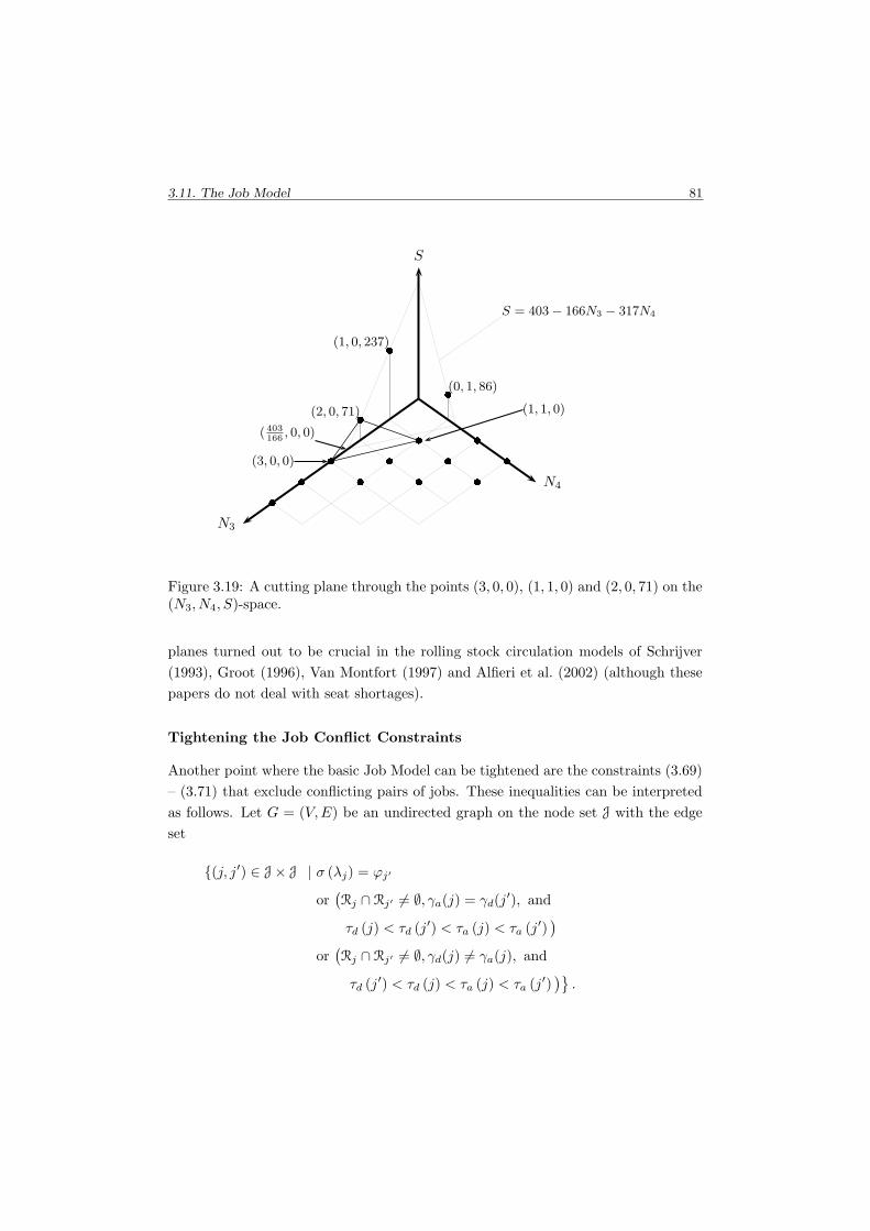
3.11. The Job Model 81
N3
N4
S
�
�
�
�
�
�
�
�
�
�
�
(2, 0, 71)
(1, 0, 237)
(0, 1, 86)
( 403166
, 0, 0)
S = 403 − 166N3 − 317N4
(3, 0, 0)
(1, 1, 0)
Figure 3.19: A cutting plane through the points (3, 0, 0), (1, 1, 0) and (2, 0, 71) on the(N3, N4, S)-space.
planes turned out to be crucial in the rolling stock circulation models of Schrijver
(1993), Groot (1996), Van Montfort (1997) and Alfieri et al. (2002) (although these
papers do not deal with seat shortages).
Tightening the Job Conflict Constraints
Another point where the basic Job Model can be tightened are the constraints (3.69)
– (3.71) that exclude conflicting pairs of jobs. These inequalities can be interpreted
as follows. Let G = (V,E) be an undirected graph on the node set J with the edge
set
{(j, j′) ∈ J × J | σ (λj) = ϕj′
or(Rj ∩ Rj′ 6= ∅, γa(j) = γd(j
′), and
τd (j) < τd (j′) < τa (j) < τa (j′))
or(Rj ∩ Rj′ 6= ∅, γd(j) 6= γa(j), and
τd (j′) < τd (j) < τa (j) < τa (j′))}
.
82 Chapter 3. Tactical Rolling Stock Circulations
Then the solutions of (3.69) – (3.71) and (3.72) are the incidence vectors of the stable
sets in G. (A stable set is a subset of nodes without any edge between them.) The
convex hull of these integer solutions is called the stable set polytope of the graph G.
When taking the linear relaxation of the model, the stable set polytope gets
relaxed to the polytope
{x ∈ [0, 1]V
∣∣ xu + xv 6 1 for each (u, v) ∈ E}
.
However, this provides a quite poor approximation of the stable set polytope, a
tighter formulation may be essential to obtain shorter solution times. Giving a tight
linear description of the stable set polytope is a topic on its own. One of the easiest
ways to sharpen the constraints is to require
∑
v∈K
xv 6 1 (3.82)
for each maximal clique in G, or at least for some of them. A maximal clique is a
containment-wise maximal subset K of nodes where each pair of members of K is
joined by an edge.
Getting Rid of Big-M Constraints
In the model (3.57) – (3.77), several units may be assigned to each job. Constraints
(3.59) are needed to set the link between the binary variables Xj and the non-
negative integer variables Nj,m. These constraints are obtained by the “big-M”
method, although the numbers µj are not that big in real-life applications: they
range from 2–5, the most frequent value is 2. We note here that in many instances
of NSR the majority of the values µj equals one; there is not much to tighten on the
constraints (3.59) then.
Constraints (3.59) concern the number of units only. An alternative way to for-
mulate the connection between variables Xj and Nj,m is to count the number of
carriages. Then constraints (3.59) are replaced by
µjXj >∑
m∈M
cmNj,m ∀j ∈ J (3.83)
where µj is an upper bound on the number of carriages that can be assigned to job
j. These are still “big-M” constraints.
The linear relaxation of “big-M” constraints is often very weak. By introducing
new decision variables as follows, constraints (3.59) or (3.83) can be eliminated. We
3.11. The Job Model 83
apply the same idea as in Section 3.8.5. For each job j, we define the set Bj ⊆ ZM+ .
Each vector b ∈ Bj represents the choice to assign bm units of type m to job j. Then
we define the binary decision variables
Yj,b ∈ {0, 1} ∀j ∈ J, b ∈ Bj
and we replace constraints (3.58) – (3.59) by the following restrictions:
Nj,m =∑
b∈Bj
bmYj,b ∀j ∈ J, m ∈ M, (3.84)
Xj =∑
b∈Bj
Yj,b ∀j ∈ J. (3.85)
Although the number of decision variables increases, the branch-and-bound process
might become faster as the linear relaxation provides better lower bounds.
3.11.5 Computational Results for the Job Model
In order to investigate the performance of the Job Model and to compare it with the
Composition Model, we consider two instances and solve them using both models
by the commercial MIP software CPLEX. The instance SPR-1 is a circulation for a
single day with 401 trips. The instance SPR-2 concerns two consecutive days with
803 trips. The timetable is based on the rolling stock type “Sprinter” of NSR. To
obtain multiple rolling stock types, we divide the available units artificially into two
types. Although the instance is not an instance of NSR, its structure is very similar
to real-life rolling stock circulation problems. The dimensions of the mixed integer
programs are given in Table 3.4 for both models and for both test instances.
Similarly to the computational test described in Section 3.10, we minimise a linear
combination of the objective criteria CKM, SKM and CCH with five different settings
(Obj1, Obj2, Obj3, Obj4, Obj5); the weight factors are given in Table 3.1.
In Section 3.11.4 we describe three ways to obtain a tighter linear relaxation of
the Job Model. The computational results below arise from an implementation where
only the tighter seat-shortage constraints are incorporated. Adding a large number
of clique inequalities of the form (3.82) did not have any effect on the solution times
and qualities. In this research we did not consider other kinds of inequalities for the
stable set polytope. Also, replacing constraints (3.59) by (3.84) – (3.84) did not have
any positive effect on the solution process.

84 Chapter 3. Tactical Rolling Stock Circulations
MIP Reduced MIP# columns # rows # columns # rows # non-zeros
CM SPR-1 36,387 16,261 33,738 15,431 167,086JM SPR-1 10,845 78,480 9,064 49,107 502,805CM SPR-2 71,202 31,406 69,546 31,292 480,773JM SPR-2 21,656 156,927 18,124 98,335 1,363,031
Table 3.4: Dimensions of the Composition Model (CM) and Job Model (JM) forinstances SPR-1 and SPR-2.
Each instance is given 1,800 seconds of CPU time. The best performance is
achieved by using for both models the CPLEX settings described in Section 3.10.1
with the exception that the linear relaxation of the Job Model is solved much faster
by the dual simplex method than by the barrier method.
We summarise the numerical computational results in Table 3.5. Each instance of
the Composition Model is solved to optimality within a couple of minutes. Observe
that the objective value of the linear relaxation hardly differs from the value of
the optimal integral solution. The optimum value of the linear relaxation of the
basic Job Model (i.e. without constraint tightening) lies 15–20% under the integer
optimum and no feasible solution is found within 1,800 seconds. Tightening the
seat-shortage constraints significantly improves the linear relaxation. Then CPLEX
is able to generate additional cuts, thereby increasing the lower bounds close to the
integer optimum: one instance has a difference of 3.11%, the lower bound in the
other instances differs from the integer optimum by less than 1.40%.
The SPR-1 instance is well-tractable by the Job Model: feasible solutions with
optimality gaps of 0–7% are found within 30 minutes. Here the optimality gap is
taken between the best integral solution and the best lower bound. The instance
SPR-2, however, turns out to be too difficult for the CPU-time limit of 30 minutes:
only one of the five objective functions admitted feasible solutions.
The Composition Model clearly outperforms the Job Model in every test instance.
Yet, it may be possible to improve the performance of the Job Model, for instance by
using a more sophisticated description of the stable set polytope. Nevertheless, we
believe that the outstanding solution times of the Composition Model are not easy
to achieve.
In addition, the Job Model strongly relies on the fact that splitting and combining
do not occur. Splitting and combining of trains makes it very difficult to describe
the jobs and to determine the conflicts between jobs. Therefore, the Job Model can
hardly be applied to instances of NSR where trains are split and combined.
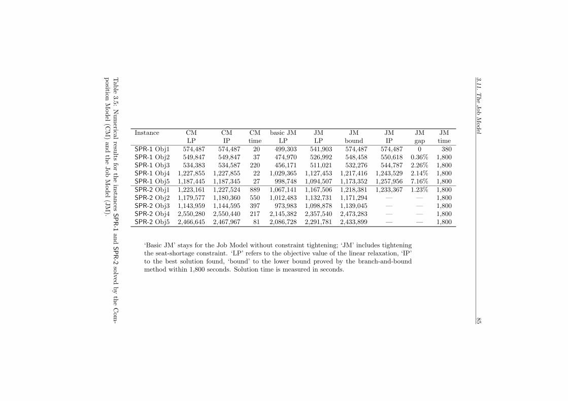
3.1
1.T
he
Job
Model
85
Instance CM CM CM basic JM JM JM JM JM JMLP IP time LP LP bound IP gap time
SPR-1 Obj1 574,487 574,487 20 499,303 541,903 574,487 574,487 0 380SPR-1 Obj2 549,847 549,847 37 474,970 526,992 548,458 550,618 0.36% 1,800SPR-1 Obj3 534,383 534,587 220 456,171 511,021 532,276 544,787 2.26% 1,800SPR-1 Obj4 1,227,855 1,227,855 22 1,029,365 1,127,453 1,217,416 1,243,529 2.14% 1,800SPR-1 Obj5 1,187,445 1,187,345 27 998,748 1,094,507 1,173,352 1,257,956 7.16% 1,800SPR-2 Obj1 1,223,161 1,227,524 889 1,067,141 1,167,506 1,218,381 1,233,367 1.23% 1,800SPR-2 Obj2 1,179,577 1,180,360 550 1,012,483 1,132,731 1,171,294 — — 1,800SPR-2 Obj3 1,143,959 1,144,595 397 973,983 1,098,878 1,139,045 — — 1,800SPR-2 Obj4 2,550,280 2,550,440 217 2,145,382 2,357,540 2,473,283 — — 1,800SPR-2 Obj5 2,466,645 2,467,967 81 2,086,728 2,291,781 2,433,899 — — 1,800
‘Basic JM’ stays for the Job Model without constraint tightening; ‘JM’ includes tighteningthe seat-shortage constraint. ‘LP’ refers to the objective value of the linear relaxation, ‘IP’to the best solution found, ‘bound’ to the lower bound proved by the branch-and-boundmethod within 1,800 seconds. Solution time is measured in seconds.
Tab
le3.5:
Num
ericalresu
ltsfor
the
instan
cesSPR-1
and
SPR-2
solvedby
the
Com
-position
Model
(CM
)an
dth
eJob
Model
(JM
).

86 Chapter 3. Tactical Rolling Stock Circulations
3.12 Conclusions
In this chapter, we considered the tactical rolling stock circulation problem of NSR
and we described two ways of modelling it. The models can express various technical
and market requirements. In computational experiments, the Composition Model
provided good solutions with reasonable running times, the Job Model performed
much worse.
We tested the Composition Model on fairly large instances of NSR. The model
turned out to be robust enough to cope with very different weights on the objective
criteria. When solved by a commercial MIP solver, it provided rolling stock circula-
tions with different objective characteristics in a couple of hours of computation time.
The decision makers can choose a solution that matches the practical requirements
best. Planners at NSR agreed that the solutions of the Composition Model are in
any respect better than the manually created plans.
The computer-generated rolling stock circulations must still be checked and some-
times adjusted by human planners. Nevertheless, the implemented model turned out
to be a very useful planning tool at the Logistics Department of NSR. From 2004 on,
the basic shape of the tactical rolling stock circulations at NSR are partly computed
by solving this model. These computer-generated circulations have a significantly
lower number of carriage-kilometres than the plan of the previous years while pro-
viding the same service quality. This allowed NSR to reduce its annual operational
costs by a couple of millions of euros.

Chapter 4
Maintenance Routing
Short-term planning at NSR includes a number of planning steps that are currently
carried out without computer-aided planning tools. Of these problems of railway
practise, we only study the maintenance routing problem of NSR in this thesis. Main-
tenance routing makes sure that rolling stock units that need a regular preventive
maintenance check visit the maintenance facility in time.
We present two integer programming models for maintenance routing. The ‘Inter-
change Model’ is designed to take as many details of reality into account as possible.
However, the large amount of input data needed for the Interchange Model is difficult
to obtain. This motivates the ‘Transition Model’ which is a much simpler formulation
of the problem. Implementations of real-life test data give promising results for both
models: we find good solutions in an acceptable amount of time.
This chapter is structured as follows. First we describe the maintenance routing
process of NSR in detail and formulate the maintenance routing problem. Thereafter
we give a brief literature overview. Subsequently we describe the Interchange Model
and the Transition Model. For both models, we discuss theoretical complexity issues
and computational results on test instances of NSR. At the end of the chapter, we
draw some conclusions.
4.1 Maintenance Routing in Practise
The operational rolling stock plan only concerns duties for anonymous units. In short-
term planning in practise, at most 3 days before executing the operational plan the
physical units are assigned to the duties. This gives the regular plan which describes
87

88 Chapter 4. Maintenance Routing
what the individual units have to do during the forthcoming couple of days. The
regular plan is composed of a rolling stock circulation and a corresponding shunting
plan. Details of the shunting plans are only known to local planners. From the
central planners’ point of view, the regular plan is a rolling stock circulation that
admits a shunting plan.
A task is a smallest indivisible train movement in the regular plan to be carried
out by a single unit. So, if a trip is assigned a composition with more than one unit,
it corresponds to several tasks. A pair (t, t′) of tasks is a regular transition if t′ is
the successor of task t. That is, t and t′ are carried out consecutively by the same
unit in the regular plan. A regular duty is the sequence of all tasks of a single unit
during the forthcoming days.
Units require a preventive maintenance check after a certain number of kilometres.
This limit depends on the rolling stock type; if a unit travelled that distance since its
last maintenance check, then it may not carry passengers any more before undergoing
a maintenance check. Units visit the maintenance facility roughly once a month. Note
that units must also undergo smaller safety inspections once every two days. These
can take place at many stations and are handled on an ad hoc basis by local planners.
These small safety inspections are not considered in this chapter at all.
Maintenance of rolling stock is carried out by NedTrain while NSR is responsible
for sending units to the maintenance facilities in time. The checks take about a
day and can only take place at specialised stations. In tactical and operational
planning, maintenance is taken into account in a limited way. The timetable contains
maintenance tasks; if a unit is assigned to such a task, it undergoes a maintenance
check. However, this assignment is done provisionally, without caring about which
unit will be urgent and when. The actual maintenance routing is handled in the short-
term phase by central planners at the Materieelregelcentrum (MRC). Maintenance
routing is carried out every day with a rolling planning horizon, always considering
the forthcoming 1–3 days.
Every day, maintenance routing planners receive the list of the urgent units: those
units that need a maintenance check within the planning horizon. Usually, these are
the units that made the highest number of kilometres since their last maintenance
check. These units may have different urgencies, expressed by a deadline (for instance,
saying that the maintenance check should take place within 2 days). Maintenance
routing has to make sure that the urgent units carry out a maintenance task within
the planning horizon. To that end, the part of the regular plan that lies within the
planning horizon must be adjusted.
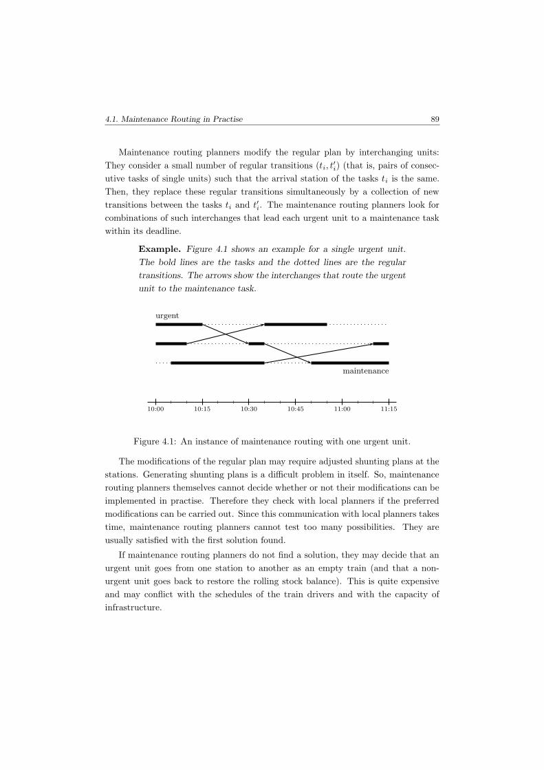
4.1. Maintenance Routing in Practise 89
Maintenance routing planners modify the regular plan by interchanging units:
They consider a small number of regular transitions (ti, t′i) (that is, pairs of consec-
utive tasks of single units) such that the arrival station of the tasks ti is the same.
Then, they replace these regular transitions simultaneously by a collection of new
transitions between the tasks ti and t′i. The maintenance routing planners look for
combinations of such interchanges that lead each urgent unit to a maintenance task
within its deadline.
Example. Figure 4.1 shows an example for a single urgent unit.
The bold lines are the tasks and the dotted lines are the regular
transitions. The arrows show the interchanges that route the urgent
unit to the maintenance task.
10:00 10:15 10:30 10:45 11:00 11:15
urgent
maintenance
Figure 4.1: An instance of maintenance routing with one urgent unit.
The modifications of the regular plan may require adjusted shunting plans at the
stations. Generating shunting plans is a difficult problem in itself. So, maintenance
routing planners themselves cannot decide whether or not their modifications can be
implemented in practise. Therefore they check with local planners if the preferred
modifications can be carried out. Since this communication with local planners takes
time, maintenance routing planners cannot test too many possibilities. They are
usually satisfied with the first solution found.
If maintenance routing planners do not find a solution, they may decide that an
urgent unit goes from one station to another as an empty train (and that a non-
urgent unit goes back to restore the rolling stock balance). This is quite expensive
and may conflict with the schedules of the train drivers and with the capacity of
infrastructure.
90 Chapter 4. Maintenance Routing
4.2 Maintenance Strategy
We described above the maintenance routing process at NSR; our research addresses
this problem. However, other maintenance strategies are also possible and they would
lead to routing problems of other type.
One might wonder whether the entire maintenance routing process could be elimi-
nated at all by taking maintenance considerations in earlier phases of the rolling stock
planning into account. That is, whether it would make sense to create a rolling stock
circulation for a month such that each unit visits the maintenance facility exactly
once. This is the usual approach in the airline industry.
The answer is that it would not work at NSR. First, it would mean that one has to
consider individual units in tactical and operational circulations. Due to the size and
complexity of the problem, the computation times at these planning phases would
probably become huge. Second, even if we had time for all these long computations,
disruptions and delays in the operations would make it unlikely that the rolling stock
schedule can be carried out exactly as planned in a period longer than a couple of
days. So, we need short planning horizons in maintenance routing.
Fortunately, the Dutch railway network contains a large number of frequently
operated and relatively short train lines. This provides many interchange possibilities
for the units. Therefore, as experience shows, a couple of days is usually enough to
route an urgent unit to a maintenance facility. This explains why the maintenance
routing planners consider a planning horizon of 1 to 3 days and only a small number
of urgent units to be routed.
In the current maintenance practise, NSR and NedTrain agree on the number of
maintenance tasks in an early phase of the planning process. In short-term planning,
all these maintenance tasks must be filled with a unit even if no unit is close to
the kilometre-limit. Studies at NSR showed that more maintenance is carried out
currently than strictly necessary.
Alternative maintenance strategies may help to reduce maintenance costs. A
natural idea is to send a unit to a maintenance task only if it really has reached the
kilometre-limit (or if it is broken). Central coordination is still needed for the case
when too many units would require a maintenance check on the same day. A key
element is to make routing decisions as late as possible. To that end, one might even
accept a higher number of empty trains. The long-time benefit of such an alternative
maintenance strategy is currently being investigated at NSR and NedTrain. Changing
the maintenance strategy requires significant adjustments in tactical, operational

4.3. Problem Formulation 91
and short-term rolling stock planning. Nonetheless, we believe that the modelling
approaches of this chapter can be carried over for altered problem specifications.
4.3 Problem Formulation
In this section, we give a (slightly vague) formulation of the maintenance routing
problem. It is rather a list of wishes that must be taken into account in models for
the problem.
The maintenance routing problem amounts to modifying the regular rolling stock
duties such that the following requirements are satisfied.
1. The new duty of each urgent unit contains a maintenance task within the
deadline.
2. Empty trains are to be avoided as much as possible.
3. Passenger traffic may not suffer from maintenance routing. In particular, each
task in the timetable must be covered by a unit.
4. The rolling stock circulations should not be affected too much. To ensure that,
maintenance routing planners only interchange units of the same type. In other
words, maintenance routing handles the different rolling stock types separately.
5. In order to agree quickly with local planners on the modified shunting plans,
maintenance routing should not require too many changes in the shunting plans.
We emphasise again that maintenance routing planners do not have direct
information about the shunting process. Based on their experience, however,
they can mostly guess quite well whether or not interchanging a couple of units
at a given station is likely to be approved by local planners.
The fifth requirement above is not well-defined yet. It is not clear at all how one
should measure the deviation from the regular shunting plan without even knowing
it in detail. The models we are going to describe in this chapter show two radically
different ways to do it.
The requirements become less and less binding as time approaches the point
when the trains have to run. In real-life maintenance routing at NSR, the third and
fourth requirements may actually be violated if no other solution is found. Timetable
services may be operated with a smaller number of units than planned, trains may
even be cancelled. Also, units of different types are interchanged. Both kinds of
violations are strongly undesirable and used only as a last option.

92 Chapter 4. Maintenance Routing
The objective criteria of tactical planning (see Section 3.6) are not really im-
portant any more. Instead, the main goal is to find quickly a solution that can be
smoothly implemented in practise. There is no natural quantity to measure how good
a solution is. Different maintenance planners may judge the same solution differently.
Therefore, there is quite a choice for an objective function in mathematical models.
Important is that the objective function implements the main goals listed above and
that most maintenance planners find the solutions reasonably good.
Using any method in short-term planning, there is not enough time to plan the
rolling stock from scratch mainly because the modified shunting plans cannot be
checked easily. But we may use the fact that we have the regular plan for which
feasible shunting plans exists. Applying a small number of modifications, one may
hope that the shunting plans can in fact be adjusted.
Each solution of maintenance routing needs approval of the local planners. There-
fore, the final goal of this research is to develop an interactive decision support system
that proposes candidate solutions to maintenance routing planners: they can accept
the proposal or run the system again with modified specifications. Results on single
instances can also be used to refine the models. In real-life maintenance planning,
local planners must be contacted several times until a solution is approved. So, it is
essential to produce candidate solutions quickly. Waiting 15 minutes or more would
slow down the planning process. Moreover, methods that provide reasonably good
solutions quickly are much more likely to be accepted both by decision makers and
by maintenance routing planners themselves.
Finally, reality is always much more complex than what mathematical models can
describe effectively. In case of emergency, almost every rule may be violated. Having
this in mind, we focused in our models and test implementations on the rules rather
than on the exceptions. Then the models may become slightly rigid. Nonetheless,
if computer models can help in solving the easy but time-consuming maintenance
routing instances, then the planners have more time to deal with instances that
really require creativity and ad hoc ideas.
The input for the maintenance routing problem contains the set of tasks. A task t
is characterised by the departure station sd (t), arrival station sa (t), departure time
τd (t) and arrival time τa (t) (so τd (t) 6 τa (t)). The successor task of task t is σ (t).
The pair (t, σ (t)) is a regular transition; regular transitions satisfy sa (t) = sd (σ (t))
and τa (t) < τd (σ (t)). We assume that each task lies entirely within the planning
horizon. If a task in a railway application departs earlier than the beginning of the
planning horizon, we set its departure time to the beginning of the planning period.
Similarly, we cut off the parts of tasks after the end of the planning horizon.

4.4. Literature Overview 93
The input also specifies the set of urgent units and the set of maintenance tasks.
For each urgent unit u, the set of those maintenance tasks is given that can be
assigned to u; these sets may express different urgencies. Finally, we assume that the
number of urgent units equals the number of maintenance tasks.
4.4 Literature Overview
Ziarati et al. (1997) set up a large-scale integer programming model for locomotive
assignment where maintenance routing plays an important role. Lingaya et al. (2002)
describe a model for supporting the operational management of locomotive-hauled
railway cars. They seek for a maximum expected profit schedule that satisfies various
constraints, among them also maintenance requirements.
Other papers focus on aircraft maintenance routing. For example, Barnhart et al.
(1998a), Clarke et al. (1997), Feo and Bard (1989), Gopalan and Talluri (1998) and
Talluri (1998) deal with this problem. Anderegg et al. (2003) describe models for
railway applications that are similar to the aircraft routing models.
These models consider maintenance routing as a part of the medium- and long-
term vehicle scheduling problem. Small safety inspections (that are arranged at NSR
by the local planners on an ad hoc basis) form an important part of the problem
specification and also the larger-scale maintenance checks are taken into account.
These models compute the vehicle circulation for the forthcoming month such that
each vehicle is scheduled for maintenance exactly once. Also, the vehicle schedules are
created from scratch, without taking shunting into account. Therefore, in a railway
application there is just a small probability that the output of the models in the
literature can be carried out in practise.
4.5 The Interchange Model
The basic decision of maintenance routing planners is to consider a number of tasks
and to re-arrange the successors of these tasks. The set of all such simultaneous
interchanges can be very large. In fact, each modified plan can be interpreted as a
large simultaneous interchange. In order to keep the size of the model tractable, we
consider only a relatively small set of elementary modifications called ‘interchanges’.
An essential part of the model in this section is that interchanges can be combined,
that is, interchanges can be carried out after each other. Then solutions with complex
patterns can be obtained by using the interchanges as building blocks.

94 Chapter 4. Maintenance Routing
4.5.1 Input and the Output of the Interchange Model
The input of the model contains the list of allowed modifications of the regular
plan. We assume that these allowed modifications have a special form, we call them
‘interchanges’. An interchange describes which unit should take over the role of
which other unit and it specifies exactly when this must take place. We make several
assumptions about interchanges.
An interchange is specified by two time moments m1 < m2 in the planning
period, by k > 2 regular transitions (ti, σ (ti)) and by a permutation I : {1, . . . , k} →
{1, . . . , k}. For each i = 1, . . . , k, we require
τa (ti) 6 m1,
m2 6 τd (σ (ti)) .
In other words, for each i = 1, . . . , k, the time interval [m1,m2] is contained in the
time interval between the tasks ti and σ (ti).
A single rule i → I(i) of an interchange is interpreted as follows. The unit
that arrived as task ti keeps its planned position on the shunting yard till moment
m1. Then it is repositioned to the place where another unit is stored according
to the shunting plan: this other unit was planned to carry out task σ(tI(i)
). The
repositioning is ready at the moment m2: from that moment on, the original shunting
plan is executed again. When all rules of an interchange are applied, each task is
covered by a unit.
The time difference m2 −m1 must be enough to carry out the necessary shunting
operations, so it may not be shorter than a certain buffer time %. Assuming that
% minutes are enough for the extra shunting, we only allow interchanges where the
difference m2 − m1 equals %. Based on discussion with planners, we set % to 10
minutes.
We also assume that for each single interchange, the shunting plans can in fact
be modified so that the interchange is carried out. That is, that the individual inter-
changes are approved by local planners or at least by maintenance routing planners.
However, we do not know which combinations of interchanges can be carried out
together.

4.5. The Interchange Model 95
Example. Figure 4.2 indicates three units that arrive according to
the regular plan at a station and depart from there later. In this
example the buffer time equals to 10 minutes. The interchange is
described by the given tasks and by
m1 = 10:00, m2 = 10:10,
1 → I(1) = 2, 2 → I(2) = 3 and 3 → I(3) = 1.(4.1)
As one can see in Figure 4.2, the same interchange structure between
the same three units may also take place 10 minutes later. In the
input, it is represented by another interchange with m1 = 10:10,
m2 = 10:20 and with the same interchange rules as in (4.1).
t1
t2
t3
σ (t1)
σ (t2)
σ (t3)
9:30 10:00 10:30 11:00
Figure 4.2: An example of an interchange.
This is a basic notion of interchanges. In our implementations, we used a slightly
extended version of interchanges that is described in Section 4.5.4. Here we restricted
ourselves to this basic notion for the sake of a simpler, more intuitive notation.
Applying one interchange only provides very limited possibilities. So, we wish to
combine interchanges in order to model shunting in a more flexible way.
Definition 4.1. Two interchanges given by (t1, . . . , tk, I,m1,m2) and (t′1, . . . , t′k′ ,
I ′, m′1, m′
2) are independent if the sets of tasks {t1, . . . , tk} and {t′1, . . . , t′k′} are
disjoint or if the time intervals [m1;m2] and [m′1;m
′2] are disjoint.
In this model of the shunting process, only pair-wise independent interchanges
can be combined. This can be motivated as follows. From the maintenance routing
planners’ perspective, it is difficult to check whether several interchanges together
can be implemented in practise. By using independent interchanges, we localise their
effects on the regular plan, making it more likely that the entire new plan can be
carried out. It is possible that a combination of certain non-independent interchanges
96 Chapter 4. Maintenance Routing
can still be carried out, it may even decrease the number of shunting movements.
As the information about local shunting possibilities is limited, we do not allow such
non-independent interchanges to stay on the safe side.
It is interesting to compare this shunting model to that in Section 3.3 (also used
in Chapter 5). In tactical (and also operational planning), the order of the units
on the shunting yards is not considered at all. In contrary, we assume that every
composition change is possible. In short-term planning, however, we keep track of
the position of every individual unit.
The input of the Interchange Model contains a penalty value for each interchange,
expressing how much additional shunting effort it causes. These penalties also re-
flect the likelihood that the interchange can be carried out successfully: more risky
interchanges get higher penalties. In Section 4.5.5 we will discuss how we can obtain
a list of interchanges and penalty values.
The output of the model is a collection of independent interchanges such that
applying them, the urgent units reach an appropriate maintenance task. We can
interpret this output as a collection of new duties (i.e. chains of tasks) for the units
plus suggestions to local planners how the new rolling stock plan can be implemented
in practise.
4.5.2 Graph Representation
We give a flow-type model for the maintenance routing problem, thus we first need
a graph G = (V,A). The units are labelled by d = 1, . . . , D. Index the integer
minutes in the planning period by 0, . . . , H. Create a node for every pair (d,m) with
d ∈ {1, . . . , D} and m ∈ {0, . . . , H} such that m does not lie strictly between the
departure time and the arrival time of any task which is carried out by unit d. For a
node v = (d,m), let time(v) := m. First nodes are the nodes with time(v) = 0, last
nodes are those with time(v) = H. Let V0 denote the set of first nodes and V∞ the
set of last nodes.
For any task t which is carried out by unit d, insert a task arc from (d, τd (t))
to (d, τa (t)). Moreover, for each d ∈ {1, . . . , D} and for each m ∈ {0, . . . , H}, join
node (d,m) to (d,m + 1) if these nodes exist and if they are not yet joined by a task
arc. The arcs defined so far are called regular arcs. They form a collection of disjoint
directed paths, each path representing the regular duty of one unit.
Each node (d,m) of the graph refers to a station as follows. Unit d has a latest
arrival event as task t before m or it has an earliest departure event as task t′ after

4.5. The Interchange Model 97
m. Then node v = (d,m) refers to sa (t) or sd (t′), whichever of them exists; this
station is denoted by stat(v). Note that if both t and t′ exist, then sa (t) = sd (t′).
Let I denote the set of interchanges. Consider an interchange C = (t1, . . . , tk, I,
m1,m2) ∈ I. For each i = 1, . . . , k, let vi = (di,m1) and wi = (di,m2) where
di is the unit that carries out tasks ti and σ (ti) in the regular plan. Create for
each i = 1, . . . , k an interchange arc (vi, wI(i)) and identify C with the set of arcs
{(vi, wI(i)) | i = 1, . . . , k}. If a particular pair (v, w) is an interchange arc in several
interchanges, we have parallel arcs from v to w.
Independence of interchanges is defined in Definition 4.1. In this graph represen-
tation of the problem, the definition can be stated as follows.
Definition 4.2. Let C = {(vi, wI(i)) | i = 1, . . . , k} and C ′ = {(v′i, w
′I′(i)) | i =
1, . . . , k′} be interchanges. Let P be the union of the arc sets of those regular arc
paths that connect the nodes vi to the nodes wi. Let P ′ be defined similarly for the
interchange C ′. Then C and C ′ are said to be independent if the arc sets P and P ′
are disjoint.
The arcs of the graph have weights to estimate the shunting effort of the inter-
changes. For each interchange arc a, set weight(a) to the penalty of the complete
interchange containing arc a. The weight of the regular arcs is zero.
Example. Figure 4.3 shows the graph for the six tasks in Fig-
ure 4.2 and the interchange in (4.1). Horizontal arcs are regular,
the six task arcs are denoted by t1, t2, t3 and σ (t1) , σ (t2) , σ (t3).
The interchange is represented in the graph by the arcs e, f, g.
t1
t2
t3
σ (t1)
σ (t2)
σ (t3)
9:30 10:00 10:30 11:00
g f
e
Figure 4.3: The graph representation of the interchange in Figure 4.2.
Let U be the set of nodes (u, 0) where u ∈ {1, . . . , D} is the index of an urgent
unit. We identify the urgent units with the nodes in U . For each maintenance task
that is carried out in the regular plan by unit d and that starts at time moment
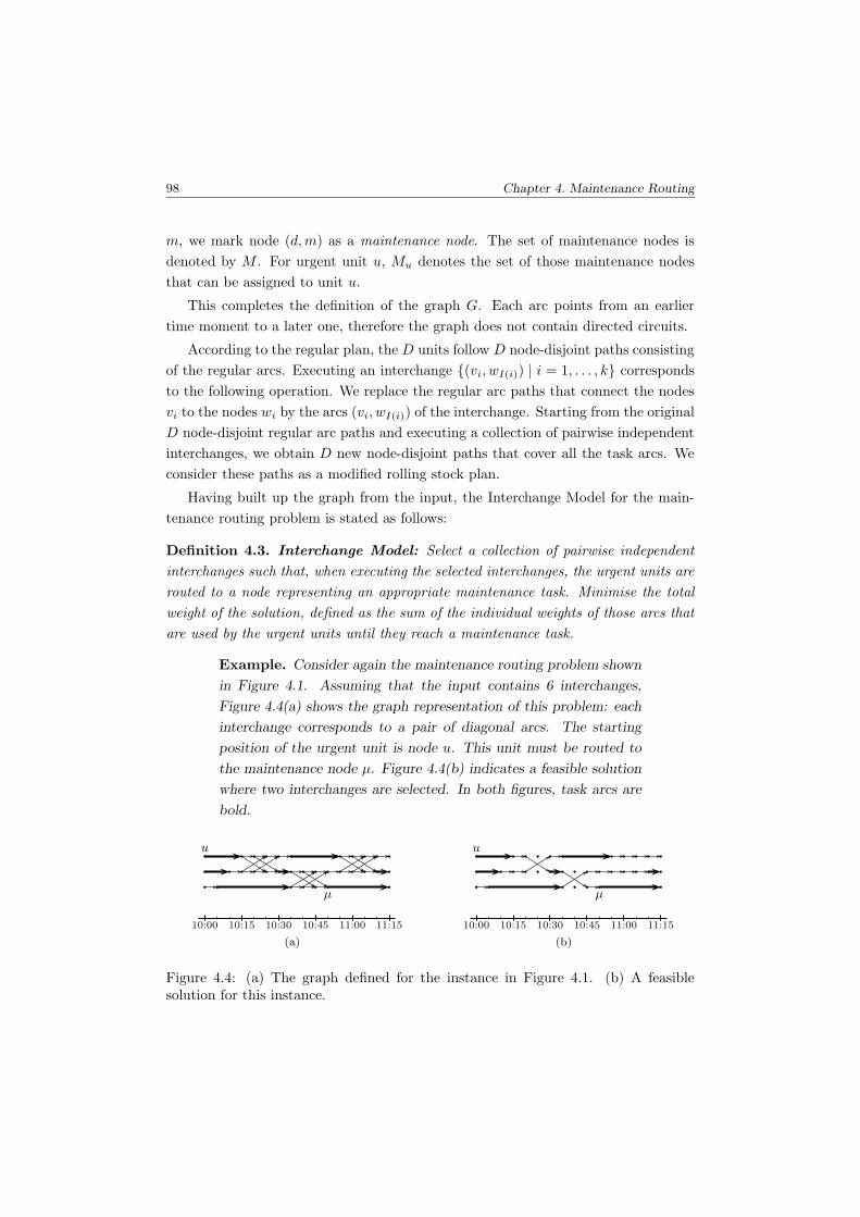
98 Chapter 4. Maintenance Routing
m, we mark node (d,m) as a maintenance node. The set of maintenance nodes is
denoted by M . For urgent unit u, Mu denotes the set of those maintenance nodes
that can be assigned to unit u.
This completes the definition of the graph G. Each arc points from an earlier
time moment to a later one, therefore the graph does not contain directed circuits.
According to the regular plan, the D units follow D node-disjoint paths consisting
of the regular arcs. Executing an interchange {(vi, wI(i)) | i = 1, . . . , k} corresponds
to the following operation. We replace the regular arc paths that connect the nodes
vi to the nodes wi by the arcs (vi, wI(i)) of the interchange. Starting from the original
D node-disjoint regular arc paths and executing a collection of pairwise independent
interchanges, we obtain D new node-disjoint paths that cover all the task arcs. We
consider these paths as a modified rolling stock plan.
Having built up the graph from the input, the Interchange Model for the main-
tenance routing problem is stated as follows:
Definition 4.3. Interchange Model: Select a collection of pairwise independent
interchanges such that, when executing the selected interchanges, the urgent units are
routed to a node representing an appropriate maintenance task. Minimise the total
weight of the solution, defined as the sum of the individual weights of those arcs that
are used by the urgent units until they reach a maintenance task.
Example. Consider again the maintenance routing problem shown
in Figure 4.1. Assuming that the input contains 6 interchanges,
Figure 4.4(a) shows the graph representation of this problem: each
interchange corresponds to a pair of diagonal arcs. The starting
position of the urgent unit is node u. This unit must be routed to
the maintenance node µ. Figure 4.4(b) indicates a feasible solution
where two interchanges are selected. In both figures, task arcs are
bold.
u
µ
10:00 10:15 10:30 10:45 11:00 11:15
(a)
u
µ
10:00 10:15 10:30 10:45 11:00 11:15
(b)
Figure 4.4: (a) The graph defined for the instance in Figure 4.1. (b) A feasiblesolution for this instance.
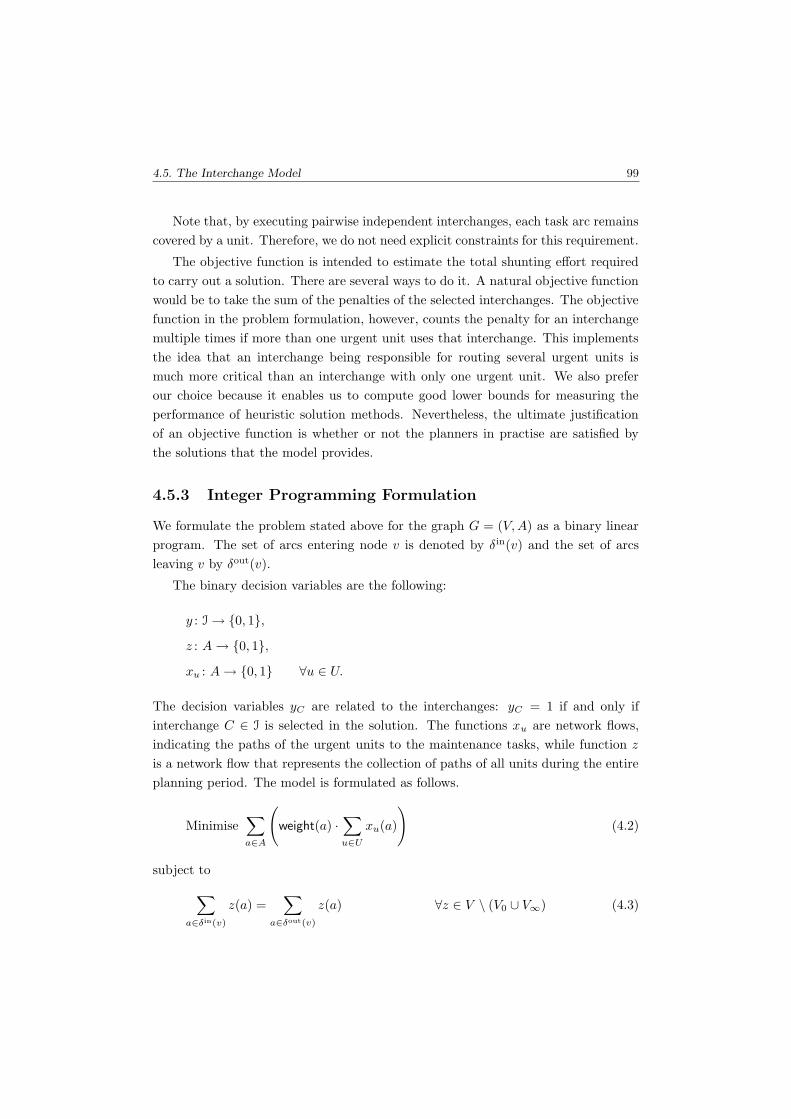
4.5. The Interchange Model 99
Note that, by executing pairwise independent interchanges, each task arc remains
covered by a unit. Therefore, we do not need explicit constraints for this requirement.
The objective function is intended to estimate the total shunting effort required
to carry out a solution. There are several ways to do it. A natural objective function
would be to take the sum of the penalties of the selected interchanges. The objective
function in the problem formulation, however, counts the penalty for an interchange
multiple times if more than one urgent unit uses that interchange. This implements
the idea that an interchange being responsible for routing several urgent units is
much more critical than an interchange with only one urgent unit. We also prefer
our choice because it enables us to compute good lower bounds for measuring the
performance of heuristic solution methods. Nevertheless, the ultimate justification
of an objective function is whether or not the planners in practise are satisfied by
the solutions that the model provides.
4.5.3 Integer Programming Formulation
We formulate the problem stated above for the graph G = (V,A) as a binary linear
program. The set of arcs entering node v is denoted by δin(v) and the set of arcs
leaving v by δout(v).
The binary decision variables are the following:
y : I → {0, 1},
z : A → {0, 1},
xu : A → {0, 1} ∀u ∈ U.
The decision variables yC are related to the interchanges: yC = 1 if and only if
interchange C ∈ I is selected in the solution. The functions xu are network flows,
indicating the paths of the urgent units to the maintenance tasks, while function z
is a network flow that represents the collection of paths of all units during the entire
planning period. The model is formulated as follows.
Minimise∑
a∈A
(weight(a) ·
∑
u∈U
xu(a)
)(4.2)
subject to
∑
a∈δin(v)
z(a) =∑
a∈δout(v)
z(a) ∀z ∈ V \ (V0 ∪ V∞) (4.3)

100 Chapter 4. Maintenance Routing
∑
a∈δout(v)
z(a) = 1 ∀v ∈ V0 (4.4)
∑
a∈δin(v)
z(a) 6 1 ∀z ∈ V (4.5)
∑
a∈δout(v)
z(a) 6 1 ∀z ∈ V (4.6)
∑
a∈δin(v)
xu(a) =∑
a∈δout(v)
xu(a) ∀u ∈ U, v ∈ V \ ({u} ∪ Mu) (4.7)
∑
a∈δout(v)
xu(a) = 1 ∀u ∈ U (4.8)
∑
u∈U
∑
a∈δout(v)
xu(a) = 0 ∀v ∈ M (4.9)
∑
u∈U :v/∈Mu
∑
a∈δin(v)
xu(a) = 0 ∀v ∈ M (4.10)
∑
u∈U
xu(a) 6 z(a) ∀a ∈ A (4.11)
z(a) = yC ∀C ∈ I, a ∈ C (4.12)
z(a) ∈ {0, 1} ∀a ∈ A (4.13)
xu(a) ∈ {0, 1} ∀u ∈ U, a ∈ A (4.14)
yC ∈ {0, 1} ∀C ∈ I (4.15)
Constraints (4.3) and (4.4) state that the function z is a network flow where the
first nodes are sources of value 1 and where the last nodes are the sinks. Constraint
(4.5) and (4.6) make sure that every node has a throughput of at most 1 in this flow.
Then the arcs with z(a) = 1 form a system of node-disjoint paths, connecting the
first nodes to the last nodes.
Similarly, constraints (4.7) and (4.8) express that the functions xu are network
flows such that u is the only source node and that the nodes in Mu are the sinks.
Constraints (4.9) make sure that no flow leaves the maintenance nodes in any of the
network flows xu. Moreover, (4.10) states that a maintenance node v may have in-
coming flow only in a flow xu if v is an allowed maintenance node for urgent unit u.
According to constraints (4.11), the paths indicated by the flows xu form a subsystem
of the path system indicated by the network flow z. Constraints (4.12) express that
either all arcs of an interchange are selected for the network flow z or none of them.
Finally, constraints (4.13) – (4.15) set the domains of the variables.

4.5. The Interchange Model 101
The binary integer program does not have any explicit constraints saying that
the selected interchanges should be independent. The following lemma states that
such constraints are not necessary.
Lemma 4.4. Consider any feasible solution of the model (4.2) – (4.15). Then for
any interchange C = {(vi, wI(i)) | i = 1, . . . , k} with yC = 1 and for i = 1, . . . , k, the
regular arc path between nodes vi and wi does not contain a node v /∈ {vi, wi} such
that v is traversed by the flow z.
Proof. Suppose there exists an interchange C with yC = 1 and a node v = (d,m) lying
between nodes vi and wi that is traversed by z (see Figure 4.5). Choose such a pair
(C, v) so that m is as small as possible. Then the nodes strictly between vi and v have
no throughput in z. Let e be the arc entering node v with z(e) = 1. This arc e cannot
be a regular arc, so e ∈ C ′ for some interchange C ′ = {(v′j , w
′I′(j)) | j = 1, . . . , k′}.
This interchange C ′ must contain an arc f with z(f) = 1 that leaves a node (d,m′)
with m′ < m. The tail of arc f is traversed by z, therefore time(tail(f)) 6 time(vi).
(Here, tail(f) denotes the tail of arc f .) Moreover, vi 6= tail(f), since otherwise node
vi would have an outflow in z larger than 1. Thus we have time(tail(f)) < time(vi).
Then interchange C ′ has yC′ = 1, node vi is traversed by z and lies between v′j
and w′j for an index j that satisfies v = w′
j . This contradicts the choice of interchange
C and node v. �
v′
j
v = w′
j
vi vi
C′3 f
C′3 e
Figure 4.5: Illustration for the proof of Lemma 4.4. Bold arcs have z-value 1.
Lemma 4.4 immediately implies
Corollary 4.5. Let (x, y, z) be a feasible solution of the binary integer program (4.2)
– (4.15) and suppose that yC1= yC2
= 1 for interchanges C1, C2 ∈ I. Then C1 and
C2 are independent.
Thus, in every feasible solution of the binary linear program, the set of arcs with
z(a) = 1 arises from the regular transitions by executing the interchanges with yC = 1
and these interchanges are pairwise independent. Therefore, every feasible solution
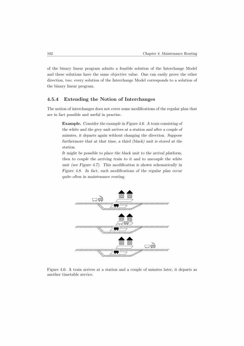
102 Chapter 4. Maintenance Routing
of the binary linear program admits a feasible solution of the Interchange Model
and these solutions have the same objective value. One can easily prove the other
direction, too: every solution of the Interchange Model corresponds to a solution of
the binary linear program.
4.5.4 Extending the Notion of Interchanges
The notion of interchanges does not cover some modifications of the regular plan that
are in fact possible and useful in practise.
Example. Consider the example in Figure 4.6. A train consisting of
the white and the grey unit arrives at a station and after a couple of
minutes, it departs again without changing the direction. Suppose
furthermore that at that time, a third (black) unit is stored at the
station.
It might be possible to place the black unit to the arrival platform,
then to couple the arriving train to it and to uncouple the white
unit (see Figure 4.7). This modification is shown schematically in
Figure 4.8. In fact, such modifications of the regular plan occur
quite often in maintenance routing.
Figure 4.6: A train arrives at a station and a couple of minutes later, it departs asanother timetable service.
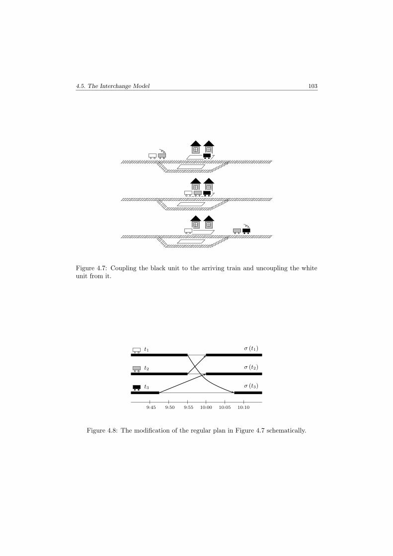
4.5. The Interchange Model 103
Figure 4.7: Coupling the black unit to the arriving train and uncoupling the whiteunit from it.
9:45 9:50 9:55 10:00 10:05 10:10
σ (t1)
σ (t2)
σ (t3)
t1
t2
t3
Figure 4.8: The modification of the regular plan in Figure 4.7 schematically.

104 Chapter 4. Maintenance Routing
The modification in the example above does not comply with the definition of
interchanges if the time difference between the arrival and departure is less than the
buffer time %. This motivates to extend the notion of interchanges.
For tasks t1, . . . tk, let
α := max{τa (t1) : i = 1, . . . , k},
β := min{τd (σ (t1)) : i = 1, . . . , k}.
So far, we allowed interchanges (t1, . . . , tk, I,m1,m2) with m2 = m1 +% if β−α > %.
We now introduce interchanges for the case α < β < α + %. That is, the time
intervals [τa (ti) ; τd (σ (ti))] intersect but the intersection is shorter than % minutes.
We require for an extended interchange between tasks ti and σ (ti) for i = 1 . . . , k
the following:
τa (ti) = α or τa (ti) 6 β − % ∀i = 1, . . . , k,
τd (σ (ti)) = β or τd (σ (ti)) > α + % ∀i = 1, . . . , k.
That is, the arrival time of a task is either exactly the latest arrival time or it is
smaller than the earliest departure time minus the buffer time. A similar restriction
is stated for the departure times. The interchanges defined in Section 4.5.1 satisfy
this definition. Note that although not part of the definition, non-basic interchanges
are only intended to model the case where all tasks with arrival time α belong the
one trip, and also all tasks with departure time β belong the one trip. Such a case is
shown in Figures 4.7 and 4.8.
Just like in Section 4.5.1, the substantial content of an extended interchange is
described by the permutation I : {1, . . . , k} → {1, . . . , k} which indicates how the
modified plan matches tasks t1, . . . , tk to the tasks σ (t1) , . . . , σ (tk).
Extended interchanges can easily be added to the graph defined in Section 4.5.2.
Suppose that tasks t1, . . . , tk form an extended interchange with α > β − % (i.e.
they cannot form a basic interchange) and suppose that for each i = 1, . . . , k, task
ti is carried out by unit di in the regular plan. Then we represent the extended
interchange with the following set of arcs:
from node (di,max{α;β − %}) to node(dI(i),min{β;α + %}
).
Again, we identify the extended interchange with this set of arcs in the graph. The
graph representation of the extended interchange considered above is given in Fig-
ure 4.9.

4.5. The Interchange Model 105
9:45 9:50 9:55 10:00 10:05 10:10
σ (t1)
σ (t2)
σ (t3)
t1
t2
t3
Figure 4.9: The modification of the regular plan indicated in Figure 4.7 is representedin the graph.
Using extended interchanges, the formulation of the Interchange Model and the
binary linear program (4.2) – (4.15) remain unchanged; independence of interchanges
is defined by Definition 4.2. Then each claim about the binary program, in particular
Corollary 4.5, can be proved without any change.
We emphasise two important properties of extended interchanges in the graph
representation of the problem.
1. For an extended interchange {(vi, wI(i)) | i = 1, . . . , k}, the time intervals
[time(vi); time(wi)] intersect.
2. If an extended interchange contains two arcs a1 and a2 such that the tail of
a1 refers to an earlier time moment than the tail of a2 does (formally: if
time(tail(a1)) < time(tail(a2))) then the tail of a2 is the head of a task arc.
Similarly, if time(head(a1)) < time(head(a2)) then the head of a1 is the tail
node of a task arc.
4.5.5 Obtaining the Input Data
The Interchange Model requires a large amount of information about the shunting
process. Collecting all these details is not easy. Another problem is to define appro-
priate numerical penalty values: Different local planners may judge the difficulty of
certain interchanges quite differently.
For our test implementation, we create the interchanges ourselves using the ex-
tended notion of interchanges. First we specify the buffer time. As mentioned,
discussions with the planners lead to a value of 10 minutes. Then we look for pairs
106 Chapter 4. Maintenance Routing
of tasks t1 and t2 with
sa (t1) = sa (t2) ,
τa (t1) 6 τd (σ (t2)) − %,
τa (t2) 6 τd (σ (t1)) − %.
Such pairs provide candidates for interchanges. We consider the (at most) four trips
that tasks t1, t2, σ (t1) and σ (t2) belong to. Interchanges between units in these trips
are defined by applying simple rules like exchanging the leftmost units or exchanging
the whole compositions if they have the same length.
We also insert empty trains of the following form. If two units are stored at
different stations but have no tasks in the regular plan during a period of, say, 2 hours,
we define an interchange between these units during this time interval. Such empty
trains are only allowed at night and only to bring units directly to the maintenance
facility.
We use the following factors to define the penalty values of the interchanges:
1. The number of extra shunting movements and extra storage tracks that are
needed for carrying out the interchange; these parameters depend on the po-
sitions of the units in the compositions as well as on the infrastructure of the
stations.
2. The length of the time interval between the arrival and departure events: the
shorter this interval, the higher the penalty value.
3. Stations with heavy traffic provide less shunting possibilities, therefore the
penalty there is higher.
4. Interchanges during the morning or evening peak hours are difficult; inter-
changes at night and during off-peak hours are easier.
Maintenance routing planners may prefer modifications in the regular plans as early
as possible. Such considerations can easily be incorporated in the penalty values.
When applying the Interchange Model in practise, the most reliable source for
obtaining the interchanges and their penalties would be the local planners. However,
the interchanges and the penalties highly depend on the regular plan. Whenever the
regular plan is adjusted, the interchanges might also need to be updated. Therefore,
successful application of the Interchange Model requires the automation of generating
and evaluating the interchanges.
4.5. The Interchange Model 107
4.5.6 NP-Completeness of the Interchange Model
In this section we show that the feasibility problem of the Interchange Model is NP-
complete. The size of the graph is determined by the number of tasks and by the size
of the list I of interchanges. Note that the number of interchanges itself depends on
the length of the planning horizon. The construction below shows that the problem
is NP-complete if |I| = O (d) where d denotes the number of units and if the longest
path in the acyclic graph has length 3.
Theorem 4.6. It is NP-complete to decide whether or not the Interchange Model
has a feasible solution.
Proof. We show that 3SAT can be polynomially reduced to the feasibility of the
Interchange Model. Consider a conjunctive normal form
ϕ =
n∧
i=1
(xεaiai ∨ x
εbi
bi∨ x
εcici )
in Boolean variables x1, . . . , x` where εj ∈ {+1,−1} and
xεj
j =
{xj if εj = +1,
¬xj if εj = −1.
It is well known that the problem of deciding whether or not such a conjunctive
normal form ϕ can be satisfied is NP-complete (see Cook (1971)).
For any conjunctive normal form ϕ, we build up an instance of the Interchange
Model such that the required maintenance paths in the graph exist if and only if ϕ
can be satisfied. The construction is polynomial in the size of ϕ.
Let d = 6n. We start from an empty graph and an empty list I. For each clause
xεaiai ∨ x
εbi
bi∨ x
εcici , we create the nodes si, s
′i, s
′′i and ti, t
′i, t
′′i .
For every occurrence of a literal xj or ¬xj in clause i, create a box consisting of
6 new nodes u, v, w, z, a, b and draw the arcs uv, wz, uz, aw, siu, s′iu and s′′i u. If
the non-negated literal xj appears in clause i, insert the arcs vti, vt′i, vt′′i , zb. If ¬xj
appears in clause i, insert the arcs zti, zt′i, zt′′i , vb (see Figure 4.10). Mark the arcs
uv, wz, aw, vb and zb as horizontal.
We join the boxes corresponding to the same Boolean variable by fixing any cyclic
ordering on them and drawing an arc from the w-node of any box to the v-node of
the next box in the ordering. Then we obtain a graph as shown in Figure 4.11. In
this figure, the dashed rectangles contain the u, v, w, and z-nodes of the boxes, the a
and b-nodes are not drawn.

108 Chapter 4. Maintenance Routing
si
s′is′′i
a
ti
t′it′′i
b
u v
w z
xj
(a)
si
s′is′′i
a
ti
t′it′′i
b
u v
w z
¬xj
(b)
Figure 4.10: Boxes corresponding to literals xj and ¬xj .
x1
x2
x3
s1
s′1
s′′1
t1
t′1
t′′1
Figure 4.11: The graph for ϕ = (x1 ∨ x2 ∨ ¬x3) ∧ . . . .

4.5. The Interchange Model 109
For each variable xj , we create an interchange C ∈ I consisting of the arcs of type
uz inside and the arcs of type wv between the xj-boxes.
For every clause i, consider the nodes si, s′i, s
′′i and the 3 u-nodes they are con-
nected to. These 6 nodes span a complete bipartite subgraph. Decompose these 9
arcs into 3 disjoint perfect matchings, mark the arcs in one of these matchings as
horizontal and add the other two matchings as interchanges with 3 arcs to I. Then
do the same at the other side: at the nodes ti, t′i, t
′′i and their neighbours.
This gives an instance of the Interchange Model. Each node represents a task
with a length of zero minutes. The horizontal arcs are the regular transitions, the
nodes si are the first tasks of the urgent units, ti is the unique maintenance task
assigned to si and I is the list of interchanges. Note that the longest path in this
graph contains 3 arcs and that I has ` + 4n elements.
We claim that the Interchange Model for this graph has a feasible solution if and
only if ϕ can be satisfied.
Suppose there exists an assignment of the Boolean variables making ϕ true. If
xj = 1, select the horizontal arcs inside all the xj-boxes, otherwise select the uz and
wv arcs inside or between the xj-boxes. For every clause i, choose a literal making
it true and consider the box corresponding to this occurrence of the variable. If the
arc e from si to the u-node of this box is not horizontal, select e as well as the two
other arcs that appear in the same member of I as e does. If e is horizontal, select
the horizontal arcs incident to si, s′i, s
′′i . Select also the arc leading from the box to
ti together with the other two arcs that were defined similarly.
Finally, select for every box the arc leaving the a-node of the box and the arc
entering the b-node of the box. Then the selected arcs form the required path system:
we only use horizontal (i.e. regular) arcs and all arcs of some of the interchanges.
Conversely, suppose there exists such a path system. Assign the value true to a
variable xj if and only if the horizontal arcs are used in the xj-boxes. Then for any
i, the si − ti path shows that the ith clause of ϕ is satisfied. �
4.5.7 The Case of One Urgent Unit
In this section we show that the case of one urgent unit is easy to solve. Each
feasible solution of the Interchange Model contains a path from a first node that
corresponds to an urgent unit to an allowed maintenance node. In case of a single
urgent unit, it takes only very mild extra assumptions to make the converse, that
each such path can be extended to a solution of the Interchange Model, also true.
These extra assumptions are satisfied in each realistic railway application. With

110 Chapter 4. Maintenance Routing
these assumptions, the case of a single urgent unit can be reduced to a shortest path
problem. This simple algorithm will serve as the basic step of a heuristic solution
approach in Section 4.5.8 for routing several urgent units.
The key idea of solving the case of a single urgent unit is to ensure that if a
directed path in the graph representation of the problem contains two interchange
arcs then the two corresponding interchanges are independent. Clearly, this is true
when using basic interchanges. Indeed, the tail nodes of all arcs in a basic interchange
correspond to the time moment m1 and the head nodes correspond to the time
moment m2 = m1 + %. So, interchange arcs in a directed path correspond to disjoint
time intervals. Therefore, the corresponding interchanges are pair-wise independent.
However, using extended interchanges, one can easily construct instances of the
Interchange Model where a directed path contains arcs from two non-independent
interchanges. The following lemma states that this cannot happen if the empty
trains satisfy some requirements and if the buffer time % is not too large compared
to a certain parameter of the timetable.
Empty trains appear in the model as interchanges {(vi, wI(i)) | i = 1, . . . , k}
where the nodes vi and wi do not refer to the same station. We require the following
three properties of such interchanges.
time(vi) = time(vj) ∀1 6 i, j 6 k, (4.16)
time(wi) = time(wj) ∀1 6 i, j 6 k, (4.17)
The units involved in the interchange do not have any task % minutes
before and after the interchange.(4.18)
A round-trip is a sequence t1, . . . , tk of tasks with sa (ti) = sd (ti+1) and τa (ti) <
τd (ti+1) for i < k and sd (t1) = sa (tk). In other words, it is a sequence of tasks that
could be carried out by a unit consecutively such that the starting and ending station
of the sequence coincide. The time duration of a round-trip is τa (tk) − τd (t1).
Lemma 4.7. Suppose that every round-trip has a time duration of at least 2%. More-
over, suppose that every interchange that describes empty trains satisfies (4.16) –
(4.18). Then for any directed path P and any pair of interchange arcs e, e′ ∈ P , the
interchanges containing the arcs e and e′ are independent.
Proof. We may assume that arc e precedes arc e′ in P . Let C = {(vi, wI(i)) |
i = 1, . . . , k} and C ′ = {(v′i, w
′I′(i)) | i = 1, . . . , k′} be the interchanges with e =
(v1, wI(1)) and e′ = (v′1, w
′I′(1)). Suppose that C and C ′ are not independent. That
is, with appropriate indices, the regular arc path from v2 to w2 intersects the regular

4.5. The Interchange Model 111
arc path from v′2 to w′
2. In particular, the time intervals [time(v2); time(w2)] and
[time(v′2); time(w′
2)] intersect. The properties of extended interchanges imply that
time(v2) < time(wI(1)), (4.19)
time(v′1) < time(w′
2). (4.20)
Clearly, we have
time(wI(1)) 6 time(v′1) (4.21)
implying that
time(v2) < time(w′2). (4.22)
Therefore C and C ′ can only be non-independent if
time(v′2) < time(w2). (4.23)
Figure 4.12 shows an example. The waved line together with arcs e and e′ form the
path P . The interchange arcs f and f ′ belong to C and C ′, respectively.
v1
wI(1)e ∈ C
v′
1
w′
I′(1)e′ ∈ C′
v′
2 w2v2 w′
2
f ∈ C f ′∈ C′
P
Figure 4.12: The path P having arcs from non-independent interchanges.
112 Chapter 4. Maintenance Routing
Observe that there is no task arc on the regular arc path that connects v′2 to w2.
Therefore, these two nodes refer to the same station s:
stat(w2) = stat(v′2) = s. (4.24)
It follows from (4.19) – (4.23) that time(wI(1)) < time(w2) or time(v′2) < time(v′
1).
We may assume that the first holds (the other case being analogous). Then by (4.17),
C cannot contain empty trains. In particular, stat(wI(1)) = s. Moreover, using the
properties of extended interchanges again, a task arc starts at wI(1) and we have
time(w2) < time(wI(1)) + %, (4.25)
time(v′2) > time(v′
1) − %. (4.26)
Therefore
time(v′1) − time(wI(1)) < (time(v′
2) + %) + (% − time(w2))
= 2% − time(w2) + time(v′2) < 2%. (4.27)
If stat(v′1) = s, then the tasks that are passed by the wI(1) − v′
1-segment of P form
a round-trip with a time duration smaller than 2%, a contradiction.
If, however, stat(v′1) 6= s, then C ′ contains empty trains. Since there is a task arc
on the segment of P between wI(1) and v′1, (4.18) implies that
time(v′2) = time(v′
1) > time(wI(1)) + %,
which contradicts (4.23) and (4.25). �
Corollary 4.8. Suppose that the time duration of every round-trip is at least 2%
and that the interchanges describing empty trains satisfy (4.16) – (4.18). Then the
Interchange Model with one urgent unit can be solved in O (|A|) time.
Proof. Lemma 4.7 implies that the Interchange Model for one urgent unit is equiva-
lent to the shortest path problem in G. Since G does not contain directed cycles (the
arcs are directed according to time), the shortest path algorithm can be implemented
very efficiently, the running time is proportional to the number of arcs. �
In practise, the additional assumptions mean hardly any restriction. We set
% = 10 minutes; real-life instances are very unlikely to have a round-trip shorter than
20 minutes. Moreover, empty trains are mostly used in the late evening or at night
in practise, when constraints (4.16) – (4.18) are satisfied.

4.5. The Interchange Model 113
4.5.8 Heuristic Algorithm
We have seen in Section 4.5.7 that the case of a single urgent unit is easy to solve.
The following Iterated Shortest Path Heuristic (ISPH) is a natural approach to find
solutions for more than one urgent unit. The basic idea is that the urgent units are
routed one-by-one to an appropriate maintenance task.
We fix an order of the set U of urgent units. We iterate on U , applying the
following steps for the actual u ∈ U :
1. Look for a shortest path P from u to one of the maintenance nodes
that are allowed for u. We stop with an error if there is no path from
u to Mu. Let e1, . . . , e` be the interchange arcs in P and let C1, . . . , C`
be the interchanges with ej ∈ Cj .
2. Delete each interchange C ′ from the graph that is not independent
from any of the interchanges C1, . . . , C`.
3. For each interchange Cj , represented here as {(vi, wI(i)) | i =
1, . . . , kj}, delete all the nodes that lie on the regular arc paths con-
necting the nodes vi to wi strictly between vi and wi. (That is, the
nodes vi and wi are not to be deleted.)
4. Delete each arc that is incident to any of the nodes in P except for the
arcs of P .
5. Having updated the graph, we continue iterating on U .
Theorem 4.8 implies that, in each iteration of ISPH, the path for the currently con-
sidered urgent unit can be obtained by applying independent interchanges C1, . . . , C`.
Afterwards, we explicitly forbid for next iterations all interchanges that are in conflict
with the already selected interchanges and we make sure that the later iterations do
not touch the path of the currently routed urgent unit. Therefore ISPH provides a
feasible solution of the Interchange Model if it terminates without an error.
The running time of ISPH is O(|U | · |A|2
). Indeed, there are at most |U | itera-
tions. In each iteration, the shortest path is computed in an acyclic graph with at
most |A| arcs. Thereafter the graph is updated in O(|A|2
)steps: one has to find
and delete at most |A| arcs for each interchange arc in P .
The order in which the urgent units are to be processed by ISPH is not specified
yet. Due to the short running time, we can simply run ISPH with several orders and
select the best solution; these orders may depend on the instances themselves.

114 Chapter 4. Maintenance Routing
4.5.9 Lower Bounds
In the previous section, we described a heuristic solution approach. In order to
evaluate its performance without solving the model exactly, we need easy-to-compute
lower bounds. A simple way for this is to determine the length `u of a shortest path
from urgent node u to the set of allowed maintenance nodes Mu. Then
∑
u∈U
`u
is a lower bound on the objective value of any feasible solution. Recall that in the
objective function (4.2), the weight of an interchange arc is the entire penalty of the
interchange.
This simple lower bound can slightly be sharpened as follows. Partition the set
U of urgent units into subsets U1, . . . , Uh such that members of a subset Ui have
identical maintenance requirements. That is, if u and u′ belong to a set Ui, then
Mu = Mu′ ; let M i := Mu for any u ∈ Ui. Consider the graph representation of the
Interchange Model. For each i = 1, . . . , h, compute a minimum cost node-capacitated
network flow with source set Ui, with sinks set M i and with node capacities 1. Let
MF(i) denote the minimum cost of such a flow. Then
FlowBound :=h∑
i=1
MF(i) (4.28)
is a lower bound on the objective value of any feasible solution. Indeed, dropping
constraint (4.12) from the Interchange Model, the remaining problem is a multi-
commodity flow problem instance where each set of urgent units with identical ur-
gencies is a commodity. Then, by relaxing the constraint that the commodities have
to share the node capacities and the maintenance nodes themselves, we obtain the
lower bound (4.28).
We mentioned in Section 4.5.2 that several other natural objective functions could
be used for the Interchange Model, for instance the sum of the penalties of the
interchanges selected in the solution. However, it is not easy at all to find sharp but
yet quickly computable lower bounds for those alternative objective functions.
4.6. Computations for the Interchange Model 115
Planning horizon2 days 3 days 4 days 5 days
Number of nodes 8,998 13,165 17,177 21,358Number of arcs 38,090 55,179 71,975 88,351
Table 4.1: Number of nodes and arcs in the graph representation
4.6 Computations for the Interchange Model
4.6.1 Test Case
We implement the model for the unit type “Sprinter”. There are 47 units serving
about 800 tasks per day. The typical length of the compositions is 1 or 2 units. There
are only a few exceptional trains with 3 units. This makes the weight estimates for
the interchanges easier. The regular plan contains two maintenance tasks per day.
They take place at the maintenance facility in Leidschendam and start in the early
morning. Concerning the number of tasks and interchanging possibilities, this unit
type forms a medium-size case at NSR. All computations are been carried out on a
PC with an Intel P4 3.0 GHz processor and 512 Mb internal memory.
We collected and evaluated the interchanges by applying some simple rules to
the regular plan. Thus we computed about 5,700 interchanges per day. Table 4.1
contains the dimensions of the graph model. The penalty values of the interchanges
are chosen between 0 and 1000. An arc with a weight higher than 100 corresponds to
an interchange which is considered to be quite difficult but still possible in practise.
The penalty for empty trains is set to 1000. By allowing empty trains, the model has
a feasible solution for any choice of the urgent units. We also ran the model without
empty trains; then some instances turned out to be infeasible.
We consider planning horizons of h = 2, 3, 4 and 5 days. We always start
on Monday morning. So, depending on h, the planning horizon lasts till the late
evening of Tuesday, Wednesday, Thursday or Friday. There are 2h urgent units: 2
units assigned to the maintenance tasks starting early morning on Tuesday, 2 starting
early morning on Wednesday and so on. In each of the instances, every urgent unit
is assigned to a unique day within the planning horizon when it has to undergo a
maintenance check. The most frequently used planning horizons in the maintenance
planning process at NSR are h = 2 and h = 3.

116 Chapter 4. Maintenance Routing
4.6.2 Experiments
We generate two sets of instances: RAND and DIFF. Each instance contains the list
of urgent units and their assignment to the maintenance days. In the instance set
RAND, the urgent units are selected randomly; RAND has 1000 instances for each
possible length of the planning horizon. The set DIFF consists of instances where the
heuristic algorithm is likely to have difficulties since the paths of the urgent units
disturb each other. The set DIFF contains 500 instances for each of the planning
horizons. For each instance, two stations are chosen and then randomly selected
units that start at these two stations are set urgent, the deadlines are also selected
randomly.
We apply two solution methods. First, we use the heuristic algorithm imple-
mented in C++. As mentioned in Section 4.5.8, we run ISPH with many orders on
the urgent units. For each of the planning horizons h = 2, 3, 4 and 5, we define a set of
orders of the 2h urgent units. These sets have 24, 28, 36 and 52 orders for h = 2, 3, 4
and 5; they include all possible orders of the 4 urgent units with a deadline of one or
two days as well as the possibility to swap two units with identical deadlines. Note
that increasing the size of these sets did not lead to significantly better solutions.
Below, ‘HEUR’ refers to the heuristic solution method and also to its solution value.
The flow bound (4.28) is denoted referred as FlowBound.
Second, all instances are solved as binary linear programs using the modelling
software ILOG OPL Studio 3.7 and the integer programming solver ILOG CPLEX
9.0. The optimal solution values are denoted by ‘IP’.
When solving the integer program, we restrict the solving time to 3 hours and
use the following CPLEX settings. The linear relaxation is solved by the barrier
method which outperforms any built-in simplex algorithm by far. Then the branch-
and-bound procedure uses the dual simplex method. It turns out to be very useful to
perturb the objective function and to apply Best Estimate Search as node selection
strategy. We also use all the MIP cuts that CPLEX provides, but these have little
effect on the solution times. Despite extensive computational experiments, we did not
find any other features of CPLEX that improved the performance of the branch-and
bound-method significantly.
4.6.3 Performance of the Algorithms
The heuristic algorithm HEUR gives a feasible solution for every test instance and
for every planning horizon of 2, 3, 4 and 5 days.
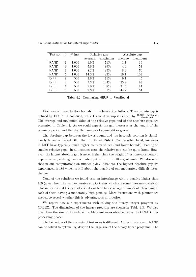
4.6. Computations for the Interchange Model 117
Test set h # inst. Relative gap Absolute gapaverage. maximum average maximum
RAND 2 1,000 1.9% 71% 1.1 39RAND 3 1,000 5.6% 89% 4.9 54RAND 4 1,000 8.2% 85% 8.9 70RAND 5 1,000 14.3% 82% 19.1 103DIFF 2 500 2.6% 71% 9.1 45DIFF 3 500 7.3% 134% 25.9 93DIFF 4 500 7.0% 108% 31.5 114DIFF 5 500 9.3% 81% 44.7 134
Table 4.2: Comparing HEUR to FlowBound
First we compare the flow bounds to the heuristic solutions. The absolute gap is
defined by HEUR − FlowBound, while the relative gap is defined by HEUR−FlowBound
FlowBound.
The average and maximum value of the relative gaps and of the absolute gaps are
presented in Table 4.2. As we could expect, the gap increases as the length of the
planning period and thereby the number of commodities grows.
The absolute gap between the lower bound and the heuristic solution is signifi-
cantly larger in the set DIFF than in the set RAND. On the other hand, instances
in DIFF have typically much higher solution values (and lower bounds), leading to
smaller relative gaps. In all instance sets, the relative gap can be quite large. How-
ever, the largest absolute gap is never higher than the weight of just one considerably
expensive arc, although we computed paths for up to 10 urgent units. We also note
that in our computations on further 5-day instances, the highest absolute gap we
experienced is 189 which is still about the penalty of one moderately difficult inter-
change.
None of the solutions we found uses an interchange with a penalty higher than
109 (apart from the very expensive empty trains which are sometimes unavoidable).
This indicates that the heuristic solutions tend to use a larger number of interchanges,
each of them having a moderately high penalty. More discussions with planner are
needed to reveal whether this is advantageous in practise.
We report now our experiments with solving the binary integer program by
CPLEX. The dimensions of the integer program are shown in Table 4.3. We also
give there the size of the reduced problem instances obtained after the CPLEX pre-
processing phase.
The behaviour of the two sets of instances is different. All test instances in RAND
can be solved to optimality, despite the large size of the binary linear programs. The
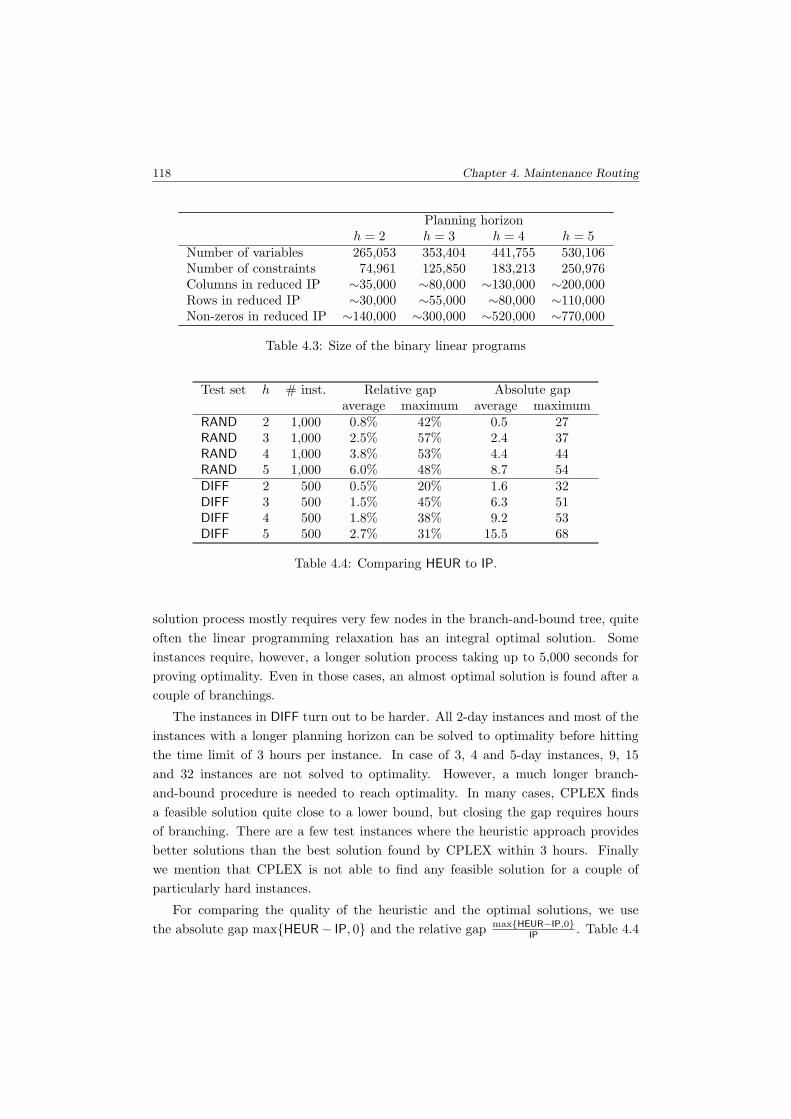
118 Chapter 4. Maintenance Routing
Planning horizonh = 2 h = 3 h = 4 h = 5
Number of variables 265,053 353,404 441,755 530,106Number of constraints 74,961 125,850 183,213 250,976Columns in reduced IP ∼35,000 ∼80,000 ∼130,000 ∼200,000Rows in reduced IP ∼30,000 ∼55,000 ∼80,000 ∼110,000Non-zeros in reduced IP ∼140,000 ∼300,000 ∼520,000 ∼770,000
Table 4.3: Size of the binary linear programs
Test set h # inst. Relative gap Absolute gapaverage maximum average maximum
RAND 2 1,000 0.8% 42% 0.5 27RAND 3 1,000 2.5% 57% 2.4 37RAND 4 1,000 3.8% 53% 4.4 44RAND 5 1,000 6.0% 48% 8.7 54DIFF 2 500 0.5% 20% 1.6 32DIFF 3 500 1.5% 45% 6.3 51DIFF 4 500 1.8% 38% 9.2 53DIFF 5 500 2.7% 31% 15.5 68
Table 4.4: Comparing HEUR to IP.
solution process mostly requires very few nodes in the branch-and-bound tree, quite
often the linear programming relaxation has an integral optimal solution. Some
instances require, however, a longer solution process taking up to 5,000 seconds for
proving optimality. Even in those cases, an almost optimal solution is found after a
couple of branchings.
The instances in DIFF turn out to be harder. All 2-day instances and most of the
instances with a longer planning horizon can be solved to optimality before hitting
the time limit of 3 hours per instance. In case of 3, 4 and 5-day instances, 9, 15
and 32 instances are not solved to optimality. However, a much longer branch-
and-bound procedure is needed to reach optimality. In many cases, CPLEX finds
a feasible solution quite close to a lower bound, but closing the gap requires hours
of branching. There are a few test instances where the heuristic approach provides
better solutions than the best solution found by CPLEX within 3 hours. Finally
we mention that CPLEX is not able to find any feasible solution for a couple of
particularly hard instances.
For comparing the quality of the heuristic and the optimal solutions, we use
the absolute gap max{HEUR − IP, 0} and the relative gap max{HEUR−IP,0}IP
. Table 4.4

4.6. Computations for the Interchange Model 119
Test set h # inst. Relative gap Absolute gapaverage maximum average maximum
RAND 2 1,000 0.8% 30% 0.6 39RAND 3 1,000 2.4% 40% 2.6 39RAND 4 1,000 3.5% 36% 4.5 44RAND 5 1,000 6.6% 36% 10.4 55DIFF 2 500 1.8% 40% 7.5 43DIFF 3 500 4.2% 54% 19.6 80DIFF 4 500 4.0% 49% 22.3 80DIFF 5 500 5.2% 39% 29.2 83
Table 4.5: Comparing FlowBound to IP.
Test set and algorithm h = 2 h = 3 h = 4 h = 5RAND, DIFF FlowBound 1–4 1–5 1–5 2-6RAND, DIFF HEUR 2–4 5–6 7–10 15–18
RAND IP 16–107 58–1,969 222–1,389 734–5006RAND IP (average) 20.4 87.4 297.0 1,054.6DIFF IP 22–616 83–10,800 278–10,800 845–10,800DIFF IP (average) 42.9 352.1 1,170.4 2,507.4
Table 4.6: Running times (in seconds).
shows the average and maximum values of these performance indicators. The quality
of the flow bounds is examined in Table 4.5, the measures are the absolute gap
IP − FlowBound and the relative gap IP−FlowBound
IP. It turns out that the average and
maximum gaps between IP and FlowBound are larger than between HEUR and IP.
This shows that the quality of the heuristic solutions is significantly better than what
the easy-to-compute FlowBound indicates.
Table 4.6 shows the running times for computing the flow bounds, for the heuristic
algorithm and for solving the binary linear programs by CPLEX. We also give the
average running times for the CPLEX computations. We can see that instances in
DIFF require 2 to 4 times longer computation times than instances in RAND.
4.6.4 Conclusions for the Interchange Model
The heuristic solution method solves all test instances, the objective difference be-
tween the heuristic solution and the optimal integral solution is not large in the
weight structure of the instances. This can be explained by the structure of the
problem. The number of urgent units is small compared to the total number of units
120 Chapter 4. Maintenance Routing
(especially in the case of a shorter planning horizon, such as 2 or 3 days), so the
urgent units do not have too much interaction with each other. Also, the timetable
allows enough interchanging possibilities to provide several almost optimal paths for
the urgent units.
In the solutions of the Interchange Model, the only highly penalised interchanges
are empty trains on the first day of the planning horizon for units with a deadline of
24 hours. This indicates that, when solving a sequence of problems every day and
using each day’s output as input for the next day, the system would very rarely use
expensive arcs. However, disturbances and delays may prevent the local shunting
crew to carry out the desired interchanges. This may lead in practise to using more
expensive interchanges, including empty trains.
Despite the large size of the binary integer program, the average solution times
of CPLEX are acceptable, especially for the practically important planning horizons
of 2 and 3 days. For longer periods (but also for some 2 and 3 days instances) the
running times are still a bit longer than convenient in an interactive decision support
application.
The heuristic algorithm we propose is able to solve all test instances. However,
it might not find a feasible solution with other data. In such a case, we may give
up the heuristic approach and just run CPLEX. As an alternative, HEUR (or any
other heuristic algorithm) can be used in an interactive manner. When the heuristic
displays a solution for a subset of urgent units, the maintenance routing planner can
see the conflicts between this partial solution and some candidate paths for urgent
units that have not been routed yet. Then the planner can forbid or enforce some
interchanges and run the heuristic algorithm again. Since the heuristic is fast, the
planner can examine several alternatives within minutes. By storing the planner’s
preferences and using these in later runs, the model may ‘learn’ from the planners.
4.7 The Transition Model
In the previous section we described the Interchange Model for maintenance routing.
Despite promising computational results, the model also has a drawback: It requires
too many details about the shunting possibilities; more than is likely to be available
in practise. Therefore, we present in this section the alternative ‘Transition Model’
which needs less input data. While the Interchange Model tries to reflect the shunt-
ing process as accurately as possible, the Transition Model takes very few details
explicitly into account.

4.7. The Transition Model 121
The Transition Model incorporates no other information on shunting possibilities
than a description of which new transitions are allowed. The sole criterion for that is
whether there is enough time to carry out the shunting operations involved with the
particular transition without causing delays. We assign a weight to every allowed new
transition and define the weight of a solution as a simple function of the weights of
the new transitions in the solution. Since the Transition Model is less involved than
the Interchange Model, it may produce less acceptable solutions. On the other hand,
its input data are a lot easier to obtain and in the setting of an interactive decision
support system the weight function can be tuned based on rejections or approvals of
local shunting crew. In any case, the real strength or weakness of the model can only
be evaluated by implementing it for real-life instances.
The Transition Model itself is a variant of the multi-depot vehicle routing problem,
studied in detail by Desrosiers et al. (1995) and Toth and Vigo (2002). Our results
and methods are related to those by Carraresi and Gallo (1984) and by Bertossi et al.
(1987).
4.7.1 Maintenance Routing Graphs
A regular transition is a pair of tasks that are planned to be carried out by a unit
consecutively in the regular plan. Regular transitions (t, σ (t)) satisfy
sa (t) = sd (σ (t)) ,
τa (t) < τd (σ (t)) .
A candidate transition is a pair of tasks (t, t′) such that it is not a regular transition
and such that
sa (t) = sd (t′) ,
τa (t) 6 τd (t′) − %.
A candidate transition can be interpreted as a pair of an arriving and a departing
event at the same station with a time difference of at least % minutes. It represents
the possibility to join the tasks to duties in another way than the regular plan. The
buffer time % reserves time for possibly needed extra shunting operations, moreover,
it protects against spreading of delays. We assume that the first tasks in the regular
duties have no in-coming candidate transition and the last tasks of the regular duties
have no out-going candidate transition. Regular and candidate transitions together
are called transitions.
122 Chapter 4. Maintenance Routing
The set of tasks together with the set of transitions forms an acyclic graph. Any
directed graph that can be obtained in this way is called a maintenance routing graph
(or MR-graph). Note that MR-graphs are always acyclic.
In a directed graph, a sink is a node without in-coming arcs and a source is a
node without out-going arcs. The set of sources is denoted by V0 and the set of sinks
by V∞. In an MR-graph, the first tasks in the regular duties are the sources, while
the last tasks in the regular duties are the sinks.
Let M be the set of maintenance nodes. The urgencies in an MR-graph G =
(V,A) are given by a set U of sources in G and by sets Mu ⊆ M for each u ∈ U .
Members of U are urgent nodes. In a maintenance routing application, maintenance
nodes are the maintenance tasks. Furthermore, a node is urgent if it is the earliest
task of one of the units that must reach a maintenance facility in the planning period.
For u ∈ U , Mu is the set of maintenance tasks that can be assigned to u in order to
satisfy the maintenance requirement of the corresponding unit.
In real-world maintenance routing, we may allow the buffer time to vary from arc
to arc, but here, an MR-graph always has a uniform buffer time. It also happens
in real world maintenance routing that some practical instances can only be solved
when allowing empty trains. If desired, we can model such movements by transitions
between tasks that arrive and depart at different stations. However, such more
general transitions are not part of the definition of MR-graphs.
4.7.2 Model Formulation
From the timetable and the buffer time %, we construct the corresponding MR-graph.
The sequences of tasks that can be assigned to a single unit over a whole planning
period are precisely the directed paths in the corresponding MR-graph that connect
a source to a sink. A path cover in an acyclic directed graph G = (V,A) is a set of
arcs that forms a collection of node disjoint paths such that the paths cover V and
that each path connects a source of G with a sink of G. The regular transitions in a
maintenance routing graph form a path cover. So, the maintenance routing problem
amounts to finding a path cover such that the path in the path cover that starts at
urgent node u contains a node in Mu.
In order to evaluate shunting efforts, each transition a has a weight, denoted by
c(a); this weight estimates how difficult it is to use for a unit. In Section 4.7.7,
we discuss briefly how we obtain these weights. We measure the overall shunting
difficulty of a solution by the sum of the individual transition weights.

4.7. The Transition Model 123
With these data, the maintenance routing problem becomes the following integer
multi-commodity flow model; we define it for general acyclic graphs for later reference.
Transition Model: Given an acyclic graph G = (V,A), a set U of sources and the
urgencies (Mu : u ∈ U), as well as a weight function c : A → R+, find a path
cover Z minimising
∑
a∈Z
c(a)
such that for each u ∈ U , the path starting at u contains a member of Mu.
We formulate this as a binary linear program. The variables are:
z : A → {0, 1},
xu : A → {0, 1} u ∈ U.
The function z is a network flow where the arcs with z(a) = 1 form a path cover,
that is, the paths of all units during the entire planning period. The functions xu
are also network flows where the arcs with xu(a) = 1 form the path of urgent node
u to a maintenance node. An urgent node u ∈ U is a source while members of Mu
are sinks with respect to the network flow xu.
The integer program reads as follows.
Minimise∑
a∈A
c(a) · z(a) (4.29)
subject to
∑
a∈δin(v)
z(a) = 1 ∀v ∈ V \ V0 (4.30)
∑
a∈δout(v)
z(a) = 1 ∀v ∈ V \ V∞ (4.31)
∑
a∈δin(v)
xu(a) =∑
a∈δout(v)
xu(a) ∀u ∈ U, v ∈ V \ ({u} ∪ Mu) (4.32)
∑
a∈δout(u)
xu(a) = 1 ∀u ∈ U (4.33)
∑
u∈U
∑
a∈δout(v)
xu(a) = 0 ∀v ∈ M (4.34)
124 Chapter 4. Maintenance Routing
∑
u∈U :v/∈M(u)
∑
a∈δin(v)
xu(a) = 0 ∀v ∈ M (4.35)
∑
u∈U
xu(a) 6 z(a) ∀a ∈ A (4.36)
z ∈ {0, 1}A (4.37)
xu ∈ {0, 1}A ∀u ∈ U (4.38)
Constraints (4.30) – (4.31) state that z is a network flow, having a unit throughput
through each node. Constraints (4.32) describe flow conservation for each flow xu.
Constraints (4.33) set the sources of the flows xu. Constraints (4.34) – (4.35) express
that a maintenance node has no out-going flow in any of the flows xu and that it only
accepts in-going flow from an urgent node u if it can be assigned to u. Constraints
(4.36) make sure that the paths indicated by xu are parts of the path cover z. Finally,
constraints (4.37) – (4.38) specify the domain of the variables.
When comparing the Transition Model to the Interchange Model, the most im-
portant difference between both approaches is the collection of constraints in (4.12):
they describe the interaction between units. In reality (and also in the Interchange
Model), a candidate transition may only be cheap because some other candidate
transitions are carried out at the same time. The Transition Model cannot see any
connection between the transitions, therefore it may underestimate the real shunting
difficulty. It will be interesting to see whether or not the Transition Model provides
unrealistic solutions.
4.7.3 Objective Function
As mentioned in Section 4.3, the objective criteria in the maintenance routing prob-
lem are quite vaguely formulated. Therefore, several different objective functions
could be used. We choose (4.29) because it is probably the most simple and intuitive
objective function. However, one can also use
Minimise∑
a∈A
c(a) ·
(∑
u∈U
xu(a)
). (4.39)
In that case, only the urgent units contribute to the total weight of the solution.
In order to make the objective function (4.39) realistic, the weight of a candidate
transition a should reflect the shunting difficulty of those candidate transitions which
arise in the path cover as consequences of a. It is, however, hopeless to incorporate the
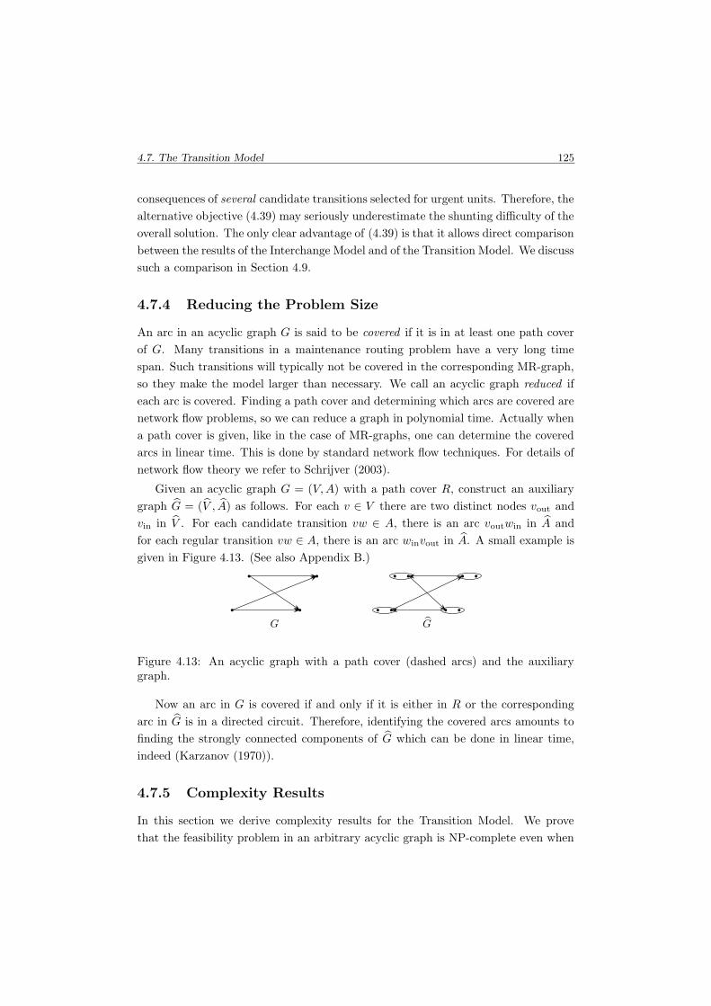
4.7. The Transition Model 125
consequences of several candidate transitions selected for urgent units. Therefore, the
alternative objective (4.39) may seriously underestimate the shunting difficulty of the
overall solution. The only clear advantage of (4.39) is that it allows direct comparison
between the results of the Interchange Model and of the Transition Model. We discuss
such a comparison in Section 4.9.
4.7.4 Reducing the Problem Size
An arc in an acyclic graph G is said to be covered if it is in at least one path cover
of G. Many transitions in a maintenance routing problem have a very long time
span. Such transitions will typically not be covered in the corresponding MR-graph,
so they make the model larger than necessary. We call an acyclic graph reduced if
each arc is covered. Finding a path cover and determining which arcs are covered are
network flow problems, so we can reduce a graph in polynomial time. Actually when
a path cover is given, like in the case of MR-graphs, one can determine the covered
arcs in linear time. This is done by standard network flow techniques. For details of
network flow theory we refer to Schrijver (2003).
Given an acyclic graph G = (V,A) with a path cover R, construct an auxiliary
graph G = (V , A) as follows. For each v ∈ V there are two distinct nodes vout and
vin in V . For each candidate transition vw ∈ A, there is an arc voutwin in A and
for each regular transition vw ∈ A, there is an arc winvout in A. A small example is
given in Figure 4.13. (See also Appendix B.)
G bG
Figure 4.13: An acyclic graph with a path cover (dashed arcs) and the auxiliarygraph.
Now an arc in G is covered if and only if it is either in R or the corresponding
arc in G is in a directed circuit. Therefore, identifying the covered arcs amounts to
finding the strongly connected components of G which can be done in linear time,
indeed (Karzanov (1970)).
4.7.5 Complexity Results
In this section we derive complexity results for the Transition Model. We prove
that the feasibility problem in an arbitrary acyclic graph is NP-complete even when

126 Chapter 4. Maintenance Routing
there is only a single urgent node. When the number of sources is fixed, however,
an optimal solution of the Transition Model can be found in polynomial time with
dynamic programming irrespective the number of urgent nodes. For MR-graphs with
one urgent node, the feasibility version is polynomially solvable, but the optimisation
problem remains NP-hard. The following table summarises these results of this
section.
Complexity of the Transition Model Feasibility Optimising
Arbitrary acyclic graphs, |U | = 1 NP-hard NP-hard
Arbitrary acyclic graphs, fixed number of sources P P
MR-graphs, |U | = 1 P NP-hard
NP-Hardness in Arbitrary Acyclic Graphs
Theorem 4.9. It is NP-complete to decide if an acyclic graph has a path cover such
that one of its paths connects a given source with a given sink.
Proof. We reduce the satisfiability problem to the feasibility of the Transition Model.
Let x1, . . . , xn be Boolean variables, let ε ∈ {+1,−1} and denote
xεj =
{xj if ε = +1,
¬xj if ε = −1.
Consider the conjunctive normal form
ϕ =k∧
i=1
(x
εi1i1
∨ xεi2i2
∨ · · · ∨ xεim(i)
im(i)
).
It is well-known that it is NP-complete to decide whether or not we can assign values
to the variables that make ϕ true (Cook, 1971).
We start with an empty graph. Insert two nodes aj , bj for each variable xj and
draw an arc ajbj . For each i = 0, . . . , k, create three nodes si, ci, di and insert the
arcs cisi, sidi and cidi. Moreover, insert the arc ckd0. Let s = c0 and t = dk.
For the occurrence of a variable xj (either as xj or as ¬xj) in clause i, create a
‘box’ as shown in Figure 4.14. Create 8 new nodes u, v, w, z, g, h, p, q and draw the
arcs uv, uz, wz, gu, hw, vp, zq, gp and gq. Insert the arc si−1u. Moreover, draw the
arc vsi if the non-negated xj occurs in clause i and draw the arc zsi if ¬xj occurs in
clause i.
Order the occurrences of xj by increasing clause index. Draw an arc from aj to
the v-node of the first xj-box. Insert an arc from the w-node of any xj-box to the
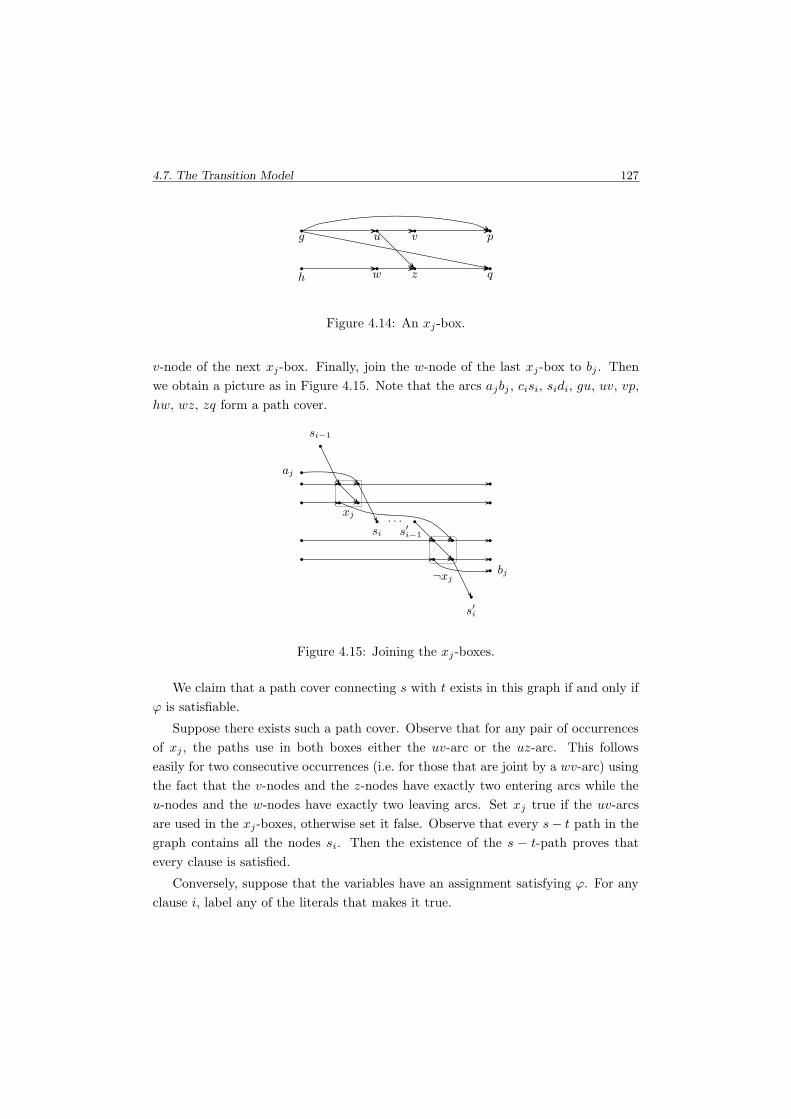
4.7. The Transition Model 127
g u v p
h w z q
Figure 4.14: An xj-box.
v-node of the next xj-box. Finally, join the w-node of the last xj-box to bj . Then
we obtain a picture as in Figure 4.15. Note that the arcs ajbj , cisi, sidi, gu, uv, vp,
hw, wz, zq form a path cover.
. . .
aj
bj
si−1
s′i
si s′i−1
xj
¬xj
Figure 4.15: Joining the xj-boxes.
We claim that a path cover connecting s with t exists in this graph if and only if
ϕ is satisfiable.
Suppose there exists such a path cover. Observe that for any pair of occurrences
of xj , the paths use in both boxes either the uv-arc or the uz-arc. This follows
easily for two consecutive occurrences (i.e. for those that are joint by a wv-arc) using
the fact that the v-nodes and the z-nodes have exactly two entering arcs while the
u-nodes and the w-nodes have exactly two leaving arcs. Set xj true if the uv-arcs
are used in the xj-boxes, otherwise set it false. Observe that every s − t path in the
graph contains all the nodes si. Then the existence of the s − t-path proves that
every clause is satisfied.
Conversely, suppose that the variables have an assignment satisfying ϕ. For any
clause i, label any of the literals that makes it true.
128 Chapter 4. Maintenance Routing
If xj has value true, select the arc ajbj , as well as the uv, wz, hw and zq arcs of
all the xj-boxes. If an occurrence of xj is labelled for clause i, select the si−1u, vsi
and gp-arcs of this box, otherwise select the gu and vp-arcs.
If xj has value false, select the uz, hw and vp-arcs of the xj-boxes, the wv-arcs
between the xj-boxes as well as the arcs connecting the nodes aj and bj to the xj-
boxes. If the occurrence is labelled for clause i, select the arcs si−1u, zsi and gq in
this xj-box, otherwise select the arcs gu and zq.
Finally, select the arcs cidi for i = 1, . . . , k−1 and the arc ckd0. Then the selected
arcs form a path cover connecting s with t. �
Bounded Number of Units
In railway applications, the number of sources equals the number of available rolling
stock units. Maintenance routing instances often share this number, the length of
the planning horizon (and thereby the number of tasks) is the varying parameter.
Then the question arises what can be said about the complexity of the Transition
Model if the number of source nodes in the acyclic graph is constant. The following
theorem implies that the Transition Model with a constant number of source nodes
is solvable in polynomial time.
Theorem 4.10. For any acyclic graph G = (V,A), the optimisation problem (4.29)
– (4.38) can be solved in O((|V ||A|)O(d)
)time where d is the number of sources.
Proof. Let n = |V |, m = |A| and let k = |U |. We assume that the sources are
S = {1, . . . , d} and that U = {1, . . . , k}. The optimisation problem can be reduced
to a shortest path problem in an acyclic graph G′ = (V ′, A′) with at most (2mn)d
nodes and at most (2mn)2d arcs. The sketch of the construction is as follows.
We colour the nodes of G red. By subdividing arcs, we can transform G into a
graph where the node set is partitioned into disjoint subsets W0, . . . ,W` such that
each arc connects Wi to Wi+1 for some index i. We may also assume that the arcs
between W0 and W1 form a matching of size d. The enlarged graph has at most mn
nodes and at most mn arcs. We colour the newly created nodes black. Then a path
cover in the original graph corresponds to a system of paths in the enlarged graph
covering all the red nodes.
Now we construct G′ = (V ′, A′). Create a member of V ′ for every (d + k)-tuple
v′ = (a1, . . . , ad, ε1, . . . , εk) where a1, . . . , ad are arcs connecting subsets Wt−1 and Wt
for some index t such that these arcs cover all the red nodes in Wt−1∪Wt, and where
εj ∈ {0, 1} for each j = 1, . . . , k. The arcs ai indicate the routes of the units through

4.7. The Transition Model 129
the network, while εj encodes whether urgent unit j has undergone maintenance so
far.
Let s′ be the node in V ′ with arcs ai between W0 and W1 and with ε1 = · · · =
εk = 0. Let T ′ contain all nodes v′ ∈ V ′ such that the arcs ai in v′ lie between the
subsets W`−1 and W` and such that εj = 1 for each j.
Let v′ = (a1, . . . , ad, ε1, . . . , εk) and w′ = (b1, . . . , bd, ζ1, . . . , ζk) nodes of G′. Then
(v′, w′) is an arc in G′ if
• for every i, the head of arc ai is the tail of arc bi;
• the paths (ai, bi) for i = 1, . . . , d are node disjoint;
• for every j = 1, . . . , k, ζj = 1 if and only if εj = 1 or if the head of arc bj is an
allowed maintenance node for urgent unit j.
We define the weight of the arc (v′, w′) as∑d
i=1 c(bi).
Then a system of d disjoint paths in G covering all the red nodes and satisfying
all the maintenance requirements corresponds to an s′−T ′-path in G′ with the same
weight and vice versa. �
4.7.6 MR-Graphs with One Urgent Unit
We have seen in the previous section that the feasibility problem with a single urgent
node is NP-complete in general acyclic graphs. It is, however, polynomially solvable
in MR-graphs.
Theorem 4.11. Let G = (V,A) be an MR-graph and let A0 be the set of covered
arcs. Moreover, let s, t ∈ V and suppose that P is an s− t-path in G0 = (V,A0) with
inclusion-wise minimal node set. Then there exists a path cover containing P .
Proof. Let R denote the set of regular transitions. Consider the auxiliary graph G of
G as defined in Section 4.7.2. Let W be the set of nodes vout with v in P and v 6= t.
Let WN be the set of nodes vout ∈ W with vw ∈ P \ R.
We show that no pair of different nodes vout ∈ WN and v′out ∈ W lie in the same
strong component of G.
Suppose the contrary. Let vw and v′w′ be arcs in the path P . We may assume
that v′ lies on P between v and t, the other case being analogous. Let K be the
strong component of G that contains vout and v′out. Then win ∈ K since voutwin
belongs to a directed circuit in G. Moreover, if v′w′ is a regular transition, then
every vout − v′out-path contains the node w′
in since w′inv′
out is the only arc that enters

130 Chapter 4. Maintenance Routing
v′out. If, however, v′w′ is a candidate transition, then v′
outw′in is contained in a circuit
of G. In both cases we have w′in ∈ K. In particular, G contains a w′
in − vout-path P .
For every arc xoutyin ∈ A, we have sa (x) = sd (y) and for every arc xinyout ∈ A,
we have sd (x) = sa (y). Therefore sa (v) = sd (w′). Moreover,
τa (v) 6 τd (w) − % 6 τd (w′) − %.
Thus vw′ is either a regular transition (and thus it is covered) or a candidate tran-
sition. In the latter case, P ∪ {voutw′in} is a circuit in G. Therefore vw′ is covered.
This contradicts the minimality of the path P . Therefore vout and v′out cannot lie in
the same strong component of G.
For every arc vw ∈ P \ R, fix a directed circuit Cv,w in G containing the arc
voutwin. Let C be the set of those edges in G that correspond in G to an edge in⋃{Cv,w : vw ∈ P \ R}. Then the circuits Cv,w are node disjoint, therefore (R \C)∪
(C \ R) is a path cover of G. Moreover, no arc in P ∩ R belongs to C, therefore
(R \ C) ∪ (C \ R) contains P . �
This implies
Corollary 4.12. The feasibility problem of the Transition Model in an MR-graph
with one urgent node can be solved in polynomial time.
The NP-hardness of the feasibility problem in arbitrary acyclic graphs is partly
caused by sparsity of some acyclic graphs that are not MR-graphs. The proof above
is based on the property of MR-graphs that the existence of a certain pair of arcs vw
and v′w′ implies the existence of the arc vw′.
Theorem 4.11 requires that the node set of path P is inclusion-wise minimal. One
may ask whether each directed s − t-path in an MR-graph extends to a path cover.
Figure 4.16 shows an example that this is not so: the path formed by the bold arcs
cannot be extended to a path cover.
The algorithm for the feasibility problem does not extend to the optimisation
version of the single urgent unit case. Reason is that the weight of a path serving the
urgent unit does not reflect the weight of a corresponding solution, as also non-urgent
units will use new transitions and these do contribute to the weight of the solution as
well. Actually, finding an optimal solution of the Transition Model with one urgent
node is also NP-hard in MR-graphs.
Theorem 4.13. It is NP-hard to find an optimal solution of the transition model
on MR-graphs with one urgent unit, one maintenance task and {0, 1}-valued weight
function.
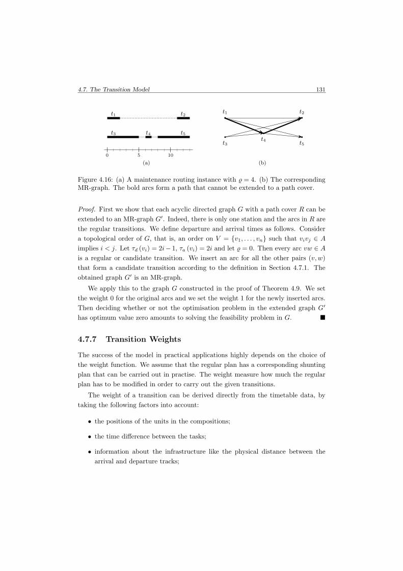
4.7. The Transition Model 131
0 5 10
t1 t2
t3 t4 t5
(a)
t1 t2
t3t4
t5
(b)
Figure 4.16: (a) A maintenance routing instance with % = 4. (b) The correspondingMR-graph. The bold arcs form a path that cannot be extended to a path cover.
Proof. First we show that each acyclic directed graph G with a path cover R can be
extended to an MR-graph G′. Indeed, there is only one station and the arcs in R are
the regular transitions. We define departure and arrival times as follows. Consider
a topological order of G, that is, an order on V = {v1, . . . , vn} such that vivj ∈ A
implies i < j. Let τd (vi) = 2i− 1, τa (vi) = 2i and let % = 0. Then every arc vw ∈ A
is a regular or candidate transition. We insert an arc for all the other pairs (v, w)
that form a candidate transition according to the definition in Section 4.7.1. The
obtained graph G′ is an MR-graph.
We apply this to the graph G constructed in the proof of Theorem 4.9. We set
the weight 0 for the original arcs and we set the weight 1 for the newly inserted arcs.
Then deciding whether or not the optimisation problem in the extended graph G′
has optimum value zero amounts to solving the feasibility problem in G. �
4.7.7 Transition Weights
The success of the model in practical applications highly depends on the choice of
the weight function. We assume that the regular plan has a corresponding shunting
plan that can be carried out in practise. The weight measure how much the regular
plan has to be modified in order to carry out the given transitions.
The weight of a transition can be derived directly from the timetable data, by
taking the following factors into account:
• the positions of the units in the compositions;
• the time difference between the tasks;
• information about the infrastructure like the physical distance between the
arrival and departure tracks;

132 Chapter 4. Maintenance Routing
Planning period 2 days 3 days 4 days 5 days# of tasks 1,196 1,762 2,326 2,709# of transitions 98,035 198,614 332,031 508,853# of covered transitions 11,394 17,067 22,830 28,570
Table 4.7: Dimensions of the graph model.
• the station where the transition takes place; stations with heavy traffic provide
less changing possibilities;
• the time that the transition is carried out; changes during rush hours are hard,
while changes at night are typically easy.
In our implementations, we followed another method: We used the Interchange
Model as a detailed model of the shunting possibilities to compute the weights. We
did so in order to be able to compare the output of both models on the same input.
We shall explain more details about this in Section 4.9. Note again that whichever
method is used to determine the transition weights, the values can be updated when
the model is applied for solving real-life problems.
4.8 Computations for the Transition Model
As for the Interchange Model, we use the units of the type “Sprinter” as test example:
we consider the same set of tasks. Recall that there are two maintenance tasks on
every day. For simplicity, we set the buffer time % uniformly to 10 minutes based on
discussions with the planners.
For the computations we used the modelling software ILOG OPL Studio 3.7 and
the integer program solver ILOG CPLEX 9.0 on a PC with an Intel P4 3.0 GHz
processor and 512 Mb internal memory.
When generating the candidate transitions, the graph turns out to be quite large
(see Table 4.7). However, the reduction step described in Section 4.7.4 results in
decreasing the number of arcs dramatically. Without this reduction, the binary
linear programs would become far too large for acceptable computation times.
We consider planning horizons of 2 up to 5 days. Since the maintenance tasks
start at the same time at the same location on every day, the integer program requires
only one flow xu for every possible deadline. The dimensions of the integer programs
are given in Table 4.8. We solve the sets RAND and DIFF of instances that we
described in Section 4.6.2.
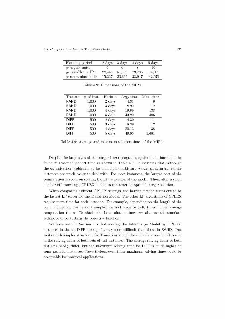
4.8. Computations for the Transition Model 133
Planning period 2 days 3 days 4 days 5 days# urgent units 4 6 8 10# variables in IP 28,453 51,193 79,786 114,096# constraints in IP 15,337 23,816 32,947 42,672
Table 4.8: Dimensions of the MIP’s.
Test set # of inst. Horizon Avg. time Max. timeRAND 1,000 2 days 4.31 6RAND 1,000 3 days 8.92 12RAND 1,000 4 days 19.69 138RAND 1,000 5 days 43.20 486DIFF 500 2 days 4.30 11DIFF 500 3 days 8.39 12DIFF 500 4 days 20.13 138DIFF 500 5 days 49.03 1,681
Table 4.9: Average and maximum solution times of the MIP’s.
Despite the large sizes of the integer linear programs, optimal solutions could be
found in reasonably short time as shown in Table 4.9. It indicates that, although
the optimisation problem may be difficult for arbitrary weight structures, real-life
instances are much easier to deal with. For most instances, the largest part of the
computation is spent on solving the LP relaxation of the model. Then, after a small
number of branchings, CPLEX is able to construct an optimal integer solution.
When comparing different CPLEX settings, the barrier method turns out to be
the fastest LP solver for the Transition Model. The other LP algorithms of CPLEX
require more time for each instance. For example, depending on the length of the
planning period, the network simplex method leads to 3–10 times higher average
computation times. To obtain the best solution times, we also use the standard
technique of perturbing the objective function.
We have seen in Section 4.6 that solving the Interchange Model by CPLEX,
instances in the set DIFF are significantly more difficult than those in RAND. Due
to its much simpler structure, the Transition Model does not show sharp differences
in the solving times of both sets of test instances. The average solving times of both
test sets hardly differ, but the maximum solving time for DIFF is much higher on
some peculiar instances. Nevertheless, even those maximum solving times could be
acceptable for practical applications.
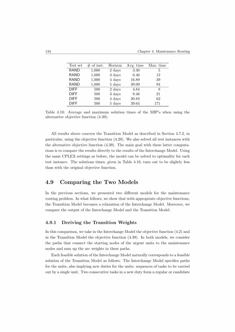
134 Chapter 4. Maintenance Routing
Test set # of inst. Horizon Avg. time Max. timeRAND 1,000 2 days 3.30 5RAND 1,000 3 days 6.46 12RAND 1,000 4 days 16.89 39RAND 1,000 5 days 39.09 94DIFF 500 2 days 4.84 8DIFF 500 3 days 9.46 21DIFF 500 4 days 20.83 62DIFF 500 5 days 39.64 171
Table 4.10: Average and maximum solution times of the MIP’s when using thealternative objective function (4.39).
All results above concern the Transition Model as described in Section 4.7.2, in
particular, using the objective function (4.29). We also solved all test instances with
the alternative objective function (4.39). The main goal with these latter computa-
tions is to compare the results directly to the results of the Interchange Model. Using
the same CPLEX settings as before, the model can be solved to optimality for each
test instance. The solutions times, given in Table 4.10, turn out to be slightly less
than with the original objective function.
4.9 Comparing the Two Models
In the previous sections, we presented two different models for the maintenance
routing problem. In what follows, we show that with appropriate objective functions,
the Transition Model becomes a relaxation of the Interchange Model. Moreover, we
compare the output of the Interchange Model and the Transition Model.
4.9.1 Deriving the Transition Weights
In this comparison, we take in the Interchange Model the objective function (4.2) and
in the Transition Model the objective function (4.39). In both models, we consider
the paths that connect the starting nodes of the urgent units to the maintenance
nodes and sum up the arc weights in these paths.
Each feasible solution of the Interchange Model naturally corresponds to a feasible
solution of the Transition Model as follows. The Interchange Model specifies paths
for the units, also implying new duties for the units: sequences of tasks to be carried
out by a single unit. Two consecutive tasks in a new duty form a regular or candidate
4.10. Conclusions 135
transition in the Transition Model; these transitions together give a feasible solution
of the Transition Model.
The only difficulty is to relate the objective functions to each other. The Inter-
change Model works with fine details of the shunting possibilities, therefore it is a
natural idea to derive the transition weights from the Interchange Model. Consider a
transition (t, t′). Then tasks t and t′ are represented in the Interchange Model as task
arcs (v, w) and (v′, w′). Recall that the arc weights in the graph representation of the
Interchange Model are denoted by weight(a). Now we define the weight of transition
(t, t′), denoted by c(t, t′), as the length of the shortest path from w to v′ with respect
to the arc lengths weight(a). With these transition weights, each feasible solution of
the Interchange Model with total weight q corresponds to a feasible solution of the
Transition Model with total weight of at most q. Therefore we have
Theorem 4.14. The Transition Model with the objective function (4.39) and tran-
sition weights c is a relaxation of the Interchange Model.
We point out that deriving the transition weights from the Interchange Model
may not be possible in a real-life application. The main motivation for the Transition
Model is that the vast amount of input data needed for the Interchange Model may
likely be inaccessible.
4.9.2 Numerical Results
Let IM denote the optimal objective value of the Interchange Model and TM the
optimal objective value of the Transition Model. Then the absolute gap is IM − TM
and the relative gap is IM−TM
TM. The average and maximum values of these gaps,
separately computed for the test sets RAND and DIFF, are given in Table 4.11.
It turns out that the objective values of the Transition Model are surprisingly
close to the optimum values of the Interchange Model. In fact, the majority of the
instances in RAND had the same objective value for both models. Instances in the set
DIFF have, as expected, larger differences between the models. However, the largest
absolute difference is again smaller than the weight of a single moderately expensive
arc. The small relative gaps for instances in DIFF are caused by the fact that the
objective values in DIFF are much higher on average than in RAND.
4.10 Conclusions
In this chapter we described the maintenance routing problem of NSR. We presented
two mathematical models for this problem: the Interchange Model and Transition
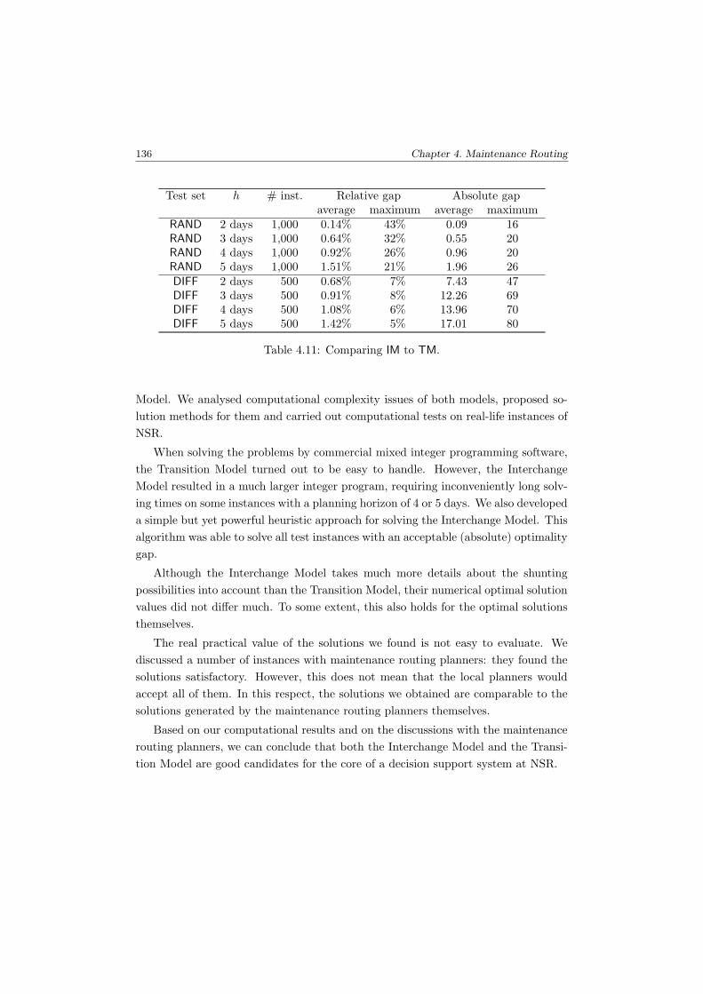
136 Chapter 4. Maintenance Routing
Test set h # inst. Relative gap Absolute gapaverage maximum average maximum
RAND 2 days 1,000 0.14% 43% 0.09 16RAND 3 days 1,000 0.64% 32% 0.55 20RAND 4 days 1,000 0.92% 26% 0.96 20RAND 5 days 1,000 1.51% 21% 1.96 26DIFF 2 days 500 0.68% 7% 7.43 47DIFF 3 days 500 0.91% 8% 12.26 69DIFF 4 days 500 1.08% 6% 13.96 70DIFF 5 days 500 1.42% 5% 17.01 80
Table 4.11: Comparing IM to TM.
Model. We analysed computational complexity issues of both models, proposed so-
lution methods for them and carried out computational tests on real-life instances of
NSR.
When solving the problems by commercial mixed integer programming software,
the Transition Model turned out to be easy to handle. However, the Interchange
Model resulted in a much larger integer program, requiring inconveniently long solv-
ing times on some instances with a planning horizon of 4 or 5 days. We also developed
a simple but yet powerful heuristic approach for solving the Interchange Model. This
algorithm was able to solve all test instances with an acceptable (absolute) optimality
gap.
Although the Interchange Model takes much more details about the shunting
possibilities into account than the Transition Model, their numerical optimal solution
values did not differ much. To some extent, this also holds for the optimal solutions
themselves.
The real practical value of the solutions we found is not easy to evaluate. We
discussed a number of instances with maintenance routing planners: they found the
solutions satisfactory. However, this does not mean that the local planners would
accept all of them. In this respect, the solutions we obtained are comparable to the
solutions generated by the maintenance routing planners themselves.
Based on our computational results and on the discussions with the maintenance
routing planners, we can conclude that both the Interchange Model and the Transi-
tion Model are good candidates for the core of a decision support system at NSR.

Chapter 5
Operational Rolling Stock
Planning
In this chapter we consider the operational rolling stock planning problem of NSR;
the term ‘operational planning’ refers to a planning horizon of 3 days to 2 months. We
describe the operational rolling stock circulation problem and the two-phase method
the planners at NSR use to handle it. In this thesis we only study the second phase in
detail; investigation of the first phase is a subject of further research. We analyse the
complexity of the second phase and propose solution methods for it. We illustrate
the power and the limitations of the methods on instances of NSR.
5.1 Operational Rolling Stock Circulations
In operational planning the tactical rolling stock schedules are adjusted to the partic-
ular weeks. Operational rolling stock planning consists of two tasks: The operational
rolling stock circulations have to be created by the central planners and the corre-
sponding operational shunting plans have to be set up by the local planners. Here
we only deal with the rolling stock circulations.
A general overview of operational planning is given in Section 2.2.4. We mentioned
there that most effort in operational rolling stock planning is spent on large-scale
adjustments of the tactical plans; this is often necessary when parts of the railway
infrastructure become temporarily unavailable. We focus in this chapter on problem
instances of such character.
137

138 Chapter 5. Operational Rolling Stock Planning
Concerning the input, the constraints and the assumptions, the operational rolling
stock circulation problem is similar to its tactical variant. The same assumptions
are made on the shunting process as described in Sections 3.3 and 3.4 for tactical
planning. The available rolling stock has to be assigned to the trips such that the
same constraints are satisfied as in tactical planning. These constraints are listed in
Section 3.5.
The operational plan is not a stand-alone rolling stock plan: It should fit to
the rolling stock circulations before and after the considered planning period. In
particular, the initial inventories (i.e. those at the beginning of the planning period)
must be equal to the number of units that are located at the stations at the beginning
of the planning period. These initial inventories are specified by the rolling stock
schedules that are to be carried out before the planning period; these schedules are
determined in tactical planning or in earlier stages of operational planning. Similar
constraints hold for the final inventories.
It is not always possible to realise all desired inventories. Then the rolling stock
balance must be maintained by sending units from one station to another as empty
trains. Although this is undesirable, it often happens in practise.
Example. Figure 5.1(a) shows the tactical rolling stock circulation
for a small railway network consisting of 8 trips between stations
A, B and C. The grey and black units are of different types. The
desired initial and final inventories are also indicated; the tactical
plan complies with these desired inventories.
Cancelling two trips (indicated by dashed lines) enforces one to mod-
ify the tactical plans. A possible operational rolling stock circulation
is shown in Figure 5.1(b). This operational rolling stock circulation
realises the desired final inventories but there is an off-balance in
the initial inventories: A grey unit is available at station A but the
operational rolling stock circulation requires a black unit. Similarly,
a black unit is available at station B but the operational rolling
stock circulation requires a grey unit.
5.1.1 Differences between Tactical and Operational Planning
The major differences between tactical and operational rolling stock planning are the
planning horizon and the objective criteria. In tactical planning, the rolling stock
is scheduled for the forthcoming two months (at least), the emphasis is on a good
balance of efficiency, service quality and robustness. It takes several weeks until the
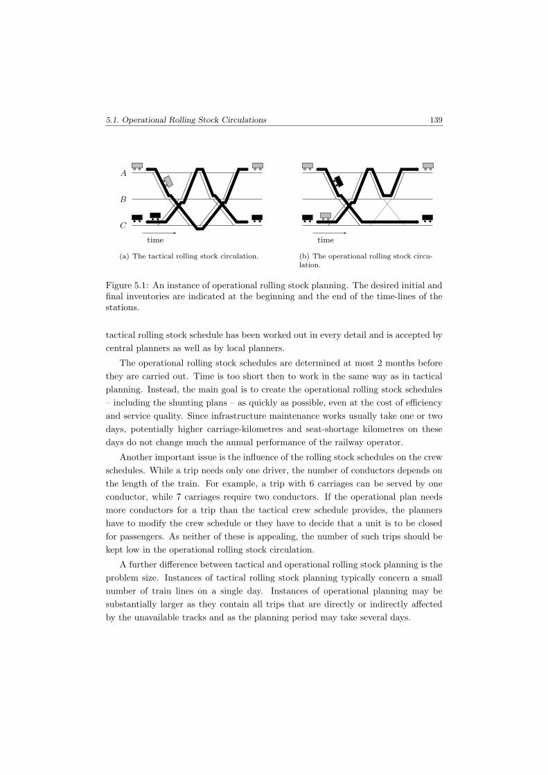
5.1. Operational Rolling Stock Circulations 139
time
A
B
C
(a) The tactical rolling stock circulation.
time
(b) The operational rolling stock circu-lation.
Figure 5.1: An instance of operational rolling stock planning. The desired initial andfinal inventories are indicated at the beginning and the end of the time-lines of thestations.
tactical rolling stock schedule has been worked out in every detail and is accepted by
central planners as well as by local planners.
The operational rolling stock schedules are determined at most 2 months before
they are carried out. Time is too short then to work in the same way as in tactical
planning. Instead, the main goal is to create the operational rolling stock schedules
– including the shunting plans – as quickly as possible, even at the cost of efficiency
and service quality. Since infrastructure maintenance works usually take one or two
days, potentially higher carriage-kilometres and seat-shortage kilometres on these
days do not change much the annual performance of the railway operator.
Another important issue is the influence of the rolling stock schedules on the crew
schedules. While a trip needs only one driver, the number of conductors depends on
the length of the train. For example, a trip with 6 carriages can be served by one
conductor, while 7 carriages require two conductors. If the operational plan needs
more conductors for a trip than the tactical crew schedule provides, the planners
have to modify the crew schedule or they have to decide that a unit is to be closed
for passengers. As neither of these is appealing, the number of such trips should be
kept low in the operational rolling stock circulation.
A further difference between tactical and operational rolling stock planning is the
problem size. Instances of tactical rolling stock planning typically concern a small
number of train lines on a single day. Instances of operational planning may be
substantially larger as they contain all trips that are directly or indirectly affected
by the unavailable tracks and as the planning period may take several days.
140 Chapter 5. Operational Rolling Stock Planning
We note that in practise, rules of operational planning are somewhat less strict
than rules of tactical planning. Getting closer to executing the rolling stock schedules,
there is more space for ad hoc measures to keep the system run smoothly.
5.1.2 Two-phase Approach
Planners at NSR handle the operational rolling stock circulation problem by the
following two-phase method. In the first phase, they try to set up a simple rolling
stock circulation that satisfies as much of the specifications as possible. To that
end, they disregard the constraints on initial inventories and create an intermediate
plan that satisfies all other constraints. This intermediate plan is intended to have
the smallest possible number of composition changes between the trips and their
successors. In practise, the planners often start with specifying the compositions of
the trips at the end of the planning period. They do it in such a way that the numbers
of units per type that end up at the stations are equal to the desired final inventories.
Then they proceed by assigning to any trip the same composition as to its successor.
Roughly speaking, the trains go up and down without any composition change. In
the intermediate plan seat shortages are not minimised explicitly. Nevertheless, the
planners make sure that each trip receives a certain minimal seat capacity which is
often given in the specifications. This may force the planners to allow a small number
of composition changes in the intermediate plan.
The intermediate plan may have a ‘surplus’ or a ‘deficit’ of units at certain stations
at the beginning or the end of the planning period. A station has a deficit in the
initial inventory if the desired initial inventory is smaller than the number of units
that start at that station according to the intermediate plan. A station has a deficit
in the final inventory if the number of units that end up at that station according
to the intermediate plan is smaller than the desired final inventory. Surpluses are
defined analogously: A station has a surplus in the initial inventory if the desired
initial inventory is larger than the number of units that start at that station according
to the intermediate plan. A station has a surplus in the final inventory if the number
of units that end up at that station according to the intermediate plan is larger than
the desired final inventory. Deficits and surpluses are also called off-balances.
Example. Consider again the example in Figure 5.1. The opera-
tional rolling stock circulation has no surplus or deficit in the final
inventories. Station A has a surplus of one grey unit and a deficit of
one black unit, while station C has a surplus of one black unit and
a deficit of one grey unit.

5.1. Operational Rolling Stock Circulations 141
In the second phase, the off-balances are resolved, we call this phase rebalancing.
It amounts to finding a rolling stock circulation where the sum of the surpluses is
as small as possible (zero ideally). Compared to the intermediate plan, the output
rolling stock circulation may not have new surpluses and deficits at any location and
at any time.
Rebalancing is done in practise by simple modifications of the intermediate plan:
(i) adjust the train lengths by coupling or uncoupling units; (ii) assign units of an-
other type to some trips (and all their successors and predecessors); (iii) insert extra
empty trains. The total number of shunting movements is kept low by applying only
a small number of such modifications. This increases the chance that the shunting
planners can create the shunting plans quickly.
Planners prefer operational rolling stock circulations that differ little from the in-
termediate plan in the sense that only few trips are modified in the rebalancing phase.
The reason for this is the fact that the modifications are done manually. Obviously,
this criterion is obsolete in a fully computer-based decision support system.
Note that in most instances, changing the rolling stock types (i.e. option (ii)
above) is undesirable in practise; it is considered to be an ad hoc measure. The
models in this chapter do not include this option.
Both in theory and in practise, an important special case of rebalancing is to
resolve the off-balance of just one unit : a rolling stock circulation has to be modified
so that the inventory at station s1 at time t1 decreases by one, while the inventory
at station s2 at time t2 increases by one. Methods for this can be useful also in
short-term planning to correct off-balances caused by disruptions.
5.1.3 Modelling Approaches
The successful application of the Composition Model in tactical planning (Chapter 4)
suggests that it can also be used in operational planning. Although operational
rolling stock planning is still being done manually at NSR, the Composition Model
is used time to time to set up the intermediate plan. Creating the intermediate
plan manually is very time-consuming for complex instances such as the Noord-Oost
line group; using the Composition Model for this speeds up the planning process.
Note that the model is solved separately for each day of the planning horizon. The
intermediate plan produced by the Composition Model mostly contains some off-
balances. In the rebalancing phase, the planners apply ad hoc methods to resolve
them.
142 Chapter 5. Operational Rolling Stock Planning
Most rolling stock circulation instances of NSR have a simpler structure than the
Noord-Oost line group: splitting and combining of trains does not occur. As reported
in Section 3.11.5, the Composition Model turns out to be solvable on such instances
of tactical planning within a couple of minutes. Yet, it has still to be investigated
whether solving the Composition Model by a commercial MIP solver can cope with
real-life operational planning problems as they may have a much larger size than
tactical planning problems.
In this chapter we look for an alternative approach for solving the operational
rolling stock circulation problem: We try to automate the two-phase solution method
described above, thereby supporting the planning process without changing it sub-
stantially. The emphasis is on finding fast yet reliable heuristic methods. Here we
only consider instances without splitting and combining of trains. Furthermore, dis-
cussions with planners revealed that creating the intermediate plans – even manually
– is pretty straightforward for such instances. Therefore we only study the rebalanc-
ing problem.
5.1.4 Operational Rolling Stock Planning in the Literature
Since operational rolling stock planning is highly reminiscent of tactical planning,
most of the publications listed in Section 3.1 are also relevant to this chapter. We
mention in particular the papers of Ben-Khedher et al. (1998), Lingaya et al. (2002)
and Ziarati et al. (1997): they concern problems whose planning horizon and for-
mulation are closest to those in this chapter. These three papers also deal with
maintenance of the rolling stock but at NSR this is considered only in short-term
planning.
5.2 The Rebalancing Problem
The rebalancing problem is formulated as follows:
Definition 5.1. Rebalancing problem: The input is the timetable and the in-
termediate plan; we assume that trains are not split nor combined. The shunting
assumptions are as described in Sections 3.3 and 3.4. The intermediate plan is a
rolling stock circulation satisfying all constraints in Section 3.5 except those on the
initial and final inventories.
The objective is to find a rolling stock circulation that resolves off-balances with-
out creating new ones such that the weighted sum of the following three quantities

5.3. NP-Completeness of the Rebalancing Problem 143
is minimised: the amount of unresolved off-balances; the number of trips that are
modified during rebalancing; and the number of trips whose train length in the output
exceeds a certain limit (depending on the trip).
In railway practise, minimising the amount of unresolved off-balances is usually
more important than the other two criteria. Note that the third optimisation criterion
aims at minimising the number of trips that require more conductors than in the
tactical plan.
It is worth mentioning that in the case of a single rolling stock type, the re-
balancing problem is a single-commodity flow problem with a non-convex objective
function: it may cost the same to assign two or three units to a trip that is served
by one unit in the intermediate plan. Here we only consider instances with multiple
types.
In what follows, we prove that the feasibility version of the rebalancing problem
is NP-complete, even when resolving an off-balance of just one unit. Then we look
for solution methods.
5.3 NP-Completeness of the Rebalancing Problem
In this section we prove that it is NP-complete to decide whether the rebalancing
problem has a feasible solution even if, with a given integer number k, a single station
has a surplus of k units in the initial inventory and another station has a deficit of
k units in the final inventory. Subsequently, we extend the construction in the proof
and show that the problem remains NP-complete in the case of an off-balance of a
single unit. Before that, we introduce some notations and assumptions and describe
a ‘gadget’ that plays an important role in the NP-completeness proofs.
The instances of the rebalancing problem in this section contain stations with
left-hand shunting side, indicated by [L], and stations with right-hand shunting side,
indicated by [R]. The uncoupling side of each arriving trip is the shunting side of its
arrival station and the coupling side of each departing trip is the shunting side of
its departure station. There are two rolling stock types P and Q. Each trip must
receive one or two units.
In the figures throughout the whole section, the railway networks are drawn in
time-space diagrams: Each station is represented by a horizontal time-line, the time
increases to the right. The trips correspond to diagonal lines between the time-lines.
Train stops are indicated by dots. Dotted arcs between arrival and departure events
connect the trips to their successors.

144 Chapter 5. Operational Rolling Stock Planning
In the figures, some trips have no departure or arrival station. Consider these
stations to be anonymous. All anonymous stations are different. Trips to or from
anonymous stations always have a single unit of a certain type in the intermediate
plan. Anonymous stations with a departing trip always have initial inventory 1 for
this type and 0 for the other type; the final inventory is 0 for both types. The
analogous condition holds for anonymous stations with an arriving trip: the initial
inventories are 0, the final inventory is 1 for the type of the arriving unit and 0 for
the other type.
In the intermediate plan, trips are operated by a single unit of type P (in the
figures below represented by thick solid lines), by a single unit of type Q (thick dotted
lines) or by a two-unit composition PP (thick dashed lines).
5.3.1 Building Blocks for the Proofs: the Gadgets
A gadget is a part of the railway network shown in Figure 5.2. It contains trips
between 8 stations α1, α2, β, γ, δ, ε, ω1 and ω2. Trip s1 from α1 to γ, trip s2 from
α2 to β, trip t1 from ε to ω1 and trip t2 from δ to ω2 (as well as their predecessors
and successors) are each operated in the intermediate plan by a single unit of type
P . The trips from β to γ, from γ to δ and from δ to ε (as well as their predecessors
and successors) are each operated by a single unit of type Q. Stations β and δ allow
shunting on the left hand side only, while stations α1, α2, γ, ε, ω1 and ω2 allow
shunting on the right hand side only.
The initial and final inventories of stations β, γ, δ and ε are 0. Stations α1, α2,
ω1 and ω2 have undefined initial and final inventories in type P and they have zero
initial and final inventory in type Q.
α1 [R]
α2 [R]
β [L]
γ [R]
δ [L]
ε [R]
ω1 [R]
ω2 [R]
s1
s2
t1
t2
Intermediate plan:
P
Q
Figure 5.2: A gadget.

5.3. NP-Completeness of the Rebalancing Problem 145
Lemma 5.2. Consider a rolling stock circulation for a gadget that satisfies the given
inventory, shunting and train length constraints. Then the following holds:
(i) Trip s1 has composition PP if and only if trip t1 has composition PP .
(ii) Trip s2 has composition PP if and only if trip t2 has composition PP .
(iii) At most one of the trips t1 and t2 can have composition PP .
Proof. (i) If trip s1 has composition PP , then a unit can be uncoupled from it at
station γ. This unit can be coupled to the right-hand side of the unit that travels
from γ towards ε. Then the unit of type P can only be uncoupled at station ε.
Actually, this is the only possibility to lead the uncoupled unit to either ω1 or ω2.
Moreover, this is the only way to get composition PP for trip t1.
(ii) Similar to (i).
(iii) Two extra units of type P can reach stations ω1 and ω2 only if the trip between
γ and δ has composition PQP . However, this would violate the upper bound on the
train length. �
We use the simplified symbol in Figure 5.3 for a gadget. The main purpose of a
gadget is to bring an additional unit either from α1 to ω1, or from α2 to ω2, but not
both.
α1
α2
ω1
ω2
s1
s2
t1
t2
Figure 5.3: A simple symbol for a gadget.
5.3.2 Resolving an Off-balance of k Units
Consider an undirected graph G = (V,E) with V = {1, . . . , n} and let k be a positive
integer with k 6 n. We build an instance of the rebalancing problem that is feasible
if and only if G contains a stable set of size k. A stable set is a subset of nodes such
that no pair of them is joined by an edge. It is well known that deciding whether the
graph has a stable set with k nodes is NP-complete (Karp (1972)).
Create two stations A and Z. For every node v ∈ V with dv neighbours, we
create dv + 1 stations Sv1 , . . . , Sv
dv+1. The shunting side of all these stations is the
right-hand side.
146 Chapter 5. Operational Rolling Stock Planning
For each v ∈ V , insert a trip from station A to station Sv1 and insert a trip from
station Svdv+1 to station Z. For each trip from A to a station Sv
1 , create a predecessor
trip from an anonymous station to A. For each trip arriving at Z, insert a successor
from Z to an anonymous station. All trips so far are operated with a single unit of
type P in the intermediate plan.
For each node v ∈ V with neighbours u1, . . . , udv, assign stations Sv
1 , . . . , Svdv
to
the edges u1v, . . . , udvv, bijectively in an arbitrary way. For each edge uv ∈ E with
u < v, add a gadget as follows. Let Sui and Sv
j be the stations assigned to edge uv.
Create four new stations β, γ, δ and ε, set α1 = Sui , α2 = Sv
j , ω1 = Sui+1, ω2 = Sv
j+1
and insert all the trips described in the definition of a gadget. A station Svj with
1 < j < dv +1 belongs to exactly two gadgets and has one arriving and one departing
trip. The departing trip is the successor of the arriving trip.
This completes the railway network. Its size is polynomial in n: it contains O(n2)
trips between O(n2) stations. The network for a small graph is shown schematically
in Figure 5.4.
The intermediate plan satisfies the following inventory constraints. The initial
and final inventories for type Q are 0 (except for some anonymous stations inside the
gadgets). For type P , the initial and final inventories of stations Svj are 0. Station
A has initial and final inventory k, while station Z has initial and final inventory 0.
The initial and final inventories of β-, γ-, δ- and ε-stations of the gadgets are all zero.
The desired inventories differ from these at two points. The desired final inventory
of station A in type P is 0, the desired final inventory of station Z in type P is k. In
some sense, rebalancing means that k units of type P must be routed from A to Z.
Note that the inventory and train length constraints do not leave much choice
for feasible rolling stock circulations. Each trip has either the same composition as
in the intermediate plan or it receives the original composition extended by a single
unit of type P .
Theorem 5.3. Graph G = (V,E) contains a stable set of size k if and only if the
instance of the rebalancing problem constructed above has a feasible solution.
Proof. Suppose that G contains the stable set {v1, . . . , vk}. A solution of the rebal-
ancing problem can be obtained as follows. Couple the k units of type P at station
A to the k trips that depart towards stations Sv11 , . . . , Svk
1 .
Consider any gadget that connects stations Svi
j and Svi
j+1 for some indices i and j.
We adjust the intermediate plan inside the gadget as follows. The trips of this gadget
that are incident to stations Svi
j and Svi
j+1 get composition PP ; we also make all the
necessary modifications to route the additional unit through the gadget from Svi
j to

5.3. NP-Completeness of the Rebalancing Problem 147
v1 v2
v3 v4
G = (V, E) Sv21
Sv11
Sv31
Sv22
Sv41
Sv23
Sv42
Sv24
Sv33
Sv13
Sv12
Sv32
v1 v2 v3 v4
Figure 5.4: An example of the construction of the network.
Svi
j+1. The adjustment of the gadgets can be done simultaneously because there is no
edge between the nodes v1, . . . , vk. Then all the k excess units reach station Z where
they can be uncoupled. Therefore, the rebalancing problem is feasible.
Conversely, consider a solution of the rebalancing problem. At station A, k units
of type P are coupled to trips towards stations, say, Sv11 , . . . , Svk
1 . These units pass
through all gadgets that are related to the nodes v1, . . . , vk and end up at station Z.
Then the nodes v1, . . . , vk form a stable set in G as otherwise Lemma 5.2 (iii) would
be violated. �
Corollary 5.4. The feasibility version of the rebalancing problem is NP-complete in
the case of an off-balance of k units.
5.3.3 Resolving an Off-balance of One Unit
Here we extend the construction described in the previous section. Thereby we prove
that the maximum stable set problem can be reduced to the rebalancing problem with
an off-balance of one unit.
Let G = (V,E) be an undirected graph with |V | = n and let k be a positive integer
with k 6 n. Consider the railway network constructed in the previous section. It is
represented in Figure 5.5 by stations A and Z and the grey box between them.
Create k + 1 new stations α1, . . . , αk and ω. Insert 4k trips as follows (see Fig-
ure 5.5). Create a trip from αi to αi+1 for each i = 1, . . . , k (where αk+1 = ω)
and insert their predecessors and successors from and to anonymous stations. Also
insert a trip that departs from station αi and returns to the same station and has no
predecessor or successor. All these new trips are operated by a single unit of type P
in the intermediate plan.

148 Chapter 5. Operational Rolling Stock Planning
Insert k extra gadgets g1, . . . , gk. Let s(i)1 , s
(i)2 , t
(i)1 and t
(i)2 denote the s1-, s2-, t1-
and t2-trips of gadget gi.
For each i = 1, . . . , k, trip s(i)1 departs from station Z and has a predecessor from
an anonymous station. Trip t(i)1 arrives at αi and has a successor to an anonymous
station. Trips s(i)1 , its predecessor, t
(i)1 and its successor have composition P in the
intermediate plan.
For each i = 1, . . . , k, trip s(i)2 departs from station A and has a predecessor from
an anonymous station. Trip t(i)2 arrives at αi and has a successor to an anonymous
station. Trips s(i)2 and t
(i)2 have composition PP , while the predecessor of s
(i)2 and
the successor of t(i)2 have composition P in the intermediate plan.
Intermediate plan:P
PP
A : [R]
Z : [R]
α1 : [R]
α2 : [R]
α3 : [R]
ω : [R]
g3
g2
g1
Figure 5.5: One unit to be routed (k = 3). At the beginning and the end of the time-lines, we give the initial and final inventories of type P realised by the intermediateplan.
The railway network we constructed has polynomial size in n since it contains
O(n2) trips and O(n2) stations.
The initial and final inventories for units of type Q are 0 except for some anony-
mous stations inside the gadgets. For type P , the initial inventory of station A is k,
at stations α1, . . . , αk it is 1 and at stations Z and ω it is 0. The final inventory of
stations A, Z and ω is 0, while at stations α1, . . . , αk it is 2. Anonymous stations
have initial and final inventory zero or one. All other stations (i.e. the β-, γ-, ε- and
δ-stations of the gadgets) have zero initial and final inventories.

5.4. Heuristic Approach for Rebalancing 149
The goal is to decrease the final inventory of station α1 in type P by one and to
increase the final inventory of station ω in type P by one.
Note that, as in the previous section, the shunting, inventory and train length
constraints restrict the possible rolling stock circulations a lot. Each trip must be
assigned the same composition as in the intermediate plan, eventually with a unit of
type P coupled or uncoupled at the appropriate side. In particular, the circulation
of the unit of type Q does not change at all.
Theorem 5.5. Graph G has a stable set of size k if and only if the intermediate
plan can be modified to decrease the final inventory of α1 in type P by one and to
increase the final inventory of ω in type P by one.
Proof. To increase the final inventory at ω by one, the trip from αk to ω must get a
composition PP . Then the trip from αk returning to αk has no unit to serve unless
an extra unit arrives earlier from gadget gk. That is, trip s(k)1 from Z to gadget gk
and trip t(k)1 from gadget gk to αk must get composition PP , too. Then trip s
(k)2 from
A to gadget gk and trip t(k)2 from gadget gk to αk must get composition P only. To
correct the final inventory at αk, the trip from αk−1 to αk must get composition PP .
Repeating the argument, it follows that the rebalancing problem can be solved if and
only if all the k units that start at A can reach station Z. Invoking Theorem 5.3
completes the proof. �
Corollary 5.6. The feasibility version of the rebalancing problem is NP-complete in
the case of an off-balance of a single unit.
5.4 Heuristic Approach for Rebalancing
In this section we describe a heuristic approach for the rebalancing problem. Our
goal is to find a conceptually simple heuristic algorithm that can reliably cope with
instances in practise such that it admits quick solution times.
First we deal with the special case of resolving an off-balance of one unit. Then
we propose an iterative algorithm that resolves an off-balance of one unit in each
iteration, making use of the method described for the special case.
5.4.1 Off-balance of One Unit Heuristically
The input is the last updated intermediate plan, we call it simply the input plan. The
input plan has off-balances in a given type m: There are stations and time moments
with a surplus of units of type m and there are stations and time moments with a
150 Chapter 5. Operational Rolling Stock Planning
deficit of units of type m. The output is a rolling stock circulation with one less
surplus at a certain point and with one less deficit of type m at another point while
all other initial and final inventories remain the same.
When used in an iterative framework, the input plan is updated according to the
output of the algorithm. This updated plan serves as the input plan of the next
iteration.
Taking all possible modifications of the input plan into account easily leads to a
fairly complex integer programming model like the Composition Model. As the goal
of this section is to provide a simple heuristic approach, we restrict the solution space
by requiring that the circulation of any type differing from m remains unchanged.
That is, in the output circulation each trip gets the same pattern of types differing
from m as in the input plan.
Example. Let {P,Q,R} be the set of available types with m = P
and suppose that a trip has the 3-unit composition PQR in the
input plan. Then this trip may get composition QR, PQR, QPR,
QPPR, etc. in the output plan, however, it cannot get composition
PQ or RQP .
When resolving an off-balance of one unit of type m, one may expect that the
composition of a trip undergoes only some minor modification like becoming one
unit of type m longer or shorter. This motivates the following restriction. If r′ is the
successor trip of a trip r and units of any type are uncoupled in the input plan right
after trip r, then the output plan may not couple units immediately before trip r′. A
similar restriction holds if units are coupled to trip r′ in the input plan. Note that in
an iterative setting, it can happen that early iterations cancel all uncouplings from
trip r, so coupling units to trip r′ may become possible in later iterations.
Graph Representation
We build a single-commodity flow-type model in an appropriate graph G = (V,E)
to describe the circulation of the units of type m. The graph can be seen as an
extension of the simplified shunting model in Section 3.3. Below, we use the notations
introduced in Section 3.5.
First we define the relevant time moments at a station i. A time moment j is
relevant at station i if a trip departs at j from station i or if a trip r arrives at
j − % (r) at station i where % (r) is the re-allocation time. In addition, the beginning
and the end of the planning period are also relevant.

5.4. Heuristic Approach for Rebalancing 151
Create a station node for each pair (i, j) of station i and a relevant time moment
j at station i. Moreover, for two consecutive relevant time moments j, j ′ at station i,
draw a station arc from the node associated with (i, j) to the node associated with
(i, j′).
Consider a trip r and suppose the input plan assigns to it a composition
m. . . m︸ ︷︷ ︸k(r)1
m1 m. . . m︸ ︷︷ ︸k(r)2
m2 . . . m`r−1 m. . . m︸ ︷︷ ︸k(r)`r
where m1, . . . ,m`r−1 denote types different from m. That is, units of type m appear
in `r (possibly empty) groups, the groups being separated by units of other types.
Since the circulation of these other types may not be changed, the only decision of
the one-off-balance heuristic algorithm is to change the size of these groups. That is,
the algorithms may only change the values k(r)1 , . . . , k
(r)`r
.
Create nodes u(r)1 , . . . , u
(r)`r
that correspond to the departure of trip r and nodes
v(r)1 , . . . , v
(r)`r
that correspond to the arrival of trip r. Insert a trip arc from u(r)i to
v(r)i for each i = 1, . . . , `r.
If trip r has no successor, then draw an arc from each node v(r)i to the station
node corresponding to station sa (r) and time moment τa (r) + % (r). If a trip has no
predecessor, then draw an arc from the station node corresponding to station sd (r)
and time moment τd (r) to each node u(r)i . Then we obtain a graph like in Figure 5.6.
trip r trip r′
v(r)1
v(r)2
u(r′)1
u(r′)2
︸ ︷︷ ︸%(r)
Figure 5.6: The graph representation of trip without a successor or without a prede-cessor.
Now we turn to modelling the composition changes between a trip r and its
successor trip r′. We distinguish three cases, depending on how the input plan
changes the composition between trips r and r′. Recall that an allowed composition

152 Chapter 5. Operational Rolling Stock Planning
change is either coupling or uncoupling some units at the appropriate side of the
arriving trip, but not both.
First assume that units are uncoupled from the, say, right-hand side of the arriving
trip r. Then the graph representation does not contain the possibility of coupling
any unit to trip r′. In this case we have `r > `r′ . Physically, the train is split into
two parts at a point that lies in the `r′th group of the arriving composition. Then
the first (i.e. left-most) `r′ − 1 groups go over unchanged to become the first `r′ − 1
groups of trip r′. The last (i.e. right-most) `r − `r′ groups (if any) are uncoupled.
Units in the `r′th group of trip r can go over to the `r′
th group of trip r′ or they can
be uncoupled. These possibilities are expressed by the arcs shown in Figure 5.7(a)
for the case `r = 4 and `r′ = 2. The construction can be easily adjusted if uncoupling
takes place at the left-hand side of the arriving trip.
trip r trip r′
v(r)1
v(r)4
u(r′)1
u(r′)2
︸ ︷︷ ︸%(r)
(a) Uncoupling
trip r trip r′
v(r)1
v(r)2
u(r′)1
u(r′)4
(b) Coupling
Figure 5.7: The graph representation of the case when units are uncoupled or coupledbetween trips r and r′ in the input plan.
The case when units are added to the departing trip r′ in the input plan is mod-
elled similarly. Then the graph model does not include the possibility of uncoupling
units after the arrival of trip r. An example is shown in Figure 5.7(b).
Finally, if trips r and r′ have identical compositions in the input plan, then the
graph model preserves the possibility of both coupling and uncoupling units. Suppose
that uncoupling and coupling are possible at the left-hand side (the other cases being
analogous). Then the first (i.e. left-most) `r − 1 groups of trip r go unchanged over
to the first `r − 1 groups of trip r′. The last groups of trips r and r′, however, can
be decreased and increased by uncoupling or coupling units of type m. An example
is given if Figure 5.8.
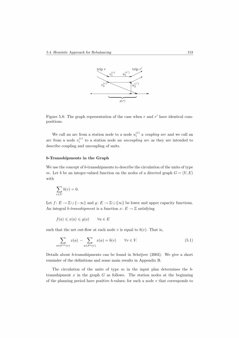
5.4. Heuristic Approach for Rebalancing 153
trip r trip r′
v(r)1
v(r)2
u(r′)1
u(r′)2
︸ ︷︷ ︸%(r)
Figure 5.8: The graph representation of the case when r and r′ have identical com-positions.
We call an arc from a station node to a node u(r)i a coupling arc and we call an
arc from a node v(r)i to a station node an uncoupling arc as they are intended to
describe coupling and uncoupling of units.
b-Transshipments in the Graph
We use the concept of b-transshipments to describe the circulation of the units of type
m. Let b be an integer-valued function on the nodes of a directed graph G = (V,E)
with
∑
v∈V
b(v) = 0.
Let f : E → Z∪ {−∞} and g : E → Z∪ {∞} be lower and upper capacity functions.
An integral b-transshipment is a function x : E → Z satisfying
f(a) 6 x(a) 6 g(a) ∀a ∈ E
such that the net out-flow at each node v is equal to b(v). That is,
∑
a∈δout(v)
x(a) −∑
a∈δin(v)
x(a) = b(v) ∀v ∈ V. (5.1)
Details about b-transshipments can be found in Schrijver (2003). We give a short
reminder of the definitions and some main results in Appendix B.
The circulation of the units of type m in the input plan determines the b-
transshipment x in the graph G as follows. The station nodes at the beginning
of the planning period have positive b-values; for such a node v that corresponds to
154 Chapter 5. Operational Rolling Stock Planning
station i, let b(v) be the number of units that start at station i. Similarly, the station
nodes at the end of the planning period have negative b-values; for such a node v
that corresponds to station i, let b(v) be the negative of the number of units that end
up at station i. For all other nodes, let b(v) = 0. This defines the function b. The
b-transshipment must be non-negative, the upper capacities are defined as follows.
For trip r, let µr be the largest number such that increasing the train length by µr
units of type m does not exceed the maximal allowed train length on trip r (denoted
by µmaxr ). Then the upper capacity of a trip arc u
(r)i v
(r)i is the size of the ith group
of trip r in the input plan plus µr. All other arcs have infinite upper capacity.
The x-value on trip arc u(r)i v
(r)i is the size of the ith group of trip r in the input
plan. The input plan explicitly says how many units of type m are coupled or
uncoupled before or after each trip, these are x-values on the coupling and uncoupling
arcs. The x-values on the remaining arcs are uniquely determined by constraints
(5.1).
Example. Figure 5.9(a) shows a railway network of two trips be-
tween stations A and B as the usual time-space diagram; both sta-
tions have left-hand shunting side. The riding direction does not
change between the two trips.
The input plan assigns a composition mm′ for both trips, the types
m and m′ are represented by black and grey units. Then the graph
is given in Figure 5.9(b). The function b : V → Z is defined as
b(v) =
1 if v = sA,
−1 if v = tA,
0 otherwise.
Bold arcs indicate the b-transshipment that arises from the input
plan: Bold arcs have x-value 1, other arcs have x-value zero.
We have seen above that a rolling stock circulation defines a b-transshipment in
the graph G = (V,E). Conversely, consider any specification for the initial and final
inventories and translate it into a function b′ : V → Z. Then each b′-transshipment
x′ defines a rolling stock circulation. However, the obtained rolling stock circulation
may violate some constraints of the problem specification. To avoid this, the following
two additional side constraints have to be fulfilled:
• The train length on each trip r obeys the lower and upper bounds:
µminr − Lr 6
∑
i
x′(u
(r)i v
(r)i
)6 µmax
r − Lr ∀ trip r (5.2)
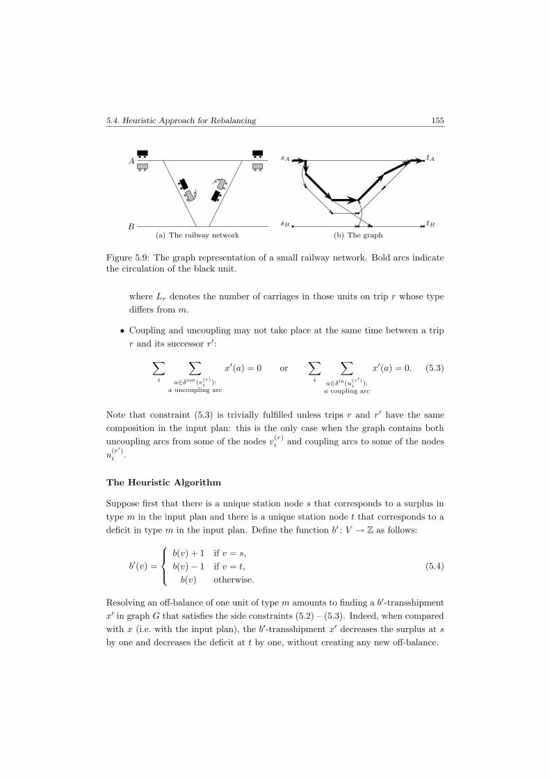
5.4. Heuristic Approach for Rebalancing 155
B
A
(a) The railway network
sA tA
sB tB
(b) The graph
Figure 5.9: The graph representation of a small railway network. Bold arcs indicatethe circulation of the black unit.
where Lr denotes the number of carriages in those units on trip r whose type
differs from m.
• Coupling and uncoupling may not take place at the same time between a trip
r and its successor r′:
∑
i
∑
a∈δout(v(r)i
):a uncoupling arc
x′(a) = 0 or∑
i
∑
a∈δin(u(r′)i
):a coupling arc
x′(a) = 0. (5.3)
Note that constraint (5.3) is trivially fulfilled unless trips r and r′ have the same
composition in the input plan: this is the only case when the graph contains both
uncoupling arcs from some of the nodes v(r)i and coupling arcs to some of the nodes
u(r′)i .
The Heuristic Algorithm
Suppose first that there is a unique station node s that corresponds to a surplus in
type m in the input plan and there is a unique station node t that corresponds to a
deficit in type m in the input plan. Define the function b′ : V → Z as follows:
b′(v) =
b(v) + 1 if v = s,
b(v) − 1 if v = t,
b(v) otherwise.
(5.4)
Resolving an off-balance of one unit of type m amounts to finding a b′-transshipment
x′ in graph G that satisfies the side constraints (5.2) – (5.3). Indeed, when compared
with x (i.e. with the input plan), the b′-transshipment x′ decreases the surplus at s
by one and decreases the deficit at t by one, without creating any new off-balance.

156 Chapter 5. Operational Rolling Stock Planning
Unfortunately, this problem is NP-hard: The proof of Theorem 5.5 can be re-
peated without any change. In the proof of the theorem, an off-balance of one unit
of type P has to be resolved, while the circulation of the other type Q is unaffected.
The heuristic algorithm looks for a b′-transshipment without taking the side con-
straints (5.2) – (5.3) into account, but afterwards it verifies whether (5.2) – (5.3) are
satisfied.
Heuristic rebalancing for an off-balance of one unit {
Create the graph G = (V,E).
Let s be the unique station node with a surplus.
Let t be the unique station node with a deficit.
Define b′ as in (5.4).
Look for a b′-transshipment x′ in G.
If x′ exists and satisfies (5.2) and (5.3) then
Accept the solution.
Else
Report that no solution was found.
}
It is known in network flow theory that, given the nodes s and t, such a b′-transship-
ment can be found efficiently as follows. Define the auxiliary graph G = (V, E). Start
from an empty graph on the node set V . For each arc uv ∈ E, add a forward arc
from u to v if x(uv) is smaller than the upper capacity of arc uv. For an arc uv ∈ E
with x(uv) > 0, add a backward arc from v to u. Let P be a directed s − t-path in
G. Then the function x′ : E → Z+ given by
x′(uv) =
x(uv) + 1 if the forward arc uv is used by path P ,
x(uv) − 1 if the backward arc vu is used by path P ,
x(uv) otherwise
(5.5)
is a b′-transshipment. Conversely, if there exists a b′-transshipment, then the aux-
iliary graph G contains a directed s − t-path. (For more details, see Appendix B.)
Therefore, the b′-transshipment x′ can be found in O(|E|) time by simply finding a
directed s − t-path in the auxiliary graph.
In the general case, there may be several candidates for the nodes s and t. This
can be handled in the same way as multiple-source multiple-sink single-commodity
flow problems: Add two new nodes s∗ and t∗ to the graph G, insert an arc s∗v for
each station node v that corresponds to a surplus of type m and insert an arc vt∗ for
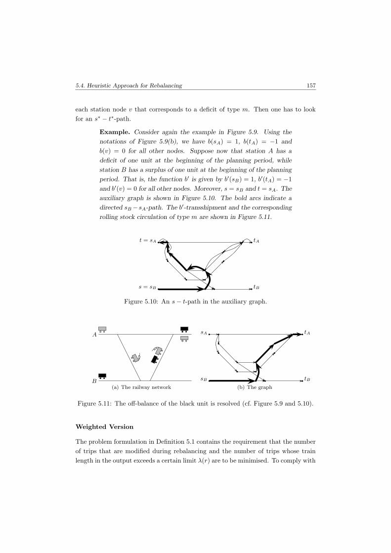
5.4. Heuristic Approach for Rebalancing 157
each station node v that corresponds to a deficit of type m. Then one has to look
for an s∗ − t∗-path.
Example. Consider again the example in Figure 5.9. Using the
notations of Figure 5.9(b), we have b(sA) = 1, b(tA) = −1 and
b(v) = 0 for all other nodes. Suppose now that station A has a
deficit of one unit at the beginning of the planning period, while
station B has a surplus of one unit at the beginning of the planning
period. That is, the function b′ is given by b′(sB) = 1, b′(tA) = −1
and b′(v) = 0 for all other nodes. Moreover, s = sB and t = sA. The
auxiliary graph is shown in Figure 5.10. The bold arcs indicate a
directed sB −sA-path. The b′-transshipment and the corresponding
rolling stock circulation of type m are shown in Figure 5.11.
t = sA tA
s = sB tB
Figure 5.10: An s − t-path in the auxiliary graph.
B
A
(a) The railway network
sA tA
sB tB
(b) The graph
Figure 5.11: The off-balance of the black unit is resolved (cf. Figure 5.9 and 5.10).
Weighted Version
The problem formulation in Definition 5.1 contains the requirement that the number
of trips that are modified during rebalancing and the number of trips whose train
length in the output exceeds a certain limit λ(r) are to be minimised. To comply with

158 Chapter 5. Operational Rolling Stock Planning
this specification, we assign cost values to the arcs of the auxiliary graph. The output
plan is obtained from the input plan by changing it along an s∗ − t∗-path. In the
weighted version of the heuristic approach, we choose a minimum cost s∗ − t∗-path.
Let r be a trip whose composition length in the input plan is not longer than λ(r)
but by coupling a unit of type m, the limit λ(r) is exceeded. As mentioned above,
this means that coupling an additional unit to trip r requires an extra conductor.
For such trips r, we assign a positive cost value to each forward arc u(r)i v
(r)i in
the auxiliary graph. Observe that these arcs express the possibility of making the
composition on trip r longer. The other cost component penalises the deviation from
the input plan: An additional positive cost is assigned to each forward arc u(r)i v
(r)i
and to each backward arc v(r)i u
(r)i . Using such an arc in the s∗ − t∗-path indicates
that the composition on trip r gets modified. Other arcs have zero cost.
Having defined these non-negative cost values, a minimum cost path can be found
very efficiently in O (|E| + |V | log |V |) time by Dijkstra’s algorithm using Fibonacci
heaps.
As it is often the case when modelling real-life problems, there are several choices
for the objective function. We point out here two possible adjustments for the case
when the algorithm for resolving an off-balance of one unit is used in an iterative
framework.
• The second cost component (that measures the deviation from the input plan)
compares the output plan with the last updated plan. In other words, if the
composition of a trip is adjusted in several iterations, the penalty is accounted
for several times. However, the problem specification in Definition 5.1 instructs
to minimise the deviation from the intermediate plan, i.e. from the plan at the
beginning of the rebalancing phase. An alternative cost structure may penalise
the modification of only those trips whose composition has not been adjusted
in the previous iterations.
• Suppose that a composition of trip r is increased in an iteration by a unit of
type m thereby requiring an extra conductor for trip r. In a later iteration, it
may be possible to resolve an additional off-balance of type m by decreasing
the composition of r. That is, after this latter iteration, no extra conductor
is needed again for trip r. So, it is actually advantageous to make use of a
backward arc v(r)i u
(r)i . This can be expressed by assigning a negative cost to
such backward trip arcs.
In our implementations, we do not take these two considerations into account.
The reason for this is that the main emphasis of this research is on deciding whether

5.4. Heuristic Approach for Rebalancing 159
the heuristic approach can handle the rebalancing problem at all. To that end, we
focus on the most important objective in rebalancing: to resolve as many off-balances
as possible. We leave fine-tuning the heuristic algorithm to minimise the other two
objective criteria for future research.
Off-balance of One unit Heuristically: Summary
We summarise the method for resolving an off-balance of one unit. The method tries
to resolve an off-balance of one unit subject to the constraint that the circulation of
all other rolling stock types remains unchanged.
First, create the graph G = (V,E) and compute the b-transshipment x from the
input plan as described above. Construct the auxiliary graph G, add the nodes s∗
and t∗ and insert the arcs to and from the station nodes with a surplus and a deficit,
respectively. Find a minimum cost directed s∗ − t∗-path P in G and construct the
b′-transshipment x′ according to (5.5).
We call a b′-transshipment good if it fulfils the side constraints (5.2) – (5.3),
otherwise we call it wrong. The heuristic algorithm returns x′ if it is a good b′-
transshipment, otherwise it rejects x′ reporting that it cannot resolve any off-balance
of type m.
If the algorithm returns a solution, then the output is a rolling stock circulation
that can be implemented in practise and that has one less off-balance than the input
plan. However, if the algorithm does not return a solution, it may have two reasons:
Either there does not exist any good b′-transshipment (in which case the outcome
of the algorithm is correct), or there exist good b′-transshipments but the algorithm
found a wrong one (in which case the outcome of the algorithm is incorrect). In
our computational tests, each b′-transshipment found by the heuristic algorithm was
good.
5.4.2 Arbitrary Off-balances Heuristically
For an instance of the rebalancing problem with arbitrary off-balances, we propose
a method that is similar to the heuristic algorithm in Section 4.5.8 for solving the
maintenance routing problem. We proceed iteratively, in each iteration resolving an
off-balance of a single unit and updating the intermediate plan accordingly. The
algorithm stops if it cannot resolve any more off-balances.

160 Chapter 5. Operational Rolling Stock Planning
The basic structure of the algorithm is as follows:
Heuristic rebalancing algorithm {
While there are off-balances {
M ′ := the set of types with off-balances.
Resolve an off-balance of one unit for an m ∈ M ′.
Stop if no off-balance could be resolved for any m ∈ M ′.
}
}
The number of iterations is at most the total number of off-balances. In each
iteration, each type m ∈ M ′ is tested at most once whether off-balances can be
resolved. For such a check for a fixed type, the running time is dominated by the
running time of Dijkstra’s algorithm O(|E|+|V | log |V |), since every other step – such
as building the graph, checking the side constraints and updating the rolling stock
circulation – is accomplished in O(|E|) time. The number of nodes and the number
of edges in the graph G are O(`T ) where T is the number of trips and ` is the largest
possible number of units in a composition. Therefore, the overall running time of
the heuristic rebalancing algorithm is O(kM`T log(`T )) where M is the number of
rolling stock types and k is the total number of off-balances. Note that different
instances of NSR share the same (small) numbers ` and M . That is, the running
time is essentially proportional to kT log T .
Whenever the algorithm terminates, its output is a rolling stock circulation that
satisfies all requirements. The question is, however, the quality of the solutions:
How many of the off-balances can be resolved in such a greedy way. In addition, one
may ask how many trips are modified in the rebalancing phase and how many trips
require an extra conductor. To answer these questions, we carried out computational
experiments. We report our results in the next section.
5.5 Computational Results
In this section we report our computational results on the rebalancing problem. As
described above, the rebalancing problem arises in the second phase of operational
rolling stock planning. The test instances used are not real-life problems of NSR. In-
stead, we take the tactical rolling stock circulation of the rolling stock type “Sprinter”
on two consecutive days and assume that this is the intermediate plan. To obtain
multiple types, we divide the available rolling stock into two types.

5.5. Computational Results 161
The test instances are generated from this intermediate plan as follows. We
assume that the final inventories of the intermediate plan have no off-balance and
we choose the off-balances of the initial inventories randomly. That is, we randomly
select the stations to have a surplus or a deficit in the initial inventory; the amount
of the surpluses and deficits is also chosen randomly. Of course, we take care that for
each rolling stock type the sum of the surpluses is equal to the sum of the deficits.
We solve each test instance in two different ways. In one approach, we formulate
it as an instance of the Composition Model and solve this model by the commercial
MIP software CPLEX 9.0 (using the modelling software ILOG OPL Studio 3.7).
We compare this with the other approach when we apply the heuristic rebalancing
algorithm implemented in the programming language Perl. All computations have
been carried out on a PC with a Pentium IV 3.0 GHz processor and 512 Mb internal
memory under the operating system Windows 98.
5.5.1 Dimensions of the Problem
The timetable in the test instances contains 803 trips between 12 stations. There are
47 units available, divided into two types of 21 and 26 units. The instances concern
an off-balance of 8 units: an off-balance of 4 units for both types. That is, the sum
of the surpluses is 4 for both types; also, the sum of the deficits is also 4 for both
types.
The Composition Model leads to a mixed integer program with 54,722 variables
(among them 17,636 integer variables) and 26,594 constraints. The reduced mixed
integer program has 53,753 variables, 25,888 constraints and 423,537 non-zeros in the
coefficient matrix. The heuristic method requires finding b-transshipments in a graph
with 4,200–4,400 nodes and 5,500–5,800 arcs. The essential part of the algorithm is
to find a minimum cost path in the auxiliary graph with the same number of nodes
and with about 7,300 arcs.
5.5.2 Objective Function
The objective function is a linear combination of the following three terms:
• 1000 times the amount of unresolved off-balances, summed for the two types,
• twice the number of trips that require an additional conductor,
• the number of trips whose composition is modified.

162 Chapter 5. Operational Rolling Stock Planning
zHeur0 Total number
0 1 2 3 4 of instanceszCM0 = 0 1,946 800 65 2 0 2,813
zCM0 = 1 1,322 269 9 0 1,600
zCM0 = 2 440 52 0 492
zCM0 = 3 87 6 93
zCM0 = 4 2 2Total 1,946 2,122 774 150 8 5,000
Table 5.1: Number of instances with given zCM0 and zHeur
0 .
Lacking information about the relative importance of the objective criteria, the co-
efficients 1000, 2 and 1 are chosen somewhat arbitrarily. In any case, the amount of
unresolved off-balances dominates the objective function.
The objective value of the Composition Model and of the heuristic rebalancing
method are denoted by zCM and zHeur, the amount of unresolved off-balances are
denoted by zCM0 and zHeur
0 .
5.5.3 Numerical Results
The first question is how many off-balances can be resolved by the heuristic method.
To answer it, we group the test instances according to the number of unresolved
off-balances, this gives Table 5.1. Table 5.2 shows the distribution of the value zHeur0
for each fixed value zCM0 . It turns out that in the vast majority of the instances, the
heuristic method leaves at most one more unresolved off-balance than the Composi-
tion Model does. Actually, in about 75% of the instances (in 3,797 cases of 5,000) the
two methods resolve the same amount of off-balances. It indicates that for most test
instances, the smaller solution space of the heuristic approach still includes solutions
with an (almost) minimal number of off-balances and that the very simple heuristic
algorithm is able to find these solutions.
We compare the objective values of the instances for which the Composition
Model and the heuristic approach resolved the same amount of off-balance. Table 5.3
contains the average and maximum values of zCM as well as the average and maximum
difference of zHeur − zCM. The averages and the maxima are computed separately
for each given value zCM0 . Note that the line for zCM
0 = zHeur0 = 4 concerns only two
instances.
For the number of trips that require an extra conductor and for the number
of trips that are modified, solutions of the heuristic method have 50–100% higher
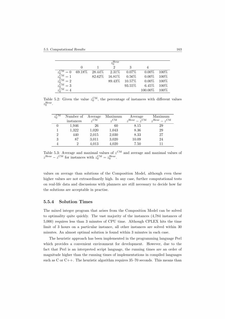
5.5. Computational Results 163
zHeur0
0 1 2 3 4zCM0 = 0 69.18% 28.44% 2.31% 0.07% 0.00% 100%
zCM0 = 1 82.62% 16.81% 0.56% 0.00% 100%
zCM0 = 2 89.43% 10.57% 0.00% 100%
zCM0 = 3 93.55% 6.45% 100%
zCM0 = 4 100.00% 100%
Table 5.2: Given the value zCM0 , the percentage of instances with different values
zHeur0 .
zCM0 Number of Average Maximum Average Maximum
instances zCM zCM zHeur − zCM zHeur − zCM
0 1,946 26 60 8.15 291 1,322 1,020 1,043 8.36 292 440 2,015 2,030 8.33 273 87 3,011 3,020 10.09 244 2 4,013 4,020 7.50 11
Table 5.3: Average and maximal values of zCM and average and maximal values ofzHeur − zCM for instances with zCM
0 = zHeur0 .
values on average than solutions of the Composition Model, although even these
higher values are not extraordinarily high. In any case, further computational tests
on real-life data and discussions with planners are still necessary to decide how far
the solutions are acceptable in practise.
5.5.4 Solution Times
The mixed integer program that arises from the Composition Model can be solved
to optimality quite quickly. The vast majority of the instances (4,784 instances of
5,000) requires less than 3 minutes of CPU time. Although CPLEX hits the time
limit of 3 hours on a particular instance, all other instances are solved within 30
minutes. An almost optimal solution is found within 3 minutes in each case.
The heuristic approach has been implemented in the programming language Perl
which provides a convenient environment for development. However, due to the
fact that Perl is an interpreted script language, the running times are an order of
magnitude higher than the running times of implementations in compiled languages
such as C or C++. The heuristic algorithm requires 35–70 seconds. This means than

164 Chapter 5. Operational Rolling Stock Planning
the same algorithm implemented in C++ would very likely achieve running times of
a couple of seconds.
5.6 Conclusions and Future Work
In this chapter we discussed the operational rolling stock circulation problem. The
methods described in Chapter 3 can be adapted to it. In particular, solving the
Composition Model by commercial MIP software gives promising results in compu-
tational tests, although further investigation is needed concerning the performance
of the method on operational rolling stock planning instances that are substantially
larger than the test problems.
As an alternative approach, we considered a model-based version of the two-
phase method that is applied currently at NSR. Focusing on the second phase only,
we formulated the rebalancing problem, discussed its computational complexity and
proposed a heuristic solution method. The Composition Model can be adapted to the
rebalancing problem, too. This allows one to evaluate the performance of the heuristic
approach by comparing its output with the optimal solutions of the Composition
Model.
Computational experiments revealed that, despite its simplicity, the heuristic
approach very often resolves the largest possible number of off-balances or just one
less. Thus we can conclude that it is in fact plausible to use a heuristic algorithm of
such a kind as a planning tool. The advantage of such a method is that its running
time remains attractively low, even for problem sizes when the memory consumption
and solution time of the Composition Model may become a bottleneck.
Our research on operational rolling stock planning problems is not completed
with the results of this chapter. Concerning the two-phase approach, automating the
process of creating the intermediate plan as well as extending the two-phase method
for instances with splitting and combining is a subject of further research.
Moreover, the usefulness of any solution method is not only measured by the
value of the objective criteria, but also by its flexibility and its actual contribution in
speeding up the operational rolling stock planning process. The evaluation of both
the Composition Model and the heuristic approach on real-life instances also belongs
to our future plans.

Chapter 6
Conclusions and Future Work
In this thesis we considered various rolling stock planning problems that arise at the
major Dutch passenger railway operator NSR. In Chapter 2, we gave an overview of
the planning process. This describes the context for the particular planning problems
studied in this thesis. The subsequent chapters are devoted to tactical, short-term
and operational rolling stock planning problems.
6.1 Main Results
Tactical Rolling Stock Circulations
In Chapter 3 we studied the tactical rolling stock circulation problem where the
available rolling stock is to be assigned to the trains such that various technical and
market requirements are fulfilled. The objective is to find a good balance of efficiency,
service quality and robustness.
We formulated the Composition Model which is a mixed integer programming
model. Extensive computational tests show that by using commercial MIP software
for solving it, the model provides good solutions within a couple of hours even for
the most difficult instances of NSR; usual instances are solved to optimality within
minutes. Planners at NSR agree that the solutions of this model are in any respect
better than the manually created rolling stock circulations. From 2004 on, the Com-
position Model is used at NSR to specify the basic shape of the rolling stock plan.
This allowed to decrease the number of carriage-kilometres significantly and thereby
to reduce the annual rolling stock costs of NSR by a couple of millions of euros.
As an additional benefit, tactical rolling stock planning at NSR became faster and
165

166 Chapter 6. Conclusions and Future Work
smoother. It is possible now to work out and compare rolling stock circulations with
different characteristics when looking for the best balance of the objective criteria.
We also formulated the Job Model which is an alternative approach for tactical
rolling stock circulations. This model has the drawback that it cannot handle splitting
and combining of trains, a feature that occurs in some real-life instances. Also,
computational tests revealed that the Composition Model clearly outperforms the
Job Model.
We can conclude that operations research techniques can be used to model tac-
tical rolling stock circulations. In particular, the Composition Model has proved its
usefulness in practise.
Maintenance Routing
In Chapter 4 we described the maintenance routing problem of NSR. It arises in
short-term planning, a couple of days before the rolling stock plans are to be carried
out. Units that travelled a high number of kilometres since their last preventive
maintenance check must be routed to the maintenance facilities by modifying the
rolling stock plan of the forthcoming couple of days.
We formulated two multi-commodity flow type models for maintenance routing:
the Interchange Model and the Transition Model. The Interchange Model needs a
vast amount of input data about the shunting process which may not be available in
practise; the Transition Model is a much simpler formulation. When one chooses ap-
propriate objective functions, the Transition Model is a relaxation of the Interchange
Model.
We proved the following complexity results. The feasibility problem of the Inter-
change Model is NP-complete if the number of urgent units is part of the input. With
mild assumptions about the input, the optimisation version of the Interchange Model
can be solved in polynomial time in the case of a single urgent unit. The feasibility
of the Transition Model with a single urgent unit can be checked in polynomial time
in graphs that arise in railway applications. However, the optimisation version of the
Transition Model in such graphs is NP-hard.
We proposed a heuristic solution approach for the Interchange Model. In our
computational experiments it turned out that the heuristic approach is able to solve
all test instances. Easy-to-compute lower bounds verify that the heuristic solutions
have a small absolute optimality gap. The integer programming formulation of the
Interchange Model and the Transition Model can also be solved by commercial MIP
solvers in reasonable time. When solving both models on the same instances, the
optimal solution values of the two models did not differ much. This indicates that

6.1. Main Results 167
the simpler Transition Model underestimates the solution costs of the Interchange
Model only slightly.
We discussed a number of our solutions with maintenance routing planners; they
found them satisfactory. Thus we can conclude that it is plausible to use any of
the Interchange Model and the Transition Model in a decision support system for
maintenance routing. Investigating the actual usefulness of the models in practise is
a subject of further research.
Operational Planning: Rebalancing
In Chapter 5 we discussed operational rolling stock circulations. Operational plan-
ning takes the tactical rolling stock schedules as input and adjusts them for the
forthcoming couple of weeks. The problem formulation is very close to that in tacti-
cal planning, but the objective differs. The main goal is that the operational plans
(including the shunting plans) are accomplished as quickly as possible. Currently, a
two-phase approach is applied at NSR. The first phase sets up an intermediate plan
which may violate inventory specifications. In the second phase, these off-balances
are resolved.
In this thesis we only focused on the second phase, called rebalancing. We proved
that the feasibility of the rebalancing problem is NP-complete even for an off-balance
of only one unit. Then we proposed an iterative heuristic rebalancing algorithm.
The Composition Model can easily be adapted for the rebalancing problem. So
we considered rebalancing instances of NSR, formulated them as instances of the
Composition Model and solved them using commercial MIP software. Also, we ran
the heuristic algorithm on these test instances and compared the results of the two
methods.
It turned out that on these instances the Composition Model can be solved to
optimality within a couple of minutes. Despite its greedy character, for most test
instances the heuristic approach is able to resolve the same number of off-balances
as the Composition Model or just one less. We can conclude that it is plausible to
apply the heuristic algorithm to the rebalancing problem.
Real-life operational planning instances can be significantly larger and more com-
plex than the test instances we considered. The heuristic approach has the advantage
that its running time is moderate, even on huge instances. Further research is needed,
however, to examine the behaviour of both methods on large instances: the solution
time of the Composition Model and the solution quality of the heuristic approach.
168 Chapter 6. Conclusions and Future Work
6.2 Future Work
The results of this thesis indicate that the models and solution methods have the
potential to become the core of useful planning tools. However, many questions
remain open, further investigations are necessary to answer them.
We have seen that the Composition Model is able to handle each tactical rolling
stock circulation instance of NSR. However, these instances are obtained by decom-
posing the railway network into line groups and by considering one day only. A
natural question is whether instances with several line groups on several consecutive
days are still tractable and how much one can gain by planning the rolling stock in
that way.
The practical value of the maintenance routing models has still to be verified. So
far, we only had feedback from maintenance routing planners. Future research has
to involve local planners into the evaluation of the models in order to decide whether
the output of the models can be carried out in practise. In addition, systematic com-
parison of the output of our models with solutions of maintenance routing planners
is needed to refine the models and to get an objective function that reflects reality
as well as possible.
Our research on operational rolling stock planning has just started. In the context
of the two-phase method of NSR, the first phase still needs to be addressed. Then the
fully automated two-phase method is to be tested on real-life instances. Investigating
the performance of the Composition Model on real-life operational planning problems
also belongs to our future plans.
Besides the three rolling stock planning problems that we studied in this thesis,
many other ones still wait for computer-aided tools. For example, there are barely
tools for short-term planning, in particular for disruption management; this is quite
in contrast with successful tactical planning applications and even with on-going
research on operational planning. Further research has to explore solution methods
for such railway problems.
So far we discussed results and directions for future work mainly from the oper-
ations research’s point of view. We evaluated the solution quality and solving time
of the models on real-life instances although we noted that the contribution of most
of our models to railway planning still needs to be investigated. But even when the
solutions of the models turn out to be the solutions of the railway problems, this
is just the first step to build decision support tools. The solution methods have
to be integrated into the planning process, this raises questions that reach beyond
operations research.
6.2. Future Work 169
Unified databases have to be built up so that the input of the models can be
gathered automatically. This is especially important in short-term planning where
the input has to reflect the very latest state of the railway system. The output of the
models has to be evaluated by human planners. User-friendly interfaces are required
to be able to interpret the output easily. A well-designed user interface can help
operations research methods to gain acceptance in everyday railway planning.
Once these tasks are accomplished, the railway operators can take full benefit
of the planning tools built upon operations research models. The case of tactical
rolling stock circulations proves that there is a lot to gain by using such tools, not
only financially but also in the flexibility and the speed of the planning process. We
look forward to see a similarly successful application of our other models in railway
planning in the near future.

Appendix A
Glossary
In this appendix we provide our understanding of railway terminology. The expla-
nations below are intended to be short reminders. The terms are described more
precisely in the previous sections. The index helps finding these definitions.
Unit: Two to six railway carriages attached to each other, supplied with own en-
gines and having driver’s cabin at both ends. Units cannot be split up during
everyday operations.
Type: A group of units that have identical technical parameters and seat capacities.
Physical units of the same type are only distinguished by their mileage.
Composition: Units attached to each other in a given order. In short-term plan-
ning, the members of a composition are the physical units. In tactical and
operational planning, compositions are specified only by their type patterns.
Shunting: Movements of units inside the stations. Shunting also includes putting
temporarily not used units to storage tracks and adjusting train lengths between
an arrival and the subsequent departure by coupling or uncoupling some units.
Train: A movement of units that makes use of tracks between different stations. A
train is characterised by the train number, the departure and arrival locations,
the route through the railway infrastructure, the departure and arrival times
and usually with the departure and arrival platforms.
Timetable: The description of all trains.
Timetable service: A train that may carry passengers.
171

172 Appendix A. Glossary
Empty train: A train that does not carry passengers, used for repositioning units
from one location to another.
Successor train of an arriving train: planned to be carried out by the units that
served in the arriving train. Yet, minor composition changes may be possible.
Usually, trains have zero or one successor. In case of splitting, a train has two
successors. Note that the notion of successors also applies to trips and tasks.
Predecessor train: the opposite of successors. Note that the notion of predecessors
also applies to trips and tasks.
Turn-around: the pair of events formed by the arrival of a train and the departure
of its successor train together with the intermediate occupation of a platform
track.
Coupling: Attaching units from the inventory to a departing train.
Uncoupling: Detaching units from an arriving train and adding them to the inven-
tory.
Composition change: Coupling or uncoupling units during a turn-around.
Inventory: The number of units per type that are stored at a station at a given
moment. The inventory contains only units that are ready to be used in any
departing train. That is, we do not count those units that depart from a station
soon after the arrival.
Splitting of trains occurs when an arriving train has two successors.
Combining of trains occurs when a departing train has two predecessors.
Train line: A series of timetable services that call at given stations. Train lines are
operated with a given frequency, e.g. twice an hour.
Line group: A system of interconnected train lines. Most line groups have (almost)
closed rolling stock circulations. That is, the daily workload of most units
consists of train movements that belong to the same line group.
Trip: A sequence of train movements that has to be carried out without composition
changes. Trips are the basic objects in tactical and operational planning. A
timetable service that admits composition changes underway consists of several
trips. The notion of successor and predecessor trains applies also to trips.

Appendix A. Glossary 173
Tasks: The smallest indivisible piece of work to be carried out by a single unit. A
task is characterised by a trip and a position in the composition that is assigned
to the trip. The notion of successor and predecessor trains applies also to tasks.
Duty: The workload of an employee or of a unit for a certain period, usually a day.
The duty of a rolling stock unit is a sequence of tasks.
Rolling stock circulation: The collection of the rolling stock duties for a certain
period, e.g. for a day. It assigns units to the trains and describes the order
of the units in the compositions. Rolling stock circulations of consecutive days
must fit to each other: at each station, the inventory at the end of a day must
be equal to the inventory at the beginning of the next day.


Appendix B
b-Transshipments
In this appendix we define the notion of b-transshipments and mention some impor-
tant properties. The definitions and theorems below are well-known in the theory
of network flows. For more details, we refer to Schrijver (2003). In this thesis we
only consider integer-valued b-transshipments, therefore we restrict ourselves to the
integer-valued cases.
B.1 Definition of a b-Transshipment
Let G = (V,E) be a directed graph, let f : E → Z∪{−∞} and let g : E → Z∪{∞} be
lower and upper capacity functions with f(e) 6 g(e) for every e ∈ E. Let b : V → Z
with∑
v∈V b(v) = 0.
Definition B.1. The function x : E → Z is a b-transshipment if the following two
requirements hold:
f(a) 6 x(a) 6 g(a) ∀a ∈ E, (B.1)∑
a∈δoutv
x(a) −∑
a∈δinv
x(a) = b(v) ∀v ∈ V. (B.2)
The latter constraint expresses that, using the terminology of network flows, the
net out-flow of each node v is equal to b(v).
For example, a network flow with one unit of flow from the source s to the sink
t and with arc capacities g : E → Z ∪ {∞} is a b-transshipment by setting f(e) = 0
175

176 Appendix B. b-Transshipments
for each arc e and by defining
b(v) =
1 if v = s,
−1 if v = t,
0 otherwise.
(B.3)
In general, a b-transshipment can be considered as a multiple-source multiple-sink
network flow problem: The nodes with b(v) > 0 are the sources with out-flow b(v),
while the nodes with b(v) < 0 are the sinks with in-flow −b(v). This construction
allows to carry over many results of network flows to b-transshipments.
B.2 Auxiliary Graph
The auxiliary graph G = (V, E) associated with a b-transshipment x is defined as
follows. The graph G has the same node set as the graph G. For u, v ∈ V , graph G
has a forward arc uv if uv ∈ E and x(uv) < g(uv). That is, if the value of x can be
increased on arc uv without violating the upper capacities. For u, v ∈ V , graph G
has a backward arc vu if uv ∈ E and x(uv) > f(uv). That is, if the value of x can
be decreased on arc uv without violating the lower capacities.
For any subset F ⊆ E, we define the function χF : E → Z as follows. For each
arc uv ∈ E, let
χF (uv) =
1 if uv ∈ E and vu /∈ E,
−1 if vu ∈ E and uv /∈ E,
0 otherwise.
(B.4)
B.3 Results on b-Transshipments
In this thesis we use the following facts about b-transshipments. Let s, t ∈ V and
define b′ : V → Z as
b′(v) =
1 if v = s,
−1 if v = t,
0 otherwise.
(B.5)
Theorem B.2. Let x be an integral b-transshipment and let P be a directed s−t-path
in the auxiliary graph G. Then
x′ = x + χP (B.6)
B.3. Results on b-Transshipments 177
is a b′-transshipment.
Theorem B.3. Let x be an integral b-transshipment and let x′ be an integral b′-
transshipment. Then the auxiliary graph G contains a directed s − t-path P and
directed circuits Ci such that
x′ = x + χP +∑
i
χCi . (B.7)
Corollary B.4. Let x be an integral b-transshipment and suppose that there exists
a b′-transshipment. Then the auxiliary graph G contains a directed s − t-path.


Appendix C
Notations
This appendix gathers all symbols used as parameters and variables for the models
in this thesis.
C.1 Notations in Chapter 3
Parameters for Both Models
M the set of rolling stock types
nm number of available units of type m
cm number of carriages in a unit of type m
`m length of a unit of type m (in metres)
C the set of service classes
κm,c seat capacity of a unit of type m for service class c
S set of stations
i0s,m wished initial inventory of station s in type m
i∞s,m wished final inventory of station s in type m
Ws storage capacity of station s (in metres)
T the set of trips
sd (t) departure station of trip t
τd (t) departure time of trip t
sa (t) arrival station of trip t
τa (t) arrival time of trip t
dt length of trip t (in kilometres)
% (t) re-allocation time after trip t
179

180 Appendix C. Notations
µmint minimum number of carriages to be assigned to trip t
µmaxt maximum number of carriages to be assigned to trip t
δt,c passenger demand on trip t for service class c
σ (t) successor of trip t
T0 the set of trips without predecessors
T∞ the set of trips without predecessors
σ1 (t), σ2 (t) successors of trip t in case of splitting
Ts the set of trips the are split
Tc the set of trips the are combined
Specific Parameters for the Composition Model
|p| total number of units in composition p
ν(p)m number of units of type m in composition p
Pt the set of compositions that can be assigned to trip t
Bt the set of vectors ν(p) that can be assigned to trip t
Gt the set of allowed composition changes after trip t
Gs the set of allowed composition changes when trip t is split
Gc the set of allowed composition changes when trip t is combined
Specific Parameters for the Job Model
J the set of jobs
Rj the set of trips covered by job j
ϕj first trip covered by job j
ϕj last trip covered by job j
sd (j) departure station of job j
sd (j) time station of job j
τa (j) arrival station of job j
τa (j) arrival time of job j
dj length of job j (in kilometres)
µj upper bound on the number of units that can be assigned to
job j
µj upper bound on the number of carriages that can be assigned
to job j
γd(t) coupling side of ϕj
γa(t) uncoupling side of λj

C.1. Notations in Chapter 3 181
Variables for the Composition Model
Xt,p whether composition p is assigned to trip t
Zt,p,p′ whether composition change p → p′ occurs after trip t
Nt,m number of units of type m assigned to trip t
Ct,m number of units of type m coupled to trip t
Ut,m number of units of type m uncoupled from trip t
I0s,m initial inventory of station s in type m
I∞s,m final inventory of station s in type m
It,m inventory of station sd (t) in type m right after trip t departs
Yt,b whether a combination b ∈ Bt is assigned to trip t
CKM carriage-kilometres
SKM seat-shortage kilometres
CCH the number of composition changes
Zst,p,p1,p2
whether trip t with composition p is split into compositions
p1 and p2
Zct,p,p1,p2
whether trip t with composition p is combined from composi-
tions p1 and p2
ZUtt,p,p1,...,p6
whether splitting-combining scenario (p, p1, p2, p3, p4, p5, p6)
is selected after trip t
CGvc whether any unit is coupled in The Hague in the selected
splitting-combining scenario
CRtd whether any unit is coupled in Rotterdam in the selected
splitting-combining scenario
UGvc whether any unit is uncoupled in The Hague in the selected
splitting-combining scenario
URtd whether any unit is uncoupled in Rotterdam in the selected
splitting-combining scenario
Variables for the Composition Model
Xj whether job j is selected
Nj,m number of units of type m assigned to job j
Ht whether a composition change takes place right before trip t
I0s,m initial inventory of station s in type m
I∞s,m final inventory of station s in type m
Ij,m inventory of station sd (j) in type m right after job j departs
St,c seat-shortage of service class c on trip t

182 Appendix C. Notations
C.2 Notations in Chapter 4
Parameters for Both Models
sd (t) departure station of task t
sd (t) time station of task t
τa (t) arrival station of task t
τa (t) arrival time of task t
σ (t) successor of task t
% buffer time
U the set of urgent nodes
M the set of maintenance nodes
Mu the set of maintenance nodes that can be assigned to urgent
node u
Parameters for the Interchange Model
D number of available units
H length of the planning horizon (in minutes)
I the set of interchanges
V0 the set of first nodes
V∞ the set of last nodes
stat(v) station corresponding to node v of the graph representation
time(v) time corresponding to node v of the graph representation
tail(a) the tail node of a directed arc a
head(a) the head node of a directed arc a
weight(a) weight of an arc
Specific Parameters for the Transition Model
V0 the set of source nodes of the acyclic graph
V∞ the set of source nodes of the acyclic graph
c weight of a transition
c weight of a transition derived from the Interchange Model

C.3. Notations in Chapter 5 183
Variables for the Interchange Model
yC whether interchange C is selected
z(a) network flow that indicates the paths of all units through the
entire planning horizon
xu(a) a network flow that indicates the path of urgent unit u to a
maintenance task
Variables for the Transition Model
z(a) network flow that indicates the paths of all units through the
entire planning horizon
xu(a) a network flow that indicates the path of urgent unit u to a
maintenance task
C.3 Notations in Chapter 5
sd (r) departure station of trip r
sd (r) time station of trip r
τa (r) arrival station of trip r
τa (r) arrival time of trip r
% (r) re-allocation time after trip r
µminr minimum number of carriages to be assigned to trip r
µmaxr maximum number of carriages to be assigned to trip r
λ(r) an extra conductor is needed for trip r if it is assigned more
than λ(r) carriages
µr maximum number of units of type m that can be added to
trip r without exceeding the maximal train length µmaxr
Lr the number of carriages in those units on trip r whose type
differs from the given type m


Bibliography
Abbink, E.J.W, Fischetti, M., Kroon, L.G., Timmer, G., Vromans,
M.J.C.M. (2005). Reinventing Crew Scheduling at Netherlands Railways. In-
terfaces, 35(5):393–401.
Abbink, E.J.W, Van der Berg, B.W.V., Kroon, L.G., Salomon, M. (2004).
Allocation of Railway Rolling Stock for Passenger Trains. Transportation Science,
38(1):33–42.
Alfieri, A., Groot, R., Kroon, L.G., Schrijver, A. (2002). Efficient Circula-
tion of Railway Rolling Stock . ERIM Research Report ERS-2002-110-LIS, Erasmus
University Rotterdam, The Netherlands. Submitted to Transportation Science.
Anderegg, L., Eidenbenz, S., Gantenbein, M., Stamm, Ch., Taylor, D.S.,
Weber, B., Widmayer, P. (2003). Train Routing Algorithms: Concepts, Design
Choices, and Practical Considerations. In Proceedings of ALENEX’03 .
http://www.siam.org/meetings/alenex03/Abstracts/LAnderegg3.pdf.
Anthony, R.N. (1965). Planning and Control Systems: A Framework for Analysis.
Harvard University, Boston.
Assad, A.A. (1980). Models for Rail Transportation. Transportation Research A,
14:205–220.
Barnhart, C., Boland, N.L., Clarke, L.W., Johnson, E.L., Nemhauser,
G.L., Shenoi, R.G. (1998a). Flight String Models for Aircraft Fleeting and Rout-
ing . Transportation Science, 32(3):208–220.
Barnhart, C., Johnson, E.L., Nemhauser, G.L., Savelsbergh, M.W.P.,
Vance, P.H. (1998b). Branch-and-Price: Column Generation for Solving Huge
Integer Programs. Operations Research, 46:316–329.
185

186 BIBLIOGRAPHY
Ben-Khedher, N., Kintanar, J., Queille, C., Stripling, W. (1998). Schedule
Optimization at SNCF: From Conception to Day of Departure. Interfaces, 28:6–23.
Bertossi, A.A., Carraresi, P., Gallo, G. (1987). On Some Matching Problems
Arising in Vehicle Scheduling Models. Networks, 17:271–281.
Blasum, U., Bussieck, M.R., Hochstattler, W., Moll, C., Scheel, H.H.,
Winter, T. (2000). Scheduling Trams in the Morning . Mathematical Methods
of Operations Research, 49:137–148.
Brucker, P., Hurink, J., Rolfes, T. (1998). Routing of Railway Carriages: A
Case Study . Osnabrucker Schriften zur Mathematik, Reihe P, Heft 205.
Bussieck, M.R. (1998). Optimal Line Plans in Public Rail Transport . Ph.D. thesis,
Braunschweig University of Technology, Germany.
Caprara, A., Fischetti, M., Toth, P. (1999). A Heuristic Algorithm for the
Set Covering Problem. Operations Research, 47:730–743.
Caprara, A., Fischetti, M., Toth, P., Vigo, D. (1998). Modeling and Solving
the Crew Rostering Problem. Operations Research, 46:820–830.
Carraresi, P., Gallo, G. (1984). Network Models for Vehicle and Crew Schedul-
ing . European Journal of Operational Research, 16:139–151.
Clarke, L., Johnson, E., Nemhauser, G., Zhu, Z. (1997). The Aircraft Rotation
Problem. Annals of Operations Research, 69:33–46.
Cook, S.A. (1971). The Complexity of Theorem-proving Procedures. In Conference
Record of Third Annual ACM Symposium on Theory of Computing , pages 151–158.
The Association for Computing Machinery, New York.
Cordeau, J.F., Desaulniers, G., Lingaya, N., Soumis, F., Desrosiers, J.
(2001a). Simultaneous Locomotive and Car Assignment at VIA Rail Canada.
Transportation Research B, 35:767–787.
Cordeau, J.F., Soumis, F., Desrosiers, J. (2000). A Benders Decomposition Ap-
proach for the Locomotive and Car Assignment Problem. Transportation Science,
34:133–149.
——– (2001b). Simultaneous Assignment of Locomotives and Cars to Passenger
Trains. Operations Research, 49:531–548.
BIBLIOGRAPHY 187
Cordeau, J.F., Toth, P., Vigo, D. (1998). A Survey of Optimization Models for
Train Routing and Scheduling . Transportation Science, 32:380–404.
Desrosiers, J., Dumas, Y., Solomon, M.M., Soumis, F. (1995). Time Con-
strained Routing and Scheduling . In Ball, M.O. (editor), Handbooks in Oper-
ations Research and Management Science, volume 8: Network Routing, pages
35–139. Elsevier.
Feo, T.A., Bard, J.F. (1989). Flight Scheduling and Maintenance Base Planning .
Management Science, 35(12):1514–1532.
Fioole, P.J., Kroon, L.G., Maroti, G., Schrijver, A. (2004). A Rolling Stock
Circulation Model for Combining and Splitting of Passenger Trains. CWI Research
Report PNA–E0420, Center for Mathematics and Computer Science, Amsterdam,
The Netherlands. To appear in European Journal of Operational Research.
Fores, S., Proll, L., Wren, A. (2001). Experiences with a Flexible Driver Sched-
uler . In Voß, S., Daduna, J.R. (editors), Computer-Aided Scheduling of Public
Transport , pages 137–152. Springer, Berlin, Germany.
Freling, R., Lentink, R.M., Kroon, L.G., Huisman, D. (2005). Shunting of
Passenger Train Units in a Railway Station. Transportation Science, 39(2):261–
272.
Gallo, G., di Miele, F. (2001). Dispatching Buses in Parking Depots. Trans-
portation Science, 35:379–393.
Goossens, J.H.M. (2004). Models and Algorithms for Railway Line Planning Prob-
lems. Ph.D. thesis, University of Maastricht, The Netherlands.
Gopalan, R., Talluri, K.T. (1998). The Aircraft Maintenance Routing Problem.
Operations Research, 46(2):260–271.
Groot, R. (1996). Minimum Circulation of Railway Stock . Master’s thesis, Uni-
versity of Amsterdam, The Netherlands.
Haghani, A., Shafahi, Y. (2002). Bus Maintenance Systems and Maintenance
Scheduling: Model Formulations and Solutions. Transportation Research Part A,
36:453–482.
Hooghiemstra, J.S. (1996). Design of Regular Interval Timetables for Strategic
and Tactical Railway Planning . In Allan, J., Brebbia, C.A., Hill, R.J.,
Sciutto, G. (editors), Computers in Railwais V , volume 1, pages 393–402. WIT
Press, Southampton, United Kingdom.

188 BIBLIOGRAPHY
Hooghiemstra, J.S., Kroon, L.G., Odijk, M.A., Salomon, M., Zwaneveld,
P.J. (1999). Decision Support Systems Support the Search for Win-win Solutions
in Railway Network Design. Interfaces, 29(2):15–32.
Huisman, D., Kroon, L.G., Lentink, R.M., Vromans, M.J.C.M. (2005). Op-
erations Research in Passenger Railway Transportation. Statistica Neerlandica,
59(4):467–497.
Karp, R.M. (1972). Reducibility among Combinatorial Problems. In Miller, R.E.,
Thatcher, J.W. (editors), Complexity of Computer Computations, pages 85–103.
Plenum Press, New York.
Karzanov, A.V. (1970). An Efficient Algorithm for Finding All the Bicomponents
of a Graph. In Third Winter School on Mathematical Programming and Related
Topics, pages 343–347. Vypusk II, MISI, Moscow. In Russian.
Kohl, N. (2003). Solving the World’s Largest Crew the Scheduling Problem. ORbit
Extra, pages 8–12. Danish Operations Research Society.
Kohl, N., Karish, S.E. (2004). Airline Crew Rostering: Problem Types, Modeling
and Optimization. Annals of Operations Research, 127:223–257.
Kroon, L.G., Fischetti, M. (2001). Crew Scheduling for Netherlands Railways
“Destination: Customer”. In Voß, S., Daduna, J.R. (editors), Computer-Aided
Scheduling of Public Transport , pages 181–201. Springer, Berlin, Germany.
Lentink, R.M. (2006). Algorithmic Decision Support for Shunt Planning . Ph.D.
thesis, Erasmus University Rotterdam, The Netherlands.
Lentink, R.M., Fioole, P.J., Kroon, L.G., Van ’t Woudt, C. (2003). Op-
erations Research in Passenger Railway Transportation. ERIM Research Report
ERS-2003-094-LIS, Erasmus University Rotterdam, The Netherlands.
Lingaya, N., Cordeau, J.F., Desaulniers, G., Desrosiers, J., Soumis, F.
(2002). Operational Car Assignment at VIA Rail Canada. Transportation Re-
search B, 36:755–778.
Maroti, G., Kroon, L.G. (2004). Maintenance Routing for Train Units: the
Scenario Model . CWI Research Report PNA–E0414, Center for Mathematics and
Computer Science, Amsterdam, The Netherlands. Revised version to appear in
Computers and Operations Research.
——– (2005). Maintenance Routing for Train Units: the Transition Model . Trans-
portation Science, 39(4):518–525.

BIBLIOGRAPHY 189
NS Intranet (2005). http://insite.ns.nl.
Peeters, L.W.P. (2003). Cyclic Railway Timetable Optimization. Ph.D. thesis,
Erasmus University Rotterdam, The Netherlands.
Peeters, M., Kroon, L.G. (2003). Circulation of Railway Rolling Stock: a Branch-
and-Price Approach. ERIM Research Report ERS-2003-055-LIS, Erasmus Uni-
versity Rotterdam, The Netherlands. To appear in Computers and Operations
Research.
Poort, J.P. (2002). Grenzen aan Benutting (Limits on Utilisation). NYFER,
Breukelen, The Netherlands. In Dutch.
Scholl, S. (2001). Anschlusssicherungen bei Verspatungen in OPNV (Securing
Connections in Case of Delays at OPNV). Master’s thesis, University of Kaiser-
slautern, Germany. In German.
——– (2005). Customer Oriented Line Planning . Ph.D. thesis, Kaiserslautern Uni-
versity of Technology, Germany.
Schrijver, A. (1993). Minimum Circulation of Railway Stock . CWI Quarterly,
6:205–217. Center for Mathematics and Computer Science, Amsterdam, The
Netherlands.
Schrijver, A. (2003). Combinatorial Optimization: Polyhedra and Efficiency .
Springer Verlag, Berlin, Heidelberg.
Schrijver, A., Steenbeek, A. (1994). Dienstregelingontwikkeling voor RailNed
(Timetable Construction for RailNed). Technical report, Center for Mathematics
and Computer Science, Amsterdam, The Netherlands. In Dutch.
Schulz, F., Wagner, D., Zaroliagis, C. (2002). Using Multi-Level Graphs for
Timetable Information in Railway Systems. In Proceedings 4th Workshop on Al-
gorithm Engineering and Experiments (ALENEX), volume 2409 of LNCS , pages
43–59. Springer, Berlin, Germany.
Shen, S., Wilson, N.H.M. (2001). An Optimal Integrated Real-time Disruption
Control Model for Rail Transit Systems. In Voß, S., Daduna, J.R. (editors),
Computer-Aided Scheduling of Public Transport , pages 335–363. Springer, Berlin,
Germany.
Sodhi, M., Norris, S. (2004). A Flexible, Fast, and Optimal Modeling Approach
Applied to Crew Rostering at London Underground . Annals of Operations Re-
search, 127:259–281.
190 BIBLIOGRAPHY
Suhl, L., Biederbick, C., Kliewer, N. (2001). Design of Customer-oriented Dis-
patching Support for Railways. In Voß, S., Daduna, J.R. (editors), Computer-
Aided Scheduling of Public Transport , pages 365–386. Springer, Berlin, Germany.
Suhl, L., Mellouli, T. (1999). Requrements for, and Design of, an Operations
Control System for Railways. In Wilson, N.H.M. (editor), Computer-Aided Tran-
sit Scheduling , pages 371–390. Springer, Berlin, Germany.
Talluri, K.T. (1998). The Four-day Aircraft Maintenance Routing Problem. Trans-
portation Science, 32(1):43–53.
Tomii, N., Zhou, L.J. (2000). Depot Shunting Scheduling Using Combined Genetic
Algorithm and PERT . In Allen, J. et al (editor), Computers in Railways VII ,
pages 437–446. WIT Press, Southampton, United Kingdom.
Tomii, N., Zhou, L.J., Fukumara, N. (1999). An Algorithm for Station Shunting
Scheduling Problems Combining Probabilistic Local Searchand PERT . In Imam,
I. et al (editor), Multiple Approaches to Intelligent Systems: 12th International
Conference on Industrial and Engineering Applications of Artificial Intelligence
and Expert Systems, pages 788–797. Springer, Berlin, Germany.
Toth, P., Vigo, D (2002). The Vehicle Routing Problem. SIAM Monographs on
Discrete Mathematics and Applications.
Van Dijk, W.G.H. (2003). Capaciteitsplanning Rijdend Personeel bij NS Reizigers
(Crew Capacity Planning at NS Reizigers). Thesis, Eindhoven University of Tech-
nology, The Netherlands, In Dutch.
Van Montfort, J. (1997). Optimizing Railway Carriage Circulation with Integral
Linear Programming . Master’s thesis, University of Amsterdam, The Netherlands.
Vromans, M.C.J.M. (2005). Reliability of Railway Systems. Ph.D. thesis, Erasmus
University Rotterdam, The Netherlands.
Vromans, M.J.C.M., Kroon, L.G. (2004). Stochastic Optimization of Railway
Timetables. In Proceedings TRAIL 8th Annual Congress, pages 423–445. Delft
University Press, Delft, The Netherlands.
Vromans, M.J.C.M., Kroon, L.G., Dekker, R. (2005). Reliability and Het-
erogeneity of Railway Services. To appear in European Journal of Operations
Research.

BIBLIOGRAPHY 191
Wagner, D., Willhalm, T. (2003). Geometric Speed-Up Techniques for Finding
Shortest Paths in Large Sparse Graphs. In Proceedings of the 11th Annual European
Symposium on Algorithms (ESA’03), volume 2832 of Lecture Notes in Computer
Science, pages 776–787. Springer, Berlin, Germany.
Winter, T. (1999). Online and Real-time Dispatching Problems. Ph.D. thesis,
Braunschweig University of Technology, Germany.
Winter, T., Zimmermann, U.T. (2000). Real-time Dispatch of Trams in Storage
Yards. Annals of Operations Research, 96:287–315.
Ziarati, K., Soumis, F., Desrosiers, J., Gelinas, S., Saintonge, A. (1997).
Locomotive Assignment with Heterogeneous Consists at CN North America. Eu-
ropean Journal of Operations Research, 97:281–292.
Zwaneveld, P.J., Kroon, L.G., Romeijn, H.E., Salomon, M., Dauzere-
Peres, S., Van Hoesel, C.P.M., Ambergen, H.W. (1996). Routing Trains
Through Railway Stations: Model Formulation and Algorithms. Transportation
Science, 30(3):181–194.


Index
acyclic graph, 122, 126
auxiliary graph, 125, 156, 176
b-transshipment, 153, 175
combining, 26, 37, 56, 172
composition, 47, 171
change, 172
Composition Model, 47
continuity requirement, 43, 52, 78
coupling, 38, 172
CPLEX, 66, 83, 116, 132
settings, 67, 84, 116, 133
crew schedule
operational, 19
tactical, 15
deficit, 140
duty, 173
crew, 18
regular, 88
rolling stock, 18, 47, 73
empty
train, 89
gadget, 144
Herontwerp, 32
input plan, 149
interchange, 97
basic, 94
executing, 98
extended, 104
independence of, 95, 97, 105
interchange arc, 97
Interchange Model, 93, 98, 134
intermediate plan, 20, 140
inventory, 20, 36, 38, 138, 172
job, 72, 73
Job Model, 72
line group, 16, 36, 172
maintenance routing, 22, 87
maintenance routing graph, 122, 126,
129
Materieelregelcentrum, 21, 88
MR-graph, see maintenance routing
graph
MRC, see Materieelregelcentrum
Nederlandse Spoorwegen, 2
NS, 2, 8
NedTrain, 10, 88
NS Commercie, 10, 14
NS Reizigers, 10
off-balance, 140
origin-destination matrix, 13
path cover, 122
planning phases
193

194 Index
operational planning, 11, 19, 30
short-term planning, 11, 21, 30,
87
strategic planning, 11, 13, 28
tactical planning, 11, 15, 28
ProRail, 8
punctuality, 9
railway operator, 7
re-allocation time, 39
rebalancing, 141, 142
regular arc, 96
regular plan, 87
rolling stock circulation, 173
cyclic, 44, 51, 78
operational, 20, 137
tactical, 16, 33, 42
rolling stock schedule
operational, 19
tactical, 15
roster, 18
seat-shortage kilometres, 45
shunting, 22, 31, 38, 40, 171
model, 96
shunting plan
operational, 20, 137
tactical, 16
sink, 122
source, 122
splitting, 26, 37, 56, 172
splitting-combining scenario, 59
stable set, 145
surplus, 140
task, 88, 173
successor, 88
task arc, 96
TBO, see Transportbesturingsorgani-
satie
timetable, 171
operational, 19
tactical, 15
timetable service, 171
train, 171
empty, 106, 110, 115, 141, 172
predecessor, 26, 172
successor, 26, 172
train line, 13, 172
transition, 121
candidate, 121
regular, 88, 121
transition graph, 50
Transition Model, 120, 134
Transportbesturingsorganisatie, 11
trip, 36, 172
predecessor, 36
successor, 36
turn-around, 25, 172
type, 12, 171
uncoupling, 38, 172
unit, 12, 171
urgency, 122
urgent unit, 22, 88

Samenvatting
Hoge servicekwaliteit en efficiency van moderne spoorwegbedrijven zijn onvoorstel-
baar zonder zorgvuldige planning. De planningsproblemen betreffen de dienstrege-
ling, het materieel en het personeel. Zij kunnen daarnaast ook op basis van hun
planningshorizon geclassificeerd worden. Bij strategische planning is de lengte van
de horizon enkele jaren, bij tactische planning een aantal maanden, en bij operatione-
le planning een aantal weken. Daarnaast is er de korte termijn planning, dit betreft
ook bijsturing en de planningshorizon is enkele dagen.
Dit proefschrift richt zich op tactische, operationele en korte termijn materieel-
planningsproblemen van reizigersvervoerders op het spoor. Het doel van dit onder-
zoek is relevante planningsproblemen te identificeren en deze met wiskundige mo-
dellen te beschrijven, die vervolgens te analyseren om uiteindelijk oplosmethoden
te ontwikkelen. Daarnaast is het doel te evalueren in hoeverre de methoden in de
praktijk gebruikt kunnen worden. In dit onderzoek werden de methoden getest op
real-life instanties van NS Reizigers (NSR). De modellen zijn dus speciaal ontwikkeld
voor de planningsproblemen van NSR. Desondanks zijn wij van mening dat de in dit
proefschrift beschreven methoden ook bij andere vervoerbedrijven toegepast kunnen
worden.
Hoofdstuk 1 beschrijft het onderwerp van dit proefschrift en formuleert de onder-
zoeksvragen. In Hoofdstuk 2 wordt het planningsproces van NSR in detail bekeken
en wat de positie en relevantie is van de in dit proefschrift behandelde materieel-
planningsproblemen in het kader van dat planningsproces. Tegelijkertijd wordt een
overzicht gegeven van de bestaande literatuur over spoorwegoptimalisatie.
In Hoofdstuk 3 worden materieelomlopen in de tactische planning onderzocht. De
materieelinzet voor een generieke week wordt bepaald, de herhaling van dit basisplan
geeft de materieelomloop voor de volgende maanden. Aan iedere trein wordt een
aantal treinstellen in een bepaalde volgorde toegewezen. Dit plan geeft ook aan
wanneer de samenstelling van een trein gewijzigd moet worden door het aan- of
195

196 Index
afkoppelen van treinstellen. Het doel is het vinden van een goed evenwicht tussen
operationele kosten, servicekwaliteit en robuustheid.
Er worden twee wiskundige modellen voor dit probleem beschreven en vergeleken.
Het “Job Model” kan in redelijke oplostijd alleen voor kleine en eenvoudige instan-
ties gebruikt worden. Het “Composition Model” is een veel efficientere formulering;
hiermee kan zelfs voor de grootste en meest complexe instanties van NSR binnen een
paar uur een oplossing van goede kwaliteit gevonden worden. Voor de meeste klei-
nere instanties vergt het oplossen zelfs maar enkele minuten. Sinds 2004 wordt dit
model bij NSR gebruikt om een deel van de materieelomloop voor generieke weken
te bepalen. Daardoor zijn jaarlijks enkele miljoenen euro’s bespaard.
Hoofdstuk 4 is gewijd aan de onderhoudsroutering, een onderdeel van de kor-
te termijn planning. Treinstellen hebben regulier preventief onderhoud nodig. Een
treinstel is urgent als het binnen drie werkdagen onderhoud behoeft. Het doel van
de onderhoudsroutering is de materieelinzet voor de komende drie dagen zodanig te
wijzigen dat de urgente treinstellen tijdig de werkplaatsen kunnen bereiken. De wij-
zigingen vereisen aanpassingen van de rangeerprocessen binnen de stations. Daarom
moeten de voorgestelde wijzigingen door het rangeerpersoneel beoordeeld en goedge-
keurd worden.
In dit proefschrift worden twee modellen voor de onderhoudsroutering beschre-
ven. Het “Interchange Model” probeert zo veel mogelijk details van de werkelijkheid
in acht te nemen, dit verhoogt de kans dat de voorgestelde wijzigingen daadwer-
kelijk uitgevoerd kunnen worden. Het leidt tot een groot integer multi-commodity
flow model. Nadeel van deze aanpak is dat de benodigde invoergegevens moeilijk
te verzamelen zijn. Dit motiveert het “Transition Model”, dat een veel simpelere
beschrijving van het probleem geeft. Voor beide modellen worden theoretische com-
plexiteitsresultaten afgeleid. Verder wordt een heuristisch algoritme voor het Inter-
change Model beschreven. Rekenexperimenten op instanties van NSR laten zien dat
beide modellen binnen redelijk korte tijd opgelost kunnen worden door commerciele
MIP solvers en dat de heuristische aanpak voor het Interchange Model snel goede
oplossingen oplevert. Een aantal testinstanties is met planners van NSR besproken
en zij vonden de oplossingen van beide modellen daarvoor bevredigend. Desondanks
is nader onderzoek nodig om de modellen en hun oplossingen op real-life instanties
te evalueren.
In Hoofdstuk 5 wordt de operationele materieelplanning behandeld. Hier wordt de
materieelomloop voor de generieke weken aangepast aan de specifieke kalenderweken.
Vaak zijn grootschalige aanpassingen van dienstregeling en materieelomloop nodig,
met name als een deel van de spoorweginfrastruktuur afgesloten is vanwege onder-

Index 197
houdswerkzaamheden. Dit probleem lijkt sterk op dat van de tactische planning in
Hoofdstuk 3, maar de doelstelling is verschillend. Vanwege de planningshorizon van
maximaal enkele weken spelen de optimalisatiecriteria uit Hoofdstuk 3 een minder
essentiele rol. Het is nu veel belangrijker snel een oplossing te vinden, ook als alles
helemaal opnieuw gepland moet worden.
Hier wordt een twee-fase methode voor operationele materieelplanning beschreven
waarvan de tweede fase in detail onderzocht wordt. De complexiteit van het probleem
wordt geanalyseerd en een heuristisch algoritme wordt ontworpen. Ook worden er
rekenexperimenten uitgevoerd. Verder onderzoek moet inzicht geven in hoeverre de
oplosmethode daadwerkelijk op praktische instanties toegepast kan worden.
In Hoofdstuk 6 worden de resultaten van het proefschrift samengevat. De belang-
rijkste conclusie is dat besliskundige methoden inderdaad significant kunnen bijdra-
gen aan een versnelling van het materieelplanningsproces, aan een verlaging van de
kosten van de materieelinzet, en aan een verhoging van de servicekwaliteit voor de
reizigers. Het “Composition Model” uit Hoofdstuk 3 vormt inmiddels de kern van een
onmisbaar planningstool in de tactische planning bij NSR. Ondanks veelbelovende
rekenresultaten moet de praktische waarde van de modellen en methoden voor de
andere fasen van de materieelplanning echter nog bewezen worden.

Curriculum vitæ
Gabor Maroti was born on March 24th, 1976 in Szombathely, Hungary. He accom-
plished the basic and secondary school in Szombathely. In 1994 he started his studies
in mathematics with additional training as specialised German translator at the Fac-
ulty of Sciences, Eotvos Lorand University in Budapest. He graduated in 1999 with
his Master’s thesis “Submodular functions and their polyhedra” written under the
supervision of prof.dr. Andras Frank. Thereafter he went on as a Ph.D. student at
the Department of Operations Research of the Eotvos Lorand University.
In February 2001 he became a Ph.D. student at the Centrum voor Wiskunde en
Informatica in Amsterdam under the supervision of prof.dr.ir. Bert Gerards. His po-
sition was funded by the European Union’s research training network “Algorithmic
Methods for Optimizing the Railways in Europe” (AMORE), by NS Reizigers, and
the Technische Universiteit Eindhoven. In his research, carried out also in coopera-
tion with his second promotor prof.dr. Leo Kroon, he mainly focused on rolling stock
planning problems arising at various stages of the railway planning process.
From October 2005 on he is working at the Rotterdam School of Management,
Erasmus University Rotterdam, and since February 2006, he is involved in the Eu-
ropean Union’s research programme “Algorithms for Robust and Online Railway
Optimization: Improving the Validity and Reliability of Large-scale Systems” (AR-
RIVAL).
199