Operations Research

Session 1

Session 2 to 6

The simplex method was developed during the Second World War by Dr. George Dantzig.

His linear programming models helped the Allied forces with transportation and scheduling

problems. In 1979, a Soviet scientist named Leonid Khachian developed a method called the

ellipsoid algorithm which was supposed to be revolutionary, but as it turned out it is not any

better than the simplex method. In 1984, Narendra Karmarkar, a research scientist at AT&T

Bell Laboratories developed Karmarkar's algorithm which has been proven to be four times

faster than the simplex method for certain problems. But the simplex method still works the

best for most problems.

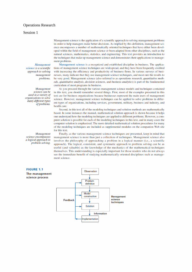
The simplex method uses an approach that is very efficient. It does not compute the value of

the objective function at every point; instead, it begins with a corner point of the feasibility

region where all the main variables are zero and then systematically moves from corner point

to corner point, while improving the value of the objective function at each stage. The

process continues until the optimal solution is found.

To learn the simplex method, we try a rather unconventional approach. We first list the

algorithm, and then work a problem. We justify the reasoning behind each step during the

process. A thorough justification is beyond the scope of this course.

We start out with an example we solved in the last chapter by the graphical method. This will

provide us with some insight into the simplex method and at the same time give us the chance

to compare a few of the feasible solutions we obtained previously by the graphical method.

But first, we list the algorithm for the simplex method.

Session 7 to 10

VAM

HAM

Assignment problem Hungarian method example

An assignment problem can be easily solved by applying Hungarian method which consists

of two phases. In the first phase, row reductions and column reductions are carried out. In the

second phase, the solution is optimized on iterative basis.

Phase 1

Step 0: Consider the given matrix.

Step 1: In a given problem, if the number of rows is not equal to the number of columns and

vice versa, then add a dummy row or a dummy column. The assignment costs for dummy

cells are always assigned as zero.

Step 2: Reduce the matrix by selecting the smallest element in each row and subtract with

other elements in that row.

Phase 2:

Step 3: Reduce the new matrix column-wise using the same method as given in step 2.

Step 4: Draw minimum number of lines to cover all zeros.

Step 5: If Number of lines drawn = order of matrix, then optimally is reached, so proceed to

step 7. If optimally is not reached, then go to step 6.

Step 6: Select the smallest element of the whole matrix, which is NOT COVERED by lines.

Subtract this smallest element with all other remaining elements that are NOT COVERED by

lines and add the element at the intersection of lines. Leave the elements covered by single

line as it is. Now go to step 4.

Step 7: Take any row or column which has a single zero and assign by squaring it. Strike off

the remaining zeros, if any, in that row and column (X). Repeat the process until all the

assignments have been made.

Step 8: Write down the assignment results and find the minimum cost/time.

Note: While assigning, if there is no single zero exists in the row or column, choose any one

zero and assign it. Strike off the remaining zeros in that column or row, and repeat the same

for other assignments also. If there is no single zero allocation, it means multiple numbers of

solutions exist. But the cost will remain the same for different sets of allocations.

Session 11 to 14

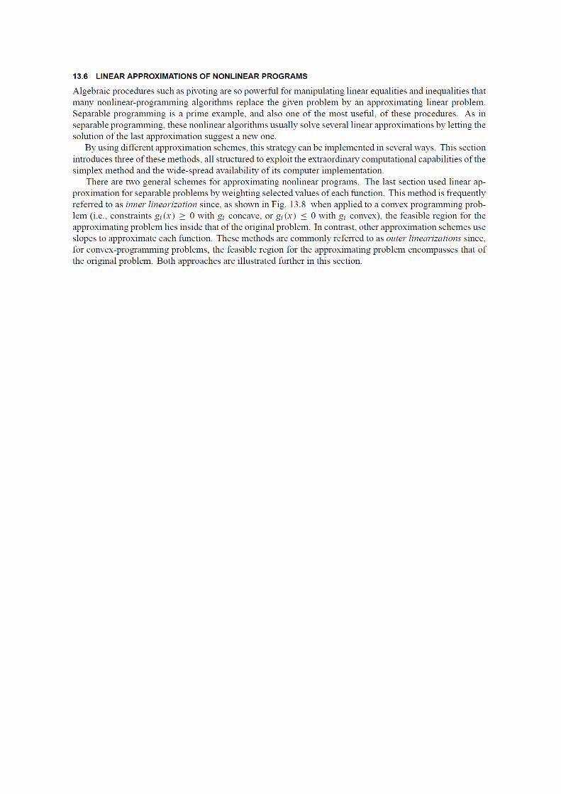
Nonlinear programming

Introduction

You will recall that in formulating linear programs (LP's) and integer programs

(IP's) we tried to ensure that both the objective and the constraints were linear -

that is each term was merely a constant or a constant multiplied by an unknown

(e.g. 5x is a linear term but 5x² a nonlinear term). Unless all terms were linear our

solution algorithms (simplex/interior point for LP and tree search for IP) would not

work.

Here we will look at problems which do contain nonlinear terms. Such problems

are generally known as nonlinear programming (NLP) problems and the entire

subject is known as nonlinear programming.

Session 15 to 17

What Is Game Theory?

Game theory is a theoretical framework for conceiving social situations among competing

players. In some respects, game theory is the science of strategy, or at least the optimal

decision-making of independent and competing actors in a strategic setting.

The key pioneers of game theory were mathematician John von Neumann and economist

Oskar Morgenstern in the 1940s. Mathematician John Nash is regarded by many as providing

the first significant extension of the von Neumann and Morgenstern work.

KEY TAKEAWAYS

Game theory is a theoretical framework to conceive social situations among

competing players and produce optimal decision-making of independent and

competing actors in a strategic setting.

Using game theory, real-world scenarios for such situations as pricing competition

and product releases (and many more) can be laid out and their outcomes predicted.

Scenarios include the prisoner's dilemma and the dictator game among many others.

The Basics of Game Theory

The focus of game theory is the game, which serves as a model of an interactive situation

among rational players. The key to game theory is that one player's payoff is contingent on

the strategy implemented by the other player. The game identifies the players' identities,

preferences, and available strategies and how these strategies affect the outcome. Depending

on the model, various other requirements or assumptions may be necessary.

Game theory has a wide range of applications, including psychology, evolutionary biology,

war, politics, economics, and business. Despite its many advances, game theory is still a

young and developing science.

Game Theory Definitions

Any time we have a situation with two or more players that involve known payouts or

quantifiable consequences, we can use game theory to help determine the most likely

outcomes. Let's start out by defining a few terms commonly used in the study of game theory:

Game: Any set of circumstances that has a result dependent on the actions of two or

more decision-makers (players)

Players: A strategic decision-maker within the context of the game

Strategy: A complete plan of action a player will take given the set of circumstances

that might arise within the game

Payoff: The payout a player receives from arriving at a particular outcome (The

payout can be in any quantifiable form, from dollars to utility.)

Information set: The information available at a given point in the game (The

term information set is most usually applied when the game has a sequential

component.)

Equilibrium: The point in a game where both players have made their decisions and

an outcome is reached

The Nash Equilibrium

Nash Equilibrium is an outcome reached that, once achieved, means no player can increase

payoff by changing decisions unilaterally. It can also be thought of as "no regrets," in the

sense that once a decision is made, the player will have no regrets concerning decisions

considering the consequences.

The Nash Equilibrium is reached over time, in most cases. However, once the Nash

Equilibrium is reached, it will not be deviated from. After we learn how to find the Nash

Equilibrium, take a look at how a unilateral move would affect the situation. Does it make

any sense? It shouldn't, and that's why the Nash Equilibrium is described as "no regrets."

Generally, there can be more than one equilibrium in a game.

However, this usually occurs in games with more complex elements than two choices by two

players. In simultaneous games that are repeated over time, one of these multiple equilibria is

reached after some trial and error. This scenario of different choices overtime before reaching

equilibrium is the most often played out in the business world when two firms are

determining prices for highly interchangeable products, such as airfare or soft drinks.

Impact on Economics and Business

Game theory brought about a revolution in economics by addressing crucial problems in prior

mathematical economic models. For instance, neoclassical economics struggled to understand

entrepreneurial anticipation and could not handle the imperfect competition. Game theory

turned attention away from steady-state equilibrium toward the market process.

In business, game theory is beneficial for modeling competing behaviors between economic

agents. Businesses often have several strategic choices that affect their ability to realize

economic gain. For example, businesses may face dilemmas such as whether to retire existing

products or develop new ones, lower prices relative to the competition, or employ new

marketing strategies. Economists often use game theory to understand oligopoly firm

behavior. It helps to predict likely outcomes when firms engage in certain behaviors, such as

price-fixing and collusion.

Types of Game Theory

Although there are many types (e.g., symmetric/asymmetric, simultaneous/sequential, et al.)

of game theories, cooperative and non-cooperative game theories are the most

common. Cooperative game theory deals with how coalitions, or cooperative groups, interact

when only the payoffs are known. It is a game between coalitions of players rather than

between individuals, and it questions how groups form and how they allocate the payoff

among players.

Non-cooperative game theory deals with how rational economic agents deal with each other

to achieve their own goals. The most common non-cooperative game is the strategic game, in

which only the available strategies and the outcomes that result from a combination of

choices are listed. A simplistic example of a real-world non-cooperative game is Rock-Paper-

Scissors.

Examples of Game Theory

There are several "games" that game theory analyzes. Below, we will just briefly describe a

few of these.

The Prisoner's Dilemma

The Prisoner's Dilemma is the most well-known example of game theory. Consider the

example of two criminals arrested for a crime. Prosecutors have no hard evidence to convict

them. However, to gain a confession, officials remove the prisoners from their solitary cells

and question each one in separate chambers. Neither prisoner has the means to communicate

with each other. Officials present four deals, often displayed as a 2 x 2 box.

1. If both confess, they will each receive a five-year prison sentence.

2. If Prisoner 1 confesses, but Prisoner 2 does not, Prisoner 1 will get three years and

Prisoner 2 will get nine years.

3. If Prisoner 2 confesses, but Prisoner 1 does not, Prisoner 1 will get 10 years, and

Prisoner 2 will get two years.

4. If neither confesses, each will serve two years in prison.

5. The most favorable strategy is to not confess. However, neither is aware of the other's

strategy, and without certainty that one will not confess, both will likely confess and

receive a five-year prison sentence. The Nash equilibrium suggests that in a prisoner's

dilemma, both players will make the move that is best for them individually but worse

for them collectively.

6. The expression "tit for tat" has been determined to be the optimal strategy for

optimizing a prisoner's dilemma. Tit for tat was introduced by Anatol Rapoport, who

developed a strategy in which each participant in an iterated prisoner's dilemma

follows a course of action consistent with his opponent's previous turn. For example,

if provoked, a player subsequently responds with retaliation; if unprovoked, the player

cooperates.

Dictator Game

This is a simple game in which Player A must decide how to split a cash prize with Player B,

who has no input into Player A’s decision. While this is not a game theory strategy per se, it

does provide some interesting insights into people’s behavior. Experiments reveal about 50%

keep all the money to themselves, 5% split it equally, and the other 45% give the other

participant a smaller share.

The dictator game is closely related to the ultimatum game, in which Player A is given a set

amount of money, part of which has to be given to Player B, who can accept or reject the

amount given. The catch is if the second player rejects the amount offered, both A and B get

nothing. The dictator and ultimatum games hold important lessons for issues such as

charitable giving and philanthropy.

Volunteer’s Dilemma

In a volunteer’s dilemma, someone has to undertake a chore or job for the common good. The

worst possible outcome is realized if nobody volunteers. For example, consider a company in

which accounting fraud is rampant, though top management is unaware of it. Some junior

employees in the accounting department are aware of the fraud but hesitate to tell top

management because it would result in the employees involved in the fraud being fired and

most likely prosecuted.

Being labeled as a whistleblower may also have some repercussions down the line. But if

nobody volunteers, the large-scale fraud may result in the company’s

eventual bankruptcy and the loss of everyone’s jobs.

The Centipede Game

The centipede game is an extensive-form game in game theory in which two players

alternately get a chance to take the larger share of a slowly increasing money stash. It is

arranged so that if a player passes the stash to his opponent who then takes the stash, the

player receives a smaller amount than if he had taken the pot.

The centipede game concludes as soon as a player takes the stash, with that player getting the

larger portion and the other player getting the smaller portion. The game has a pre-defined

total number of rounds, which are known to each player in advance.

Limitations of Game Theory

The biggest issue with game theory is that, like most other economic models, it relies on the

assumption that people are rational actors that are self-interested and utility-maximizing. Of

course, we are social beings who do cooperate and do care about the welfare of others, often

at our own expense. Game theory cannot account for the fact that in some situations we may

fall into a Nash equilibrium, and other times not, depending on the social context and who the

players are.

What are the 'games' being played in game theory?

It is called game theory since the theory tries to understand the strategic actions of two or

more "players" in a given situation containing set rules and outcomes. While used in a

number of disciplines, game theory is most notably used as a tool within the study of business

and economics. The "games" may thus involve how two competitor firms will react to price

cuts by the other, if a firm should acquire another, or how traders in a stock market may react

to price changes.

In theoretic terms, these games may be categorized as similar to prisoner's dilemmas, the

dictator game, the hawk-and-dove, and battle of the sexes, among several other variations.

What are some of the assumptions about these games?

Like many economic models, game theory also contains a set of strict assumptions that must

hold for the theory to make good predictions in practice. First, all players are utility-

maximizing rational actors that have full information about the game, the rules, and the

consequences. Players are not allowed to communicate or interact with one another. Possible

outcomes are not only known in advance but also cannot be changed. The number of players

in a game can theoretically be infinite, but most games will be put into the context of only

two players.

What is a Nash equilibrium?

The Nash equilibrium is an important concept referring to a stable state in a game where no

player can gain an advantage by unilaterally changing a strategy, assuming the other

participants also do not change their strategies. The Nash equilibrium provides the solution

concept in a non-cooperative (adversarial) game. It is named after John Nash who received

the Nobel in 1994 for his work

Who came up with game theory?

Game theory is largely attributed to the work of mathematician John von Neumann and

economist Oskar Morgenstern in the 1940s, and was developed extensively by many other

researchers and scholars in the 1950s. It remains an area of active research and applied

science to this day.

Session 18 to 20

Session 21 to 24

Session 25 to 27

Session 28 to 30

Meaning of Markov Analysis:

Markov analysis is a method of analyzing the current behaviour of some variable in

an effort to predict the future behaviour of the same variable. This procedure was

developed by the Russian mathematician, Andrei A. Markov early in this century. He

first used it to describe and predict the behaviour of particles of gas in a closed

container. As a management tool, Markov analysis has been successfully applied to a

wide variety of decision situations.

Perhaps its widest use is in examining and predicting the behaviour of customers in

terms of their brand loyalty and their switching from one brand to another. Markov

processes are a special class of mathematical models which are often applicable to

decision problems. In a Markov process, various states are defined. The probability

of going to each of the states depends only on the present state and is independent of

how we arrived at that state.

A simple Markov process is illustrated in the following example:

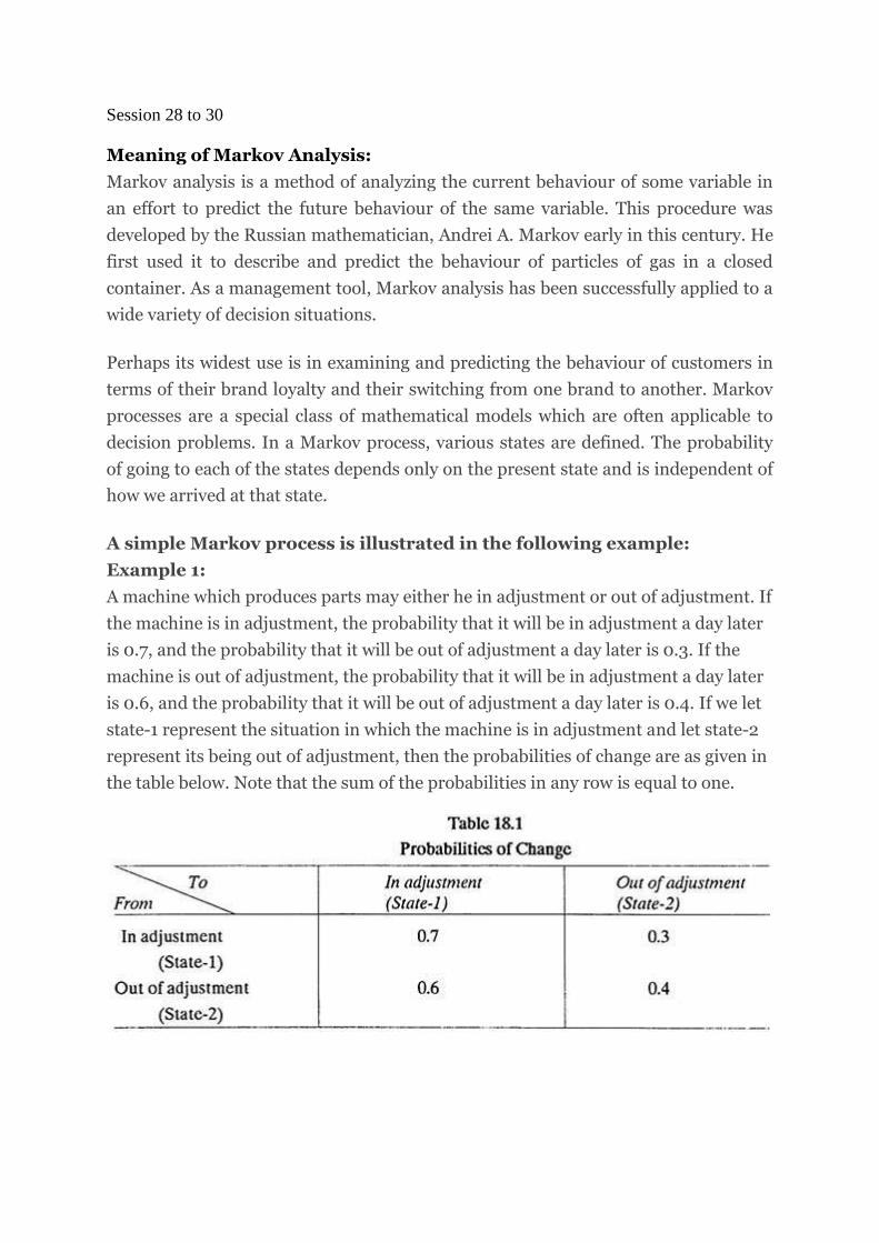
Example 1:

A machine which produces parts may either he in adjustment or out of adjustment. If

the machine is in adjustment, the probability that it will be in adjustment a day later

is 0.7, and the probability that it will be out of adjustment a day later is 0.3. If the

machine is out of adjustment, the probability that it will be in adjustment a day later

is 0.6, and the probability that it will be out of adjustment a day later is 0.4. If we let

state-1 represent the situation in which the machine is in adjustment and let state-2

represent its being out of adjustment, then the probabilities of change are as given in

the table below. Note that the sum of the probabilities in any row is equal to one.

Solution:

The process is represented in Fig. 18.4 by two probability trees whose upward

branches indicate moving to state-1 and whose downward branches indicate moving

to state-2.

Suppose the machine starts out in state-1 (in adjustment), Table 18.1 and Fig.18.4

show there is a 0.7 probability that the machine will be in state-1 on the second day.

Now, consider the state of machine on the third day. The probability that the

machine is in state-1 on the third day is 0.49 plus 0.18 or 0.67 (Fig. 18.4).

The corresponding probability that the machine will be in state-2 on day 3, given that

it started in state-1 on day 1, is 0.21 plus 0.12, or 0.33. The probability of being in

state-1 plus the probability of being in state-2 add to one (0.67 + 0.33 = 1) since there

are only two possible states in this example.

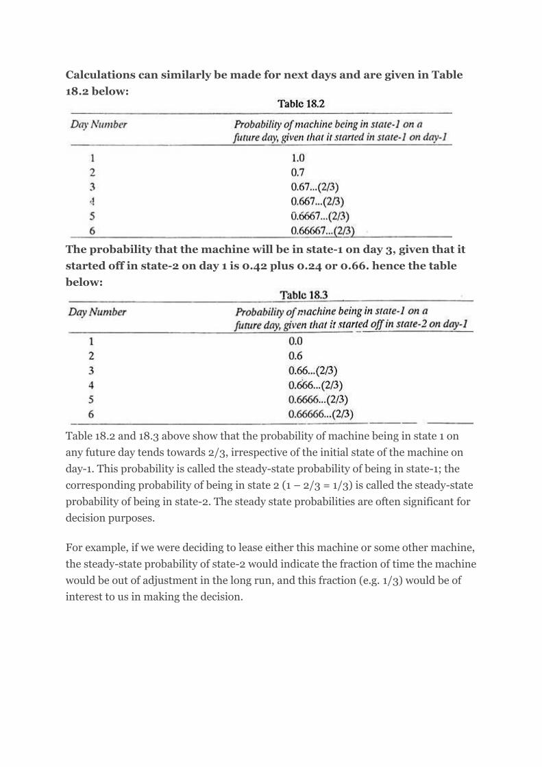
Calculations can similarly be made for next days and are given in Table

18.2 below:

The probability that the machine will be in state-1 on day 3, given that it

started off in state-2 on day 1 is 0.42 plus 0.24 or 0.66. hence the table

below:

Table 18.2 and 18.3 above show that the probability of machine being in state 1 on

any future day tends towards 2/3, irrespective of the initial state of the machine on

day-1. This probability is called the steady-state probability of being in state-1; the

corresponding probability of being in state 2 (1 – 2/3 = 1/3) is called the steady-state

probability of being in state-2. The steady state probabilities are often significant for

decision purposes.

For example, if we were deciding to lease either this machine or some other machine,

the steady-state probability of state-2 would indicate the fraction of time the machine

would be out of adjustment in the long run, and this fraction (e.g. 1/3) would be of

interest to us in making the decision.

Markov analysis has come to be used as a marketing research tool for examining and

forecasting the frequency with which customers will remain loyal to one brand or

switch to others. It is generally assumed that customers do not shift from one brand

to another at random, but instead will choose to buy brands in the future that reflect

their choices in the past.

Other applications that have been found for Markov Analysis include the

following models:

A model for manpower planning,

A model for human needs,

A model for assessing the behaviour of stock prices,

A model for scheduling hospital admissions,

A model for analyzing internal manpower supply etc.