OPTICAL BUSES

CSC 8530 : Parallel AlgorithmInstructor : Dr. Sushil PrasadPresented by : DM Rasanjalee Himali

OVERVIEW

• Introduction to Optical Buses

• Linear Array of Optical Buses– Waiting Function– Two-Way Communication

• Data Communication– Broadcasting– Permutation – Data Distribution

• PRAM Simulation

• Meshes with Optical Buses

• Paper

BUS

• Bus : – a communication link to some/all of the processors in mesh– can be used for direct communication between non-neighboring

processors– Traditionally was electronic– Broadcasting has exclusive access to bus

• Properties:1. The bidirectionality

– Datum placed on bus by processor P travels on the bus in both directions (left, right) simultaneously reaching all processors attached to the bus

2. The lack of a precise function describing time taken by signal to propagate along given section of a wire– Assume O(1) time

OPTICAL BUSES

• Alternative to electronic buses• Uses light signals• Bus is called an optical waveguide• Allows several processors to inject data on to the bus

simultaneously– Each datum destined for one or several processors

• Properties:1. Unidirectionality

– Datum placed on bus travel in only one (always the same) direction

2. Predictability of propagation delay per unit time is linear• Time taken to travel distance

OPTICAL BUSES

• Let processors P0, P1…Pn-1 are connected to an optical bus

• Several processors can place data on the bus simultaneously, one datum per processor (property 1)

• Data form a pipeline and travel down the bus in the same direction

• Difference between arrival times of two data di and dj at a processor Pl can be determined by distances separating Pi and Pj (property 2)

P0 Pi Pj Pk Pl Pn-1

di dj dk

Optical Waveguide (bus)

A pipeline of data on an optical bus

LINEAR ARRAYS WITH OPTICAL BUSES• Processors are arranged in a 1-

dimensional pattern

• n processors are connected to an optical wave

• Each processor is attached to the bus via a two-way link

– One to write data on to the bus– Other to read data from the bus

• No processor is directly connected to another processor by a standard linear-array link

• • Unidirectional bus:

– Pi can send message to Pj if j>i

A linear array of data with an optical bus

P0 Pi Pn-1

D

write

rea

d

LINEAR ARRAYS WITH OPTICAL BUSES

• Let ,– b :bits per datum/message placed on bus

– w : width of light pulse representing the bit• duration of pulse in time units

– Optical Distance between any two processors Pi and Pj is:

• the length of waveguide separating them

– D : optical distance between any two consecutive processors• Is a constant

D :number of time units required by a light pulse to traverse D D = D / v

• v : speed of light

• If Pi sends message to Pj (j>i), message arrives at Pj after (j-i) D time units

LINEAR ARRAYS WITH OPTICAL BUSES

• All processors can place data on bus simultaneously– This leads to overlapping of messages

• To avoid message overlap the following conditions must be satisfied1. D > bwv2. Processors wishing to write on the bus do so synchronously

– They place data on the bus at pre-specified times, separated by regular time intervals

• Bus Cycle : B(L) : time taken by an optical signal to traverse the optical bus from one end(P0) to

the other (P n-1) – = O(1)– Assume B(L) smaller than or equal to the time required by a basic computational

operations

• Optical length of bus L:– L = (n-1)D

B(L) = L/v• Time is divided into bus cycle intervals

LINEAR ARRAYS WITH OPTICAL BUSES

• Waiting function:– When is a processor Pj to read a message di

from the bus?

– Two cases:

1. Receiver Pj knows the identity of the sender Pi

2. Receiver Pj does not know the identity of the sender Pi

WAITING FUNCTION

1. Receiver Pj knows the identity of the sender Pi

• All processors wishing to place a datum on the bus do so only at the beginning of a bus cycle before reading di

• Function : wait(i,j):– Definition 1:

• wait(i,j) = (j - i) D = (j – i) ; D = o(1)

– Definition 2:• If , during each bus cycle, each processor is required to place a

message on the bus:

• wait(i,j) – 1 gives the no. of messages P j should skip before reading d i

• Transmission of di from Pi to Pj takes one bus cycle

LINEAR ARRAYS WITH OPTICAL BUSES

1. Receiver Pj knows the identity of the sender Pi

• EXAMPLE :

• n = 5

• P3 expects d0 (from P0)

• P4 expects d2 (from P2)

• Relative to the beginning of the bus cycle,– P0 and P2 place data at the

beginning of the bus cycle

– P4 receives d2 at time 4-2 =2

– P3 receives d0 at time 3-0 =3

A linear array of data with an optical bus

P0 P1 P4

d0 d2

P2 P3

T = 0 T = 1 T = 2 T = 3 T = 4

d0 d2

LINEAR ARRAYS WITH OPTICAL BUSES

2. Receiver Pj does not knows the identity of the sender Pi

• But the sender knows the identity of the receiver

• Sender Pi writes message di destined to Pj, on the bus at time ((n-1)-j+i)D relative to the beginning of bus cycle

• All processors read the bus simultaneously at the end of the bus cycle (at time (n-1)D )

• Transmission of di from Pi to Pj takes one bus cycle

LINEAR ARRAYS WITH OPTICAL BUSES

1. Receiver Pj does not know the identity of the sender Pi

• EXAMPLE :

• n = 5

• P0 wish to send d0 (to P3)

• P2 wish to send d2 (to P4)

• Relative to the beginning of the bus cycle,– Place data at time :((n-1)-j+i)

– P0 place d0 at time (5-1)-3+0 =2

– P2 place d2 at time (5-1)-4+2 =3

– Data reach destination at time 4

A linear array of data with an optical bus

P0 P1 P4

d0 d2

P2 P3

T = 0 T = 1 T = 2 T = 3 T = 4

d0 d2

LINEAR ARRAYS WITH OPTICAL BUSES

• Two Way Communication• Allows messages to be sent in both

directions

• Two optical buses used– Upper bus: send data L R– Lower bus: send data R L

• Wait function:

P0 Pi Pn-1

If wait(i,j)>0 thenPj reads di from the upper bus at time wait(i,j)

Else If wait(i,j) < 0 thenPj reads di from the lower bus at time –wait(i,j)

ElsePj does not read in this cycle

End If

DATA COMMUNICATION

• Linear array with optical buses can be used to execute a variety of data communication schemes.

• Ex:– Broadcasting– Permutation– Data Distribution

• All schemes are uniquely determined by the wait function

• We can define a communication pattern simply by giving wait function:– wait(i,j) = j – i

BROADCASTING

• Processor Pi wishes to broadcast a datum to all other processors

• Set wait(i,j) = j – i , for specific i and all j i

• Ex: – n =5– At beginning of bus cycle P2 place d2

on both upper and lower buses– Datum reach P1 and P3

simultaneously– Then it reaches P0 and P4

simultaneously

• Broadcast takes one bus cycle

P0 P1 P4P2 P3

T=0 T=1 T=2 T=3 T=4

d2

d2

d2 d2d2d2

PERMUTATION

• Arbitrary permutation r of indices {0,1,…,n-1}

– 0 <= i, r(i) <= n-1– di is sent to Pr(i) for every i– Each processor receives exactly 1 datum

• Ex:– n = 5– Pi holds di for 0<=i<=n-1– Permutation needed:

• P0 hold d4,• P1 hold d3• P2 hold d1• P3 hold d0• P4 hold d2

– Initially each processor places its data on upper and lower waveguides at beginning of bus cycle

– Entire permutation takes one bus cycle

P0 P1 P4P2 P3

T=0 T=1 T=2 T=3 T=4

d2

d1

d0

d3d4

d1 d2d3 d0d4

DATA DISTRIBUTION

• Send datum di held by Pi to two or more processors or no processors at all

• s(j) : index of the processor from which Pj receives a datum where 0 <= j,s(j) <= n-1

• This allows s(j) = s(k) = I for j k– Function is not necessarily a permutation

• Set wait(s(j),j) = j – s(j) , for all j• Ex:

– n =5– Pi holds di for 0 <= I <= n-1– Distribution needed:’

• P0 hold d3,• P1 hold d3• P2 hold d0• P3 hold d1• P4 hold d0

– Performed in same way as permutation– Entire distribution takes one bus cycle

PRAM SIMULATION

• Broadcasting, permutation and distribution takes 1 bus cycle (O(1) time)

• Permutation and data distribution allow a linear array of n processors with optical buses and O(1) memory locations per processor to simulate in constant time any form of memory access allowed on a PRAM with n processors and O(n) shared memory locations (except CW operation)

• ER and EW are permutations of the data• CR is a data distribution operation• CW cannot be simulated in constant time

B(L) is assumed to be smaller than or equal to time required by a basic operation

– but CW typically involves arbitrary no. of such operations.

MESHES WITH OPTICAL BUSES

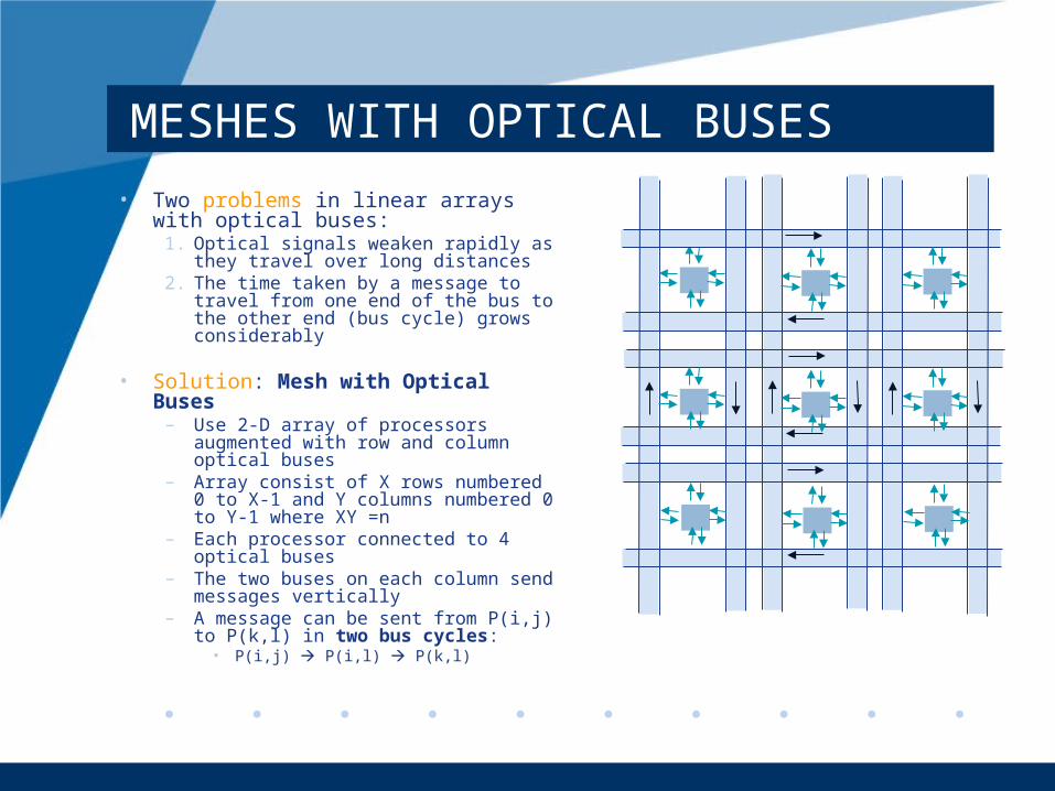
• Two problems in linear arrays with optical buses:

1. Optical signals weaken rapidly as they travel over long distances

2. The time taken by a message to travel from one end of the bus to the other end (bus cycle) grows considerably

• Solution: Mesh with Optical Buses– Use 2-D array of processors

augmented with row and column optical buses

– Array consist of X rows numbered 0 to X-1 and Y columns numbered 0 to Y-1 where XY =n

– Each processor connected to 4 optical buses

– The two buses on each column send messages vertically

– A message can be sent from P(i,j) to P(k,l) in two bus cycles:

• P(i,j) P(i,l) P(k,l)

PARALLEL ALGORITHMS AND ARCHITECTURES BASED ON PIPELINED OPTICAL BUSES

• Purpose of the paper:– Explore potential value of a

new kind of an optical bus for SIMD architectures in which processing units are connected with buses

• Two basic multiprocessor interconnection schemes:– Nearest-neighbor connection

– Exclusive-access bus connection

PARALLEL ALGORITHMS AND ARCHITECTURES BASED ON PIPELINED OPTICAL BUSES

• Each scheme has both advantages and disadvantages.

• nearest-neighbor connection– There can be O(n) active messages in the system at

any time instant– But takes up to O(n) steps to have a message

delivered from one processor to another.

• exclusive-access bus connection– Any message transfer takes only one step (one bus

Cycle– Because the access of the bus by processors is

exclusive there can be only one active message on the bus at any time.

• To obtain a high communication efficiency it is desirable to combine the advantages of the two interconnections

– allowing both O(n) active messages at any time and a one-step message transfer between any two processors.

– This may be achieved by the use of a message-pipelined optical bus

PIPELINED OPTICAL BUS

• The pipelined optical bus takes advantage of two unique properties of optical signal transmissions in waveguides:– unidirectional propagation and – predictable path delays.

• Each processor is coupled to the optical bus waveguide with two passive optical couplers, one for writing signals, and the other for reading.

• All the processors may write their messages on an optical bus simultaneously

PIPELINED OPTICAL BUS

• To be able to transmit messages in both directions in the same bus cycle, a second bus can be added. Then we obtain the architecture of a linear array processor with pipelined buses (APPB) with dual-bus connections in which each processor is coupled to two optical buses, one for message transfers in each direction:

APPB WITH FOLDED OPTICAL BUS

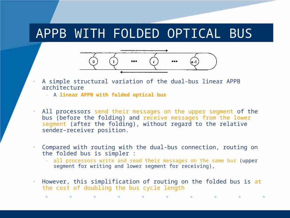
• A simple structural variation of the dual-bus linear APPB architecture– A linear APPB with folded optical bus

• All processors send their messages on the upper segment of the bus (before the folding) and receive messages from the lower segment (after the folding), without regard to the relative sender–receiver position.

• Compared with routing with the dual-bus connection, routing on the folded bus is simpler :

– all processors write and read their messages on the same bus (upper segment for writing and lower segment for receiving),

• However, this simplification of routing on the folded bus is at the cost of doubling the bus cycle length

APPB WITH FOLDED OPTICAL BUS

• dual-bus connections: wait takes both positive and negative values,

• Folded bus : wait is always positive

• The linear APPB architectures can be extended to 2-D APPB’s in which processors in each row and column may be connected with either dual or folded buses.

INTEGER ADDITION

• Add two n-bit integers x = xn-1…x0 and y = yn-1…y0

• Let – sum z = znzn-1…z0

– Carry-in ci = carry in at the ith bit ; c0 =0

• If ci is known, then xi+yi+ci can be calculated

• zi and ci+1(carry-out at bit i) are equal to the lower and higher bits of the sum respectively

• Using one processor, we can compute xi+yi+ci to obtain zi and ci+1 sequentially for i=0,1,…,n-1 and finish addition in O(n) steps

• With carry look-ahead addition, the computation can be completed in faster in optical bus

CARRY LOOK-AHEAD ADDITION

• Carry look-ahead logic uses the concepts of generating and propagating carries

• The addition of two bits A and B is said to generate if the addition will always carry, regardless of whether there is an input carry

– Gi = Ai.Bi

• A + B is said to propagate if the addition will carry whenever there is an input carry

– Pi = Ai Bi

CARRY LOOK-AHEAD ADDITION

• For each bit in a binary sequence to be added, the Carry Look Ahead Logic will determine whether that bit pair will generate a carry or propagate a carry.

• This allows the circuit to "pre-process" the two numbers being added to determine the carry ahead of time.

• Then, when the actual addition is performed, there is no delay from waiting for the ripple carry effect (or time it takes for the carry from the first Full Adder to be passed down to the last Full Adder)

INTEGER ADDITION

• With folded optical bus, carry look-ahead addition can be performed in O(1) steps.

• Number of processors required : n+1

• ci can be determined quickly by the examination of a string of g,s and p obtained at bit positions lower than i – g is assigned to bit i if xi = yi = 1

• This is because a carry-out is always generated at this bit position, regardless of the value of the carry-out from the lower bits

– s is assigned to bit i if xi = yi = 0• This is because the carry-out from lower bits is stopped at this point

– p is assigned to bit i if xi yi • This is because carry out from lower bit is propagated through this bit

INTEGER ADDITION

• Ex: g-s-p string for addition of two 12- bit numbers– g is assigned to bit i if xi = yi = 1

– s is assigned to bit I if xi = yi = 0

– p is assigned to bit I if xi yi

• The g, s, and p values can be represented with a 2-bit variable, Ai, at each processor i.

INTEGER ADDITION

• Let k be the largest index smaller than i such that Ak p.

• Then it is easy to show that ci =1 iff Ak =g.

• Therefore we have the following algorithm for computing the addition:– In the algorithm it is assumed that initially xi and yi are held by processor i.

– At the completion of the algorithm, zi is stored at processor i.

REFERENCES

• Akl, Parallel Computation, Models and Methods, Prentice Hall 1997

• Parallel algorithms and architectures based on pipelined optical buses, Zicheng Guo and H. John Caulfield, APPLIED OPTICS ,Optical Society of America, Vol. 34, No. 35 , 10 December 1995