Journal of Graph Algorithms and Applicationshttp://jgaa.info/ vol. 17, no. 4, pp. 541–565 (2013)DOI: 10.7155/jgaa.00303

Optical Graph Recognition

Christopher Auer 1 Christian Bachmaier 1 Franz J. Brandenburg 1

Andreas Gleißner 1 Josef Reislhuber 1

1University of Passau, 94030 Passau, Germany

Abstract

Optical graph recognition (OGR) reverses graph drawing. A drawingtransforms the topological structure of a graph into a graphical represen-tation. Primarily, it maps vertices to points and displays them by icons,and it maps edges to Jordan curves connecting the endpoints.OGR transforms the digital image of a drawn graph into its topologicalstructure. It consists of four phases, preprocessing, segmentation, topol-ogy recognition, and postprocessing. OGR is based on established digitalimage processing techniques. Its novelty is the topology recognition wherethe edges are recognized with emphasis on the attachment to their verticesand on edge crossings.

Our prototypical implementation OGRup shows the effectiveness ofthe approach and produces a GraphML file, which can be used for furtheralgorithmic studies and graph drawing tools. It has been tested both onhand-made graph drawings and on drawings generated by graph drawingalgorithms.

Submitted:December 2012

Reviewed:February 2013

Revised:March 2013

Accepted:April 2012

Final:April 2012

Published:July 2013

Article type:Regular paper

Communicated by:W. Didimo and M. Patrignani

A preliminary version [2] appeared in the 20th Symposium on Graph Drawing GD 2012.E-mail addresses: auerc@fim.uni-passau.de (Christopher Auer) bachmaier@fim.uni-passau.de(Christian Bachmaier) brandenb@fim.uni-passau.de (Franz J. Brandenburg) gleissner@fim.uni-passau.de (Andreas Gleißner) reislhuber@fim.uni-passau.de (Josef Reislhuber)

542 C. Auer et al. Optical Graph Recognition

1 Introduction

Graph drawing addresses the problem of constructing visualizations of graphs,networks and related structures. It adds geometric and graphic information, as-signing coordinates to the vertices and routing the edges, and attaches graphicfeatures such as icons, line styles and colors. The goal is a “nice” drawing,which shall convey the underlying structural relations and make them easilyunderstandable to a human user. “Nice” can be evaluated empirically and ap-proximated by formal terms, such as bends, crossings, angular resolution, anduniform distribution [14]. This is what the field of graph drawing is all about.

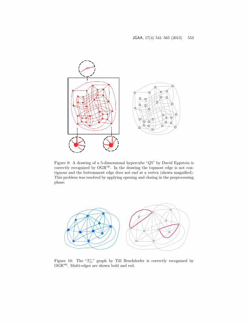
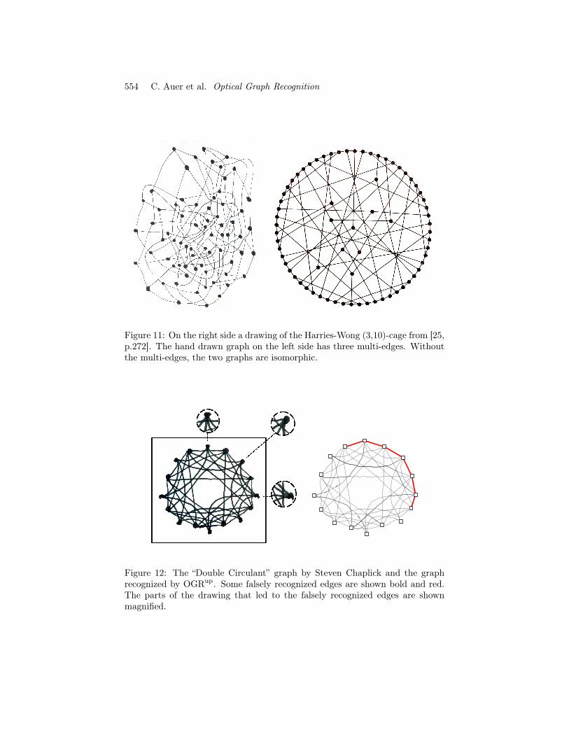
The reverse process has been neglected so far. There is a need for it. Weoften make drafts of a diagram using pencil and paper and then would like to usea graph drawing tool for improvements of the drawing or a graph algorithm foran analysis. For instance, Fig. 11 shows a hand-made drawing of a graph thatcontains three multi-edges. Without the multi-edges, the graph is isomorphicto the Harries-Wong (3,10)-cage. However, for a human this is hard to verify.Here optical graph recognition comes into play. One needs a tool to convert theimage of a drawn graph into the topological structure. At the 20th Symposiumon Graph Drawing (GD 2012) in Redmond, WA we have asked ten participantsto draw a graph by hand. On the spot, our prototype for graph recognitionOGRup correctly recognized five graphs. Two correctly recognized examplesare shown in Figs. 9 and 10. Both graphs support our motivation for opticalgraph recognition as they have graph theoretic properties which are difficult tocheck for a human, but can be easily validated by an analysis tool. Figure 9 (byDavid Eppstein) shows a 5-dimensional hypercube which is missing four edgesin the upper-leftmost part of the drawing and Fig. 10 (by Till Bruckdorfer) hasmulti-edges. One of the five drawings that were not correctly recognized, is the“Double Circulant” graph (by Steven Chaplick) in Fig. 12. OGRup recognizedsome edges as incident to a vertex, although they pass the vertex. A human willcorrectly recognize the graph using the context information “Double Circulant”and will infer that two neighboring vertices on the circle are not adjacent.

In this paper, we propose optical graph recognition (OGR) as a method toautomatically extract the topological structure of a graph from its drawing.OGR is an adaption of optical character recognition (OCR) [7], which extractsplain text from images for automatic processing. Since there is a large variety,we restrict ourselves to the most common drawing types. The vertices are rep-resented by geometric objects such as circles or rectangles, which are connectedby (images of) Jordan curves representing the edges. The drawing is given asa (digital) image, see Fig. 2. OGR proceeds in four phases: preprocessing, seg-mentation, topology recognition, and postprocessing. The topology recognitionis the core of OGR. This phase takes a digital image as input, where all pixelsare classified as either background, vertex, or edge pixels. In the image, theregions of vertex pixels of two vertices are connected by a contiguous region ofedge pixels if the two vertices are connected by an edge. However, the converseis not true. A contiguous region of edge pixels corresponds to several edges ifthe edges cross, see Fig. 2 and the left part of Fig. 6. The problem of crossing

JGAA, 17(4) 541–565 (2013) 543

edges does not occur if the drawing is plane. In this case there are approachesto recognize a planar graph [5] and to extract the circuit from its plane draw-ing [8, p. 476]. However, crossings are unavoidable. Our topology recognitionresolves crossings similarly to the human eye. The eye follows the edge curveto the crossing and then proceeds in the “most likely” direction, which is thedirection in which the edge curve enters the crossing.

Due to this similarity, OGR’s recognition rate can be used as a measure ofthe legibility of a drawing. OGR is error-prone if many edges cross at the samepoint or if edges cross in small angles. Such drawings are hardly legible forhumans as well [20,22]. Recently, Pach [24] defined unambiguous bold drawings,which leave no room for different interpretations of the topology of the graph.For example, in unambiguous drawings areas of overlapping edges do not hidevertices. In fact, OGR presumes an unambiguous bold drawing as input.

The problem of automatically recognizing objects has been studied exten-sively in the field of digital image processing. Most prominently, optical charac-ter recognition has significantly advanced in the last decades [7]. However, theemphasis behind OCR is to recognize the shape of a certain character ratherthan its topological structure as in OGR. In [11,23], the authors have proposedmethods to trace blood vessels and measure their size in X-ray images. Again,these approaches are designed to evaluate the shape of the blood vessels andignore their topological structure. During the past decade an increasing num-ber of research emerged at the intersection of pattern recognition and imageanalysis on one hand and graph theory on the other hand. In fact, the IAPRWorkshop on Graph-based Representations in Pattern Recognition is devotedto this topic.

Our paper is organized as follows. In Sect. 2, we give some preliminaries.The four-phases approach of OGR is presented in Sect. 3 with an emphasis onthe topology recognition phase in Sect. 3.3. An experimental evaluation is givenin Sect. 4 and we discuss “good” and “bad” features of a drawing for OGRup’srecognition rate.

2 PreliminariesIn this paper, we deal with undirected graphs G = (V,E). Directions of edgescan be recognized in a postprocessing phase of OGR. In the following, a drawingof G maps vertices to graphical objects like discs, rectangles, or other shapesin the plane. The edges are mapped to Jordan curves connecting its endpoints.For convenience, we speak of vertices and edges when they are elements of agraph, of its drawing, and in a digital image of the drawing. A port is the pointof an edge which meets the vertex. Each edge has exactly two ports. Note thatthis is only true if no edge crosses a vertex. In that case it is also hard for ahuman to recognize the adjacency correctly. Hence, we assume no edge-vertex-crossings in the following. An (edge-edge-)crossing is a point where two or moreedges cross.

544 C. Auer et al. Optical Graph Recognition

1 1 1

1

1

1 1

1 1

x

y

0

1

2

.

.

h

0 1 2 . . wx

y

0

1

2

.

.

h

0 1 2 . . w

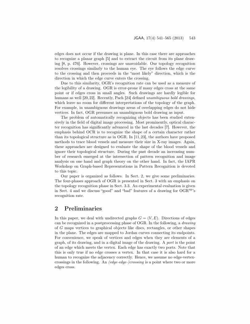
Figure 1: Erosion: The reference pixel (center) of the pattern (above the arrow)is put on every pixel of the image and if the pattern and the pixels underneathdo not match, the pixel underneath the center is turned into a background pixel.

A digital image is a set of pixels. Each pixel p has coordinates (x, y) in a two-dimensional grid of a certain width and height, and a color which is taken froma finite set C. In a binary image only two colors are allowed, i. e., C = {0, 1},where a pixel with color 0 is a background pixel (black) and a pixel with color1 is an object pixel (white). When a (color) image is converted into a binaryimage, the result is called binarized image.

The 4-neighborhood N4(x, y) of a pixel (x, y) consists of (x− 1, y), (x+1, y),(x, y− 1), and (x, y+1). Two pixels p and q of the same color are 4-adjacent ifthey are 4-neighbors. A 4-path from pixel (v, w) to pixel (x, y) is a sequence ofdistinct pixels (x0, y0), (x1, y1), . . . , (xk, yk), where (x0, y0) = (v, w), (xk, yk) =(x, y) and pixels (xi−1, yi−1) and (xi, yi) are 4-adjacent for 1 ≤ i ≤ k. A subsetof pixels R is called a 4-region if there is a 4-path between every pixel p ∈ R andq ∈ R such that |R| is maximal. The 8-neighborhood N8(x, y) of (x, y) consistsof N4(x, y) and additionally the pixels (x ± 1, y ± 1). 8-adjacency, 8-path, and8-region are defined analogously.

We use morphological image processing to alter or analyze binary images.Its basis is set theory. Each morphological operation relies on the same basicconcept, which is to fit a predefined structuring element on every pixel of animage and to compare the set of pixels from the structuring element with the setof pixels that lies underneath the structuring element. A structuring elementis a pattern of object and background pixels and is most commonly a squareof size 3 × 3. For example, erosion converts each object pixel with at leastone background pixel in its 8-neighborhood into a background pixel, see Fig. 1.Similarly, dilatation converts each background pixel with at least one objectpixel in its 8-neighborhood into an object pixel.

3 Optical Graph Recognition

OGR is divided into the four phases: preprocessing, segmentation, topologyrecognition, and postprocessing. The input of the first phase is a drawing of

JGAA, 17(4) 541–565 (2013) 545

a graph G as a digital image. From an information theoretic point of view,the information contained in the digital image is reduced, until only the setsof vertices and edges remain. Thereby a digital image with a size of severalMB is reduced to a GraphML file of only a few kB. Each of the followingsections is devoted to a phase, its purpose, suggestions for possible algorithms,and a description of our prototypical implementation OGRup. All phases butthe topology recognition use standard image processing techniques for whichwe only demonstrate their effects. The reader is referred to the literature onimage processing, e. g., [19]. The characteristic of our approach is the topologyrecognition phase, which is therefore described in more detail as it involvesnon-standard techniques developed for the purpose of OGR.

3.1 Preprocessing

The purpose of the preprocessing phase is to separate the pixels belonging tothe background from the pixels of the drawn graph. The image is binarizedsuch that every object pixel is part of the drawing and every background pixelis not. Information is removed from the image if it is unimportant to OGR, suchas the color. This can be achieved with any binarization algorithm like global,adaptive or hysteresis thresholding [10,11,13,17,19]. The extent of informationthat is filtered depends both on the drawing of the graph and the tasks of thesubsequent phases of OGR.

In OGRup we use histogram based global thresholding for the binarization [19,p. 599]. With this method, each pixel with a color (gray value) greater than apredefined threshold is an object pixel and it is a background pixel, otherwise.The threshold color t can either be set manually, or it is automatically estimatedby using the gray-level histogram. Fig. 2 shows the effect of binarization.

After binarization, we additionally apply the noise reduction method from[19, p. 531] depending on the quality of the image. There are two types ofnoise. Isolated object pixels (white) called salt and isolated background pixels(black) called pepper. Both types of noise can be reduced by the opening andclosing operators. The opening operator first erodes i times and then dilatatesi times; closing does the same in inverse order. Opening generally smoothensthe border of a region of object pixels and eliminates thin protrusions and thussalt [19, p. 528]. Closing also smoothens the border of object pixel regionsand removes pepper. Closing also fuses narrow breaks, eliminates small holes,and fills gaps in the border of object pixel regions. This is important in thecontext of OGR. For instance, if an edge curve is not contiguous or there is agap between the edge curve and its attached vertices due to bad image quality,the edge cannot be recognized. Closing makes edges contiguous and fills smallgaps between edges and vertices. But the number of closings i must be chosenwith care since too many closing operations may attach a passing edge to a non-incident vertex or may introduce touching edges, which are then classified ascrossing edges. Experiments with values of i > 1 often lead to these undesiredresults, therefore we recommend using only a single closing operation. By asimilar reasoning more than one opening operation is not advisable.

546 C. Auer et al. Optical Graph Recognition

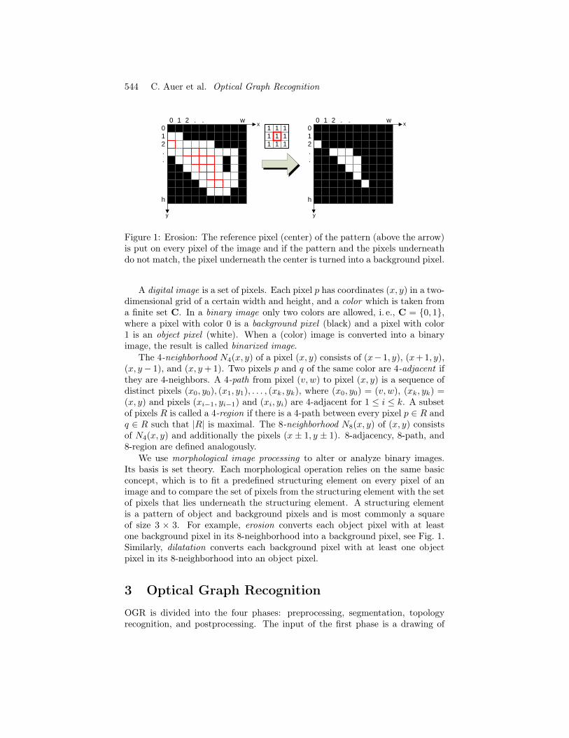
Figure 2: A drawing of a graph and the result of the preprocessing phase.

Figure 3: Vertex recognition in the segmentation phase: input, after erosion,and after dilatation.

3.2 Segmentation

The input of the segmentation phase is a binarized image resulting from thepreprocessing. In a nutshell, segmentation identifies the vertices in the binaryimage. More precisely, for each object pixel it determines whether it belongsto a vertex or to an edge. The output is a ternary image with three colors forbackground, vertex, and edge pixels. Note that, depending on the shape of thevertices, different methods have to be applied.

In OGRup, we have implemented a generic approach inspired by [8, p. 476]which assumes the following preconditions. The vertices are represented byfilled shapes, e. g., circles or rectangles, and the edges are represented by curvesof a width significantly smaller than the diameter of the vertices, see Fig. 3.Using this assumption, we can use the opening operator, which first erodes ktimes and then dilatates k times. Erosion shrinks regions of objects pixels byturning pixels at the border to background pixels. We choose k large enoughsuch that all edge curves vanish, see Fig. 3. By assumption, the remaining objectpixel regions belong to vertices. Since the regions occupied by the vertices haveshrunk by the erosions, applying dilation k times inflates vertices to their priorsize. The desired ternary image is obtained by comparing the object pixels afterthese operations with the binary image from the input of this phase.

The number k of erosions and dilatations can either be chosen manuallyor automatically with the help of the distance image obtained by the Chamferalgorithm [6] as implemented in OGRup. For each object pixel the distanceimage gives the minimum distance to the next background pixel. Large localmaxima in the distance image can be found in the vertices’ centers (cf. [8,p. 477]); we denote by kmax the smallest such maximum. In contrast, the local

JGAA, 17(4) 541–565 (2013) 547

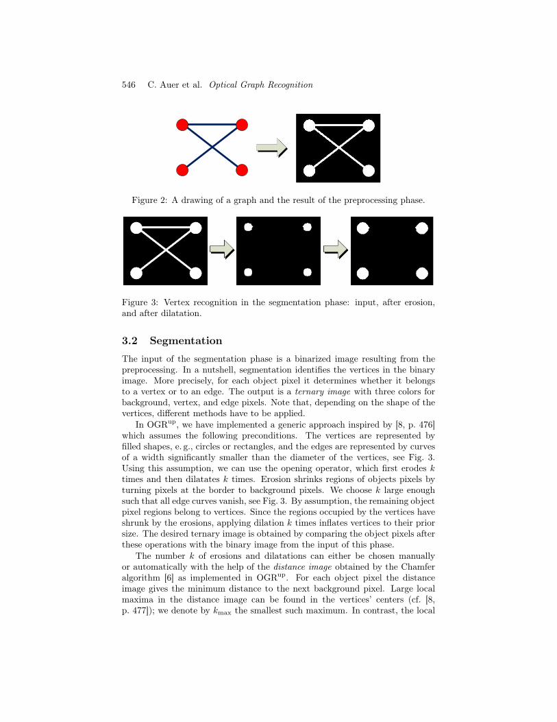
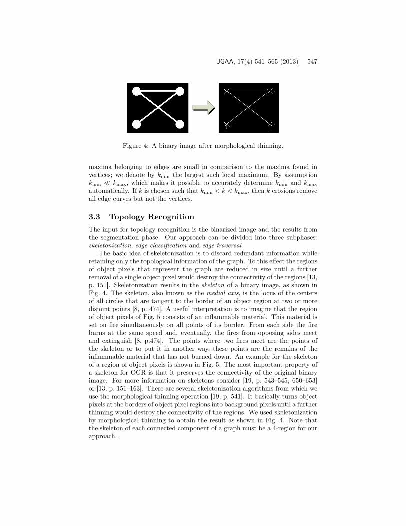
Figure 4: A binary image after morphological thinning.

maxima belonging to edges are small in comparison to the maxima found invertices; we denote by kmin the largest such local maximum. By assumptionkmin � kmax, which makes it possible to accurately determine kmin and kmax

automatically. If k is chosen such that kmin < k < kmax, then k erosions removeall edge curves but not the vertices.

3.3 Topology RecognitionThe input for topology recognition is the binarized image and the results fromthe segmentation phase. Our approach can be divided into three subphases:skeletonization, edge classification and edge traversal.

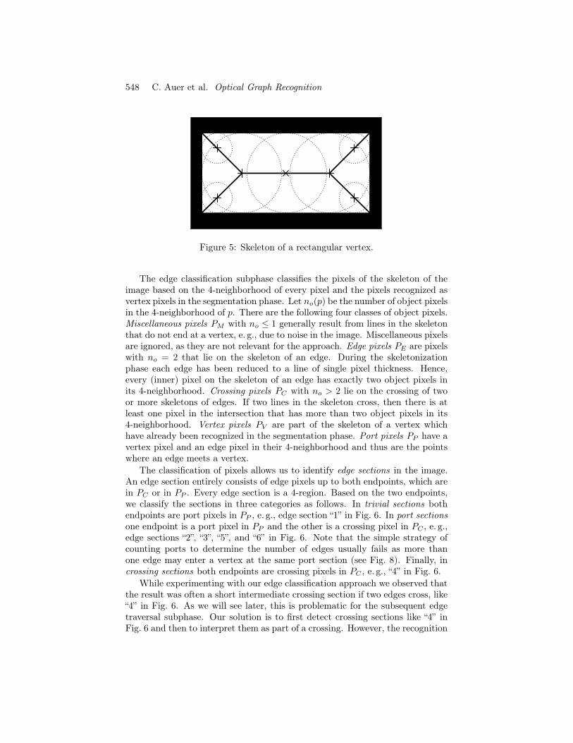
The basic idea of skeletonization is to discard redundant information whileretaining only the topological information of the graph. To this effect the regionsof object pixels that represent the graph are reduced in size until a furtherremoval of a single object pixel would destroy the connectivity of the regions [13,p. 151]. Skeletonization results in the skeleton of a binary image, as shown inFig. 4. The skeleton, also known as the medial axis, is the locus of the centersof all circles that are tangent to the border of an object region at two or moredisjoint points [8, p. 474]. A useful interpretation is to imagine that the regionof object pixels of Fig. 5 consists of an inflammable material. This material isset on fire simultaneously on all points of its border. From each side the fireburns at the same speed and, eventually, the fires from opposing sides meetand extinguish [8, p.474]. The points where two fires meet are the points ofthe skeleton or to put it in another way, these points are the remains of theinflammable material that has not burned down. An example for the skeletonof a region of object pixels is shown in Fig. 5. The most important property ofa skeleton for OGR is that it preserves the connectivity of the original binaryimage. For more information on skeletons consider [19, p. 543–545, 650–653]or [13, p. 151–163]. There are several skeletonization algorithms from which weuse the morphological thinning operation [19, p. 541]. It basically turns objectpixels at the borders of object pixel regions into background pixels until a furtherthinning would destroy the connectivity of the regions. We used skeletonizationby morphological thinning to obtain the result as shown in Fig. 4. Note thatthe skeleton of each connected component of a graph must be a 4-region for ourapproach.

548 C. Auer et al. Optical Graph Recognition

Figure 5: Skeleton of a rectangular vertex.

The edge classification subphase classifies the pixels of the skeleton of theimage based on the 4-neighborhood of every pixel and the pixels recognized asvertex pixels in the segmentation phase. Let no(p) be the number of object pixelsin the 4-neighborhood of p. There are the following four classes of object pixels.Miscellaneous pixels PM with no ≤ 1 generally result from lines in the skeletonthat do not end at a vertex, e. g., due to noise in the image. Miscellaneous pixelsare ignored, as they are not relevant for the approach. Edge pixels PE are pixelswith no = 2 that lie on the skeleton of an edge. During the skeletonizationphase each edge has been reduced to a line of single pixel thickness. Hence,every (inner) pixel on the skeleton of an edge has exactly two object pixels inits 4-neighborhood. Crossing pixels PC with no > 2 lie on the crossing of twoor more skeletons of edges. If two lines in the skeleton cross, then there is atleast one pixel in the intersection that has more than two object pixels in its4-neighborhood. Vertex pixels PV are part of the skeleton of a vertex whichhave already been recognized in the segmentation phase. Port pixels PP have avertex pixel and an edge pixel in their 4-neighborhood and thus are the pointswhere an edge meets a vertex.

The classification of pixels allows us to identify edge sections in the image.An edge section entirely consists of edge pixels up to both endpoints, which arein PC or in PP . Every edge section is a 4-region. Based on the two endpoints,we classify the sections in three categories as follows. In trivial sections bothendpoints are port pixels in PP , e. g., edge section “1” in Fig. 6. In port sectionsone endpoint is a port pixel in PP and the other is a crossing pixel in PC , e. g.,edge sections “2”, “3”, “5”, and “6” in Fig. 6. Note that the simple strategy ofcounting ports to determine the number of edges usually fails as more thanone edge may enter a vertex at the same port section (see Fig. 8). Finally, incrossing sections both endpoints are crossing pixels in PC , e. g., “4” in Fig. 6.

While experimenting with our edge classification approach we observed thatthe result was often a short intermediate crossing section if two edges cross, like“4” in Fig. 6. As we will see later, this is problematic for the subsequent edgetraversal subphase. Our solution is to first detect crossing sections like “4” inFig. 6 and then to interpret them as part of a crossing. However, the recognition

JGAA, 17(4) 541–565 (2013) 549

2

5

3

6

4

1 B

D

A

C

v

Figure 6: A binary image of a graph and the result of edge classification. Anedge pixel is marked with “A”, a vertex pixel with “B”, a port pixel with “C”,and a crossing pixel with “D”. Edge sections are marked with numbers, v andthe small arrows are direction vectors.

of such small crossing sections proved to be difficult. A crossing section mayeither result from a single crossing as “4” in Fig. 6 or may be caused by twoentirely independent crossings as in Fig. 7. In this figure the crossing sections“a”, “b”, “c”, and “d” are interpreted as four adjacent crossing sections and, hence,as a single crossing which is obviously not the case, as seen on the left side ofthe figure. The subsequent edge traversal subphase may recognize the edgeconsisting of sections “1” and “2”, which is not existent in the original drawing.To avoid this problem, our approach is to interpret each crossing section of asize smaller than a predefined parameter as part of a single crossing. Dependingon how thick the edges of a graph are drawn, values for the parameter between5 and 15 pixels lead to suitable results in OGRup [1].

Trivial sections directly connect two vertices without interfering with anyother edges. For every trivial section we directly obtain an edge, e. g., section“1” in Fig. 6. In contrast, port and crossing sections need a more elaboratetreatment as these sections are caused by crossings. In the edge traversal phase,we merge port and crossing sections “adequately” to edges. For example in Fig. 6,sections “2”, “4”, and “6” are merged to one edge as well as “3”, “4”, and “5”. Westart the traversal always at a port section and traverse it until we find a pixelthat is common to two or more edge sections. At this point we determine theadjacent edge section which most probably belongs to the current section usingdirection vectors. The direction vector of an edge section e = (p1, p2, . . . , pl) is atwo dimensional vector −−→pipj with i 6= j, 1 ≤ i, j ≤ l, which defines the directionof e. pi is the tail and pj the head of the vector. Let (xi, yi) be the coordinates

550 C. Auer et al. Optical Graph Recognition

1

c

a

d

b

2

Figure 7: A binary image of a graph and the result of the edge classificationsubphase where every crossing section is interpreted as part of a crossing.

of pi and (xj , yj) the coordinates of pj . Then, −−→pipj = (xj−xi, yj−yi). |i− j|+1is the magnitude of −−→pipj . An example is illustrated in Fig. 6, where we startat port section “2”, reach crossing “D” and then compare the directions of portsection “3” and crossing section “4” with the direction of “2”. In this case “4” ischosen, since its direction is most similar to the direction of “2”. It is importantthat the direction vector of an edge section does not take the whole section intoaccount. That is, the direction vector of “2” is not

−−→CD but computed only from

the immediate area around the crossing. This is primarily necessary for graphswith non-straight edges, where the edges are arbitrary Jordan curves. Hence,when approaching an edge crossing, only the local direction must be used todetermine the most likely subsequent edge section. In our implementation weuse direction vectors with the same magnitude for all edge sections.

During skeletonization it may happen that the directions of edge sections inthe vicinity of a crossing are distorted, which can lead to false results. To avoidthis problem, we do not choose the head of the direction vector directly at thecrossing, but a few pixels away from the crossing when determining directionvectors. For example in Fig. 6, the head of the direction vector of “2” is notpixel “D”.

Continuing with the example from Fig. 6, we may determine an edge consist-ing of “2” followed by “4”. Then both sections “5” and “6” are suitable follow-upsections when only considering the direction vector of “4”. To resolve this, weadditionally take the direction vector of the preceding edge section (if existent)into account as indicated by direction vector “v” in Fig. 6, i. e., v =

−→4 + α · −→2 .

Let ei be the edge section for which the subsequent section must be determined,−→pq the direction vector of ei, and e the current edge of which ei is part of. Ife consists of more than one edge section, we take the predecessor ei−1 of eiin e, determine the direction vector of ei−1 denoted by −→op, and compute thedirection vector of ei as −→pq′ = −→pq + α· −→op with 0 ≤ α ≤ 1. The reason for the αweighting is to reduce the influence of −→op on the final direction vector −→pq′. Therelaxation is to reduce the influence of prior edge sections to avoid unsolicitedresults. Due to this modification, section “6” is chosen as the succeeding section

JGAA, 17(4) 541–565 (2013) 551

A

B

2

1

4

5

3

Figure 8: Binary image of a graph and the result of the edge classificationsubphase. In the lower image (zoomed to the left part of the skeleton) tworecognized crossings “A” and “B” have an odd number of adjacent edge sections.

of “4” and as “6” is a port section, we have recognized an edge of the graphconsisting of “2”, “4”, and “6”. In the same way, the edge consisting of “3”, “4”,and “5” is recognized. With the edge consisting of “1” we now have recognizedthe topology of the input with four vertices and three edges.

Note that the idea to use matching in a straight-forward manner to resolvecrossings yields inferior results to the approach shown in this section. For ex-ample, in Fig. 8 there are crossings with an odd number of adjacent sections.

3.4 Postprocessing

The postprocessing phase concludes OGR and includes procedures that use thetopological structure as input. In OGRup, the postprocessing phase assignscoordinates to the vertices obtained in the segmentation phase. Further, itassigns bends to every edge such that they resemble their counterparts from the

552 C. Auer et al. Optical Graph Recognition

original image. To obtain the coordinates of the bends, each edge is sampledevery i pixels, where i is a user parameter, e. g., i = 10 leads to sufficientlysmooth curves.

4 Experimental ResultsOur prototype OGRup assumes the following preconditions. The vertices aredrawn as filled shapes, e. g., circles or rectangles and all vertices have approx-imately the same size. The edges are represented by curves of a width signifi-cantly smaller than the diameter of the vertices, and they should be contiguousand should exactly end at the vertices.

As a rule of thumb, the easier a graph is be recognized by a human, the betterthe graph is be recognized by OGRup. Our first experiments with OGRup showthat graph recognition is error-prone if many edges cross in a local area and ifedges cross in a small angle. This parallels recent empirical evaluations [20,22],which report that right angle crossings are as legible as no crossings and haveled to the introduction of RAC drawings [15].

Plane drawings of graphs have no crossings and are recognized very well byOGRup. Graphs with few edge crossings, preferably in a large angle, are alsorecognized well and the same holds for RAC drawings. As already stated inSect. 1, the correct topology can only be recognized if the input is unambiguous[24]. Otherwise, even a human must guess the intention of the graph drawer,e. g., Fig. 17. As for most digital image processing approaches, the results ofOGRup heavily depend on the careful adjustment of the necessary parameters.

Experiments with OGRup so far include graphs drawn with pencil and paperas in Figs. 9–12, graphs drawn with an image editing tool as in Figs. 13–15, andgraphs drawn with a graph drawing algorithm, for example with Gravisto [3],as in Fig. 16. The hand-made drawings in Figs. 9 and 10 show that OGRup

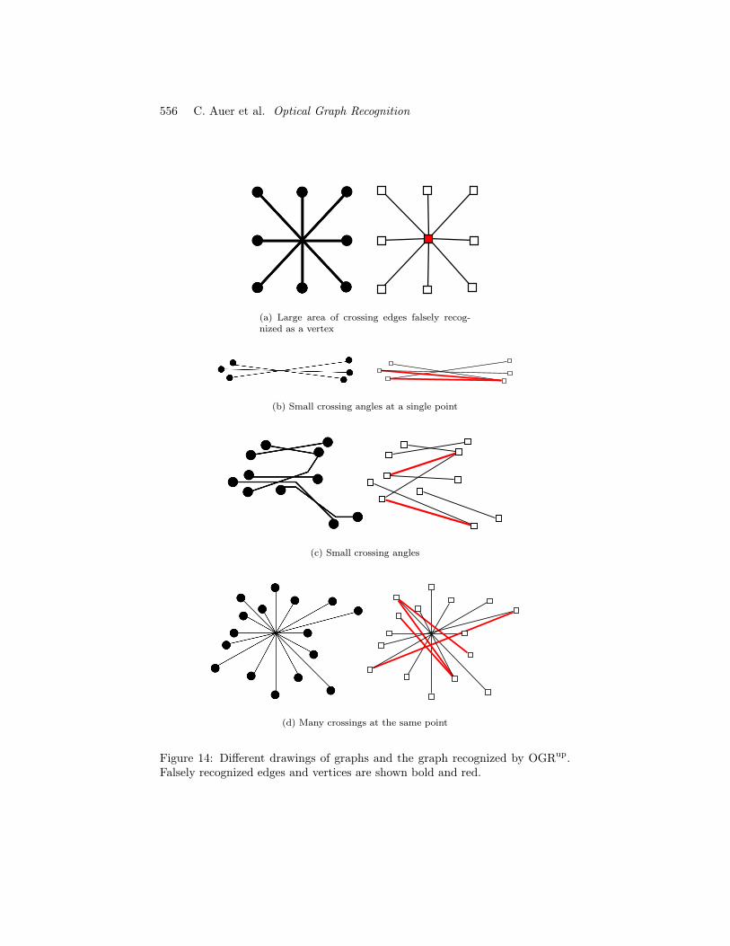
can recognize freehand curves and achieves good results if our preconditions aremet. For the drawing in Fig. 9 a proper adjustment of the parameters in thepreprocessing phase was necessary to ensure that all edges are contiguous andend directly at the vertices. The graphs in Fig. 14 illustrate features of drawingsthat lead to a false recognition by OGRup. In Fig. 14(a) the crossing region hasapproximately the size of a vertex. Hence, OGRup misinterprets the crossing asa vertex. In Figs 14(b-c) the small crossing angles lead to a false recognition.However, all three drawings are also hard to grasp for a human.

As a first benchmark for OGRup, we used the Rome graphs1 (undirectedgraphs with 10 to 100 nodes). Each of the 11534 Rome graphs was drawn 10times in Gravisto [3], with a spring embedder applying the force model fromFruchterman and Reingold [18]. We used a slightly modified Fruchterman andReingold force model, which also models repulsive forces between vertices andtheir non-incident edges to avoid crossings between them. 107543 drawings(93.24%) were correctly recognized. In 50 drawings, large regions of many cross-ing edges were erroneously recognized as vertices.

1http://www.graphdrawing.org/data.html

JGAA, 17(4) 541–565 (2013) 553

Figure 9: A drawing of a 5-dimensional hypercube “Q5” by David Eppstein iscorrectly recognized by OGRup. In the drawing the topmost edge is not con-tiguous and the bottommost edge does not end at a vertex (shown magnified).This problem was resolved by applying opening and closing in the preprocessingphase.

Figure 10: The “T ∗11” graph by Till Bruckdorfer is correctly recognized byOGRup. Multi-edges are shown bold and red.

554 C. Auer et al. Optical Graph Recognition

Figure 11: On the right side a drawing of the Harries-Wong (3,10)-cage from [25,p.272]. The hand drawn graph on the left side has three multi-edges. Withoutthe multi-edges, the two graphs are isomorphic.

Figure 12: The “Double Circulant” graph by Steven Chaplick and the graphrecognized by OGRup. Some falsely recognized edges are shown bold and red.The parts of the drawing that led to the falsely recognized edges are shownmagnified.

JGAA, 17(4) 541–565 (2013) 555

(a) Arbitrary Jordan curves as edges

(b) More engulfed Jordan curves as edges

(c) The Dyck graph. Layout from [26]

(d) The Gray Graph. Layout from [27]

Figure 13: Different drawings of graphs and the graph recognized by OGRup.Each graph was correctly recognized.

556 C. Auer et al. Optical Graph Recognition

(a) Large area of crossing edges falsely recog-nized as a vertex

(b) Small crossing angles at a single point

(c) Small crossing angles

(d) Many crossings at the same point

Figure 14: Different drawings of graphs and the graph recognized by OGRup.Falsely recognized edges and vertices are shown bold and red.

JGAA, 17(4) 541–565 (2013) 557

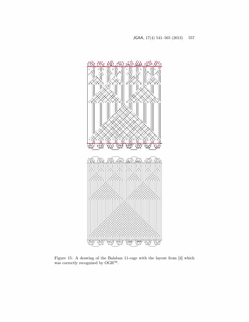
Figure 15: A drawing of the Balaban 11-cage with the layout from [4] whichwas correctly recognized by OGRup.

558 C. Auer et al. Optical Graph Recognition

In the remaining 7747 drawings, the average number of false positives was1.24 (variance 0.51), i. e., non-existent edges of the original graphs were erro-neously recognized by OGRup (cf. Fig. 14(d)). The average number of falsenegatives was 0.14 (variance 0.97), i. e., edges not recognized by OGRup. Themaximum number of false positives and false negatives in a graph was 10 and5, respectively. 77.25% (75.96%) of all false positives (negatives) occurred indrawings with more than 75 vertices. This is caused by many edge crossings insmall areas and small crossing angles, which frequently occur for larger graphs.Altogether, OGRup resulted in 1069 false negatives, i. e., 99.99% of all 7965120edges were recognized and the number of false positives was 9681.

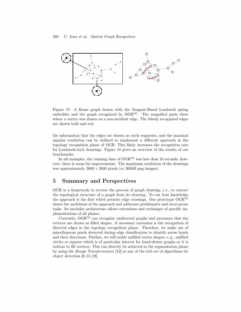
In order to test a different graph drawing algorithm as a benchmark, theRome graphs were drawn with the Lombardi spring embedder from [9]. In aLombardi drawing [16] edges are drawn as circular arcs. It achieves the maxi-mum angular resolution possible at each vertex. We ran separate benchmarkswith the Tangent-Based and the Dummy-Vertex Lombardi spring embedders.The Tangent-Based approach is able to achieve near-perfect angular resolutionat all nodes. However, a problem for OGR is that the algorithm often drawsvertices on top of non-incident edges [9], which are then recognized as beingincident, see Fig. 17. With the additional context information that the graphis a Lombardi-drawing, these falsely recognized edges can possibly be detectedand corrected in the postprocessing phase. For instance, in this case the angularresolution is not (close to) maximal at the vertex. While the Dummy-Vertex ap-proach is less successful in producing near-perfect angular resolution, it increasesthe distances between vertices and non-incident edges [9] and thus reduces theprobability of a vertex being drawn on a non-incident edge.

Every Rome graph was drawn three times with both Lombardi spring em-bedders. With the Tangent-Based approach, OGRup recognized 9502 drawings(37.79%) correctly. In three drawings OGRup failed to recognize the correctnumber of vertices. In the remaining 25097 drawings, the average number offalse positives was 8.60 (variance 47.97) and the average number of false neg-atives was 3.27 (variance 6.62). The maximum number of false positives andfalse negatives in a graph was 58 and 22, respectively. The high number of falsepositives (negatives) results from drawings where vertices are drawn on edges.Here, OGRup resulted in 82066 false negatives, i. e., 96.57% of all 2389536 edgeswere recognized and the number of false positives was 215840.

With the Dummy-Vertex approach, OGRup correctly recognized 13884 draw-ings (40.12%). In 42 drawings OGRup failed to recognize the correct number ofvertices. In the remaining 20676 drawings, the average number of false positiveswas 6.16 (variance 27.50) and the average number of false negatives was 2.18(variance 3.68). The maximum number of false positives and false negatives ina graph was 46 and 18, respectively. In total, OGRup resulted in 45206 falsenegatives, i. e., 98.11% of all 2389536 edges were recognized and the number offalse positives was 127810.

For the Lombardi spring embedders the recognition rate of OGRup is inferioras for the Fruchterman and Reingold spring embedder. However, one might usethe context information that a drawing is in Lombardi-style. For instance,

JGAA, 17(4) 541–565 (2013) 559

(a) A sample Rome graph, which was not correctly recog-nized by OGRup. The part of the drawing that led to afalse recognition is shown magnified.

(b) This Rome graph was correctly recognized byOGRup.

Figure 16: Two drawings of Rome graphs.

560 C. Auer et al. Optical Graph Recognition

Figure 17: A Rome graph drawn with the Tangent-Based Lombardi springembedder and the graph recognized by OGRup. The magnified parts showwhere a vertex was drawn on a non-incident edge. The falsely recognized edgesare shown bold and red.

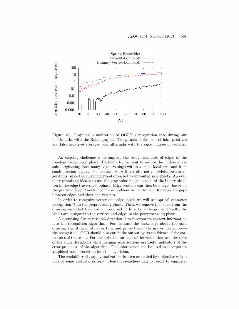
the information that the edges are drawn as circle segments, and the maximalangular resolution can be utilized to implement a different approach in thetopology recognition phase of OGR. This likely increases the recognition ratefor Lombardi-style drawings. Figure 18 gives an overview of the results of ourbenchmarks.

In all examples, the running time of OGRup was less than 10 seconds, how-ever, there is room for improvements. The maximum resolution of the drawingswas approximately 2600× 2600 pixels (or 360kB png images).

5 Summary and PerspectivesOGR is a framework to reverse the process of graph drawing, i. e., to extractthe topological structure of a graph from its drawing. To our best knowledgethe approach is the first which permits edge crossings. Our prototype OGRup

shows the usefulness of the approach and addresses problematic and error-pronetasks. Its modular architecture allows extensions and exchanges of specific im-plementations of all phases.

Currently, OGRup can recognize undirected graphs and presumes that thevertices are drawn as filled shapes. A necessary extension is the recognition ofdirected edges in the topology recognition phase. Therefore, we make use ofmiscellaneous pixels detected during edge classification to identify arrow headsand their directions. Further, we will tackle unfilled vertex shapes, e. g., unfilledcircles or squares which is of particular interest for hand-drawn graphs as it istedious to fill vertices. This can directly be achieved in the segmentation phaseby using the Hough Transformation [12] or any of the rich set of algorithms forobject detection [8, 13,19].

JGAA, 17(4) 541–565 (2013) 561

0.0001

0.001

0.01

0.1

1

10

100

10 20 30 40 50 60 70 80 90 100avg(falsepo

sitives+

negatives)

|V|

Spring-EmbedderTangent-Lombardi

Dummy-Vertex-Lombardi

Figure 18: Graphical visualization of OGRup’s recognition rate during ourbenchmarks with the Rome graphs. The y−axis is the sum of false positivesand false negatives averaged over all graphs with the same number of vertices.

An ongoing challenge is to improve the recognition rate of edges in thetopology recognition phase. Particularly, we want to reduce the undesired re-sults originating from many edge crossings within a small local area and fromsmall crossing angles. For instance, we will test alternative skeletonization al-gorithms, since the current method often led to unwanted side effects. An evenmore promising idea is to use the gray-value image instead of the binary skele-ton in the edge traversal subphase. Edge sections can then be merged based onthe gradient [19]. Another common problem in hand-made drawings are gapsbetween edges and their end vertices.

In order to recognize vertex and edge labels we will use optical characterrecognition [7] in the preprocessing phase. Then, we remove the labels from thedrawing such that they are not confused with parts of the graph. Finally, thelabels are assigned to the vertices and edges in the postprocessing phase.

A promising future research direction is to incorporate context informationinto the recognition algorithm. For instance the knowledge about the useddrawing algorithm or style, or type and properties of the graph may improvethe recognition. OGR should also enrich the output by its confidence of the cor-rectness of the result. For example, the variance of the vertex sizes and the sizesof the angle deviations while merging edge sections are useful indicators of theerror-proneness of the algorithm. This information can be used to incorporategraphical user interaction into the algorithm.

The readability of graph visualizations is often evaluated by subjective weight-ings of some aesthetic criteria. Hence, researchers had to resort to empirical

562 C. Auer et al. Optical Graph Recognition

studies measuring how fast and accurate a human subject group can recognizegraphs. However, the approach is biased due to individual performance andpreferences [21]. Here, OGR may serve as an objective evaluator. The recogni-tion rate of OGRup can be interpreted as a quality indicator. However, thereare some features of drawings which pose no difficulties for OGR but do notmeet common aesthetic criteria. Examples are hard to follow long edges likeintertwined spirals or numerous crossings despite of large crossing angles, e. g.,see Fig. 15.

Last but not least, we are working on a version of OGRup that is compatiblewith smart phones and tablet computers. Then, the user can directly take apicture of a graph with the built-in camera and use OGRup to recognize thegraph for further processing and interaction.

AcknowledgmentsWe would like to thank David Eppstein, Till Bruckdorfer, Steven Chaplick andthe other participants of the 20th International Symposium on Graph Drawingfor providing hand-drawn graphs. We are grateful to Stephen Kobourov, RomanChernobelskiy and Kathryn Cunningham for providing their Tangent-Based andthe Dummy-Vertex Lombardi spring embedder implementations. Also we wouldlike to thank Peter Barth for discussions and useful hints on image processing.

JGAA, 17(4) 541–565 (2013) 563

References[1] C. Auer, C. Bachmaier, F. J. Brandenburg, A. Gleißner, and J. Reislhuber.

Calibration in optical graph recognition. Imagen-A, 3(5), 2013.

[2] C. Auer, C. Bachmaier, F. J. Brandenburg, A. Gleißner, and J. Reisl-huber. Optical graph recognition. In W. Didimo and M. Patriganai,editors, Graph Drawing, LNCS, pages 529–540. Springer, 2013. doi:10.1007/978-3-642-36763-2_47.

[3] C. Bachmaier, F. J. Brandenburg, M. Forster, P. Holleis, and M. Raitner.Gravisto: Graph visualization toolkit. In J. Pach, editor, Graph Drawing,GD 2004, volume 3383 of LNCS, pages 502–503. Springer, 2004. http://gravisto.fim.uni-passau.de/. doi:10.1007/978-3-540-31843-9_52.

[4] Balaban 11-cage alternative drawing, Nov 2012. http://commons.wikimedia.org/w/index.php?title=File:Balaban_11-cage_alternative_drawing.svg&page=1.

[5] S. Birk. Graph recognition from image. Master’s thesis, University ofLjubljana, 2010. http://eprints.fri.uni-lj.si/1250/ (in Slovene).

[6] G. Borgefors. Distance transformations in digital images. Computer Vi-sion, Graphics and Image Processing, 34(3):344–371, 1986. doi:10.1016/S0734-189X(86)80047-0.

[7] H. Bunke and P. S. Wang. Handbook of Character Recognition and Docu-ment Image Analysis. World Scientific, 1997. doi:10.1142/2757.

[8] K. R. Castleman. Digital Image Processing. Prentice-Hall, 1996.

[9] R. Chernobelskiy, K. I. Cunningham, M. T. Goodrich, S. G. Kobourov, andL. Trott. Force-directed Lombardi-style graph drawing. In M. van Kreveldand B. Speckmann, editors, Graph Drawing, GD 2011, volume 7034 ofLNCS, pages 320–331. Springer, 2012. doi:10.1007/978-3-642-25878-7_31.

[10] C. K. Chow and T. Kaneko. Automatic boundary detection of the leftventricle from cineangiograms. Comput. Biomed. Res., 5(4):388–410, 1972.doi:10.1016/0010-4809(72)90070-5.

[11] A.-P. Condurache and T. Aach. Vessel segmentation in angiograms usinghysteresis thresholding. In IAPR Conference on Machine Vision Applica-tions 2005, pages 269–272, 2005.

[12] E. R. Davies. A modified Hough scheme for general circle location. PatternRecogn. Lett., 7(1):37–43, 1988. doi:10.1016/0167-8655(88)90042-6.

[13] E. R. Davies. Machine Vision: Theory, Algorithms, Practicalities. Aca-demic Press, 2nd edition, 1997.

564 C. Auer et al. Optical Graph Recognition

[14] G. Di Battista, P. Eades, R. Tamassia, and I. G. Tollis. Graph Drawing:Algorithms for the Visualization of Graphs. Prentice Hall, 1999.

[15] W. Didimo, P. Eades, and G. Liotta. Drawing graphs with right anglecrossings. Theor. Comput. Sci., 412(39):5156–5166, 2011. doi:10.1016/j.tcs.2011.05.025.

[16] C. A. Duncan, D. Eppstein, M. T. Goodrich, S. G. Kobourov, and M. Nöl-lenburg. Lombardi drawings of graphs. J. Graph Alg. App., 16(2):85–108,2010. doi:10.1007/978-3-642-18469-7_18.

[17] R. Estrada and C. Tomasi. Manuscript bleed-through removal via hysteresisthresholding. In Proc. International Conference on Document Analysisand Recognition, ICDAR 2009, pages 753–757. IEEE, 2009. doi:10.1109/ICDAR.2009.88.

[18] T. M. J. Fruchterman and E. M. Reingold. Graph drawing by force-directedplacement. Software: Practice and Experience, 21(11):1129–1164, 1991.doi:10.1002/spe.4380211102.

[19] R. C. Gonzalez and R. E. Woods. Digital Image Processing. Prentice-Hall,2nd edition, 2002.

[20] W. Huang, P. Eades, and S.-H. Hong. Beyond time and error: A cognitiveapproach to the evaluation of graph drawings. In Proc. Beyond Time andErrors: Novel Evaluation Methods for Information Visualization, BELIV2008, pages 3:1–3:8. ACM, 2008. doi:10.1145/1377966.1377970.

[21] W. Huang, P. Eades, and S.-H. Hong. Measuring effectiveness of graphvisualizations: A cognitive load perspective. Inform. Visual., 8(3):139–152,2009. doi:10.1057/ivs.2009.10.

[22] W. Huang, S.-H. Hong, and P. Eades. Effects of crossing angles. InI. Fujishiro, H. Li, and K.-L. Ma, editors, Proc. IEEE Pacific Visu-alization Symposium, PacificVis 2008, pages 41–46. IEEE, 2008. doi:10.1109/PACIFICVIS.2008.4475457.

[23] V. Lauren and G. Pisinger. Automated analysis of vessel diameters inMR images. Visualization, Imaging, and Image Processing, pages 931–936,2004.

[24] J. Pach. Every graph admits an unambiguous bold drawing. InM. van Krefeld and B. Speckmann, editors, Graph Drawing, GD 2011,volume 7034 of LNCS, pages 332–342. Springer, 2012. doi:10.1007/978-3-642-25878-7_32.

[25] R. C. Read and R. J. Wilson. An Atlas of Graphs. Oxford University Press,1998.

JGAA, 17(4) 541–565 (2013) 565

[26] E. W. Weissstein. Dyck graph, Nov 2012. http://mathworld.wolfram.com/DyckGraph.html.

[27] E. W. Weissstein. Gray graph, Nov 2012. http://mathworld.wolfram.com/GrayGraph.html.