optimal combinaison of cfd modeling and statistical learning for short-term wind power forecasting
TRANSCRIPT

Optimal combination of CFD modeling and statistical
learning for short–term wind power forecasting
Stéphane SANQUER & Jérémie JUBAN- meteodyn
Wind power depends on the volability of the wind
Two times scale are relevant : one for the wind turbine controle (up
to few sec.), one for the integration of power in the grid (minutes to
weeks)
Why a forecast ?
-Optimise the planning of conventional power plants (3-10h)
-Optimise the value of produced electricity in the market (0-48h)
-Schedule the maintenance of the farm and the transmission lines
(day to week)

The model can be physical, statistical or twice
Very short term statistical approaches use scada as input (look ahead time <6h)
A forecast system for horizons >6h always includes a Numerical Weather Prediction system (NWP) and sometimes a Model Output Statistic system to optimize the forecast (MOS)
•Source : Anemos Project ” The State-Of-The-Art in
Short-Term Prediction of Wind Power”

Average NMAE for 12 hours forecast horizon vs RIX Source: Best Practice in Short-Term Forecasting. A Users Guide
Gregor Giebel(Risø National Laboratory, DTU), George Kariniotakis( Ecole des Mines de Paris)
12 models tested on various terrains to consider the local effects
Errors increase with the terrain complexity.
Terrain modeling can be introduced to improve the
performance of the forecast system.

To define an optimal combination of both physical and statistical
modeling in order to reach the highest forecast performance
To use a learning model (« black box ») based on a data set of
couples measurement/prediction. Here we use a Artificial Neural
Network (ANN)
To minimize the prediction error by introducing automatic
error corrections while keeping the advantage
of the full physical modeling


Global model
0.125 or 0.5 degrees
Resolution
GFS, ECM WF
Mesoscale model .
1 km to 15 km
resolution
WRF.
Microscale
model
25 m resolution
Meteodyn WT
Statistical
modelling
DATA
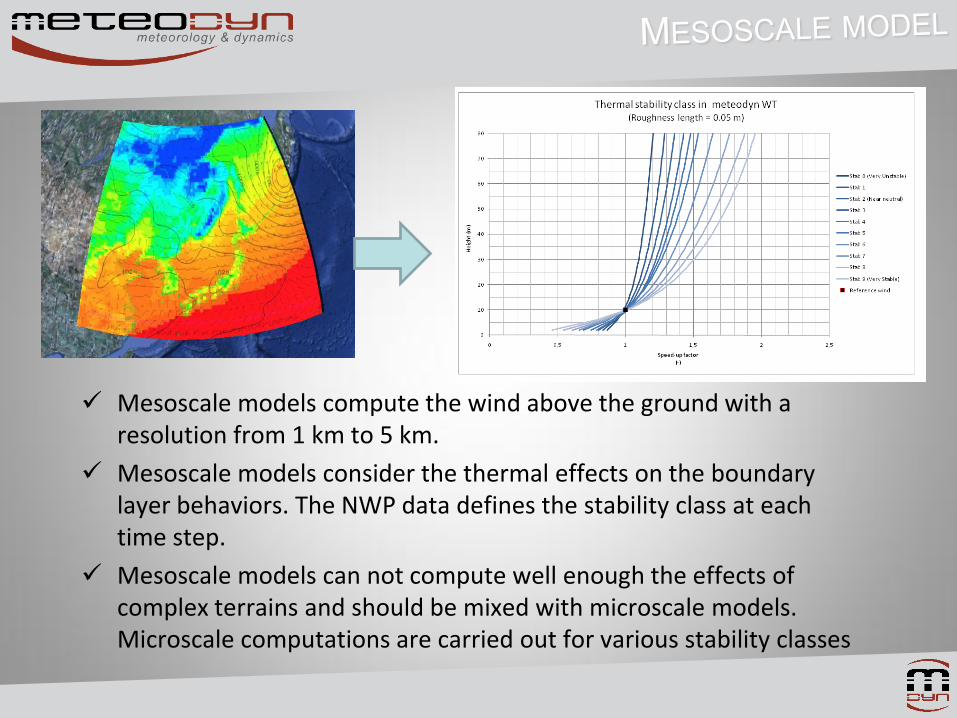
Mesoscale models compute the wind above the ground with a resolution from 1 km to 5 km.
Mesoscale models consider the thermal effects on the boundary layer behaviors. The NWP data defines the stability class at each time step.
Mesoscale models can not compute well enough the effects of complex terrains and should be mixed with microscale models. Microscale computations are carried out for various stability classes

The mesoscale points are transfered to each wind turbine thanks to the « speed coefficients » obtained by the CFD model
Local effects taken into account : Orography, Land-use
The windspeed coefficients allow the statistical correction of NWP data and power curves correction, by using met mast measurements.
Calibration takes into account seasonal variations (snow, foliage density, …)

Global model
0.125 or 0.5 degrees
Resolution
GFS, ECM WF
Mesoscale model .
1 km to 15 km
resolution
WRF.
Microscale
model
25 m resolution
Meteodyn WT
Statistical
modelling
DATA

Global model
0.125 or 0.5 degrees
Resolution
GFS, ECM WF
Mesoscale model .
1 km to 15 km
resolution
WRF.
Microscale
model
25 m resolution
Meteodyn WT
Statistical
modelling
DATA

How to define Neural Network Architecture?
(number of layers, number of neurons)
Increasing complexity
Map several inputs to an output
Input: Forecast power, NWP variables and
production data
Output: wind power or wind speed
The supervised mapping function is learnt from data

Define three sets
A Testing set choose architecture (testing error)
A Training set training the network (training error)
Finally, a validation set computes true error.
Training Error
Testing error
Expected minimum error

Wind Farm in China with a complex terrain and weather regimes
Learning period : 06/2010 to 02/2012
Testing period : 03/2012 to 11/2012
Forecast horizons : +6h to 46h
Forecast steps : 15 min. Runs :4/day
Input variables
NWP : V, Dir, S, T, r,Patm
Park production

Mesoscale modeling is used to compute the wind
above the site
Model GFS/WRF
Resolution 5 km
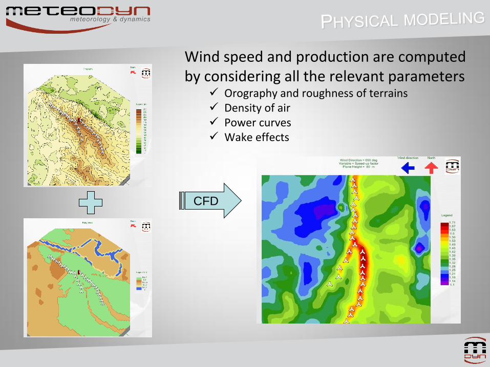
Wind speed and production are computed by considering all the relevant parameters
Orography and roughness of terrains Density of air Power curves Wake effects
CFD

After learning of the ANN model, the production is forecast
and compared to the real production
Production is globally well forecasted
Some time lags are observed

ANN model reduce forecasting errors of pure physical approach
Improvements on MAE and RMSE are respectively 5% and 16%
RMSE reduced to
16% bound
MAE reduced to
10.5% bound
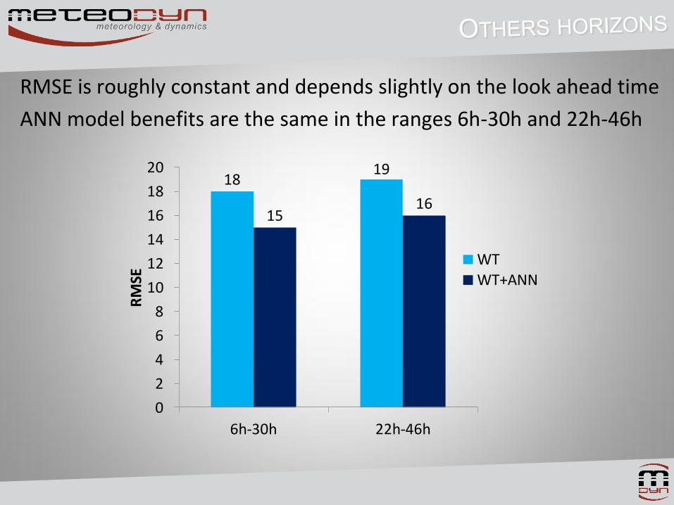
RMSE is roughly constant and depends slightly on the look ahead time
ANN model benefits are the same in the ranges 6h-30h and 22h-46h
18
19
1516
0
2
4
6
8
10
12
14
16
18
20
6h-30h 22h-46h
RM
SE
WT
WT+ANN

An optimal combination of statistical and physical modeling
is central to high performance forecasting
Even for complex terrains, as soon as micro-CFD modeling
is performed, Even with weather regime, by coupling NWP
with Statistical learning for short term wind power forecasting,
RMSE about 15% can be achieved for horizons in the range
6h-48h. MAE reach 10% bound as for flat terrains.
Introducing advanced statistical learning leads to significant
improvement over a pure (even advanced) physical approach