HAL Id: tel-01419791https://hal.archives-ouvertes.fr/tel-01419791

Submitted on 19 Dec 2016

HAL is a multi-disciplinary open accessarchive for the deposit and dissemination of sci-entific research documents, whether they are pub-lished or not. The documents may come fromteaching and research institutions in France orabroad, or from public or private research centers.

L’archive ouverte pluridisciplinaire HAL, estdestinée au dépôt et à la diffusion de documentsscientifiques de niveau recherche, publiés ou non,émanant des établissements d’enseignement et derecherche français ou étrangers, des laboratoirespublics ou privés.

Public Domain

Optimal control problems for the bioremediation ofwater resources

Victor Riquelme

To cite this version:Victor Riquelme. Optimal control problems for the bioremediation of water resources. Optimizationand Control [math.OC]. Université de Montpellier 2; Universidad de Chile, 2016. English. <tel-01419791>

Délivré par l’UNIVERSITÉ DE MONTPELLIERen cotutelle avec l’UNIVERSIDAD DE CHILE

Préparée au sein de l’école doctorale I2SEt de l’unité de recherche UMR MISTEA

Spécialité: Mathématiques et modélisation

Présentée par Víctor RIQUELMEvriquelme@dim.uchile.cl

Optimal control problems forthe bioremediation of water

resources

Soutenue le 20 Septembre 2016 devant le jury composé de

Alain Rapaport Directeur de Recherche, INRA Montpellier DirecteurHéctor Ramírez Professeur, Universidad de Chile CodirecteurTomás Caraballo Professeur, Universidad de Sevilla RapporteurPatrick De Leenheer Professeur, Oregon State University RapporteurAlejandro Jofré Professeur, Universidad de Chile (President du jury) ExaminateurAntoine Rousseau Chargé de recherche, Université de Montpellier ExaminateurFrancisco Silva Maître de conférences, Université de Limoges Examinateur

ii

RÉSUMÉ

Cette thèse se compose de deux parties. Dans la première partie, nous étudions les stratégies de tempsminimum pour le traitement de la pollution dans de grandes ressources en eau, par exemple des lacsou réservoirs naturels, à l’aide d’un bioréacteur continu qui fonctionne à un état quasi stationnaire. Oncontrôle le débit d’entrée d’eau au bioréacteur, dont la sortie revient à la ressource avec le même débit.Nous disposons de l’hypothèse d’homogénéité de la concentration de polluant dans la ressource en pro-posant trois modèles spatialement structurés. Le premier modèle considère deux zones connectées l’uneà l’autre par diffusion et seulement une d’entre elles connectée au bioréacteur. Avec l’aide du Principedu Maximum de Pontryagin, nous montrons que le contrôle optimal en boucle fermée dépend seulementdes mesures de pollution dans la zone traitée, sans influence des paramètres de volume, diffusion, oula concentration dans la zone non traitée. Nous montrons que l’effet d’une pompe de recirculation quiaide à homogénéiser les deux zones est avantageux si opérée à vitesse maximale. Nous prouvons quela famille de fonctions de temps minimal en fonction du paramètre de diffusion est décroissante. Ledeuxième modèle consiste en deux zones connectées l’une à l’autre par diffusion et les deux connec-tées au bioréacteur. Ceci est un problème dont l’ensemble des vitesses est non convexe, pour lequel iln’est pas possible de prouver directement l’existence des solutions. Nous surmontons cette difficulté etrésolvons entièrement le problème étudié en appliquant le principe de Pontryagin au problème de con-trôle relaxé associé, obtenant un contrôle en boucle fermée qui traite la zone la plus polluée jusqu’aul’homogénéisation des deux concentrations. Nous obtenons des limites explicites sur la fonction valeurvia des techniques de Hamilton-Jacobi-Bellman. Nous prouvons que la fonction de temps minimal estnon monotone par rapport au paramètre de diffusion. Le troisième modèle consiste en deux zones con-nectées au bioréacteur en série et une pompe de recirculation entre elles. L’ensemble des contrôlesdépend de l’état, et nous montrons que la contrainte est active à partir d’un temps jusqu’à la fin duprocessus. Nous montrons que le contrôle optimal consiste à l’atteinte d’un temps à partir duquel il estoptimal de recirculer à vitesse maximale et ensuite ré-polluer la deuxième zone avec la concentrationde la première. Ce résultat est non intuitif. Les stratégies optimales obtenues sont testées sur des mod-èles hydrodynamiques, en montrant qu’elles sont de bonnes approximations de la solution du problèmeinhomogène. La deuxième partie consiste au développement et l’étude d’un modèle stochastique deréacteur biologique séquentiel. Le modèle est obtenu comme une limite des processus de naissance etde mort. Nous établissons l’existence et l’unicité des solutions de l’équation contrôlée qui ne satisfaitpas les hypothèses habituelles. Nous prouvons que pour n’importe quelle loi de contrôle la probabilitéd’extinction de la biomasse est positive. Nous étudions le problème de la maximisation de la probabil-ité d’atteindre un niveau de pollution cible, avec le réacteur à sa capacité maximale, avant l’extinction.Ce problème ne satisfait aucune des suppositions habituelles, donc le problème doit être étudié dansdeux étapes: en premier lieu, nous prouvons la continuité de la fonction de coût non contrôlée pour lesconditions initiales avec le volume maximal et ensuite nous développons un principe de programmationdynamique pour une modification du problème original comme un problème de contrôle optimal aveccoût final sans contrainte sur l’état.

Mots clés: Contrôle optimal, temps minimal, contrôle stochastique, biorestauration, chemostat.

iii

iv

ABSTRACT

This thesis consists of two parts. In the first part we study minimal time strategies for the treatment ofpollution in large water volumes, such as lakes or natural reservoirs, using a single continuous bioreactorthat operates in a quasi-steady state. The control consists of feeding the bioreactor from the resource,with clean output returning to the resource with the same flow rate. We drop the hypothesis of ho-mogeneity of the pollutant concentration in the water resource by proposing three spatially structuredmodels. The first model considers two zones connected to each other by diffusion and only one of themtreated by the bioreactor. With the help of the Pontryagin Maximum Principle, we show that the optimalstate feedback depends only on the measurements of pollution in the treated zone, with no influence ofvolume, diffusion parameter, or pollutant concentration in the untreated zone. We show that the effectof a recirculation pump that helps to mix the two zones is beneficial if operated at full speed. We provethat the family of minimal time functions depending on the diffusion parameter is decreasing. The sec-ond model consists of two zones connected to each other by diffusion and each of them connected tothe bioreactor. This is a problem with a non convex velocity set for which it is not possible to directlyprove the existence of its solutions. We overcome this difficulty and fully solve the studied problemapplying Pontryagin’s principle to the associated problem with relaxed controls, obtaining a feedbackcontrol that treats the most polluted zone up to the homogenization of the two concentrations. We alsoobtain explicit bounds on its value function via Hamilton-Jacobi-Bellman techniques. We prove that theminimal time function is nonmonotone as a function of the diffusion parameter. The third model consistsof a system of two zones connected to the bioreactor in series, and a recirculation pump between them.The control set depends on the state variable; we show that this constraint is active from some time upto the final time. We show that the optimal control consists of waiting up to a time from which it isoptimal the mixing at maximum speed, and then to repollute the second zone with the concentration ofthe first zone. This is a non intuitive result. Numerical simulations illustrate the theoretical results, andthe obtained optimal strategies are tested in hydrodynamic models, showing to be good approximationsof the solution of the inhomogeneous problem. The second part consists of the development and studyof a stochastic model of sequencing batch reactor. We obtain the model as a limit of birth and deathprocesses. We establish the existence and uniqueness of solutions of the controlled equation that doesnot satisfy the usual assumptions. We prove that with any control law the probability of extinction ispositive, which is a non classical result. We study the problem of the maximization of the probability ofattaining a target pollution level, with the reactor at maximum capacity, prior to extinction. This prob-lem does not satisfy any of the usual assumptions (non Lipschitz dynamics, degenerate locally Hölderdiffusion parameter, restricted state space, intersecting reach and avoid sets), so the problem must bestudied in two stages: first, we prove the continuity of the uncontrolled cost function for initial condi-tions with maximum volume, and then we develop a dynamic programming principle for a modificationof the problem as an optimal control problem with final cost and without state constraint.

Keywords: Optimal control, minimum time, stochastic control, bioremediation, chemostat.

v

vi

RESUMEN

La tesis de compone de dos partes. En la primera parte estudiamos estrategias de tiempo mínimo para eltratamiento de la contaminación en recursos acuíferos de gran volumen, tales como lagos o reservas nat-urales, mediante el uso de un biorreactor continuo que opera en un estado cuasi-estacionario. El controlconsiste en la alimentación del biorreactor desde el recurso, con un efluente más limpio siendo devueltoal recurso con el mismo caudal. Eliminamos la hipótesis de homogeneidad en la concentración delcontaminante en el recurso proponiendo tres modelos espacialmente estructurados. El primer modeloconsidera dos zonas conectadas entre ellas mediante difusión y donde sólo una de ellas es tratada por elbiorreactor. Con la ayuda el Principio del Máximo de Pontryagin probamos que el control retroalimen-tado óptimo depende sólo de las mediciones del contaminante en la zona tratada, sin dependencia delvolumen, de la difusión, o de la concentración del contaminante en la zona no tratada. Mostramos queel efecto de añadir una bomba de recirculación que ayuda a mezclar ambas zonas es benéfico si ésta seopera a su máxima velocidad. El segundo modelo consiste en dos zonas conectadas entre sí por difusióny cada una de ellas conectada al biorreactor. Este es un problema donde el conjunto de velocidades esno convexo y para el cual no es posible probar directamente la existencia de soluciones. Superamosesta dificultad y resolvemos completamente el problema estudiad aplicando el principio de Pontryaginal problema asociado con controles relajados, obteniendo un control retroalimentado que trata le zonamás contaminada hasta la homogeneización de ambas zonas. También obtenemos cotas explícitas sobrela función valor mediante técnicas de Hamilton-Jacobi-Bellman. Probamos que la función de tiempomínimo es no-monótona como función del parámetro de difusión. El tercer modelo consiste en unsistema de dos zonas conectadas al biorreactor en serie, y una bomba de recirculación entre ellas. Elconjunto de controles depende de la variable de estado; mostramos que esta restricción es activa a partirde cierto instante de tiempo hasta el final del proceso. Este es un resultado no intuitivo. Simulacionesnuméricas ilustran los resultados teóricos, y las estrategias obtenidas son testeadas en modelos hidrod-inámicos, mostrando ser buenas aproximaciones de la solución del problema no homogéneo. La segundaparte consiste en el desarrollo y estudio de un modelo estocástico de biorreactor secuencial por lotes.Obtenemos el modelo como un límite de procesos de nacimiento y muerte. Establecemos la existenciay unicidad de soluciones de la ecuación controlada que no satisface las hipótesis usuales. Probamosque para cualquier control, la probabilidad de extinción es positiva, resultado que no es clásico. Estudi-amos el problema de la maximización de la probabilidad de llegar al nivel deseado de contaminación,con el reactor lleno, antes de la extinción. Este problema no satisface ninguna de las hipótesis usuales(dinámica no Lipschitz, coeficiente de difusión degenerado localmente Hölder, restricciones de espaciode estado, conjuntos objetivo y absorbente se intersectan), por lo que el problema debe ser estudiadoen dos etapas: primero, probamos la continuidad de la función de costo sin control para condicionesiniciales con volumen máximo, y luego desarrollamos un principio de programación dinámica para unamodificación del problema como un problema de control óptimo con costo final y sin restricciones deestado.

Palabras claves: Control óptimo, tiempo mínimo, control estocástico, bioremediacion, quimiostato.

vii

viii

L’apprentissage ne se termine jamais.

ix

x

Remerciements

Je voudrais commencer par remercier mes directeurs de thèse Dr. Alain Rapaport (Universitéde Montpellier) et Dr. Héctor Ramírez (Université du Chili) pour leur soutien et leur directionle long de cette thèse; leur appui a été très important au cours de mes études et ma thèse. Jeremercie aussi les professeurs Tomás Caraballo, Patrick De Leenheer, et Francisco Silva d’avoiraccepté aimablement d’être rapporteurs de cette thèse, et aux professeurs Alejandro Jofré etAntoine Rousseau d’avoir accepté de faire partie du jury. Aux professeurs Pedro Gajardo,Joseph Frédéric Bonnans, Térence Bayen, et Jérôme Harmand pour les discussions et leursbonnes idées. Une reconnaissance spéciale au professeur Joaquín Fontbona, pour ses brillantesidées dans la section de modélisation stochastique.

Je remercie le Département d’Ingénierie Mathématique de l’Université du Chili, l’institutiondans laquelle je me suis formé comme ingénieur et dans laquelle j’ai suivi mes études de doc-torat; à ses professeurs et ses fonctionnaires, particulièrement à Silvia Mariano, sans son aideil aurait été difficile d’avancer. Je remercie au Département de Mathématiques de l’Universitéde Montpellier et en particulier à Mme. Bernadette Lacan pour son assistance qui a été trèsimportante pour bien développer la thèse en cotutelle avec l’Université de Montpellier.

Je remercie CONICYT d’avoir financer mes études de doctorat grâce à la bourse BecaDoctorado Nacional Convocatoria 2013 folio 21130840. Cette thèse a été développée dansle contexte des équipes associés DYMECOS INRIA et DYMECOS 2 INRIA, le projet BION-ATURE de CIRIC INRIA CHILE, et elle a été partiellement financé par les projets CONICYTREDES 130067 et MOMARE SticAmsud. Aussi, je remercie le soutien financier de CON-ICYT sous le projet ACT 10336, les projets FONDECYT 1080173, 1110888, 1160204, leprojet BASAL du Centro de Modelamiento Matemático de l’Université du Chili, et le projetMathAmsud N15MATH-02. Je remercie le soutien financier du Départemento de Postgradoy Postítulo de la Vicerrectoría de Asuntos Académicos de l’Université du Chili et l’InstitutFrançais (l’Ambassade de la France au Chili).

Je remercie ma famille par son appui le long de ma vie et de mes études, et ma fiancéePascale, qui m’a appuyée tout ce temps, même dans mes longs séjours à l’étranger sans sacompagnie.

xi

xii

Contents

1 Introduction 11.1 Bioprocesses and bioremediation . . . . . . . . . . . . . . . . . . . . . . . . . 11.2 Mathematical models of bioreactors and classical results . . . . . . . . . . . . 4

1.2.1 Mathematical models . . . . . . . . . . . . . . . . . . . . . . . . . . . 41.2.2 Classical results on chemostats . . . . . . . . . . . . . . . . . . . . . . 71.2.3 Classical results on SBRs . . . . . . . . . . . . . . . . . . . . . . . . 111.2.4 Stochastic models of bioreactors . . . . . . . . . . . . . . . . . . . . . 13

1.3 Model of inhomogeneous lake . . . . . . . . . . . . . . . . . . . . . . . . . . 151.4 Singular perturbations . . . . . . . . . . . . . . . . . . . . . . . . . . . . . . . 191.5 Contributions of the thesis . . . . . . . . . . . . . . . . . . . . . . . . . . . . 22

1.5.1 Deterministic optimal control for continuous bioremediation processes 221.5.2 Study of stochastic modeling of sequencing batch reactors . . . . . . . 27

2 Bioremediation of natural water resourcesvia Optimal Control techniques 292.1 Introduction . . . . . . . . . . . . . . . . . . . . . . . . . . . . . . . . . . . . 292.2 Mathematical model . . . . . . . . . . . . . . . . . . . . . . . . . . . . . . . 31

2.2.1 Description of the dynamics . . . . . . . . . . . . . . . . . . . . . . . 312.2.2 Preliminary results on the dynamics . . . . . . . . . . . . . . . . . . . 332.2.3 Minimal time optimal control problem . . . . . . . . . . . . . . . . . . 34

2.3 Application of Pontryagin maximum principle . . . . . . . . . . . . . . . . . 352.4 The effect of recirculation . . . . . . . . . . . . . . . . . . . . . . . . . . . . . 372.5 Numerical Simulations . . . . . . . . . . . . . . . . . . . . . . . . . . . . . . 402.6 Conclusion . . . . . . . . . . . . . . . . . . . . . . . . . . . . . . . . . . . . 41

3 Optimal feedback synthesis and minimal time function for the bioremediation ofwater resources with two patches 433.1 Introduction . . . . . . . . . . . . . . . . . . . . . . . . . . . . . . . . . . . . 433.2 Definitions and preliminaries . . . . . . . . . . . . . . . . . . . . . . . . . . . 453.3 Study of the relaxed problem . . . . . . . . . . . . . . . . . . . . . . . . . . . 493.4 Synthesis of the optimal strategy . . . . . . . . . . . . . . . . . . . . . . . . . 543.5 Study of the minimal-time function . . . . . . . . . . . . . . . . . . . . . . . . 553.6 Numerical illustrations . . . . . . . . . . . . . . . . . . . . . . . . . . . . . . 613.7 Conclusion . . . . . . . . . . . . . . . . . . . . . . . . . . . . . . . . . . . . 64

4 Minimal-time bioremediation of natural water resources with gradient of pollu-

xiii

tant 674.1 Introduction . . . . . . . . . . . . . . . . . . . . . . . . . . . . . . . . . . . . 674.2 Definitions and preliminaries . . . . . . . . . . . . . . . . . . . . . . . . . . . 694.3 Optimal control problem . . . . . . . . . . . . . . . . . . . . . . . . . . . . . 704.4 Numerical simulations . . . . . . . . . . . . . . . . . . . . . . . . . . . . . . 774.5 Conclusions . . . . . . . . . . . . . . . . . . . . . . . . . . . . . . . . . . . . 79

5 Stochastic modelling of sequencing batch reactors for wastewater treatment 805.1 Introduction . . . . . . . . . . . . . . . . . . . . . . . . . . . . . . . . . . . . 805.2 Stochastic SBR model . . . . . . . . . . . . . . . . . . . . . . . . . . . . . . 815.3 Existence of solutions of the controlled stochastic model . . . . . . . . . . . . 895.4 The optimal reach-avoid problem . . . . . . . . . . . . . . . . . . . . . . . . . 955.5 Numerical simulations and conclusions . . . . . . . . . . . . . . . . . . . . . 101

6 Conclusions and perspectives 104

Bibliography 109

xiv

List of Tables

2.1 Comparison between optimal treatment time and the time given by the bestconstant control, from initial condition z = (5, 8) . . . . . . . . . . . . . . . . 40

2.2 Comparison between optimal treatment time and the time given by the bestconstant control, from initial condition z = (6, 7) . . . . . . . . . . . . . . . . 40

2.3 Comparison between optimal treatment time and the time given by the bestconstant control, from initial condition z = (2, 10) . . . . . . . . . . . . . . . 40

2.4 Comparison of optimal times with respect to diffusion parameterD from initialcondition z = (5, 8) . . . . . . . . . . . . . . . . . . . . . . . . . . . . . . . . 41

2.5 Comparison of optimal times with respect to diffusion parameterD from initialcondition z = (6, 7) . . . . . . . . . . . . . . . . . . . . . . . . . . . . . . . . 41

2.6 Comparison of optimal times with respect to diffusion parameterD from initialcondition z = (2, 10) . . . . . . . . . . . . . . . . . . . . . . . . . . . . . . . 41

3.1 Time comparisons (in hours) for r = 0.3 and target value s = 1 (top), 0.1(bottom) [g/l] (initial condition s(0) and diffusion parameter d are given in [g/l]and [1/h], respectively) . . . . . . . . . . . . . . . . . . . . . . . . . . . . . . 63

4.1 Comparison of treatment times for the optimal strategies . . . . . . . . . . . . 774.2 Comparison of optimal times with respect to maximum recirculation parameter

QR for different initial conditions . . . . . . . . . . . . . . . . . . . . . . . . . 77

xv

List of Figures

1.1 Scheme of water treatment . . . . . . . . . . . . . . . . . . . . . . . . . . . . 31.2 Industrial bioreactor . . . . . . . . . . . . . . . . . . . . . . . . . . . . . . . . 31.3 Scheme bioreactor-settler . . . . . . . . . . . . . . . . . . . . . . . . . . . . . 31.4 Typical growth functions. On the left, the Monod uptake function; on the right,

the Haldane uptake function. . . . . . . . . . . . . . . . . . . . . . . . . . . . 61.5 Trajectories on the phase portrait, depending on the diffusion parameter D. In

green, the washout equilibrium; in red, the nontrivial equilibrium. . . . . . . . 81.6 Equilibrium points for the Monod growth function. We see that D1 < µmax,

and then the concentration of substrate at equilibrium is s†r = λ1. For D2, theequilibrium is the washout. . . . . . . . . . . . . . . . . . . . . . . . . . . . . 9

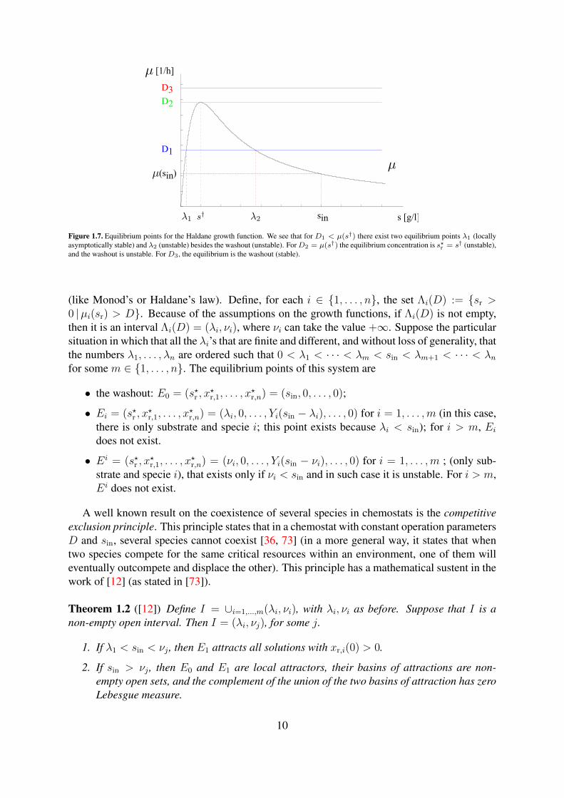
1.7 Equilibrium points for the Haldane growth function. We see that for D1 <µ(s†) there exist two equilibrium points λ1 (locally asymptotically stable) andλ2 (unstable) besides the washout (unstable). For D2 = µ(s†) the equilibriumconcentration is s?r = s† (unstable), and the washout is unstable. For D3, theequilibrium is the washout (stable). . . . . . . . . . . . . . . . . . . . . . . . . 10

1.8 Relation between fictitious time τ and real time t . . . . . . . . . . . . . . . . 131.9 Behavior of the inhomogeneous representation of a lake. From the homoge-

neous initial distribution of pollutant (on the left), the system evolves up to apoint in which two zones are clearly differentiated (on the right). Taken from [4] 17

1.10 First model of inhomogeneity: the active-dead zones configuration . . . . . . . 181.11 Second model of inhomogeneity: the model with two patches . . . . . . . . . . 181.12 Third model of inhomogeneity: the configuration in series with recirculation . . 191.13 Total pollutant concentration in the resource of the full dynamics (3.6) with the

strategy (3.25), for different values of ε. . . . . . . . . . . . . . . . . . . . . . 221.14 Velocity set of the dynamic (1.30) when s1 6= s2 . . . . . . . . . . . . . . . . . 25

2.1 Connections between active zone, dead zone and bioreactor. . . . . . . . . . . 302.2 Connections between active zone, dead zone and bioreactor, with the recircu-

lation pumps. . . . . . . . . . . . . . . . . . . . . . . . . . . . . . . . . . . . 37

3.1 Modeling scheme of the treatment of two interconnected patches (definitionsof the variables and parameters are given in Section 3.2) . . . . . . . . . . . . 44

3.2 Graphs of µ(·) and corresponding γ(·). . . . . . . . . . . . . . . . . . . . . . . 613.3 Optimal paths for d = 0.1[h−1] (left) and d = 10[h−1] (right) with r = 0.3. . . . 613.4 Level sets (in hours) of V0 (left) and V∞ (right) for r = 0.3. . . . . . . . . . . . 62

xvi

3.5 Trajectories and controls generated by the two-pumps and one-pump optimalfeedback, for r=0.3, s=1 [g/l] and s(0)=(3,10) [g/l]. On the left d=0.1[1/h], andon the right d=10[1/h]. . . . . . . . . . . . . . . . . . . . . . . . . . . . . . . 64

3.6 Total pollutant concentration in the resource of the full dynamics (3.6) with thestrategy (3.25), for different values of ε. . . . . . . . . . . . . . . . . . . . . . 64

4.1 Modeling scheme of the nonhomogeneity of concentrations in the resource astwo zones, and a recirculation pump. . . . . . . . . . . . . . . . . . . . . . . . 68

4.2 Backward integration of the extremals, with QR = 0. . . . . . . . . . . . . . . 784.3 Backward integration of the extremals, with QR = 1. . . . . . . . . . . . . . . 784.4 Backward integration of the extremals, with QR = 10. . . . . . . . . . . . . . 79

5.1 Plot of the function v for γ = 1 . . . . . . . . . . . . . . . . . . . . . . . . . . 1015.2 Plot of the function v for γ = 5 . . . . . . . . . . . . . . . . . . . . . . . . . . 1025.3 Plot of the function v for γ = 10 . . . . . . . . . . . . . . . . . . . . . . . . . 102

6.1 First extension: model with three patches and two pumps . . . . . . . . . . . . 1066.2 Second extension: problem with two pollutants . . . . . . . . . . . . . . . . . 107

xvii

xviii

Chapter 1

Introduction

1.1 Bioprocesses and bioremediation

Bioremediation is the process that uses living organisms (usually microorganisms) or micro-bial processes to produce molecular transformations or degradations on environmental contam-inants (hazardous to soils, groundwater, sediments, surface water, or air) into products of lesstoxic form. When these changes occur naturally without human intervention, the process iscalled natural attenuation. Nevertheless, the speed of such changes is slow. By means of ap-propriate control techniques these biological systems can be used to enhance the speed of thechanges or degradations, as well as to use them in places with high pollutant concentrations.

Microorganisms have the ability to biodegrade most of the organic contaminants and manyinorganic contaminats, for instance, hydrocarbon, pesticides, herbicides, petroleum, gasoil,heavy metals among others. Biological treatments of organic contaminations are based onthe degradative abilities of the microorganisms [61].

Bioremediation technologies can be broadly classified as ex situ and in situ [8]. Ex situtechnologies are those treatments which involve the physical removal of the contaminated ma-terial for treatment process. In situ techniques involve treatment of the contaminated materialin place. Examples of in situ and ex situ bioremediation are

• Land farming: Solid-phase treatment system for contaminated soils: may be done in situor ex situ.

• Composting: Aerobic, thermophilic treatment process in which contaminated material ismixed with a bulking agent; can be done using static piles or aerated piles.

• Bioreactors: Biodegradation in a container or reactor; may be used to treat liquids orslurries.

• Bioventing: Method of treating contaminated soils by drawing oxygen through the soilto stimulate microbial activity.

1

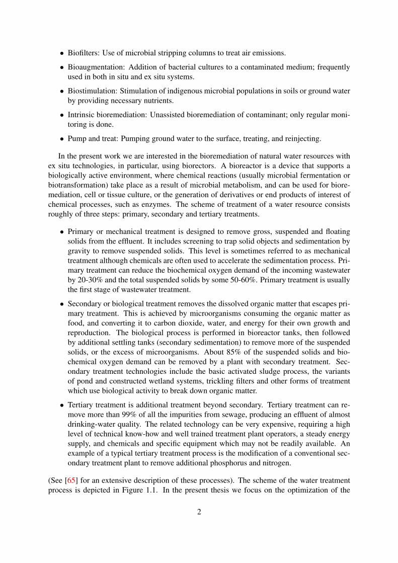
• Biofilters: Use of microbial stripping columns to treat air emissions.

• Bioaugmentation: Addition of bacterial cultures to a contaminated medium; frequentlyused in both in situ and ex situ systems.

• Biostimulation: Stimulation of indigenous microbial populations in soils or ground waterby providing necessary nutrients.

• Intrinsic bioremediation: Unassisted bioremediation of contaminant; only regular moni-toring is done.

• Pump and treat: Pumping ground water to the surface, treating, and reinjecting.

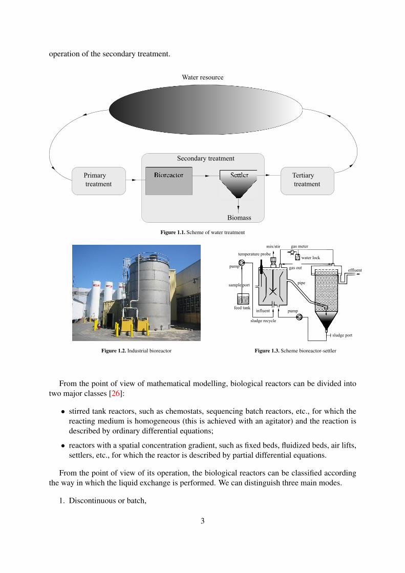
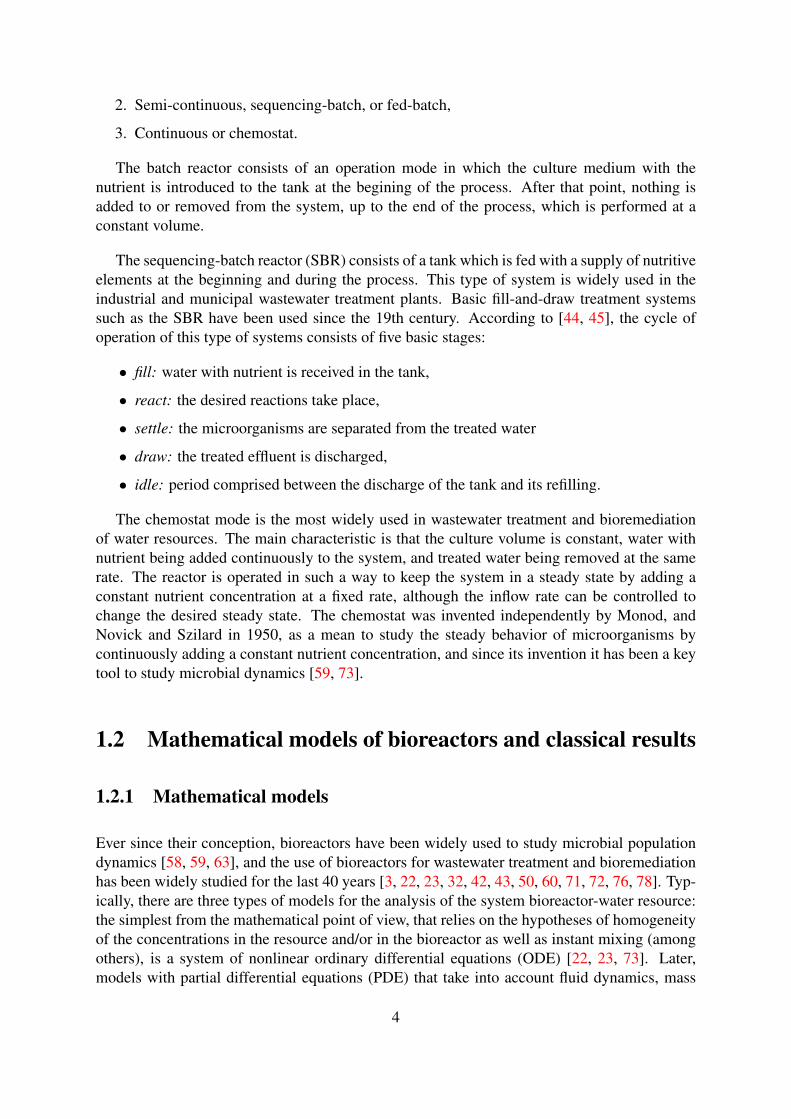
In the present work we are interested in the bioremediation of natural water resources withex situ technologies, in particular, using biorectors. A bioreactor is a device that supports abiologically active environment, where chemical reactions (usually microbial fermentation orbiotransformation) take place as a result of microbial metabolism, and can be used for biore-mediation, cell or tissue culture, or the generation of derivatives or end products of interest ofchemical processes, such as enzymes. The scheme of treatment of a water resource consistsroughly of three steps: primary, secondary and tertiary treatments.

• Primary or mechanical treatment is designed to remove gross, suspended and floatingsolids from the effluent. It includes screening to trap solid objects and sedimentation bygravity to remove suspended solids. This level is sometimes referred to as mechanicaltreatment although chemicals are often used to accelerate the sedimentation process. Pri-mary treatment can reduce the biochemical oxygen demand of the incoming wastewaterby 20-30% and the total suspended solids by some 50-60%. Primary treatment is usuallythe first stage of wastewater treatment.

• Secondary or biological treatment removes the dissolved organic matter that escapes pri-mary treatment. This is achieved by microorganisms consuming the organic matter asfood, and converting it to carbon dioxide, water, and energy for their own growth andreproduction. The biological process is performed in bioreactor tanks, then followedby additional settling tanks (secondary sedimentation) to remove more of the suspendedsolids, or the excess of microorganisms. About 85% of the suspended solids and bio-chemical oxygen demand can be removed by a plant with secondary treatment. Sec-ondary treatment technologies include the basic activated sludge process, the variantsof pond and constructed wetland systems, trickling filters and other forms of treatmentwhich use biological activity to break down organic matter.

• Tertiary treatment is additional treatment beyond secondary. Tertiary treatment can re-move more than 99% of all the impurities from sewage, producing an effluent of almostdrinking-water quality. The related technology can be very expensive, requiring a highlevel of technical know-how and well trained treatment plant operators, a steady energysupply, and chemicals and specific equipment which may not be readily available. Anexample of a typical tertiary treatment process is the modification of a conventional sec-ondary treatment plant to remove additional phosphorus and nitrogen.

(See [65] for an extensive description of these processes). The scheme of the water treatmentprocess is depicted in Figure 1.1. In the present thesis we focus on the optimization of the

2

operation of the secondary treatment.

Tertiary

treatment

Primary

treatment

Water resource

Biomass

Secondary treatment

Figure 1.1. Scheme of water treatment

Figure 1.2. Industrial bioreactor Figure 1.3. Scheme bioreactor-settler

From the point of view of mathematical modelling, biological reactors can be divided intotwo major classes [26]:

• stirred tank reactors, such as chemostats, sequencing batch reactors, etc., for which thereacting medium is homogeneous (this is achieved with an agitator) and the reaction isdescribed by ordinary differential equations;

• reactors with a spatial concentration gradient, such as fixed beds, fluidized beds, air lifts,settlers, etc., for which the reactor is described by partial differential equations.

From the point of view of its operation, the biological reactors can be classified accordingthe way in which the liquid exchange is performed. We can distinguish three main modes.

1. Discontinuous or batch,

3

2. Semi-continuous, sequencing-batch, or fed-batch,

3. Continuous or chemostat.

The batch reactor consists of an operation mode in which the culture medium with thenutrient is introduced to the tank at the begining of the process. After that point, nothing isadded to or removed from the system, up to the end of the process, which is performed at aconstant volume.

The sequencing-batch reactor (SBR) consists of a tank which is fed with a supply of nutritiveelements at the beginning and during the process. This type of system is widely used in theindustrial and municipal wastewater treatment plants. Basic fill-and-draw treatment systemssuch as the SBR have been used since the 19th century. According to [44, 45], the cycle ofoperation of this type of systems consists of five basic stages:

• fill: water with nutrient is received in the tank,

• react: the desired reactions take place,

• settle: the microorganisms are separated from the treated water

• draw: the treated effluent is discharged,

• idle: period comprised between the discharge of the tank and its refilling.

The chemostat mode is the most widely used in wastewater treatment and bioremediationof water resources. The main characteristic is that the culture volume is constant, water withnutrient being added continuously to the system, and treated water being removed at the samerate. The reactor is operated in such a way to keep the system in a steady state by adding aconstant nutrient concentration at a fixed rate, although the inflow rate can be controlled tochange the desired steady state. The chemostat was invented independently by Monod, andNovick and Szilard in 1950, as a mean to study the steady behavior of microorganisms bycontinuously adding a constant nutrient concentration, and since its invention it has been a keytool to study microbial dynamics [59, 73].

1.2 Mathematical models of bioreactors and classical results

1.2.1 Mathematical models

Ever since their conception, bioreactors have been widely used to study microbial populationdynamics [58, 59, 63], and the use of bioreactors for wastewater treatment and bioremediationhas been widely studied for the last 40 years [3, 22, 23, 32, 42, 43, 50, 60, 71, 72, 76, 78]. Typ-ically, there are three types of models for the analysis of the system bioreactor-water resource:the simplest from the mathematical point of view, that relies on the hypotheses of homogeneityof the concentrations in the resource and/or in the bioreactor as well as instant mixing (amongothers), is a system of nonlinear ordinary differential equations (ODE) [22, 23, 73]. Later,models with partial differential equations (PDE) that take into account fluid dynamics, mass

4

conservation and pollutant diffusion have been introduced to address the inhomogeneity of thepollutant in the resource [4] or the bioreactor vessel [24, 25]; this effect naturally appears due tothe speed of the reactions in the bioreactor and the slow diffusion speed as well as the slow mix-ing in large water resources; this is typically the situation of large scale reactors or large scalewater resources, fluidized beds, settlers among others. The third kind of models are the stochas-tic models, that take into account the uncertainty of different types of variables[14, 15, 20, 41].

Establishing a mathematical model for the dynamics in a bioreactor is not a simple task be-cause of the large number of interconnected variables involved in the process, for instance, pH,temperature, aereation, nutrient, different bacterial species and nutrient substances, end prod-ucts, etc. Thus, the choice of the number of reactions to be considered and components whichintervene in these reactions is very important for modeling. It will be carried out based on theknowledge that we have on the process and measurements which could have been carried out.The reaction scheme conditions the structure of the model. It will thus have to be chosen withparsimony, bearing in mind the objectives of the model and the precision which is expected.The required number of reactions and the reaction scheme can be determined directly from aset of available experimental data [26].

The mathematical model of the dynamics in the stirred tank reactor rely on the main conceptof mass balance [26, 27, 73], which can be broadly expressed as

Time variationof the mass

of the componentin the tank

=Mass of the

component enteringthe tank

−Mass of the

component leavingthe tank

+Mass of the

component producedby the reaction

−Mass of the

component consumedby the reaction

.

(1.1)

Suppose that X denotes a microbial species that will degrade a substrate denoted by S. Thisreaction is schematically described in the following form:

Sr(·)−→ X. (1.2)

in which X plays the role of an autocatalyst, i.e., it is both a product and a catalyst. The rateat which the process occurs is related to enzyme kinetics, and depends on the concentrationof substrate and biomass. Typically, the reaction rate r(·) is linear with respect to the biomassX , and it is assumed that microorganisms have uniform access to the substrate. With theseassumptions, the reaction rate has the form r(S,X) = µ(S)X , where the function µ(·) is calledthe specific growth rate [27]. In practice, growth rate functions are obtained experimentally inlaboratories.

There are two widely used expressions for the growth function µ(·). The first expression,due experimental works of Monod [58, 59], is also called Michaelis-Menten formulation (fromenzyme dynamics), has the form

µ(s) =µmaxs

KS + s. (1.3)

In (1.3), µmax is the maximum specific growth rate (in units of [1/h]) and KS is the half-saturation constant (in units of [g/l]). This formula models the saturation or limited growth

5

with respect to the substrate.

The second expression for the growth function takes into account the effect of inhibition ofthe growth of the microbial specie with respect to the excess of substrate. This expression iscalled the Haldane growth law:

µ(s) =µs

KS + s+ s2

Kl

. (1.4)

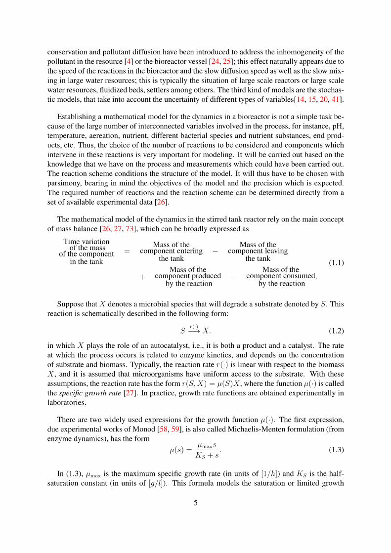
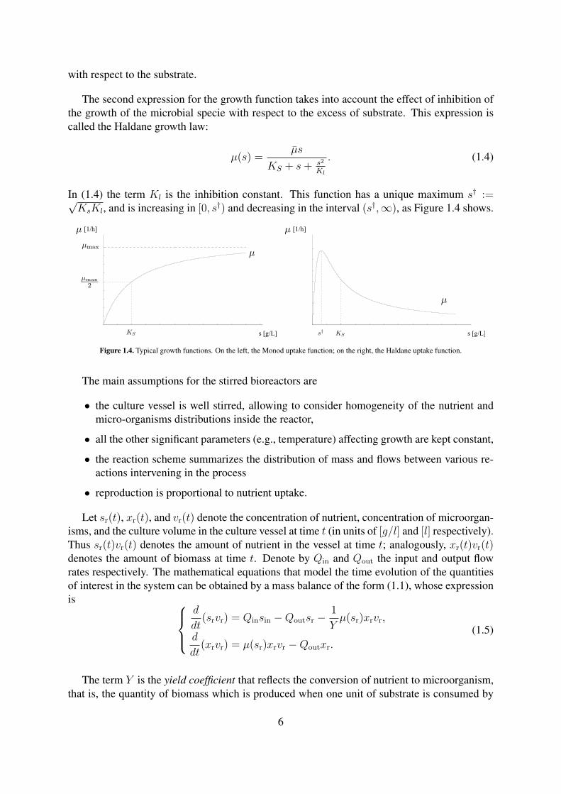
In (1.4) the term Kl is the inhibition constant. This function has a unique maximum s† :=√KsKl, and is increasing in [0, s†) and decreasing in the interval (s†,∞), as Figure 1.4 shows.

s [g/L]

[1/h] [1/h]

s [g/L]

Figure 1.4. Typical growth functions. On the left, the Monod uptake function; on the right, the Haldane uptake function.

The main assumptions for the stirred bioreactors are

• the culture vessel is well stirred, allowing to consider homogeneity of the nutrient andmicro-organisms distributions inside the reactor,

• all the other significant parameters (e.g., temperature) affecting growth are kept constant,

• the reaction scheme summarizes the distribution of mass and flows between various re-actions intervening in the process

• reproduction is proportional to nutrient uptake.

Let sr(t), xr(t), and vr(t) denote the concentration of nutrient, concentration of microorgan-isms, and the culture volume in the culture vessel at time t (in units of [g/l] and [l] respectively).Thus sr(t)vr(t) denotes the amount of nutrient in the vessel at time t; analogously, xr(t)vr(t)denotes the amount of biomass at time t. Denote by Qin and Qout the input and output flowrates respectively. The mathematical equations that model the time evolution of the quantitiesof interest in the system can be obtained by a mass balance of the form (1.1), whose expressionis

d

dt(srvr) = Qinsin −Qoutsr −

1

Yµ(sr)xrvr,

d

dt(xrvr) = µ(sr)xrvr −Qoutxr.

(1.5)

The term Y is the yield coefficient that reflects the conversion of nutrient to microorganism,that is, the quantity of biomass which is produced when one unit of substrate is consumed by

6

the reaction (1.2); it is assumed to be constant. Along with the mass balance equations weconsider the variation of culture volume given by the equation

d

dtvr = Qin −Qout. (1.6)

Finally, the expression of the equations of the bioreactor issr = − 1

Yµ(sr)xr +

Qin

vr

(sin − sr),

xr = µ(sr)xr −Qin

vr

xr,

vr = Qin −Qout.

(1.7)

According to the operation mode, the inflow and outflow rates are

• Batch: Qin = Qout = 0.

• SBR: Qout = 0.

• Chemostat: Qin = Qout.

1.2.2 Classical results on chemostats

Chemostats have been the object of extensive studies since the early works of Monod in the40’s [58] and its work La technique de la culture continue [59], the contributions of Novickand Szilard [63] in 1950, and Herbert et al [37] in 1956. In [73] there is an extensive study ofthe chemostat with the main mathematical results up to 1995.

Let us remind that for the chemostat the culture volume is constant, so the input flow rateQin and output flow rate Qout are equal at every time instant. Replacing in (1.2.2), we obtainthe simple model of chemostat

xr =

(µ(sr)−

Qin

vr

)xr,

sr = − 1

Yµ(sr)xr +

Qin

vr

(sin − sr).

(1.8)

The quantity D := Qin/vr is called dilution rate or washout rate; it has units of 1/t. Underan appropriate change of variable (xr = xr/Y , but we choose to keep xr instead of xr asvariable), the equations of the chemostat take the form

xr = (µ(sr)−D)xr,

sr = −µ(sr)xr +D(sin − sr).(1.9)

7

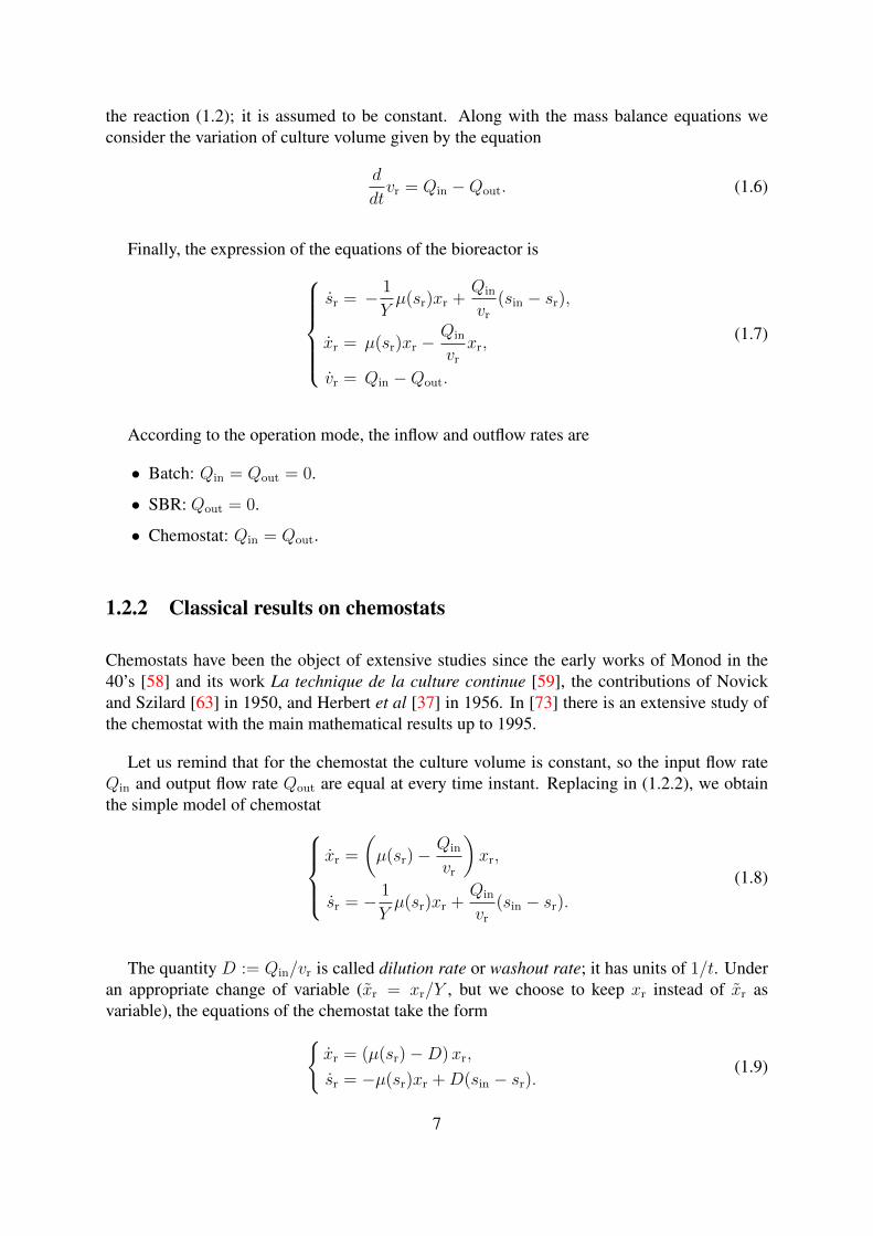
A basic mathematical result on the chemostat concerns the asymptotic behavior of the sys-tem. Depending on the behavior of the growth function and the dilution rate, there may existsa unique or several equilibrium points. Suppose that the chemostat is operated at a constantdilution rate D > 0. The trivial equilibrium point E0 := (0, sin) is called the washout. Thisequilibrium, in which there are no microorganisms in the reactor, is not desirable from the pointof view of the depollution process. The other equilibrium points are the solutions of the systemof equations

µ(s?r ) = D, x?r = sin − s?r . (1.10)

We notice that all the equilibrium points rely on the straight line xr +sr = sin. Indeed, this isstated by the second equation of (1.10), provided that D > 0. In Figure 1.5 we show the phaseportrait of the single species chemostat model with a Monod growth function with µmax = 1,KS = 1, sin = 4, for different dilution coefficients D ∈ [0, 1].

0 0.5 1 1.5 2 2.5 3 3.5 4 4.5 5

0

0.5

1

1.5

2

2.5

3

3.5

4

4.5

5

sr

xr

Phase portrait, D=0.05

0 0.5 1 1.5 2 2.5 3 3.5 4 4.5 5

0

0.5

1

1.5

2

2.5

3

3.5

4

4.5

5

sr

xr

Phase portrait, D=0.5

0 0.5 1 1.5 2 2.5 3 3.5 4 4.5 5

0

0.5

1

1.5

2

2.5

3

3.5

4

4.5

5

sr

xr

Phase portrait, D=0.75

0 0.5 1 1.5 2 2.5 3 3.5 4 4.5 5

0

0.5

1

1.5

2

2.5

3

3.5

4

4.5

5

sr

xr

Phase portrait, D=0.99

Figure 1.5. Trajectories on the phase portrait, depending on the diffusion parameterD. In green, the washout equilibrium; in red, the nontrivialequilibrium.

The following proposition summarizes the properties of the equilibrium points.

Proposition 1.1 Suppose that the constant dilution rate D > 0 is such that the equationµ(s?r ) = D has a solution s?r ∈ (0, sin).

• The equilibrium point E0 always exists (independently of D) and it is unstable.

• For all s?r < sin solution of µ(s?r ) = D there exists an equilibrium point E1 := (x?r , s?r ) =

(sin − s?r , s?r ). Any of these equilibrium points is locally asymptotically stable if µ′(s?r ) >0; if µ′(s?r ) ≤ 0 the equilibrium point is unstable.

The proof of this proposition relies on the eigenvalues of the Jacobian matrix of the system(1.9). Notice that we need to impose the condition s?r ∈ [0, sin] not just for mathematicalreasons but for the interpretation of the variables; indeed, the concentration of biomass at theequilibrium is x?r = sin−s?r , which only has a biological meaning if it is a nonnegative quantity.

For different types of uptake functions µ(·), Proposition 1.1 gives different qualitative re-

8

sults.

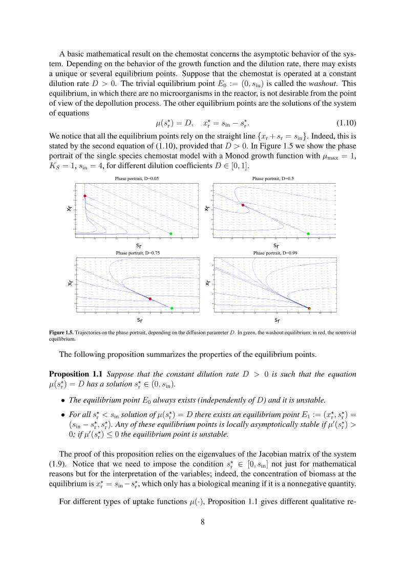
• For an increasing growth function (like the Monod’s law), if µ(sin) < D, the uniquelocally asymptotically stable equilibrium point is the washout. On the other hand, forD < µ(sin), there exits a unique solution to the equation µ(s?r ) = D in the interval(0, sin); the washout becomes unstable, and the point (x?r , s

?r ) = (sin−µ−1(D), µ−1(D))

is locally asymptotically stable (see Figure 1.6).

s [g/l]sin

[1/h]

D1

D2

(sin)

Figure 1.6. Equilibrium points for the Monod growth function. We see thatD1 < µmax, and then the concentration of substrate at equilibriumis s†r = λ1. For D2, the equilibrium is the washout.

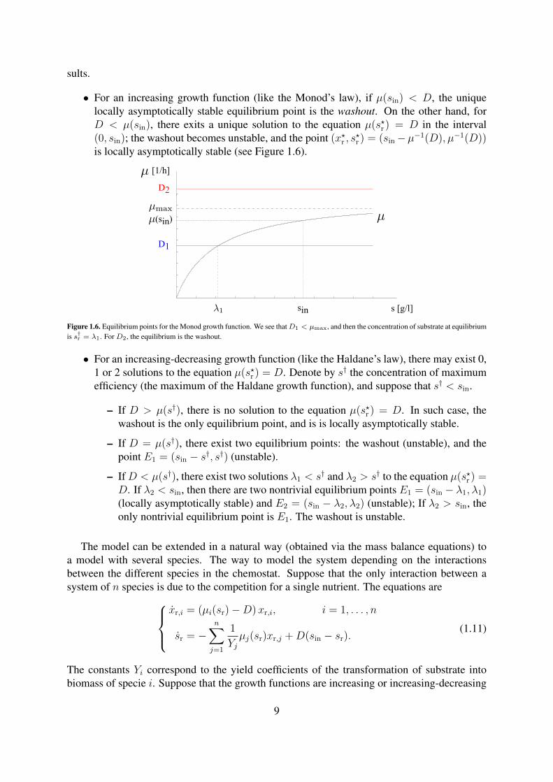
• For an increasing-decreasing growth function (like the Haldane’s law), there may exist 0,1 or 2 solutions to the equation µ(s?r ) = D. Denote by s† the concentration of maximumefficiency (the maximum of the Haldane growth function), and suppose that s† < sin.

– If D > µ(s†), there is no solution to the equation µ(s?r ) = D. In such case, thewashout is the only equilibrium point, and is is locally asymptotically stable.

– If D = µ(s†), there exist two equilibrium points: the washout (unstable), and thepoint E1 = (sin − s†, s†) (unstable).

– IfD < µ(s†), there exist two solutions λ1 < s† and λ2 > s† to the equation µ(s?r ) =D. If λ2 < sin, then there are two nontrivial equilibrium points E1 = (sin − λ1, λ1)(locally asymptotically stable) and E2 = (sin − λ2, λ2) (unstable); If λ2 > sin, theonly nontrivial equilibrium point is E1. The washout is unstable.

The model can be extended in a natural way (obtained via the mass balance equations) toa model with several species. The way to model the system depending on the interactionsbetween the different species in the chemostat. Suppose that the only interaction between asystem of n species is due to the competition for a single nutrient. The equations are

xr,i = (µi(sr)−D)xr,i, i = 1, . . . , n

sr = −n∑j=1

1

Yjµj(sr)xr,j +D(sin − sr).

(1.11)

The constants Yi correspond to the yield coefficients of the transformation of substrate intobiomass of specie i. Suppose that the growth functions are increasing or increasing-decreasing

9

[1/h]

s [g/l]

D3

D2

D1

sin

(sin)

Figure 1.7. Equilibrium points for the Haldane growth function. We see that for D1 < µ(s†) there exist two equilibrium points λ1 (locallyasymptotically stable) and λ2 (unstable) besides the washout (unstable). ForD2 = µ(s†) the equilibrium concentration is s?r = s† (unstable),and the washout is unstable. For D3, the equilibrium is the washout (stable).

(like Monod’s or Haldane’s law). Define, for each i ∈ 1, . . . , n, the set Λi(D) := sr >0 |µi(sr) > D. Because of the assumptions on the growth functions, if Λi(D) is not empty,then it is an interval Λi(D) = (λi, νi), where νi can take the value +∞. Suppose the particularsituation in which that all the λi’s that are finite and different, and without loss of generality, thatthe numbers λ1, . . . , λn are ordered such that 0 < λ1 < · · · < λm < sin < λm+1 < · · · < λnfor some m ∈ 1, . . . , n. The equilibrium points of this system are

• the washout: E0 = (s?r , x?r,1, . . . , x

?r,n) = (sin, 0, . . . , 0);

• Ei = (s?r , x?r,1, . . . , x

?r,n) = (λi, 0, . . . , Yi(sin − λi), . . . , 0) for i = 1, . . . ,m (in this case,

there is only substrate and specie i; this point exists because λi < sin); for i > m, Eidoes not exist.

• Ei = (s?r , x?r,1, . . . , x

?r,n) = (νi, 0, . . . , Yi(sin − νi), . . . , 0) for i = 1, . . . ,m ; (only sub-

strate and specie i), that exists only if νi < sin and in such case it is unstable. For i > m,Ei does not exist.

A well known result on the coexistence of several species in chemostats is the competitiveexclusion principle. This principle states that in a chemostat with constant operation parametersD and sin, several species cannot coexist [36, 73] (in a more general way, it states that whentwo species compete for the same critical resources within an environment, one of them willeventually outcompete and displace the other). This principle has a mathematical sustent in thework of [12] (as stated in [73]).

Theorem 1.2 ([12]) Define I = ∪i=1,...,m(λi, νi), with λi, νi as before. Suppose that I is anon-empty open interval. Then I = (λi, νj), for some j.

1. If λ1 < sin < νj , then E1 attracts all solutions with xr,i(0) > 0.

2. If sin > νj , then E0 and E1 are local attractors, their basins of attractions are non-empty open sets, and the complement of the union of the two basins of attraction has zeroLebesgue measure.

10

The first point of Theorem 1.2 corresponds to the competitive exclusion principle. Thesecond point of Theorem 1.2 states another phenomenon: the possibility that an excess ofnutrient can lead to the washout of all populations. Theorem 1.2 does not hold if some of theλi’s coincide.

Control problems arise naturally in the contex of biochemical processes, biotechnology, andwastewater treatment. Bioreactor control provides special challenges due to significant processvariability, the complexity of biological systems, the need, in many cases, to operate in a sterileenvironment, and the relatively few real-time direct measurements available that help definethe state of the culture. The study of control of the bioreactor is based on suitable manipulationof its operation parameters, the dilution rate, the input nutrient concentration, or the drop of thewell-mixed hypothesis. The first works on the control of chemostats address the problem ofcoexistence of different species under periodic changes on the dilution rate, when a fraction ofthe biomass and growing medium are periodically harvested, and when both the dilution rateand the concentration of the substrate in the feed are varied simultaneously and in a periodicmanner [13, 79].

Since the work by [22], the optimization of bioreactor operation has received great attentionin the literature, see [2, 3, 67] for reviews of the different optimization techniques that havebeen used in bioprocesses. Among them, the theory of optimal control has proven to be ageneric tool for deriving practical optimal rules [43, 71, 72].

Typically, the optimal control of continuous processes usually involves a two-step proce-dure. First, the optimal steady state is determined as a nominal set point that maximizes acriterion [76, 77]. The benefit of operating a periodic control about the nominal point can beanalyzed [1, 69]. Then, a control strategy that drives the state about the nominal set point fromany initial condition is searched for [50], possibly in the presence of model uncertainty usingextremum seeking techniques [6, 54, 84, 86].

1.2.3 Classical results on SBRs

SBRs are typically used to treat municipal and industrial wastewaters, particularly in areascharacterized by low or varying flow patterns. Improvements in equipment and technology,especially in aeration devices and computer control systems, have made SBRs a viable choiceover the conventional activated-sludge system. These plants are very practical for a number ofreasons. For instance, in areas where there is a limited amount of space, treatment takes place ina single basin instead of multiple basins, allowing for a smaller footprint. The treatment cyclecan be adjusted to undergo aerobic, anaerobic, and anoxic conditions in order to achieve bio-logical nutrient removal, including nitrification, denitrification, and some phosphorus removal.SBRs offer a cost-effective way to achieve lower effluent limits.

Flow-paced batch operation is generally preferable to time-paced batch or continuous inflowsystems. Under a flow-paced batch system, a plant receives the same volumetric loading andapproximately the same organic loading during every cycle. Under a time-paced mode, eachbasin receives different volumetric and organic loading during every cycle, and the plant is

11

not utilizing the full potential of this treatment method which is the ability to handle variablewaste streams. Time-paced operation can lead to under-treated effluent if the cycle time is notadjusted. For an SBR to be effective, the plant must have proper monitoring, allow operators toadjust the cycle time, and have knowledgeable operators who are properly trained to make thenecessary adjustments to the cycle [62].

Since the SBR is a time oriented system, the control objectives are usually to optimizetrajectories to attain a prescribed target in finite time [38, 45, 47, 51, 53, 70, 81] or to maximizeproduction at a given time [32, 55, 60, 78]. The single species model of SBR is

sr = − 1

Yµ(sr)xr +

u

vr

(sin − sr),

xr = µ(sr)xr −u

vr

xr,

vr = u,

(1.12)

where u is the inflow rate, that is usually the control variable and is bounded between 0 andumax. This system has the constraint that vr ≤ vmax.

In [60] the problem of attaining a prescribed pollution level sout with the tank at its maxi-mum capacity in minimal time is studied, for the single species case. The author considers avarying inflow substrate concentration sin to be a function of time. By means of Green theo-rem the optimal strategy is characterized in two cases depending on the behavior of the growthfunction. In the case that the growth function is monotone (Monod type), the optimal controlconsists on filling the tank at maximum speed u = umax until the tank is full v = vmax, and thenwait until sr ≤ sout. In the case that the growth function is nonmonotone with one maximum s†,the optimal strategy consists on a feedback control such that brings the pollutant concentrationsr as fast as possible to s† and to keep the system in that state up to the time when vr = vmax,and then wait.

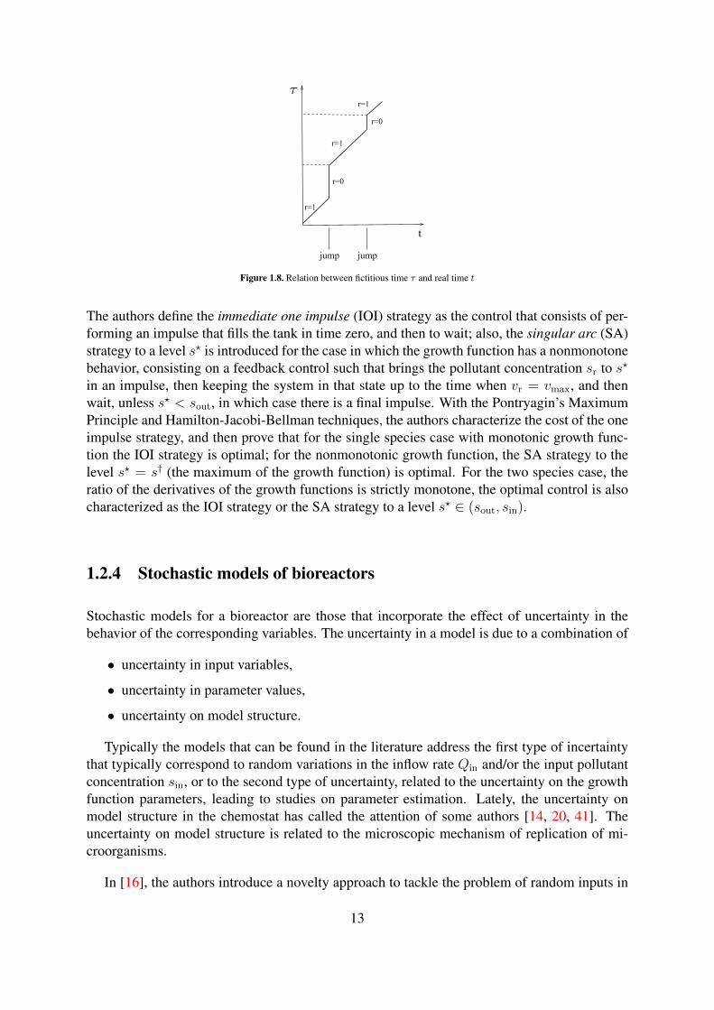
In [32], the authors extend the previous work to the case of several species and allowingimpulsional controls, that is, adding arbitrarily large amounts of water in arbitrarily small timeinstants. The SBR with impulse is modeled by a system of equations without impulse in afictitious time τ that allows to extend the real time t at the points where an impulse is made.

d

dτsr = −r

n∑j=1

1

Yjµj(sr)xr,j +

u

vr

(sin − sr),

d

dτxr,i = rµi(sr)xr,i −

u

vr

xr,i, i = 1, . . . , n,

d

dτvr = u,

(1.13)

Here, u is the control variable that represents the inflow rate, and r is a control variable thattakes the value 0 when there is an impulse (that lasts for the fictitious time intervals [τ0, τ1] suchthat

∫ τ1τ0u(τ) = v+ − v− explains the difference of volumes before and after the impulse) and

takes the value 1 otherwise. The behavior of the real time t as a function of τ is shown in Figure1.8

12

r=0

r=0

r=1

r=1

r=1

jump jump

t

Figure 1.8. Relation between fictitious time τ and real time t

The authors define the immediate one impulse (IOI) strategy as the control that consists of per-forming an impulse that fills the tank in time zero, and then to wait; also, the singular arc (SA)strategy to a level s? is introduced for the case in which the growth function has a nonmonotonebehavior, consisting on a feedback control such that brings the pollutant concentration sr to s?

in an impulse, then keeping the system in that state up to the time when vr = vmax, and thenwait, unless s? < sout, in which case there is a final impulse. With the Pontryagin’s MaximumPrinciple and Hamilton-Jacobi-Bellman techniques, the authors characterize the cost of the oneimpulse strategy, and then prove that for the single species case with monotonic growth func-tion the IOI strategy is optimal; for the nonmonotonic growth function, the SA strategy to thelevel s? = s† (the maximum of the growth function) is optimal. For the two species case, theratio of the derivatives of the growth functions is strictly monotone, the optimal control is alsocharacterized as the IOI strategy or the SA strategy to a level s? ∈ (sout, sin).

1.2.4 Stochastic models of bioreactors

Stochastic models for a bioreactor are those that incorporate the effect of uncertainty in thebehavior of the corresponding variables. The uncertainty in a model is due to a combination of

• uncertainty in input variables,

• uncertainty in parameter values,

• uncertainty on model structure.

Typically the models that can be found in the literature address the first type of incertaintythat typically correspond to random variations in the inflow rate Qin and/or the input pollutantconcentration sin, or to the second type of uncertainty, related to the uncertainty on the growthfunction parameters, leading to studies on parameter estimation. Lately, the uncertainty onmodel structure in the chemostat has called the attention of some authors [14, 20, 41]. Theuncertainty on model structure is related to the microscopic mechanism of replication of mi-croorganisms.

In [16], the authors introduce a novelty approach to tackle the problem of random inputs in

13

the model of chemostat, particularly the random nutrient supplying rate or the random inputnutrient concentration, with or without wall growth, from the mathematical point of view ofrandom dynamical systems and using the concept of random attractors. The authors obtain re-sults of existence of uniformly bounded non-negative solutions, existence of random attractors,and geometric details of random attractors for different values of parameters.

In [41], the authors model the influence of random fluctuations by setting up and analyz-ing a stochastic differential equation, and show that random effects may lead to extinction inscenarios where the deterministic model predicts persistence, and establish some stochasticpersistence results. The single species model presented in that article is

dX0 = (r − δX0 − a(X0, X1))dt+ σ0X0dW0(t),

dX1 = (a(X0, X1)− s(X1))dt+ σ1X1dW1(t),(1.14)

where X0 stands for substrate concentration, X1 denotes the biomass concentration of a mi-crobe species feeding on the substrate; the substrate inflow rate r and the relative substrateoutflow rate δ are positive constants; the substrate uptake rate a(X0, X1) = µ(X0)X1, which isequal to the microbe growth rate, is non-negative and strictly increasing in both variables, witha(X0, 0) = a(0, X1) = 0 for all X0, X1 (this means that substrate uptake occurs only whensubstrate and microbes are present); the microbe removal rate s(x1) is non-negative and strictlyincreasing; and σ0, σ1 ≥ reflect the size of the stochastic effects. The derivation of said modelis performed as a limit of a family of discrete Markov Chains whose random effects dependlinearly on the respective variable. The authors prove that under suitable assumptions for everyinitial condition the equation (1.14) has a strong solution defined for every time instant, path-wise uniqueness holds, and with probability one the process stays in the interior of the positiveorthant.

In [14], the authors propose a model of chemostat where the bacterial population is individually-based, each bacterium is explicitly represented and has a mass evolving continuously overtime. The substrate concentration is represented as a conventional ordinary differential equa-tion. These two components are coupled with the bacterial consumption. Mechanisms actingon the bacteria such as growth, division and washout, are explicitly described, and bacteriainteract via consumption. The authors prove the convergence of this process to the solution ofan integro-differential equation when the population size tends to infinity. The equations of themodel are

Yt =1

vr

∫ mmax

0

xpt(x)dx,

St = D(sin − St)−k

vr

∫ mmax

0

ρ(St, x)pt(x)dx,

∂

∂tpt(x) +

∂

∂x(ρ(St, x)pt(x)) + (λ(St, x) +D)pt(x) = 2

∫ mmax

0

λ(St, z)

zq(xz

)pt(z)dz,

for x ∈ [0,mmax]. Here pt(x) is the density of population with respect to its mass at a time t.Hence

∫ m1

m0pt(x)dx is the number of cells which mass is between m0 and m1 and the average

biomass concentration at time t is Yt; ρ(s, x) and λ(s, x) are respectively the growth func-tion and the division rate of a bacterium of mass x with a substrate concentration s (typically

14

ρ(s, x) = µ(s)x), the mass distribution of the daughter cells is represented by the probabilitydensity function q(α) on [0, 1].

In [20], the authors introduce two stochastic chemostat models consisting of a coupledpopulation-nutrient process reflecting the interaction between the nutrient and the bacteria inthe chemostat with finite volume, where the nutrient concentration evolves continuously butdepends on the population size, while the population size is a birth-and-death process with co-efficients depending on time through the nutrient concentration. The nutrient is shared by thebacteria and creates a regulation of the bacterial population size. The latter and the fluctuationsdue to the random births and deaths of individuals make the population go almost surely toextinction. The authors study the long-time behavior of the bacterial population conditionedto non-extinction, prove the global existence of the process and its almost-sure extinction; theexistence of quasi-stationary distributions is obtained based on a general fixed-point argument.The authors also prove the absolute continuity of the nutrient distribution when conditioned toa fixed number of individuals and the smoothness of the corresponding densities. The equationof the substrate concentration is given by

d

dtS(t) = D(sin − S(t))− b(S(t))N(t),

linked to the process of the population size by the infinitesimal generator [30] of the processZ = (Z(t) := (N(t), S(t)), t ≥ 0) given by

L f(n, s) = b(s)nf(n+ 1, s) + (D + d(s))nf(n− 1, s)− (b(s) +D + d(s))nf(n, s)

+ (D(sin − s)− nb(s))∂

∂sf(n, s).

In this model b(d) is the birthe rate per individual (typically the Monod growth function) andd(s) is the background death rate per individual, that depends on the nutrient. In this model itis important to remark the fact that there is almost sure extinction of the biomass, which is aresult that does not hold for the deterministic models.

1.3 Model of inhomogeneous lake

This thesis studies the bioremediation of natural water reservoirs, such as lakes, ponds, lagoons,underground waters, water tables, etc., with the use of a bioreactor. From a mathematical pointof view, this means that we couple the dynamics of a bioreactor with the dynamics of thepollutant concentration in the water resource. We suppose that there is a settler that perfectlyseparates the biomass from the effluent of the bioreactor in negligible time before returning thetreated water to the resource.

Since typically water resources have a large volume and spatial constraints, inhomogeneityof the distribution of the pollutant in the resource naturally arises. The connection between thebioreactor and the water reservoir induces water movements in the latter. We model the waterresource as a bounded open domain Ω ⊆ Rn, with n = 2 for lakes of small depth, or n = 3

15

for a deep lake. We suposse that the velocity field ~v(t, x) depends only of the inflow/outflowdischarges from the bioreactor, the water viscosity is constant and homogeneous, and the fluidis incompressible. Denote Γin ⊆ ∂Ω is the area that receives the effluent of the reactor andΓout ⊆ ∂Ω is the area from which water is taken to the bioreactor. Denote p the pressure of thefluid. The equations that model the velocity field in the resource are given by the Navier-Stokesequations of an incompressible fluid [4]:

∂

∂t~v + ~v · ∇~v +∇p− νv∆v = 0, (t, x) ∈ (0,∞)× Ω,

∇ · ~v = 0, (t, x) ∈ (0,∞)× Ω.(1.15)

With this equations we provide the initial condition

~v(t = 0, x) = 0, x ∈ Ω,

and the boundary conditions for Γin, Γout, and Γ0 := ∂Ω\(Γin ∪ Γout):~v(t, x) = Q(t)~vin(x), x ∈ Γin,

~v(t, x) = Q(t)~vout(x), x ∈ Γout,

~v(t, x) = 0, x ∈ Γ0.

The functions ~vin and ~vout are unitary parabolic vector fields that describe the velocity profileon Γin and Γout parallel to the outwards normal n and satisfy

−∫

Γin

~vin · ndS =

∫Γout

~vout · ndS = 1.

The previous model allows to characterize the velocity field in the water resource as a func-tion of the pumping speed Q(t). Numerical simulations can be performed to compute the ve-locity field independently of the pollutant concentration (since we have assumed that changesin the pollutant concentration do not affect the viscosity of the fluid). If the resource has a largedepth, a 3 dimensional model can be considered. This is numerically costly because of the sizeas well as the geometry of the resource. If the depth is small, a 2 dimensional model gives goodresults.

Now, denote by sl(t, x) the concentration of pollutant in the resource at the point x ∈ Ω inthe time instant t. Suppose that the diffusivity coefficient νs of the pollutant is constant andhomogeneous. The equation that models the time evolution of the concentration of pollutantin the resource are composed by an equation of mass conservation of the pollutant (given thevelocity field ~v previously computed) are

∂

∂tsl − νs∆sl + ~v · ∇sl = 0, (t, x) ∈ (0,∞)× Ω, (1.16)

with the initial conditionsl(t = 0, x) = s0

l (x), x ∈ Ω,

16

and boundary conditions

νs∂sl∂n

(t, x) =Q(t)

|Γin|~vin(x) · n(sl(t, x)− sout

r (t)), x ∈ Γin,

∂sl∂n

(t, x) = 0, x ∈ Γout,

∂sl∂n

(t, x) = 0, x ∈ Γ0.

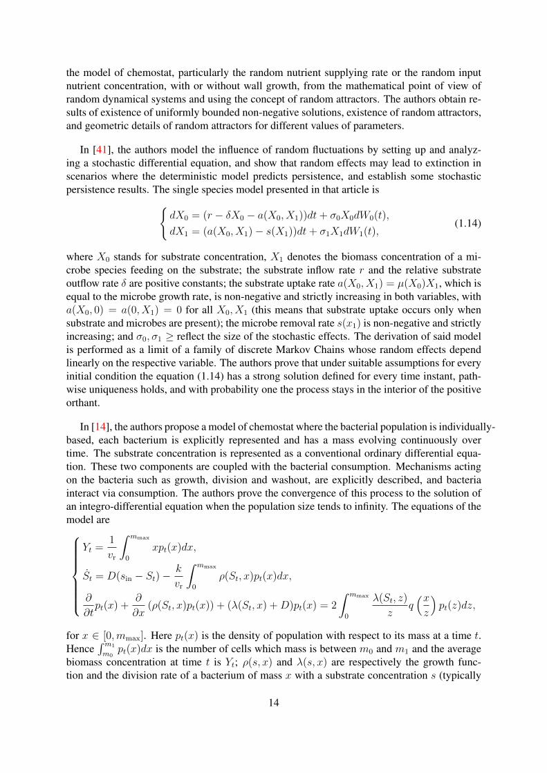
Numerical simulations of this model in [4] show that the inhomogeneity can be consideredas if there were two different zones: a first zone that is being actively treated by the bioreactorin which there could be considered a gradient of concentrations, and another zone that is beingdepolluted mainly by diffusion with the first zone. This amounts to consider simpler models fortreating the inhomogeneity of the pollutant, for instance, compartimental models that considerthe resource splitted into two or more zones, each of them with homogeneous concentration,and connected between each other by advection or diffusion coefficients according to geometricspecifications.

Figure 1.9. Behavior of the inhomogeneous representation of a lake. From the homogeneous initial distribution of pollutant (on the left), thesystem evolves up to a point in which two zones are clearly differentiated (on the right). Taken from [4]

The motivation of this part of the thesis is to establish optimal control rules for the depollu-tion of water resources in minimal time, with the use of simpler ODE models as an approxima-tion of the inhomogeneous model. In this regard, there exists a tradeoff between the pumpingspeed and the quality of depollution. On the one hand, if the pumping speed Q is too low, thequality of the depollution will be good but the treatment time will be long since it will take toomuch time to recirculate the water through the bioreactor. On the other hand, if the pumpingspeed is too high, the quality of the treatment in the reactor will be poor because the microor-ganisms do not have enough time to process the pollutant, and it could even lead to the washoutin the reactor. Finding an optimal control for minimal time treatment has both a biological andan economical sense. The problem of the depollution of water resources consists in treating theresource by means of a bioreactor by controlling the inflow rate Q and making the pollutantconcentration in the resource to decrease under a certain level s considered safe.

17

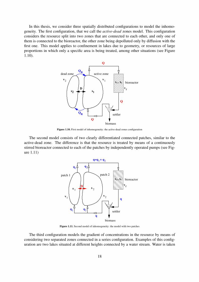
In this thesis, we consider three spatially distributed configurations to model the inhomo-geneity. The first configuration, that we call the active-dead zones model. This configurationconsiders the resource split into two zones that are connected to each other, and only one ofthem is connected to the bioreactor, the other zone being depolluted only by diffusion with thefirst one. This model applies to confinement in lakes due to geometry, or resources of largeproportions in which only a specific area is being treated, among other situations (see Figure1.10).

Q

s2 s1

1v

2v

rv

s , xrr bioreactor

biomass

settler

dead zone active zone

Q

Q

QR

QR

D

Figure 1.10. First model of inhomogeneity: the active-dead zones configuration

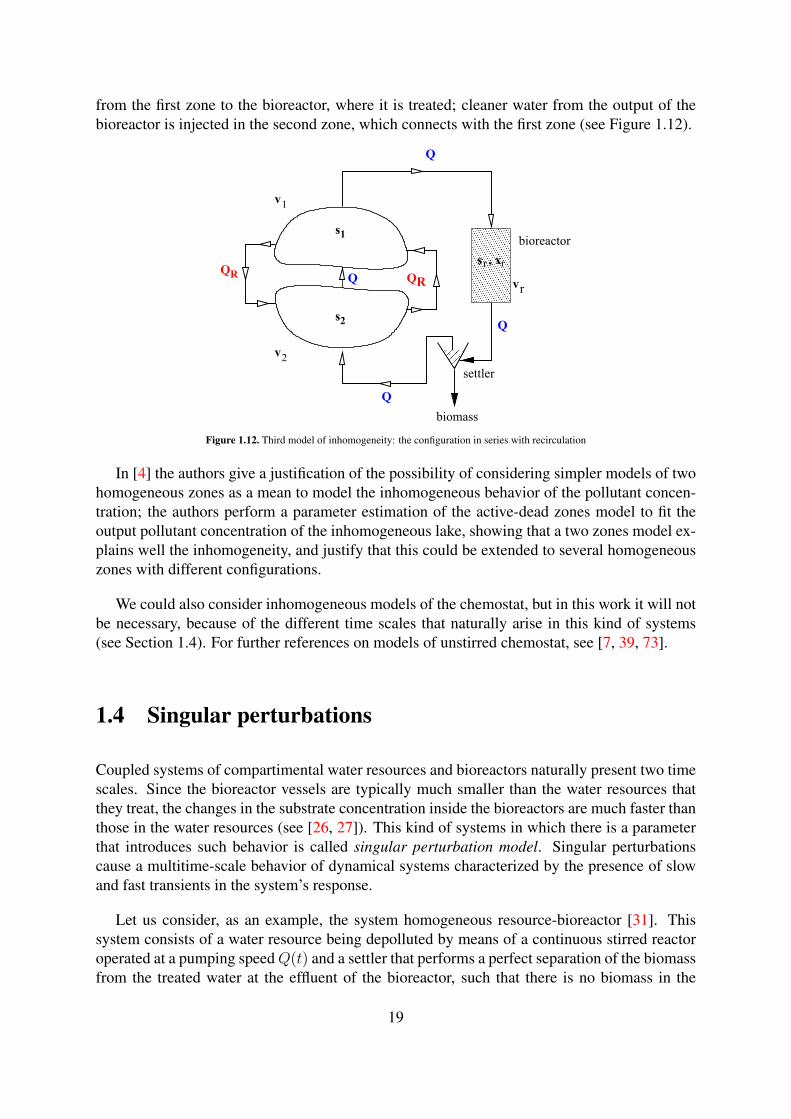
The second model consists of two clearly differentiated connected patches, similar to theactive-dead zone. The difference is that the resource is treated by means of a continuouslystirred bioreactor connected to each of the patches by independently operated pumps (see Fig-ure 1.11)

q1 q2

q=q + q1 2

1s 2s

2vv1

rv

s , xrr bioreactor

biomass

settler

q

patch 2patch 1

q1q

2

q

D

Figure 1.11. Second model of inhomogeneity: the model with two patches

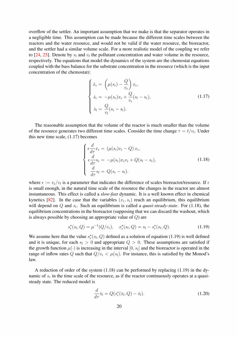
The third configuration models the gradient of concentrations in the resource by means ofconsidering two separated zones connected in a series configuration. Examples of this config-uration are two lakes situated at different heights connected by a water stream. Water is taken

18

from the first zone to the bioreactor, where it is treated; cleaner water from the output of thebioreactor is injected in the second zone, which connects with the first zone (see Figure 1.12).

Q

rv

s , xrr

biomass

Q

Q

bioreactor

settler

s2

1v

2v

Q QR

s1

QR

Figure 1.12. Third model of inhomogeneity: the configuration in series with recirculation

In [4] the authors give a justification of the possibility of considering simpler models of twohomogeneous zones as a mean to model the inhomogeneous behavior of the pollutant concen-tration; the authors perform a parameter estimation of the active-dead zones model to fit theoutput pollutant concentration of the inhomogeneous lake, showing that a two zones model ex-plains well the inhomogeneity, and justify that this could be extended to several homogeneouszones with different configurations.

We could also consider inhomogeneous models of the chemostat, but in this work it will notbe necessary, because of the different time scales that naturally arise in this kind of systems(see Section 1.4). For further references on models of unstirred chemostat, see [7, 39, 73].

1.4 Singular perturbations

Coupled systems of compartimental water resources and bioreactors naturally present two timescales. Since the bioreactor vessels are typically much smaller than the water resources thatthey treat, the changes in the substrate concentration inside the bioreactors are much faster thanthose in the water resources (see [26, 27]). This kind of systems in which there is a parameterthat introduces such behavior is called singular perturbation model. Singular perturbationscause a multitime-scale behavior of dynamical systems characterized by the presence of slowand fast transients in the system’s response.

Let us consider, as an example, the system homogeneous resource-bioreactor [31]. Thissystem consists of a water resource being depolluted by means of a continuous stirred reactoroperated at a pumping speedQ(t) and a settler that performs a perfect separation of the biomassfrom the treated water at the effluent of the bioreactor, such that there is no biomass in the

19

overflow of the settler. An important assumption that we make is that the separator operates ina negligible time. This assumption can be made because the different time scales between thereactors and the water resource, and would not be valid if the water resource, the bioreactor,and the settler had a similar volume scale. For a more realistic model of the coupling we referto [24, 25]. Denote by sl and vl the pollutant concentration and water volume in the resource,respectively. The equations that model the dynamics of the system are the chemostat equationscoupled with the bass balance for the substrate concentration in the resource (which is the inputconcentration of the chemostat):

xr =

(µ(sr)−

Q

vr

)xr,

sr = −µ(sr)xr +Q

vr

(sl − sr),

sl =Q

vl(sr − sl).

(1.17)

The reasonable assumption that the volume of the reactor is much smaller than the volumeof the resource generates two different time scales. Consider the time change τ = t/vl. Underthis new time scale, (1.17) becomes

εd

dτxr = (µ(sr)vr −Q)xr,

εd

dτsr = −µ(sr)xrvr +Q(sl − sr),

d

dτsl = Q(sr − sl).

(1.18)

where ε := vr/vl is a parameter that indicates the difference of scales bioreactor/resource. If εis small enough, in the natural time scale of the resource the changes in the reactor are almostinstantaneous. This effect is called a slow-fast dynamic. It is a well known effect in chemicalkynetics [82]. In the case that the variables (xr, sr) reach an equilibrium, this equilibriumwill depend on Q and sl. Such an equilibrium is called a quasi-steady-state. For (1.18), theequilibrium concentrations in the bioreactor (supposing that we can discard the washout, whichis always possible by choosing an appropriate value of Q) are

s?r (sl, Q) = µ−1(Q/vr), x?r (sl, Q) = sl − s?r (sl, Q). (1.19)

We assume here that the value s?r (sl, Q) defined as a solution of equation (1.19) is well definedand it is unique, for each sl > 0 and appropriate Q > 0. These assumptions are satisfied ifthe growth function µ(·) is increasing in the interval [0, sl] and the bioreactor is operated in therange of inflow rates Q such that Q/vr < µ(sl). For instance, this is satisfied by the Monod’slaw.

A reduction of order of the system (1.18) can be performed by replacing (1.19) in the dy-namic of sr in the time scale of the resource, as if the reactor continuously operates at a quasi-steady state. The reduced model is

d

dτsl = Q(s?r (sl, Q)− sl). (1.20)

20

The reduced model (1.20) is much simpler in mathematical terms than the original model(1.18) and can be seen as an approximation of the latter. The remaining question is relative tothe behavior of the approximated system with respect to the original one: Is it true that whenε approaches to 0, the solution of (1.18) approaches to the trajectory (xr, sr, sl), where sl(t) issolution of (1.20) and xr(t) = x?r (sl(t), Q), sr(t) = s?r (sl(t), Q)? The answer to that questionis given by Tychonnof theorem [49, Theorem 11.1]. This theorem states that the solution of asystem of the form

x = f(t, x, z, ε),

εz = g(t, x, z, ε),(1.21)

can be approximated by the solution of the reduced system˙x = f(t, x, h(t, x), 0),

z = h(t, x),(1.22)

when the perturbation ε converges to 0, where h(t, x) is a solution of g(t, x, h(t, x), 0) =0. More precisely, Tychonnof’s theorem states the following: consider any time interval[t0, t1], the singular perturbation problem (1.21), and let z = h(t, x) be an isolated root ofg(t, x, h(t, x), 0) = 0. Assume that the following conditions are satisfied for all (t, x, z −h(t, x), ε) ∈ [t0, t1] × Dx × Dy × [0, ε0], for some domains Dx ⊆ Rn convex and Dy ⊆ Rm

that contains the origin:

• the functions f , g, their first partial derivatives with respect to (x, z, ε), and the firstpartial derivative of g with respect to t are continuous; the functions (t, x) 7→ h(t, x) and(t, x, z) 7→ ∂g(t, x, z, 0)/∂z are differentiable with continuous derivatives;

• the reduced problem (1.22) has a unique solution x(t) ∈ S, t ∈ [t0, t1], with S compactsubset of Dx;

• the origin is an exponentially stable equilibrium of the equation

dy

dt(τ) = g(t, x, y(τ) + h(t, x), 0). (1.23)

uniformly in (t, x); letRy ⊆ Dy be the region of attraction of (1.23), and Ωy be a compactsubset ofRy.

Then, there exists a positive constant ε? > 0 such that for all initial condition z(0)−h(t0, x0) inΩy and 0 < ε < ε?, the singular problem (1.21) has a unique solution x(t, ε), z(t, ε) on [t0, t1]and

x(t, ε)− x(t) = O(ε),

z(t, ε)− h(t, x(t))− y(t/ε) = O(ε)(1.24)

holds uniformly for t ∈ [t0, t1], where y(τ) is solution of (1.23) with initial condition y(t0) =z(t0) − h(t0, x(t0)). Moreover, given any tb > t0 there exists another ε?? ≤ ε? such thatuniformly for t ∈ [tb, t1]

z(t, ε)− h(t, x(t)) = O(ε) (1.25)

whenever ε < ε??.

21

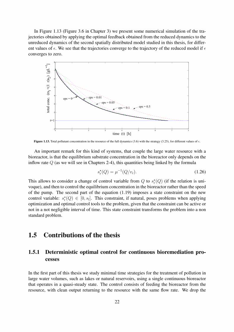
In Figure 1.13 (Figure 3.6 in Chapter 3) we present some numerical simulation of the tra-jectories obtained by applying the optimal feedback obtained from the reduced dynamics to theunreduced dynamics of the second spatially distributed model studied in this thesis, for differ-ent values of ε. We see that the trajectories converge to the trajectory of the reduced model if εconverges to zero.

0 1 2 3 4 5 6 7 80

2

3

4

5

6

7

8

time (t) [h]

tota

l co

nc.

(r

s 1+

(1r)

s 2)

[gL

1]

eps = 0 eps = 0.01

eps = 0.05

eps = 0.1 eps = 0.5

s=1

Figure 1.13. Total pollutant concentration in the resource of the full dynamics (3.6) with the strategy (3.25), for different values of ε.

An important remark for this kind of systems, that couple the large water resource with abioreactor, is that the equilibrium substrate concentration in the bioreactor only depends on theinflow rate Q (as we will see in Chapters 2-4), this quantities being linked by the formula

s?r (Q) = µ−1(Q/vr). (1.26)

This allows to consider a change of control variable from Q to s?r (Q) (if the relation is uni-voque), and then to control the equilibrium concentration in the bioreactor rather than the speedof the pump. The second part of the equation (1.19) imposes a state constraint on the newcontrol variable: s?r (Q) ∈ [0, sl]. This constraint, if natural, poses problems when applyingoptimization and optimal control tools to the problem, given that the constraint can be active ornot in a not negligible interval of time. This state constraint transforms the problem into a nonstandard problem.

1.5 Contributions of the thesis

1.5.1 Deterministic optimal control for continuous bioremediation pro-cesses

In the first part of this thesis we study minimal time strategies for the treatment of pollution inlarge water volumes, such as lakes or natural reservoirs, using a single continuous bioreactorthat operates in a quasi-steady state. The control consists of feeding the bioreactor from theresource, with clean output returning to the resource with the same flow rate. We drop the

22

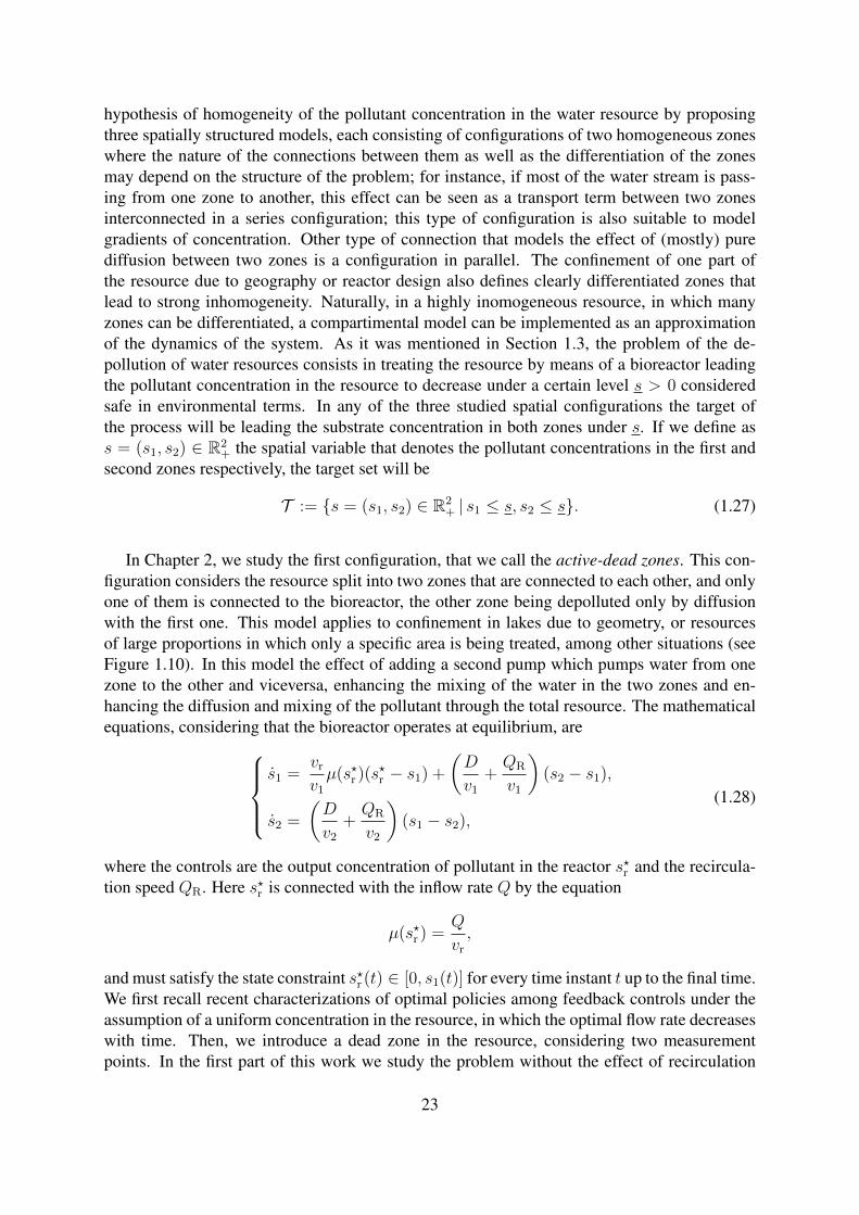
hypothesis of homogeneity of the pollutant concentration in the water resource by proposingthree spatially structured models, each consisting of configurations of two homogeneous zoneswhere the nature of the connections between them as well as the differentiation of the zonesmay depend on the structure of the problem; for instance, if most of the water stream is pass-ing from one zone to another, this effect can be seen as a transport term between two zonesinterconnected in a series configuration; this type of configuration is also suitable to modelgradients of concentration. Other type of connection that models the effect of (mostly) purediffusion between two zones is a configuration in parallel. The confinement of one part ofthe resource due to geography or reactor design also defines clearly differentiated zones thatlead to strong inhomogeneity. Naturally, in a highly inomogeneous resource, in which manyzones can be differentiated, a compartimental model can be implemented as an approximationof the dynamics of the system. As it was mentioned in Section 1.3, the problem of the de-pollution of water resources consists in treating the resource by means of a bioreactor leadingthe pollutant concentration in the resource to decrease under a certain level s > 0 consideredsafe in environmental terms. In any of the three studied spatial configurations the target ofthe process will be leading the substrate concentration in both zones under s. If we define ass = (s1, s2) ∈ R2

+ the spatial variable that denotes the pollutant concentrations in the first andsecond zones respectively, the target set will be

T := s = (s1, s2) ∈ R2+ | s1 ≤ s, s2 ≤ s. (1.27)

In Chapter 2, we study the first configuration, that we call the active-dead zones. This con-figuration considers the resource split into two zones that are connected to each other, and onlyone of them is connected to the bioreactor, the other zone being depolluted only by diffusionwith the first one. This model applies to confinement in lakes due to geometry, or resourcesof large proportions in which only a specific area is being treated, among other situations (seeFigure 1.10). In this model the effect of adding a second pump which pumps water from onezone to the other and viceversa, enhancing the mixing of the water in the two zones and en-hancing the diffusion and mixing of the pollutant through the total resource. The mathematicalequations, considering that the bioreactor operates at equilibrium, are

s1 =vr

v1

µ(s?r )(s?r − s1) +

(D

v1

+QR

v1

)(s2 − s1),

s2 =

(D

v2

+QR

v2

)(s1 − s2),

(1.28)

where the controls are the output concentration of pollutant in the reactor s?r and the recircula-tion speed QR. Here s?r is connected with the inflow rate Q by the equation

µ(s?r ) =Q

vr

,

and must satisfy the state constraint s?r (t) ∈ [0, s1(t)] for every time instant t up to the final time.We first recall recent characterizations of optimal policies among feedback controls under theassumption of a uniform concentration in the resource, in which the optimal flow rate decreaseswith time. Then, we introduce a dead zone in the resource, considering two measurementpoints. In the first part of this work we study the problem without the effect of recirculation

23

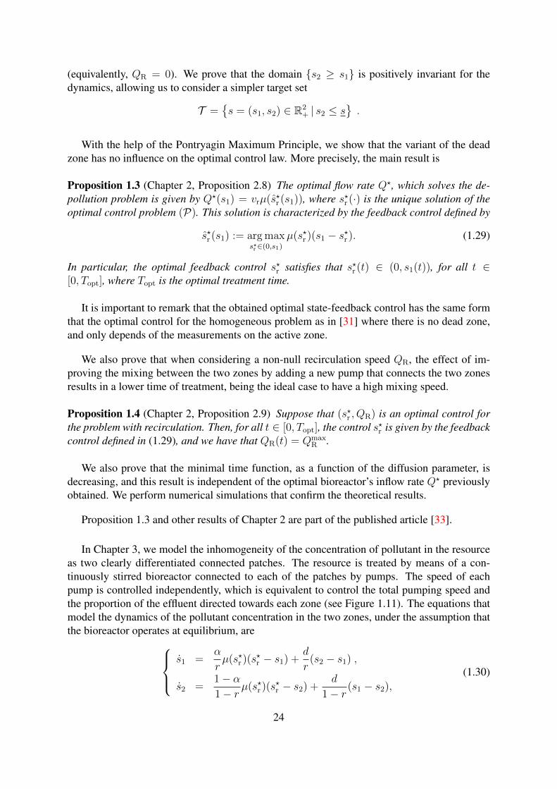
(equivalently, QR = 0). We prove that the domain s2 ≥ s1 is positively invariant for thedynamics, allowing us to consider a simpler target set

T =s = (s1, s2) ∈ R2

+ | s2 ≤ s.

With the help of the Pontryagin Maximum Principle, we show that the variant of the deadzone has no influence on the optimal control law. More precisely, the main result is

Proposition 1.3 (Chapter 2, Proposition 2.8) The optimal flow rate Q?, which solves the de-pollution problem is given by Q?(s1) = vrµ(s?r (s1)), where s?r (·) is the unique solution of theoptimal control problem (P). This solution is characterized by the feedback control defined by

s?r (s1) := arg maxs?r∈(0,s1)

µ(s?r )(s1 − s?r ). (1.29)

In particular, the optimal feedback control s?r satisfies that s?r (t) ∈ (0, s1(t)), for all t ∈[0, Topt], where Topt is the optimal treatment time.

It is important to remark that the obtained optimal state-feedback control has the same formthat the optimal control for the homogeneous problem as in [31] where there is no dead zone,and only depends of the measurements on the active zone.

We also prove that when considering a non-null recirculation speed QR, the effect of im-proving the mixing between the two zones by adding a new pump that connects the two zonesresults in a lower time of treatment, being the ideal case to have a high mixing speed.

Proposition 1.4 (Chapter 2, Proposition 2.9) Suppose that (s?r , QR) is an optimal control forthe problem with recirculation. Then, for all t ∈ [0, Topt], the control s?r is given by the feedbackcontrol defined in (1.29), and we have that QR(t) = Qmax

R .

We also prove that the minimal time function, as a function of the diffusion parameter, isdecreasing, and this result is independent of the optimal bioreactor’s inflow rate Q? previouslyobtained. We perform numerical simulations that confirm the theoretical results.

Proposition 1.3 and other results of Chapter 2 are part of the published article [33].

In Chapter 3, we model the inhomogeneity of the concentration of pollutant in the resourceas two clearly differentiated connected patches. The resource is treated by means of a con-tinuously stirred bioreactor connected to each of the patches by pumps. The speed of eachpump is controlled independently, which is equivalent to control the total pumping speed andthe proportion of the effluent directed towards each zone (see Figure 1.11). The equations thatmodel the dynamics of the pollutant concentration in the two zones, under the assumption thatthe bioreactor operates at equilibrium, are

s1 =α

rµ(s?r )(s?r − s1) +

d

r(s2 − s1) ,

s2 =1− α1− r

µ(s?r )(s?r − s2) +d

1− r(s1 − s2),

(1.30)

24

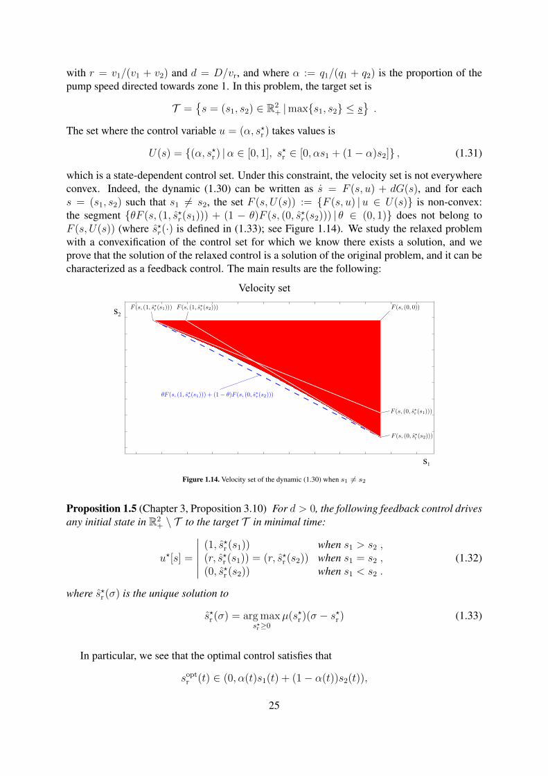
with r = v1/(v1 + v2) and d = D/vr, and where α := q1/(q1 + q2) is the proportion of thepump speed directed towards zone 1. In this problem, the target set is

T =s = (s1, s2) ∈ R2

+ |maxs1, s2 ≤ s.

The set where the control variable u = (α, s?r ) takes values is

U(s) = (α, s?r ) |α ∈ [0, 1], s?r ∈ [0, αs1 + (1− α)s2] , (1.31)

which is a state-dependent control set. Under this constraint, the velocity set is not everywhereconvex. Indeed, the dynamic (1.30) can be written as s = F (s, u) + dG(s), and for eachs = (s1, s2) such that s1 6= s2, the set F (s, U(s)) := F (s, u) |u ∈ U(s) is non-convex:the segment θF (s, (1, s?r(s1))) + (1 − θ)F (s, (0, s?r(s2))) | θ ∈ (0, 1) does not belong toF (s, U(s)) (where s?r(·) is defined in (1.33); see Figure 1.14). We study the relaxed problemwith a convexification of the control set for which we know there exists a solution, and weprove that the solution of the relaxed control is a solution of the original problem, and it can becharacterized as a feedback control. The main results are the following:

s1

s2

Velocity set

Figure 1.14. Velocity set of the dynamic (1.30) when s1 6= s2

Proposition 1.5 (Chapter 3, Proposition 3.10) For d > 0, the following feedback control drivesany initial state in R2

+ \ T to the target T in minimal time:

u?[s] =

∣∣∣∣∣∣(1, s?r (s1)) when s1 > s2 ,(r, s?r (s1)) = (r, s?r (s2)) when s1 = s2 ,(0, s?r (s2)) when s1 < s2 .

(1.32)

where s?r (σ) is the unique solution to

s?r (σ) = arg maxs?r≥0

µ(s?r )(σ − s?r ) (1.33)

In particular, we see that the optimal control satisfies that

soptr (t) ∈ (0, α(t)s1(t) + (1− α(t))s2(t)),

25

for all t, therefore never attaining an extreme value. We also study the behavior of the optimaltreatment time as a function of the diffusion parameter by means of Hamilton-Jacobi-Bellmantechniques; it turns out that for some initial conditions in which one of the concentrations issmall enough a high diffusion is better than a low diffusion; for other initial conditions, a lowdiffusion is desirable.

Proposition 1.5 and other results of Chapter 3 are part of the published article [66].

In Chapter 4, we model the gradient of concentrations in the resource by means of consid-ering two separated zones connected in a series configuration. Examples of this configurationare two lakes situated at different heights connected by a water stream. Water is taken from thefirst zone to the bioreactor, where it is treated; cleaner water from the output of the bioreactoris injected in the second zone, which connects with the first zone. We control the equilibriumconcentration of substrate in the bioreactor sr and the recirculation pump speed QR ∈ [0, QR](see Figure 1.12). The mathematical model is given by the equations

s1 =

(vr

v1

µ(sr) +QR

v1

)(s2 − s1),

s2 =vr

v2

µ(sr)(sr − s2) +QR

v2

(s1 − s2).

(1.34)

In [31] the authors consider this problem without recirculation (or equivalently QR = 0)and with a state constraint for the concentration at the output of the reactor given by sr(t) ∈[0, s2(t)]. This is considered as a way to not repollute the water resource while treating it. In thiswork we allow as a natural state constraint sr(t) ∈ [0, s1(t)], allowing the reactor concentrationto be lower than its input concentration instead of being lower than the concentration in thezone at its effluent. The fact that the control variable can take an extreme value depending onthe state variable poses an extra difficulty, as we show that before arriving to the target set thisconstraint must be active. We first prove that under the control constraints the set s1 > s2 ispositively invariant, allowing us to consider a simpler target set:

T =s = (s1, s2) ∈ R2

+ | s1 ≤ s.

We prove the existence of functions γ (nonnegative, depending on the adjoint states) and ψ(depending on s) that characterize the behavior of the optimal control. We prove the followingproposition.

Proposition 1.6 (Chapter 4, Proposition 4.8) Suppose that sopt is an optimal trajectory, asso-ciated to the optimal control uopt = (sopt

r , QoptR ). Then, there exist time instants 0 ≤ t1 < t2 <

Topt such that

1. QoptR (t) = 0 and sopt

r (t) = s?r (sopt(t), γ(t)), where s?r (s, γ) satisfies

s?r (s, γ) = arg maxsr∈(0,s1)

µ(sr)

[1 + γ

s2 − sr

s1 − s2

], (1.35)

a.e. t ∈ [0, t1], where t1 is the first time that γ(t) ≤ 1 (it may occur that t1 = 0),

26

2. QoptR (t) = QR and sopt

r (t) = s?r (sopt(t), γ(t)), where s?r (s, γ) satisfies (4.15), a.e. t ∈[t1, t2], where t2 is the first time in which ψ(t) ≥ 0;

3. QoptR (t) = QR and sopt

r (t) = sopt1 (t) a.e. t ∈ [t2, Topt].

We notice the different qualitative behavior of the optimal control law in this case withrespect to the parallel configurations. We perform numerical simulations in which we showthe benefits of considering an enlarged control set, as well as introducing the recirculation. Weshow that the treatment time decreases with a larger recirculation upper limit.

In the three previous cases the study gives as a result an explicit formula for the optimalcontrol problem as a feedback function that depends on the pollutant concentrations of eachzone. These results allow decision makers to use simpler models to control their water treatmentsystems that approximate relatively well the more complex problem of inhomogeneity.

The results of Chapter 4 are part of an ongoing work.

1.5.2 Study of stochastic modeling of sequencing batch reactors

The second part of this thesis concerns the modelling and study of a stochastic model of se-quencing batch reactor. This model is obtained as a limit of a sequence of continuous timeMarkov processes whose jump rates and jump laws are prescribed following the rules of repli-cation and death of microorganisms, input and consumption of substrate, and input flow ofwater to the tank, that is, processes whose jump law depend only on the current state of thesystem. The obtained model is given by the controlled stochastic differential equation

dxt =

[µ(st)−

utvt− β

]xtdt+ γ

√xtvtdWt, x(0) = y,

dst =

[−µ(st)xt +

utvt

(sin − st)]dt, s(0) = z,

dvt = utdt, v(0) = w,

(1.36)

where ut ∈ [0, umax] is a control process that satisfies a state constraint: ut = 0 if v(t) ≥vmax, W = (Wt)t≥0 is a one-dimensional Brownian motion, and β ≥ 0 is an individual deathrate; this term is usually omitted in the deterministic model (see Section 1.2.3). We studythe existence and uniqueness of solutions of equation (1.36) with null death rate β = 0 andyield coefficient Y = 1. The coefficients of this equation do not satisfy the usual assumptionsof Lipschitz and sublinear growth; nevertheless, we prove that for every initial condition ξ =(y, z, w) ∈ (0,∞)× [0, sin]× [vmin, vmax] and admissible control u with respect to the brownianW , that is, progressively measurable with respect to the Brownian filtration, there exists asolution of equation (1.36) up to the extinction time τE = inft ≥ 0 |xt = 0. We prove thefollowing result:

Proposition 1.7 (Chapter 5, Proposition 5.7) Let u = (ut)t≥0 be an admissible control withrespect to W = (Wt)t≥0 and Xu = (xu, su, vu) the solution of (1.36). The probability thatxu = (xut )t≥0 hits 0 at some time instant is positive.

27

The typical problem of depollution consists in reaching the target set

C := (x, s, v) ∈ R3+ |x > 0, s ≤ sout, v = vmax,

where sout < sin is an acceptable level of pollution. With Proposition 1.7 in mind, the problemof depollution of water in minimal time is not well posed, because once extinction occurs thedepollution process stops. We address the problem of the maximization of the probability ofhitting the target set before extinction of biomass:

V (ξ) = maxu

Pξ [τC ≤ τE ] .

In this problem, none of the usual assumptions are satisfied, i.e, there is no Lipschitzianity ofthe coefficients of the equation, the diffusion coefficient is degenerate, the target set C and theextinction set E := (x, s, v) |x = 0, s ∈ [0, sin], v ∈ [vmin, vmax] have intersecting closures,the property of interior cone for the target set does not hold, the extinction set is absorbent, andthe cost function is discontinuous. We split the study of this problem in two parts.

In the first part, we characterize the value function v(ξ) for initial conditions ξ in the setV := (0,∞) × [sout, sin] × vmax where the control is constrained to be null, and we provethat this function is continuous in V .

Later, we reformulate the original state-constrained problem by removing the constraintv ≤ vmax and considering the cost in V as a final cost:

V (t, ξ) = maxu∈Ut

Et,ξ [1C(Xτu) + v(Xτu)1V(Xτu)] .

where τu := τuC ∪ τuV ∪ τuE is the first time that the process hits C ∪ V ∪ E . We conjecture adynamic programming principle, and give the reasons why this is a non-standard and difficultproblem. We present numerical simulations that show the behavior of the function v(ξ) on theset V . This is an ongoing work.

28

Chapter 2

Bioremediation of natural water resourcesvia Optimal Control techniques

Sections 2.1-2.3 correspond to the published article

Gajardo, P.; Ramírez C., H.; Riquelme, V.; Rapaport, A. Bioremediation of natural waterresources via optimal control techniques. BIOMAT 2011, 178-190, World Sci. Publ.,

Hackensack, NJ, 2012.

Section 2.4 is an additional material which has not been still submitted.

2.1 Introduction

Depollution of water resources is an important ecological issue in the fields of eutrophication’sprevention and wastewater treatment. This problem has been often approached with the helpof fed-batch or continuous bioreactors, receiving an important attention in the literature of thelast 40 years [22, 31, 32, 38, 60]. Roughly speaking, in those bioremedation processes, bioticagents process the pollutant until its concentration decrease to acceptable levels.

In this work, we consider a natural water resource (for instance, a lake, a creek, or a watertable) of volume v polluted with a toxic substrate. Our objective is to make the concentrationof this substrate decrease, as fast as possible, to a prescribed value s. This process is drivenby a continuous stirred bioreactor of volume vr. The bioreactor is fed from the resource witha flow rate Q, and its output returns to the resource with the same flow rate Q, after a sepa-ration of biomass and substrate due to a settler. The settler avoids the presence of excessivebiomass used for treatment in the natural resource, which could result in undesirable sludgeand possibly leads to an increase of eutrophication. We assume that during the entire treatmentthe volume v of the resource does not change. This volume is also assumed to be much largerthan the bioreactor volume. As a first approach, one can assume that the toxic substrate is ho-mogeneously distributed in the resource and is instantaneously mixing. This case was studied

29

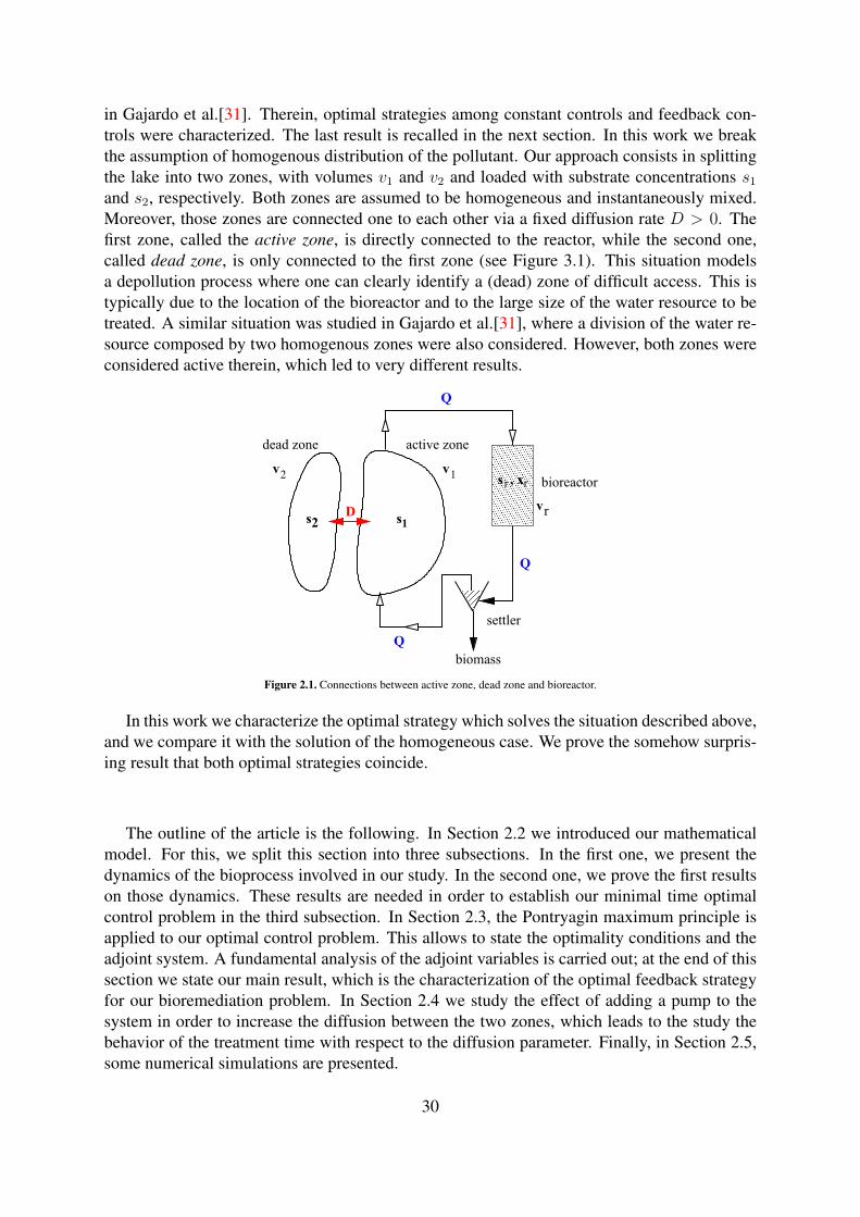
in Gajardo et al.[31]. Therein, optimal strategies among constant controls and feedback con-trols were characterized. The last result is recalled in the next section. In this work we breakthe assumption of homogenous distribution of the pollutant. Our approach consists in splittingthe lake into two zones, with volumes v1 and v2 and loaded with substrate concentrations s1

and s2, respectively. Both zones are assumed to be homogeneous and instantaneously mixed.Moreover, those zones are connected one to each other via a fixed diffusion rate D > 0. Thefirst zone, called the active zone, is directly connected to the reactor, while the second one,called dead zone, is only connected to the first zone (see Figure 3.1). This situation modelsa depollution process where one can clearly identify a (dead) zone of difficult access. This istypically due to the location of the bioreactor and to the large size of the water resource to betreated. A similar situation was studied in Gajardo et al.[31], where a division of the water re-source composed by two homogenous zones were also considered. However, both zones wereconsidered active therein, which led to very different results.

Q

s2 s1

1v

2v

rv

s , xrr bioreactor

biomass

settler

D

dead zone active zone

Q

Q

Figure 2.1. Connections between active zone, dead zone and bioreactor.

In this work we characterize the optimal strategy which solves the situation described above,and we compare it with the solution of the homogeneous case. We prove the somehow surpris-ing result that both optimal strategies coincide.

The outline of the article is the following. In Section 2.2 we introduced our mathematicalmodel. For this, we split this section into three subsections. In the first one, we present thedynamics of the bioprocess involved in our study. In the second one, we prove the first resultson those dynamics. These results are needed in order to establish our minimal time optimalcontrol problem in the third subsection. In Section 2.3, the Pontryagin maximum principle isapplied to our optimal control problem. This allows to state the optimality conditions and theadjoint system. A fundamental analysis of the adjoint variables is carried out; at the end of thissection we state our main result, which is the characterization of the optimal feedback strategyfor our bioremediation problem. In Section 2.4 we study the effect of adding a pump to thesystem in order to increase the diffusion between the two zones, which leads to the study thebehavior of the treatment time with respect to the diffusion parameter. Finally, in Section 2.5,some numerical simulations are presented.

30

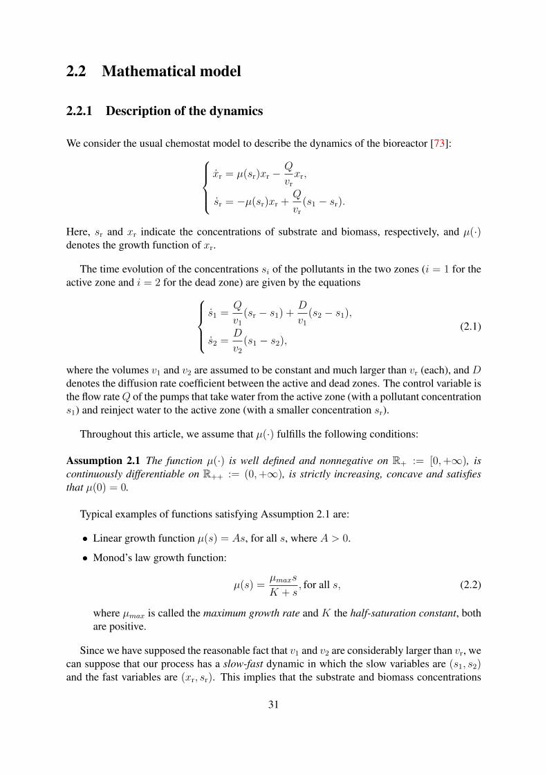
2.2 Mathematical model

2.2.1 Description of the dynamics

We consider the usual chemostat model to describe the dynamics of the bioreactor [73]:xr = µ(sr)xr −

Q

vr

xr,

sr = −µ(sr)xr +Q

vr

(s1 − sr).

Here, sr and xr indicate the concentrations of substrate and biomass, respectively, and µ(·)denotes the growth function of xr.

The time evolution of the concentrations si of the pollutants in the two zones (i = 1 for theactive zone and i = 2 for the dead zone) are given by the equations

s1 =Q

v1

(sr − s1) +D

v1

(s2 − s1),

s2 =D

v2

(s1 − s2),

(2.1)

where the volumes v1 and v2 are assumed to be constant and much larger than vr (each), and Ddenotes the diffusion rate coefficient between the active and dead zones. The control variable isthe flow rateQ of the pumps that take water from the active zone (with a pollutant concentrations1) and reinject water to the active zone (with a smaller concentration sr).

Throughout this article, we assume that µ(·) fulfills the following conditions:

Assumption 2.1 The function µ(·) is well defined and nonnegative on R+ := [0,+∞), iscontinuously differentiable on R++ := (0,+∞), is strictly increasing, concave and satisfiesthat µ(0) = 0.

Typical examples of functions satisfying Assumption 2.1 are:

• Linear growth function µ(s) = As, for all s, where A > 0.

• Monod’s law growth function:

µ(s) =µmaxs

K + s, for all s, (2.2)

where µmax is called the maximum growth rate and K the half-saturation constant, bothare positive.

Since we have supposed the reasonable fact that v1 and v2 are considerably larger than vr, wecan suppose that our process has a slow-fast dynamic in which the slow variables are (s1, s2)and the fast variables are (xr, sr). This implies that the substrate and biomass concentrations

31

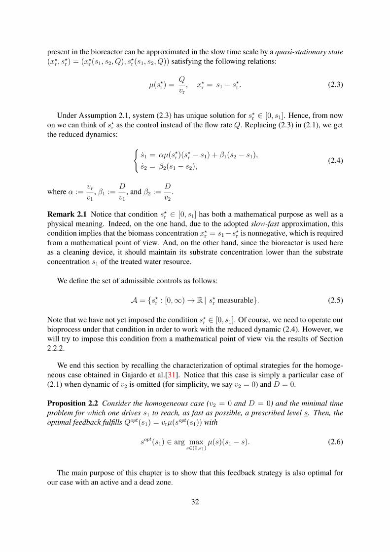
present in the bioreactor can be approximated in the slow time scale by a quasi-stationary state(x?r , s

?r ) = (x?r (s1, s2, Q), s?r (s1, s2, Q)) satisfying the following relations:

µ(s?r ) =Q

vr

, x?r = s1 − s?r . (2.3)

Under Assumption 2.1, system (2.3) has unique solution for s?r ∈ [0, s1]. Hence, from nowon we can think of s?r as the control instead of the flow rate Q. Replacing (2.3) in (2.1), we getthe reduced dynamics:

s1 = αµ(s?r )(s?r − s1) + β1(s2 − s1),

s2 = β2(s1 − s2),(2.4)

where α :=vr

v1

, β1 :=D

v1

, and β2 :=D

v2

.

Remark 2.1 Notice that condition s?r ∈ [0, s1] has both a mathematical purpose as well as aphysical meaning. Indeed, on the one hand, due to the adopted slow-fast approximation, thiscondition implies that the biomass concentration x?r = s1−s?r is nonnegative, which is requiredfrom a mathematical point of view. And, on the other hand, since the bioreactor is used hereas a cleaning device, it should maintain its substrate concentration lower than the substrateconcentration s1 of the treated water resource.

We define the set of admissible controls as follows:

A = s?r : [0,∞)→ R | s?r measurable. (2.5)

Note that we have not yet imposed the condition s?r ∈ [0, s1]. Of course, we need to operate ourbioprocess under that condition in order to work with the reduced dynamic (2.4). However, wewill try to impose this condition from a mathematical point of view via the results of Section2.2.2.

We end this section by recalling the characterization of optimal strategies for the homoge-neous case obtained in Gajardo et al.[31]. Notice that this case is simply a particular case of(2.1) when dynamic of v2 is omitted (for simplicity, we say v2 = 0) and D = 0.

Proposition 2.2 Consider the homogeneous case (v2 = 0 and D = 0) and the minimal timeproblem for which one drives s1 to reach, as fast as possible, a prescribed level s. Then, theoptimal feedback fulfills Qopt(s1) = vrµ(sopt(s1)) with

sopt(s1) ∈ arg maxs∈(0,s1)

µ(s)(s1 − s). (2.6)

The main purpose of this chapter is to show that this feedback strategy is also optimal forour case with an active and a dead zone.

32

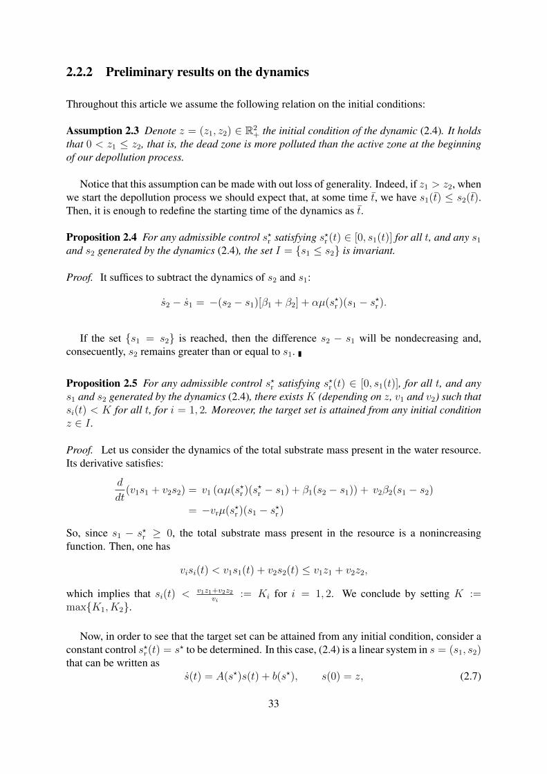
2.2.2 Preliminary results on the dynamics

Throughout this article we assume the following relation on the initial conditions:

Assumption 2.3 Denote z = (z1, z2) ∈ R2+ the initial condition of the dynamic (2.4). It holds

that 0 < z1 ≤ z2, that is, the dead zone is more polluted than the active zone at the beginningof our depollution process.

Notice that this assumption can be made with out loss of generality. Indeed, if z1 > z2, whenwe start the depollution process we should expect that, at some time t, we have s1(t) ≤ s2(t).Then, it is enough to redefine the starting time of the dynamics as t.

Proposition 2.4 For any admissible control s?r satisfying s?r (t) ∈ [0, s1(t)] for all t, and any s1

and s2 generated by the dynamics (2.4), the set I = s1 ≤ s2 is invariant.

Proof. It suffices to subtract the dynamics of s2 and s1:

s2 − s1 = −(s2 − s1)[β1 + β2] + αµ(s?r )(s1 − s?r ).

If the set s1 = s2 is reached, then the difference s2 − s1 will be nondecreasing and,consecuently, s2 remains greater than or equal to s1.

Proposition 2.5 For any admissible control s?r satisfying s?r (t) ∈ [0, s1(t)], for all t, and anys1 and s2 generated by the dynamics (2.4), there exists K (depending on z, v1 and v2) such thatsi(t) < K for all t, for i = 1, 2. Moreover, the target set is attained from any initial conditionz ∈ I .

Proof. Let us consider the dynamics of the total substrate mass present in the water resource.Its derivative satisfies:

d

dt(v1s1 + v2s2) = v1 (αµ(s?r )(s?r − s1) + β1(s2 − s1)) + v2β2(s1 − s2)

= −vrµ(s?r )(s1 − s?r )

So, since s1 − s?r ≥ 0, the total substrate mass present in the resource is a nonincreasingfunction. Then, one has

visi(t) < v1s1(t) + v2s2(t) ≤ v1z1 + v2z2,

which implies that si(t) < v1z1+v2z2vi

:= Ki for i = 1, 2. We conclude by setting K :=maxK1, K2.

Now, in order to see that the target set can be attained from any initial condition, consider aconstant control s?r(t) = s? to be determined. In this case, (2.4) is a linear system in s = (s1, s2)that can be written as

s(t) = A(s?)s(t) + b(s?), s(0) = z, (2.7)

33

where

A(s?) =

(−αµ(s?)− β1 β1

β2 −β2

), b(s?) =

(αµ(s?)s?

0.

)From the analysis of the trace and the determinant of the matrix A(s?), we conclude that

this is an invertible matrix with two different real negative eigenvalues. Then, the solution of(2.7) converges to the equilibrium point s∞ = −A(s?)−1b(s?) = (s?, s?), concluding that s2(t)converges to s? as t goes to infinity. We choose for the control the constant values s? = s/2 ifs1(0) ≥ s or s? ∈ (0, s1(0)) if s1(0) < s. Notice that the set I? := s2 ≥ s1 ≥ s? is positivelyinvariant. Indeed, for any t ≥ 0 such that s2(t) > s1(t) = s?, we have s1(t) > 0, and for anyt ≥ 0 such that s2(t) = s1(t) > s? we can apply Proposition 2.4. Thus, the control s?r (t) = s?

satisfies s?r (t) ∈ [0, s1(t)] for all t up to the final time, and there exists a finite time t† > 0 suchthat s2(t†) = s, concluding that this control leads the system to the target set in finite time.

2.2.3 Minimal time optimal control problem

In this section we describe our problem as a minimal time optimal control problem. For this,first note that, thanks to Assumption 2.3 and Proposition 2.4, to know the time of depollution itis enough to measure the dead zone pollutant’s concentration s2. Consequently, our target setcan be defined as

T = (s1, s2) ∈ R2+ | s2 ≤ s = R+ × [0, s]. (2.8)

On the other hand, due to Proposition 2.5, we expect to deal with admissible bounded con-trols. Since we are interested in controls s?r (·) ∈ A that satisfy s?r (t) ∈ [0, s1(t)] for all t ≥ 0,our admissible control set will be restricted to

AU := s?r ∈ A | s?r (t) ∈ [0, s1(t)], for all t ≥ 0.

Hence, in this work, we consider the following optimization problem:

(P) infs?r∈AU

T | s(0) = z, s(T ) ∈ T .

In what follows will show that the optimal solution s?r of (P) is given by a feedback controlthat coincides with the solution of the problem with the homogeneous zone.

We have the following proposition:

Proposition 2.6 For any initial condition z ∈ I there exists a unique solution for Problem (P).

Proof. The dynamics (2.4) are continuous with respect to (s, s?r ). Then, for fixed s ∈ R2+,

the velocity set generated as the image of the compact and connected set [0, s1] by dynamics(2.4) is a compact and connected set and, since the control variable s?r only acts in the firstcomponent, the velocity set is a segment and thus convex. This result, along with Propositions2.4 and 2.5, assure that hypotheses of Filippov’s theorem [17, Theorem 9.2.i] are satisfied, thusproving the existence of an optimal control for problem (P).

34

2.3 Application of Pontryagin maximum principle

The Hamiltonian of problem (P) is the mapping H : R2+ × R2 × R+ → R given by

H(s, λ; s?r ) = −1 + λ1αµ(s?r )(s?r − s1) + (−λ1β1 + λ2β2)(s1 − s2).

According to the Pontryagin maximum principle [19], if s?r (·) is a solution of (P) withcorresponding optimal trajectory s(·) = (s1(·), s2(·)), then there exists an adjoint state λ(·) =(λ1(·), λ2(·)), with no both components equal to zero at the same time, such that

λ1 = (αµ(s?r ) + β1)λ1 − β2λ2,

λ2 = −β1λ1 + β2λ2,(2.9)

and

H(s(t), λ(t); s?r (t)) = maxsr∈[0,s1(t)]

H(s(t), λ(t); sr). (2.10)

With these dynamics we can associate the transversality conditions

λ1(T ) = 0 and λ2(T ) < 0, (2.11)

where T denotes the optimal time (this notation is consistent with the definition of problem(P)).

Remark 2.2 It is possible to write the maximum principle even though the control set dependson the state s1(t), at each time instant t ≥ 0. Indeed, it suffices to do a change of variable u(t) ∈[0, 1] to have a control u(·) whose control set is compact and convex and whose associateds?r (t) = u(t)s1(t) is an admissible control, rewrite the dynamics accordingly, and restate themaximum principle. The result is equivalent to our approach.

Condition (2.10) states that, for a fixed time t, s?r (t) maximizes the function

φ(t, s?r ) = −λ1(t)µ(s?r )(s1(t)− s?r ), (2.12)

Concerning the behavior of the adjoint state λ1(·), we have the following proposition.

Proposition 2.7 The adjoint state λ(·) associated with an optimal solution of problem (P)satisfies that λ1(t) < 0 for all t ∈ [0, T ).

Proof. If one writes the adjoint equations (2.9) as λi = φi(t, λ1, λ2) (i = 1, 2), one can noticethat the partial derivatives ∂jφi (i 6= j) are non-positive. From the theory of monotone dynam-ical systems (see for instance [74]), the dynamics (2.9) are thus competitive or, equivalently,cooperative in backward time. As the transversality conditions (2.11) give λi(T ) ≤ 0 (i = 1, 2),we deduce by the property of monotone dynamics that one should have λi(t) ≤ 0 (i = 1, 2) forany t ≤ T . Now, if there exists t < T such that λ1(t) = 0, then one should have λ2(t) < 0.This implies λ1(t) > 0 (because β1 > 0), thus obtaining that the trajectory never returns to thethird quadrant, leading to a contradiction with the trasversality condition λ1(T ) = 0.

35

Let us define, for s1 > 0, the value s?r = s?r (s1) as the solution s?r in (0, s1) of the problem

s?r (s1) := arg maxs?r∈(0,s1)

µ(s?r )(s1 − s?r ), (2.13)

that is given by the unique solution of the equation

µ(s?r ) = µ′(s?r )(s1 − s?r ). (2.14)

For each s1 > 0 the solution of is unique. Indeed, if we define β(s1, s?r ) := µ(s?r )(s1 − s?r ),

thanks to Assumption 2.1, for fixed s1 > 0 the function s?r 7→ β(s1, s?r ) is positive in the interval

(0, s1), β(s1, 0) = β(s1, s1) = 0, and its second derivative is strictly negative, concluding thatit is strictly concave in (0, s1).

We also define the function

γ(s1) := maxs?r∈(0,s1)

µ(s?r )(s1 − s?r ) = µ(s?r (s1))(s1 − s?r (s1)). (2.15)

We are now in position to establish the main result of our article.

Proposition 2.8 The optimal flow rate Q?, which solves the depollution problem stated inSection 1, is given by Q?(s1) = vrµ(s?r (s1)), where s?r (·) is the unique solution of the optimalcontrol problem (P). This solution is characterized by the feedback control defined in (2.3). Inparticular, the optimal feedback control s?r satisfies that s?r ∈ [0, s1(t)], for all t ∈ [0, T ].

Proof. Let φ be the function defined in (2.12). Since λ1(t) < 0, for all t ∈ [0, T ) (byProposition 2.7), we notice s?r (t) maximizes the Hamiltonian with respect to sr, or equivalently,maximizes ψ(t, sr) = µ(sr)(s1(t) − sr) with respect to sr on [0, s1(t)]. Then, s?r has to havethe form s?r (t) = s?r (s1(t)), or equivalently, s?r is characterized by the feedback rule (2.3).Moreover, at its maximum with respect to s?r , ψ satisfies Fermat’s theorem on minima andmaxima: ∂

∂s?rψ(t, s?r ) = 0, which exactly coincides with (2.14).

Remark 2.3 Proposition 2.8 shows us that the optimal feedback policy does not depend on s2.However, the optimal time does.

Remark 2.4 In Remark 2.2 it was mentioned that the change of control s?r (t) = u(t)s1(t)allows to deal with controls u(·) whose set is independent of the state variable s1. The completeexpression of the adjoint equations is

λ1 = (αµ(us1) + β1)λ1 − β2λ2 + λ1αu(µ′(us1)s1(1− u)− µ(us1)),

λ2 = −β1λ1 + β2λ2,(2.16)

These equations, along with the maximum principle, allow to prove that the adjoint state λ1 isstrictly negative in the whole interval [0, T ) in the same manner than in Proposition 2.7 and, inparticular, to conclude the equality (µ′(u(t)s1(t))s1(t)(1− u(t))− µ(u(t)s1(t))) = 0 along anoptimal pair (s(·), u(·)). For the sake of interpretation of the variables, we continued workingwith s?r instead of u.

36

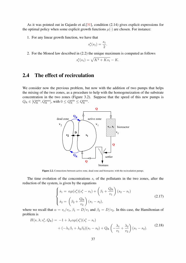
As it was pointed out in Gajardo et al.[31], condition (2.14) gives explicit expressions forthe optimal policy when some explicit growth functions µ(·) are chosen. For instance:

1. For any linear growth function, we have that

s?r (s1) =s1

2.

2. For the Monod law described in (2.2) the unique maximum is computed as follows

s?r (s1) =√K2 +Ks1 −K.

2.4 The effect of recirculation

We consider now the previous problem, but now with the addition of two pumps that helpsthe mixing of the two zones, as a procedure to help with the homogeneization of the substrateconcentration in the two zones (Figure 3.2). Suppose that the speed of this new pumps isQR ∈ [Qmin

R , QmaxR ], with 0 ≤ Qmin

R ≤ QmaxR .

Q

s2 s1

1v

2v

rv

s , xrr bioreactor

biomass

settler

dead zone active zone

Q

Q

QR

QR

D

Figure 2.2. Connections between active zone, dead zone and bioreactor, with the recirculation pumps.

The time evolution of the concentrations si of the pollutants in the two zones, after thereduction of the system, is given by the equations

s1 = αµ(s?r )(s?r − s1) +

(β1 +

QR

v1

)(s2 − s1)

s2 =

(β2 +

QR

v2

)(s1 − s2),

(2.17)

where we recall that α = vr/v1, β1 = D/v1 and β2 = D/v2. In this case, the Hamiltonian ofproblem is

H(s, λ; s?r , QR) = −1 + λ1αµ(s?r )(s?r − s1)

+ (−λ1β1 + λ2β2)(s1 − s2) +QR

(−λ1

v1

+λ2

v2

)(s1 − s2).

(2.18)

37

We say that a control (s?r , QR) is admissible if it satisfies for all t ≥ 0 that s?r (t) ∈ [0, s1(t)]and QR(t) ∈ [Qmin

R , QmaxR ]. We consider the same problem of minimum-time depollution.

Propositions 2.4 and 2.5 are still valid. The maximum principle states that if (s?r , QR) is asolution of the problem, then there exist an adjoint state λ(·) non-null at every time that solvesthe adjoint equations and transversality conditions

λ1 = αµ(s?r )λ1 − (D +QR)

(−λ1

v1

+λ2

v2

), λ1(T ) = 0,

λ2 = (D +QR)

(−λ1

v1

+λ2

v2

), λ2(T ) < 0,

(2.19)

and such that for each time t ∈ [0, T ] the Hamiltonian is maximized at the control value(s?r , QR(t)). Notice that this is equivalent to the independent maximization of the functionsφ(t, sr) with respect to sr ∈ [0, s1(t)] and of the function

QR 7→ QR

(−λ1

v1

+λ2

v2

)(s1 − s2).

Proposition 2.9 Suppose that (s?r , QR) is an optimal control for the problem with recirculation.Then, for all t ∈ [0, T ], the control s?r is given by the feedback control defined in (2.3), and wehave that QR(t) = Qmax

R .

Proof. The proof that s?r (t) = s?r (s1(t)) is the same as in Proposition 2.8; it relies in the factsthat the Hamiltonian is decoupled in the variables s?r and QR, and in the nonpositivity of theadjoint state λ1, whose proof is the same as in Proposition 2.7.

Let us define the function

η(t) =λ1(t)

v1

− λ2(t)

v2

. (2.20)

Notice that the maximimization of the Hamiltonian along the optimal trajectory and the invari-ance of the set I implies that QR(t) maximizes the function QR 7→ QRη(t), for all t ∈ [0, T ].We have that the time derivative of η(·) is

η = λ1α1

v1

µ(s?r ) + (D +QR)

(1

v1

+1

v2

)η,

with final value η(T ) = −λ2(T )/v1 > 0. We prove that this function is positive for all t ∈[0, T ). Suppose that for some time t† < T we have η(t†) = 0. Then, we have that η(t†) =α1µ(s?r (t†))λ1(t†) < 0, and thus η(t) ≤ 0 for all t ∈ [t†, T ]. This contradicts the fact that at thefinal time η(T ) > 0, concluding the statement.

Since η is positive along the optimal trajectory, then for all t ∈ [0, T ] the control value thatmaximizes QR 7→ QRη(t) is QR = Qmax

R .

This last result states that if it is possible to add a recirculation to the process, it is better touse the maximum speed of pumping during all the process. It seems natural to eliminateQR as a

38

control parameter (since it will not change along the optimal trajectory), and to consider insteadits maximum value Qmax

R as a modification of the diffusion term. We can rename D + QmaxR

simply as D (and, in consequence, return to the system (2.4)), and to study the behavior of theminimal-time function with respect to this parameter. It seems natural to ask if the best possiblescenario is the homogeneous one, that is, the case with infinite diffusion.

Let us denote the minimal-time function by VD(·), indexed by the value of the diffusionparameter D:

VD(z) = infs?r∈AU

T ≥ 0 | sz,s?r ,D(T ) ∈ T ,

where sz,s?r ,D(·) denotes the solution of with initial condition z = (z1, z2) ∈ I and admissiblecontrol s?r . We have the following result.

Proposition 2.10 For any z ∈ I , the function D 7→ VD(z) is decreasing.

Proof. From Proposition 2.8, we know that for every D > 0 and initial condition z ∈ I , theoptimal control s?r (·) is given by s?r (t) = s?r (s

z,s?r ,D1 (t)) with s?r (·) the feedback given in (2.3)

and sz,s?r ,D(·) the solution of (2.4) with initial condition z and control s?r . We split the proof intwo parts:

i. Notice that under the optimal feedback, sz,s?r ,D

2 (·) is decreasing; thus, we can define thetime change

τ(t) = z2 − sz,s?r ,D

2 (t).

The time τ ranges from 0 to τf := z2 − s (independent of D); from (2.4) we get theformula for the final time (depending on D)

T = TD =v2

D

∫ τf

0

dτ

s2(τ,D)− s1(τ,D).

Now, s1(·) is solution of the nonautonomous equation in time τ

d

dτs1 = fD(τ, s1) := −αv2

D

γ(s1)

z2 − τ − s1

+v2

v1

. (2.21)

Notice that for D1 < D2 we have fD1(τ, s1) < fD2(τ, s1), which implies that for allτ ∈ [0, τf ], s1(τ,D1) < s1(τ,D2). We conclude that sz,s

?r ,D

1 (T ) is increasing with D.

ii. Now, the variable m(t) = v1sz,s?r ,D1 (t) + v2s

z,s?r ,D2 (t) is also decreasing in time, with

m(t) = −vrγ(sz,s?r ,D1 (t)). We define the time change

θ(t) = m0 −m(t), m0 = v1z1 + v2z2,

which ranges from θ = 0 to θDf := m0 − (v1sz,s?r ,D1 (T ) + v2s). From the point i. we see

that θDf is decreasing with D. Again, from (2.4), we obtain an expression for the finaltime:

TD =1

vr

∫ θDf

0

dθ

γ(s1(θ,D)). (2.22)

39

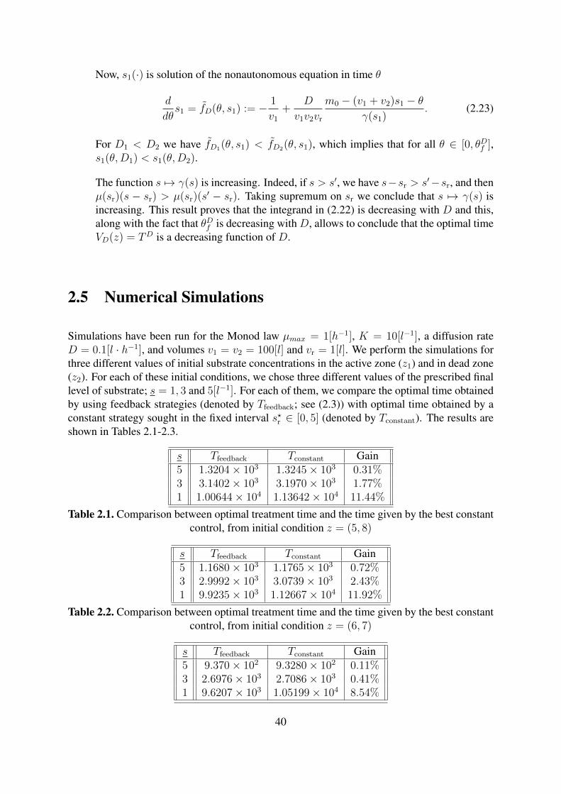
Now, s1(·) is solution of the nonautonomous equation in time θ

d

dθs1 = fD(θ, s1) := − 1

v1

+D

v1v2vr

m0 − (v1 + v2)s1 − θγ(s1)

. (2.23)

For D1 < D2 we have fD1(θ, s1) < fD2(θ, s1), which implies that for all θ ∈ [0, θDf ],s1(θ,D1) < s1(θ,D2).

The function s 7→ γ(s) is increasing. Indeed, if s > s′, we have s−sr > s′−sr, and thenµ(sr)(s − sr) > µ(sr)(s

′ − sr). Taking supremum on sr we conclude that s 7→ γ(s) isincreasing. This result proves that the integrand in (2.22) is decreasing with D and this,along with the fact that θDf is decreasing with D, allows to conclude that the optimal timeVD(z) = TD is a decreasing function of D.

2.5 Numerical Simulations

Simulations have been run for the Monod law µmax = 1[h−1], K = 10[l−1], a diffusion rateD = 0.1[l · h−1], and volumes v1 = v2 = 100[l] and vr = 1[l]. We perform the simulations forthree different values of initial substrate concentrations in the active zone (z1) and in dead zone(z2). For each of these initial conditions, we chose three different values of the prescribed finallevel of substrate; s = 1, 3 and 5[l−1]. For each of them, we compare the optimal time obtainedby using feedback strategies (denoted by Tfeedback; see (2.3)) with optimal time obtained by aconstant strategy sought in the fixed interval s?r ∈ [0, 5] (denoted by Tconstant). The results areshown in Tables 2.1-2.3.

s Tfeedback Tconstant Gain5 1.3204× 103 1.3245× 103 0.31%3 3.1402× 103 3.1970× 103 1.77%1 1.00644× 104 1.13642× 104 11.44%

Table 2.1. Comparison between optimal treatment time and the time given by the best constantcontrol, from initial condition z = (5, 8)

s Tfeedback Tconstant Gain5 1.1680× 103 1.1765× 103 0.72%3 2.9992× 103 3.0739× 103 2.43%1 9.9235× 103 1.12667× 104 11.92%

Table 2.2. Comparison between optimal treatment time and the time given by the best constantcontrol, from initial condition z = (6, 7)

s Tfeedback Tconstant Gain5 9.370× 102 9.3280× 102 0.11%3 2.6976× 103 2.7086× 103 0.41%1 9.6207× 103 1.05199× 104 8.54%

40

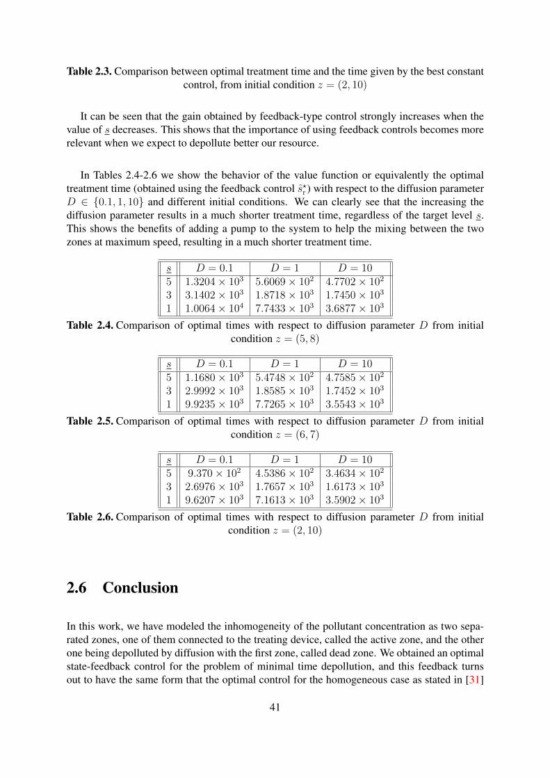
Table 2.3. Comparison between optimal treatment time and the time given by the best constantcontrol, from initial condition z = (2, 10)

It can be seen that the gain obtained by feedback-type control strongly increases when thevalue of s decreases. This shows that the importance of using feedback controls becomes morerelevant when we expect to depollute better our resource.

In Tables 2.4-2.6 we show the behavior of the value function or equivalently the optimaltreatment time (obtained using the feedback control s?r ) with respect to the diffusion parameterD ∈ 0.1, 1, 10 and different initial conditions. We can clearly see that the increasing thediffusion parameter results in a much shorter treatment time, regardless of the target level s.This shows the benefits of adding a pump to the system to help the mixing between the twozones at maximum speed, resulting in a much shorter treatment time.

s D = 0.1 D = 1 D = 105 1.3204× 103 5.6069× 102 4.7702× 102

3 3.1402× 103 1.8718× 103 1.7450× 103

1 1.0064× 104 7.7433× 103 3.6877× 103

Table 2.4. Comparison of optimal times with respect to diffusion parameter D from initialcondition z = (5, 8)

s D = 0.1 D = 1 D = 105 1.1680× 103 5.4748× 102 4.7585× 102

3 2.9992× 103 1.8585× 103 1.7452× 103

1 9.9235× 103 7.7265× 103 3.5543× 103

Table 2.5. Comparison of optimal times with respect to diffusion parameter D from initialcondition z = (6, 7)

s D = 0.1 D = 1 D = 105 9.370× 102 4.5386× 102 3.4634× 102

3 2.6976× 103 1.7657× 103 1.6173× 103

1 9.6207× 103 7.1613× 103 3.5902× 103

Table 2.6. Comparison of optimal times with respect to diffusion parameter D from initialcondition z = (2, 10)

2.6 Conclusion

In this work, we have modeled the inhomogeneity of the pollutant concentration as two sepa-rated zones, one of them connected to the treating device, called the active zone, and the otherone being depolluted by diffusion with the first zone, called dead zone. We obtained an optimalstate-feedback control for the problem of minimal time depollution, and this feedback turnsout to have the same form that the optimal control for the homogeneous case as stated in [31]

41

where there is no dead zone, depending only of the measurements on the active zone. This hassome interesting features for practitioners, for instance it does not require the knowledge of thevolumes of the two zones or the diffusion parameter.

We have also shown that the optimal treatment time is decreasing with the diffusion param-eter. We show this behavior by means of numerical simulations.

42

Chapter 3

Optimal feedback synthesis and minimaltime function for the bioremediation ofwater resources with two patches

This chapter corresponds to the published article

Ramírez C., H.; Rapaport, A.; Riquelme, V. Optimal Feedback Synthesis and Minimal TimeFunction for the Bioremediation of Water Resources with Two Patches. SIAM J. Control

Optim. 54 (2016), no. 3, 1697-1718.

3.1 Introduction

Today, the decontamination of water resources and reservoirs in natural environments (lakes,lagoons, etc.) and in industrial frameworks (basin, pools, etc.) is of prime importance. Dueto the availability of drinking water becoming scarce on earth, efforts have to be made to re-use water and to preserve aquatic resources. To this end, biological treatment is a convenientway to extract organic or soluble matter from water. The basic principle is to use biotic agents(generally micro-organisms) that convert the pollutant until the concentration in the reservoirdecreases to an acceptable level. Typically, the treatment is performed with the help of con-tinuously stirred or fed-batch bioreactors. Numerous studies have been devoted to this subjectover the past 40 years (see, for instance, [3, 22, 23, 32, 42, 43, 50, 60, 71, 72, 76, 78]).

The following main types of procedure are usually considered:

• The direct introduction of the biotic agents to the reservoir. This solution could lead tothe eutrophication of the resource.

• The draining of the reservoir to a dedicated bioreactor and the filling back of the waterafter treatment. This solution attempts to eradicate various forms of life supported by thewater resource, that cannot survive without water (such as fish, algae, etc.).

43

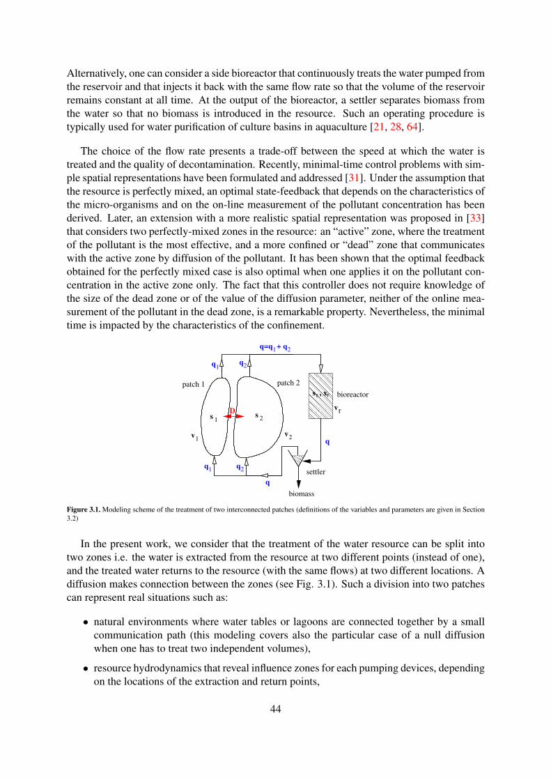
Alternatively, one can consider a side bioreactor that continuously treats the water pumped fromthe reservoir and that injects it back with the same flow rate so that the volume of the reservoirremains constant at all time. At the output of the bioreactor, a settler separates biomass fromthe water so that no biomass is introduced in the resource. Such an operating procedure istypically used for water purification of culture basins in aquaculture [21, 28, 64].

The choice of the flow rate presents a trade-off between the speed at which the water istreated and the quality of decontamination. Recently, minimal-time control problems with sim-ple spatial representations have been formulated and addressed [31]. Under the assumption thatthe resource is perfectly mixed, an optimal state-feedback that depends on the characteristics ofthe micro-organisms and on the on-line measurement of the pollutant concentration has beenderived. Later, an extension with a more realistic spatial representation was proposed in [33]that considers two perfectly-mixed zones in the resource: an “active” zone, where the treatmentof the pollutant is the most effective, and a more confined or “dead” zone that communicateswith the active zone by diffusion of the pollutant. It has been shown that the optimal feedbackobtained for the perfectly mixed case is also optimal when one applies it on the pollutant con-centration in the active zone only. The fact that this controller does not require knowledge ofthe size of the dead zone or of the value of the diffusion parameter, neither of the online mea-surement of the pollutant in the dead zone, is a remarkable property. Nevertheless, the minimaltime is impacted by the characteristics of the confinement.

q1

q2

q=q + q1 2

1s 2s

2vv

1

rv

s , xrr bioreactor

biomass

settler

q

patch 2patch 1

q1

q2

q

D

Figure 3.1. Modeling scheme of the treatment of two interconnected patches (definitions of the variables and parameters are given in Section3.2)

In the present work, we consider that the treatment of the water resource can be split intotwo zones i.e. the water is extracted from the resource at two different points (instead of one),and the treated water returns to the resource (with the same flows) at two different locations. Adiffusion makes connection between the zones (see Fig. 3.1). Such a division into two patchescan represent real situations such as:

• natural environments where water tables or lagoons are connected together by a smallcommunication path (this modeling covers also the particular case of a null diffusionwhen one has to treat two independent volumes),

• resource hydrodynamics that reveal influence zones for each pumping devices, dependingon the locations of the extraction and return points,

44

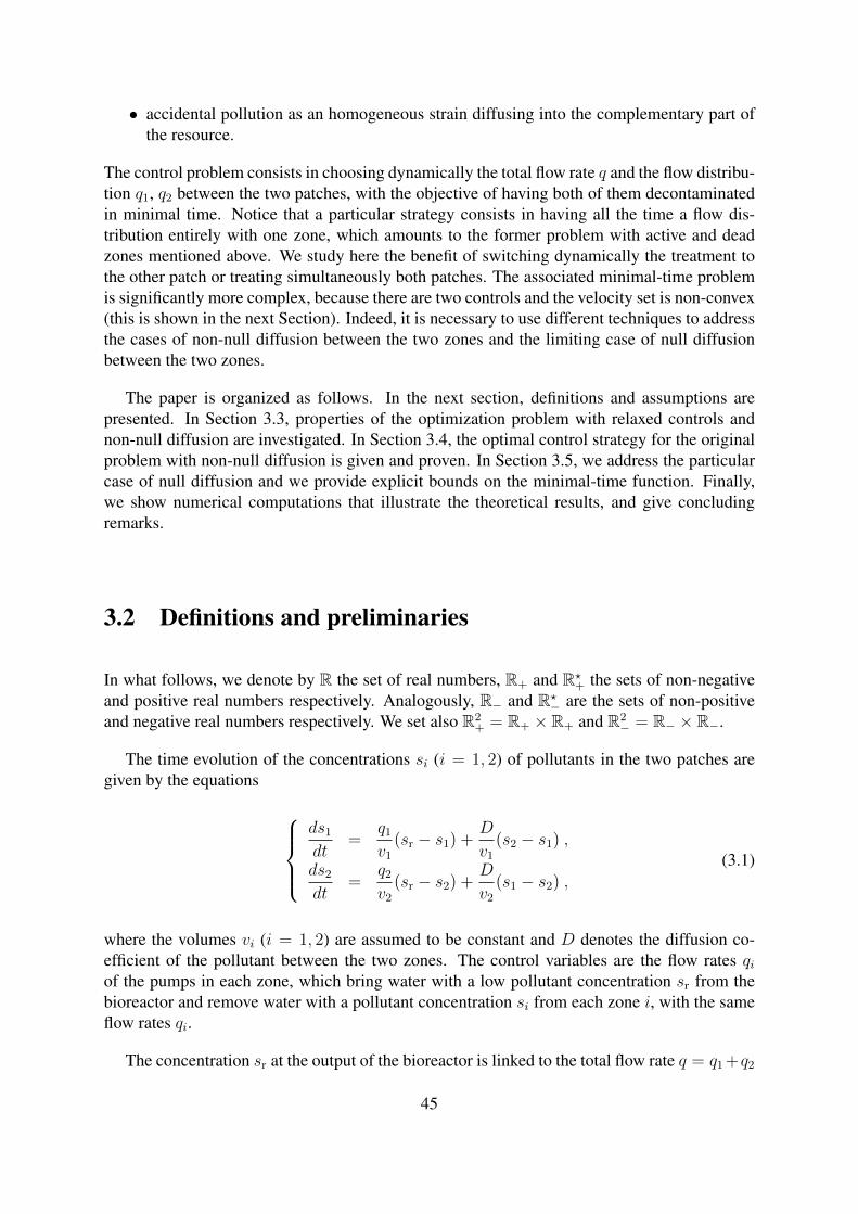
• accidental pollution as an homogeneous strain diffusing into the complementary part ofthe resource.

The control problem consists in choosing dynamically the total flow rate q and the flow distribu-tion q1, q2 between the two patches, with the objective of having both of them decontaminatedin minimal time. Notice that a particular strategy consists in having all the time a flow dis-tribution entirely with one zone, which amounts to the former problem with active and deadzones mentioned above. We study here the benefit of switching dynamically the treatment tothe other patch or treating simultaneously both patches. The associated minimal-time problemis significantly more complex, because there are two controls and the velocity set is non-convex(this is shown in the next Section). Indeed, it is necessary to use different techniques to addressthe cases of non-null diffusion between the two zones and the limiting case of null diffusionbetween the two zones.

The paper is organized as follows. In the next section, definitions and assumptions arepresented. In Section 3.3, properties of the optimization problem with relaxed controls andnon-null diffusion are investigated. In Section 3.4, the optimal control strategy for the originalproblem with non-null diffusion is given and proven. In Section 3.5, we address the particularcase of null diffusion and we provide explicit bounds on the minimal-time function. Finally,we show numerical computations that illustrate the theoretical results, and give concludingremarks.

3.2 Definitions and preliminaries

In what follows, we denote by R the set of real numbers, R+ and R?+ the sets of non-negative

and positive real numbers respectively. Analogously, R− and R?− are the sets of non-positive

and negative real numbers respectively. We set also R2+ = R+ × R+ and R2

− = R− × R−.

The time evolution of the concentrations si (i = 1, 2) of pollutants in the two patches aregiven by the equations

ds1

dt=

q1

v1

(sr − s1) +D

v1

(s2 − s1) ,

ds2

dt=

q2

v2

(sr − s2) +D

v2

(s1 − s2) ,(3.1)

where the volumes vi (i = 1, 2) are assumed to be constant and D denotes the diffusion co-efficient of the pollutant between the two zones. The control variables are the flow rates qiof the pumps in each zone, which bring water with a low pollutant concentration sr from thebioreactor and remove water with a pollutant concentration si from each zone i, with the sameflow rates qi.

The concentration sr at the output of the bioreactor is linked to the total flow rate q = q1 +q2

45

by the usual chemostat model:dsr

dt= −µ(sr)xr +

q

vr

(sin − sr) ,

dxr

dt= µ(sr)xr −

q

vr

xr ,(3.2)

where xr is the biomass concentration, vr is the volume of the bioreactor and µ(·) is the specificgrowth rate of the bacteria (without a loss of generality we assume that the yield coefficientis equal to one). These equations describe the dynamics of a bacterial growth consuming asubstrate that is constantly fed in a tank of constant volume (see for instance [73]). The inputconcentration sin is given here by the combination of the concentrations of the water extractedfrom the two zones:

sin =q1s1 + q2s2

q1 + q2

. (3.3)

We assume that the output of the bioreactor is filtered by a settler, that we assume to be perfect,so that the water that returns to the resource is biomass free (see [24, 25] for considerationsof settler modeling and conditions that ensure the stability of the desired steady-state of thesettler).

The target to be reached in the minimal time is defined by a threshold s > 0 of the pollutantconcentrations, that is

T =s = (s1, s2) ∈ R2

+ |maxs1, s2 ≤ s. (3.4)

In the paper, we shall denote tf as the first time at which a trajectory reaches the target (whenit exists).

We make the usual assumptions on the growth function µ(·) in absence of inhibition.

Assumption 3.1 µ(·) is a C1 increasing concave function defined on R+ with µ(0) = 0.

Under this last assumption, we recall that under a constant sin, the dynamics (3.2) admit aunique positive equilibrium (s?r , x

?r ) that is globally asymptotically stable on the domain R+ ×

R?+ provided that the condition q/vr ≤ µ(sin) is satisfied (see, for instance, [73]). Then, s?r is

defined as the unique solution of µ(s?r ) = q/vr and x?r = sin − s?r . Consequently, consideringexpression (3.3), the controls q1 and q2 are chosen such that

q1 + q2 ≤ vrµ

(q1s1 + q2s2

q1 + q2

). (3.5)

We assume that the resource to be treated is very large. This amounts to considering that thebioreactor is small compared to both zones of the resource.

Assumption 3.2 v1 and v2 are large compared to vr.

46

Let us define α = q1/q, r = v1/(v1 + v2), d = D/vr, and ε = vr/(v1 + v2). Then, thecoupled dynamics (3.1)-(3.2) with (3.3) can be written in the slow-fast form

dsr

dt= −µ(sr)xr +

q

vr

(αs1 + (1− α)s2 − sr) ,

dxr

dt= µ(sr)xr −

q

vr

xr ,

ds1

dt= ε

(α

r

q

vr

(sr − s1) +d

r(s2 − s1)

),

ds2

dt= ε

(1− α1− r

q

vr

(sr − s2) +d

1− r(s1 − s2)

).

(3.6)

Provided that the initial conditions of the variables (sr, xr) belong to R+ × R?+, applying Ty-

chonnof’s Theorem (see for instance [49]), the dynamics of the slow variables (s1, s2) can beapproached using the reduced dynamics

s1 =ds1

dτ=

α

rµ(s?r )(s?r − s1) +

d

r(s2 − s1) ,

s2 =ds2

dτ=

1− α1− r

µ(s?r )(s?r − s2) +d

1− r(s1 − s2)

(3.7)

in the time scale τ = εt. In this formulation, the quasi-steady-state concentration s?r of thebioreactor can be considered as a control variable that takes values in [0, αs1+(1−α)s2], whichis equivalent to choosing q ∈ [0, vrµ(αs1 +(1−α)s2)] when Assumption 3.1 is satisfied. In thefollowing, we shall consider the optimal control for the reduced dynamics only. Nevertheless,we give some properties of the optimal feedback for the reduced dynamics when applied to theun-reduced one, in Section 3.4 (Remark 3.2) and Appendix.

Notice that the control problem can be reformulated with the controls u = (α, s?r ) thatbelong to the state-dependent control set

U(s) = (α, s?r ) |α ∈ [0, 1], s?r ∈ [0, αs1 + (1− α)s2] (3.8)

equivalently to controls q1 and q2. In what follows, a measurable function u(·) such that u(t) ∈U(s(t)) for all t is called an admissible control.

Lemma 3.3 The domain R2+ is positively invariant by the dynamics (3.7) for any admissible

controls u(·), and any trajectory is bounded. Furthermore, the target T is reachable in a finitetime from any initial condition in R2

+.

Proof. For s1 = 0 and s2 ≥ 0, one has s1 ≥ 0. Similarly, one has s2 ≥ 0 when s1 ≥ 0 ands2 = 0. By the uniqueness of the solutions of (3.7) for measurable controls u(·), we deducethat R2

+ is invariant. From equations (3.7), one can write

rs1 + (1− r)s2 = µ(s?r )(s?r − (αs1 + (1− α)s2)) ≤ 0

for any admissible controls. One then deduces

rs1(t) + (1− r)s2(t) ≤M0 = rs1(0) + (1− r)s2(0), ∀t ≥ 0,

47

which provides the boundedness of the trajectories.

Consider the feedback strategy

α = r , s?r =rs1 + (1− r)s2

2,

and we write the dynamics of m = rs1 + (1− r)s2 as follows:

m = −µ(m

2

) m2< 0 ,∀m > 0 .

Then, from any initial condition in R2+, the solution m(t) tends to 0 when t tends to infinity.

Therefore, m(·) reaches the set [0,min(r, 1 − r)s] in a finite time, which guarantees that s =(s1, s2) belongs to T at that time.

For simplicity, we define the function

β(σ, s?r ) = µ(s?r )(σ − s?r ) (3.9)

so that the dynamics (3.7) can be written in the more compact form

s = F (s, u) + dG(s) (3.10)

where F (·) and G(·) are defined as follows:

F (s, (α, s?r )) = −

α

rβ(s1, s

?r )

1− α1− r

β(s2, s?r )

, G(s) =

s2 − s1

rs1 − s2

1− r

.

The dynamics can be equivalently expressed in terms of controls v = (α, ζ) that belong to thestate-independent set V = [0, 1]2 with the dynamics

s = F (s, (α, ζ(αs1 + (1− α)s2))) + dG(s) (3.11)

which satisfy the usual regularity conditions for applying Pontryagin’s Maximum Principle forderiving necessary optimality conditions. One can notice that the velocity set of the dynamics(3.11) is not everywhere convex. Consequently, one cannot guarantee a priori the existence ofan optimal control v(·) in the set of time-measurable functions that take values in V but thatare among relaxed controls (see, for instance, [83, Sec. 2.7]). For convenience, we shall keepthe formulation of the problem with controls u. Because for any s the sets ∪u∈U(s)F (s, u) aretwo-dimensional connected, the corresponding convexified dynamics can be written as follows(see [68, Th. 2.29]):

s = F (s, u) + dG(s) (3.12)

withF (s, u) = pF (s, ua) + (1− p)F (s, ub) (3.13)

48

where the relaxed controls u = (ua, ub, p) = (αa, s?ra, αb, s

?rb, p) belong to the set

U(s) = U(s)2 × [0, 1].

Thanks to Lemma 3.3, the hypotheses of Filippov’s existence theorem [17, Theorem 9.2.i]are satisfied for the relaxed dynamics (that is, with relaxed controls) and thus, for any initialcondition there exists a solution of the relaxed problem. In the next section, we show that therelaxed problem admits an optimal solution that is also a solution of the original (non-relaxed)problem.

3.3 Study of the relaxed problem

Throughout this section, we assume that the parameter d is positive. The particular case ofd = 0 will be considered later in Section 3.5. Let us write the Hamiltonian of the relaxedproblem

H(s, λ, (αa, s?ra, αb, s

?rb, p)) =

− 1 + pQ(s, λ, (αa, s?ra)) + (1− p)Q(s, λ, (αb, s

?rb)) + d(s2 − s1)

(λ1

r− λ2

1− r

)(3.14)

which is to be maximized w.r.t. (αa, s?ra, αb, s

?rb, p) ∈ U(s), where λ = (λ1, λ2), and we have

defined, for convenience, the function

Q(s, λ, (α, s?r )) = −(αλ1

rβ(s1, s

?r ) + (1− α)

λ2

1− rβ(s2, s

?r )

). (3.15)

The adjoint equations areλ1 = λ1

(pαarµ(s?ra) + (1− p)αb

rµ(s?rb) +

d

r

)− λ2

d

1− r,

λ2 = −λ1d

r+ λ2

(p

1− αa1− r

µ(s?ra) + (1− p)1− αb1− r

µ(s?rb) +d

1− r

),

(3.16)

with the following transversality conditionss1(tf ) < s, s2(tf ) = s ⇒ λ1(tf ) = 0, λ2(tf ) < 0 ,s1(tf ) = s, s2(tf ) < s ⇒ λ1(tf ) < 0, λ2(tf ) = 0 ,s1(tf ) = s, s2(tf ) = s ⇒ λ1(tf ) ≤ 0, λ2(tf ) ≤ 0 with λ(tf ) 6= 0 .

(3.17)

As usual, a triple (s(·), λ(·), u?(·)) satisfying (3.12), (3.16), (4.7), and

H(s(t), λ(t), u?(t)) = maxu∈U(s(t))

H(s(t), λ(t), u) (3.18)

is called an admissible extremal.

49

Lemma 3.4 Along any admissible extremal, one has λi(t) < 0 (i = 1, 2) for any t < tf .

Proof. If one writes the adjoint equations (3.16) as λi = φi(t, λ1, λ2) (i = 1, 2), one can noticethat the partial derivatives ∂jφi (i 6= j) are non-positive. From the theory of monotone dynam-ical systems (see for instance [74]), the dynamics (3.16) are thus competitive or, equivalently,cooperative in backward time. As the transversality conditions (4.7) gives λi(tf ) ≤ 0 (i = 1, 2),we deduce by the property of monotone dynamics that one should have λi(t) ≤ 0 (i = 1, 2) forany t ≤ tf . Moreover, λ = 0 is an equilibrium of (3.16) and λ(tf ) has to be different from 0 atany time t ≤ tf . Then, λi(t) (i = 1, 2) cannot be simultaneously equal to zero. If there existst < tf and i ∈ 1, 2 such that λi(t) = 0, then one should have λj(t) < 0 for j 6= i. However,d > 0 implies λi(t) > 0, thus obtaining a contradiction with λi ≤ 0 for any time from t to thefinal time tf .

For the following, we consider the function

γ(σ) = maxs?r≥0

β(σ, s?r ), σ > 0 , (3.19)

which satisfies the following property:

Lemma 3.5 Under Assumption 3.1, for any σ > 0, there exists a unique s?r (σ) ∈ (0, σ) thatrealizes the maximum in (3.19). Furthermore, the function γ(·) is differentiable and increasingwith

γ′(σ) = µ(s?r (σ)) . (3.20)

Proof. Consider the function ϕ : (σ,w) ∈ R+ × [0, 1] 7→ β(σ,wσ) and the partial functionϕσ : w ∈ [0, 1] 7→ ϕ(σ,w) for fixed σ > 0. Notice that ϕσ(0) = ϕσ(1) = 0 and that ϕσ(w) > 0for w ∈ (0, 1). Simple calculation gives ϕ′′σ(w) = µ′′(wσ)(1 − w)σ3 − 2µ′(wσ)σ2, which isnegative. Therefore, ϕσ(·) is a strictly concave function on [0, 1] and consequently admits aunique maximum w?σ on [0, 1]. We conclude that w?σ belongs to (0, 1) or, equivalently, that themaximum of s?r 7→ β(σ, s?r ) is realized for a unique s?r (σ) = w?σσ in (0, σ).

Furthermore, one has ϕ′σ(w) = σµ′(wσ)(σ − wσ)− σµ(wσ), and the necessary optimalitycondition ϕ′σ(w?σ) = 0 gives the equality

µ(s?r (σ)) = µ′(s?r (σ))(σ − s?r (σ)) . (3.21)

Simple calculation shows that for eachw ∈ [0, 1], the function σ 7→ ϕ(σ,w) is convex. Becausethe maximizer w?σ of ϕσ(·) is unique for any σ, one can apply the rules of differentiability ofpointwise maxima (see, for instance, [19, Chap. 2.8]), which state that the function γ(σ) =maxw∈[0,1] ϕ(σ,w) is differentiable with

γ′(σ) =∂ϕ

∂σ(σ,w?σσ) = w?σµ

′(w?σσ)(σ − w?σσ) + µ(w?σσ)(1− w?σ) .

Equation (3.21) provides the simpler expression (3.20), which shows that γ(·) is increasing.

50

We now consider the variable

η =−λ1

rγ(s1)− −λ2

1− rγ(s2) (3.22)

which will play the role of a switching function. Notice that this is not the usual switchingfunction of problems with linear dynamics w.r.t. a scalar control because our problem hastwo controls α and s?r that cannot be separated, and the second control acts non-linearly in thedynamics.

Lemma 3.6 For fixed (s, λ) ∈ R2+ × R2

−, the pairs u? = (α, s?r) ∈ U(s) that maximize thefunction Q(s, λ, ·) are the following:

i. when η > 0: u? = (1, s?r (s1)),

ii. when η < 0: u? = (0, s?r (s2)),

iii. when η = 0 and s1 = s2: u? ∈ [0, 1]× s?r where s?r = s?r (s1) = s?r (s2),

iv. when η = 0 and s1 6= s2: u? = (1, s?r (s1)) or u? = (0, s?r (s2)).

Proof. When η > 0, one can write, using Lemma 3.5 and λ1, λ2 < 0,

Q(s, λ, (1, s?r (s1))) =−λ1

rγ(s1)

> α−λ1

rγ(s1) + (1− α)

−λ2

1− rγ(s2) , ∀α ∈ [0, 1)

≥ α−λ1

rβ(s1, s

?r ) + (1− α)

−λ2

1− rβ(s2, s

?r ) , ∀α ∈ [0, 1), ∀s?r ∈ [0, αs1 + (1− α)s2],

≥ Q(s, λ, (α, s?r )) , ∀α ∈ [0, 1), ∀s?r ∈ [0, αs1 + (1− α)s2],

and for α = 1, one has Q(s, λ, (1, s?r (s1))) > Q(s, λ, (1, s?r )) ,∀s?r 6= s?r (s1). Therefore, themaximum of Q(s, λ, ·) is reached for the unique pair (α, s?r ) = (1, s?r (s1)).

Similarly, when η < 0, one can show that the unique maximum is (α, s?r ) = (0, s?r (s2)).

When η = 0, one has

−λ1

rγ(s1) =

−λ2

1− rγ(s2) > Q(s, λ, (α, s?r )) ,∀α ∈ [0, 1] ,∀s?r /∈ s?r (s1), s?r (s2).

If s1 = s2, one necessarily has λ1/r = λ2/(1− r) 6= 0, and thus,

Q(s, λ, (α, s?r )) =−λ1

rβ(s1, s

?r ) <

−λ1

rγ(s1) = Q(s, λ, (α, s?r (s1))) ,∀s?1 6= s?r (s1),

for any α ∈ [0, 1]. The optimal s?r is necessarily equal to s?r (s1) = s?r (s2).

If s1 6= s2, one has s?r (s1) 6= s?r (s2), and consequently, using Lemma 3.5 and the fact that λ1

and λ2 are both negative,

Q(s, λ, (α, s?r (s1))) = α−λ1

rγ(s1) + (1− α)

−λ2

1− rβ(s2, s

?r (s1)) <

−λ1

rγ(s1) ,∀α ∈ [0, 1)

51

Q(s, λ, (α, s?r (s2))) = α−λ1

rβ(s1, s

?r (s2)) + (1− α)

−λ2

1− rγ(s2) <

−λ2

1− rγ(s2) ,∀α ∈ (0, 1]

Then, (α, s?r ) = (1, s?r (s1)) and (α, s?r ) = (0, s?r (s2)) are the only two pairs that maximizeQ(s, λ, ·).

Proposition 3.7 At almost any time, an optimal control u? of the relaxed problem satisfies thefollowing property:

1. when η 6= 0 or s1 = s2, one has F (s, u?) = F (s, u?), where u? is given by Lemma 3.6i.-ii.-iii.

2. when η = 0 and s1 6= s2, one has

u? ∈ (1, s?r (s1)), (0, s?r (s2)) × U(s)× 1 ∪ U(s)× (1, s?r (s1)), (0, s?r (s2)) × 0∪ (1, s?r (s1), 0, s?r (s2)) × [0, 1] ∪ (0, s?r (s2), 1, s?r (s1)) × [0, 1].

(3.23)

Proof. According to Pontryagin’s Maximum Principle, an optimal control u = (ua, ub, p) hasto maximize for a.e. time the Hamiltonian H given in (3.14) or, equivalently, the quantity

(ua, ub, p) 7→ Q(s, λ, (ua, ub, p)) = pQ(s, λ, ua) + (1− p)Q(s, λ, ub)

where λ1 and λ2 are negative (from Lemma 3.4). Let us consider the maximization of thefunction Q(s, λ, ·) characterized by Lemma 3.6.

In cases i and ii, the function Q(s, λ, ·) admits a unique maximizer u?. Thus, Q(s, λ, ·) ismaximized for ua = u? with p = 1 independent of ub (or, symmetrically, for ub = u? withp = 0 independent of ua) or for ua = ub = u? independent of p ∈ [0, 1]. In any case, one hasF (s, u?) = F (s, u?).

In case iii, the function Q(s, λ, ·) is maximized for a unique value of s?r = s?r(s1) = s?r(s2)independent of α. Thus, Q(s, λ, ·) is maximized when s?ra is equal to this value with p = 1independent of ub (and, symmetrically, when s?rb is equal to this value with p = 0 independentof ua) or when both s?ra and s?rb are equal to this value independent of αa, αb and p. In any case,one has F (s, u?) = F (s, u?), where u? ∈ [0, 1]× s?r.

In case iv, the function Q(s, λ, ·) admits two possible maximizers. Thus, Q(s, λ, ·) is max-imized when ua is equal to one of these maximizers with p = 1 independent of ub, when,symmetrically, ub is equal to one of these maximizers with p = 0 independent of ua, or whenua and ub are equal to the two different maximizers independent of p. All these cases appear inthe set-membership (3.23).

Remark 3.1 In case 2 of Proposition 3.7, a relaxed control u? with p ∈ (0, 1) can be ap-proximated by a high-frequency switching between non-relaxed controls u = (1, s?r (s1)) andu = (0, s?r (s2)) (see the “chattering control” in [9]). In practice, such a high-frequency switch-ing between the two pumps is not desired.

The following Lemma will be crucial later at several places.

52

Lemma 3.8 Along any extremal trajectory, one has at almost any time

η = d

(γ(s1)

r+γ(s2)

1− r

)(λ2

1− r− λ1

r

)+ d

(λ1

r2µ(s?r (s1)) +

λ2

(1− r)2µ(s?r (s2))

)(s1 − s2) .

(3.24)

Proof. Let us write the time derivatives of the products λ1γ(s1) and λ2γ(s2) that appear in theexpression of the function η using expressions (3.12), (3.16) and (3.20):

d

dt[λ1γ(s1)] =

λ1

rδ1 + dγ(s1)

(λ1

r− λ2

1− r

)+ d

λ1

rµ(s?r (s1))(s2 − s1)

where we put

δ1 = pαa [µ(s?ra)γ(s1)− µ(s?r (s1))β(s1, s?ra)] + (1− p)αb [µ(s?rb)γ(s1)− µ(s?r (s1))β(s1, s

?rb)] .

One can easily check that for any optimal control u? given by Proposition 3.7, one has δ1 = 0.Similarly, one can write

d

dt[λ2γ(s2)] =

λ2

1− rδ2 + dγ(s2)

(λ2

1− r− λ1

r

)+ d

λ2

1− rµ(s?r (s2))(s1 − s2)

where

δ2 = p(1−αa) [µ(s?ra)γ(s2)− µ(s?r (s2))β(s2, s?ra)]+(1−p)(1−αb) [µ(s?rb)γ(s2)− µ(s?r (s2))β(s2, s

?rb)] ,

with δ2 = 0 for any optimal control u? given by Proposition 3.7.

Then, one obtains the equality (3.24).

We now prove that the non-relaxed problem admits an optimal solution that is also optimalfor the relaxed problem.

Proposition 3.9 The optimal trajectories for the problem with the convexified dynamics (3.12)are admissible optimal trajectories for the original dynamics (3.10). Furthermore, the optimalcontrol u?(·) satisfies the following property

s1(t) 6= s2(t) =⇒ u?(t) = (1, s?r (s1)) or u?(t) = (0, s?r (s2)), for a.e. t ∈ [0, tf ] .

Proof. We will prove that the set of times whereby the optimal relaxed strategy generates avelocity that belongs to the convexified velocity set but not to the original velocity set hasLebesgue measure zero. For this, consider s1 > s2 and η = 0. Because γ(·) is increasing(see Lemma 3.5), γ(s1) > γ(s2). Additionally, η = 0 implies that λ1/r > λ2/(1 − r). Fromequation (3.24) of Lemma 3.8, we deduce the inequality η < 0 (where λ1 and λ2 are negativeby Lemma 3.4). Similarly, to consider s2 > s1 and η = 0 implies that η > 0. We concludethat case 2 of Proposition 3.7 can only occur at times in a set of null measure, from which thestatement follows.

Now, because the optimal strategy of the convexified problem is (at almost any time) anadmissible extremal for the original problem, and because the optimal time of the convexified

53

problem is less than or equal to the optimal time of the original problem, the original problemhas a solution, and it is characterized by point 1 of Proposition 3.7.

The last statement of the proposition follows from point 1 of Proposition 3.7.

3.4 Synthesis of the optimal strategy

According to Proposition 3.9, we can now consider optimal trajectories of the original (non-relaxed) problem, knowing that the optimal strategy is “bang-bang” except on a possible sin-gular arc that belongs to the diagonal set ∆ := s ∈ R2

+ s.t. s1 = s2.

Proposition 3.10 For d > 0, the following feedback control drives any initial state in R2+ \ T

to the target T in minimal time:

u?[s] =

∣∣∣∣∣∣(1, s?r (s1)) when s1 > s2 ,(r, s?r (s1)) = (r, s?r (s2)) when s1 = s2 ,(0, s?r (s2)) when s1 < s2 .

(3.25)

Proof. From Pontryagin’s Maximum Principle, a necessary optimality condition for an admis-sible trajectory is the existence of a solution to the adjoint system

λ1 = λ1α

rµ(s?r ) + d

(λ1

r− λ2

1− r

),

λ2 = λ21− α1− r

µ(s?r ) + d

(λ2

1− r− λ1

r

),

(3.26)

with the transversality conditions (4.7) and where u? = (α, s?r ) maximizes the Hamiltonian

H(s, λ, u) = −1 +Q(s, λ, u) + d(s2 − s1)

(λ1

r− λ2

1− r

)w.r.t. u.

Consider the set

I− =

(s, η) ∈ (R2+ \ T )× R s.t. s1 > s2 and η < 0

.

From expression (3.24), one obtains the property

s1 > s2 and η < 0 ⇒ η < 0

using the facts that λi (i = 1, 2) are negative (Lemma 3.4) and that γ(·) is increasing (Lemma3.5). When η < 0, one has u? = (0, s?r (s2)) from Lemma 3.6, and it is possible to write

s1 − s2 = − d

r(1− r)(s1 − s2) +

γ(s2)

1− r,

54

which shows that s1 − s2 remains positive for any future time. Thus, the set I− is posi-tively invariant by the dynamics defined by systems (3.7) and 3.26). We deduce that the ex-istence of a time t < tf such that (s(t), η(t)) ∈ I− implies (s(tf ), η(tf )) ∈ I−, and fromthe transversality condition (4.7), one obtains λ1(tf ) < λ2(tf ) = 0. Then, one should haveη(tf ) = −λ1(tf )γ(s1(tf ))/r > 0, thus obtaining a contradiction. Similarly, one can show thatthe set

I+ =

(s, η) ∈ (R2+ \ T )× R s.t. s1 < s2 and η > 0

is positively invariant and that the transversality condition implies that (s, η) never belongs toI+ along an optimal trajectory. Because ∆ is the only possible locus of a singular arc, we canform a conclusion about the optimality of (3.25) outside ∆.

Now, consider the function

L(s) =1

2(s1 − s2)2

and write its time derivative along an admissible trajectory s(·) as follows:

L = 〈∇L, s〉 =

(−αrβ(s1, s

?r ) +

1− α1− r

β(s2, s?r )

)(s1 − s2)− 2d

r(1− r)L .

Along an optimal trajectory, one has

L+2d

r(1− r)L =

∣∣∣∣∣∣∣−γ(s1)

r(s1 − s2) when s1 > s2,

γ(s2)

1− r(s1 − s2) when s1 < s2,

and deduces that the inequality L+ 2dr(1−r)L ≤ 0 is satisfied. Consequently, the set ∆ ⊂ L−1(0)

is positively invariant by the optimal dynamics. On ∆, the maximization of Q(s, λ, ·) gives theunique s∗r = s?r (s1) = s?r (s2) because λ1, λ2 are both negative (see Lemmas 3.4, 3.5 and 3.6).Finally, the only (non-relaxed) control that leaves ∆ invariant is such that α = r.

Remark 3.2 The feedback (3.25) has been proved to be optimal for the reduced dynamics(3.7). In the Appendix, we prove that this feedback drives the state of the un-reduced dynamics(3.6) to the target in finite time, whatever is ε > 0. In Section 3.6, we show on numericalsimulations how the time to reach the target is close from the minimal time of the reduceddynamics when ε is small.

3.5 Study of the minimal-time function

Define the function

T (σ) = max(0, T (σ)) with T (σ) =

∫ σ

s

dξ

γ(ξ), σ > 0 .

55

Lemma 3.11 T (·) is strictly concave on [s,+∞).

Proof. Lemma 3.5 allows one to claim that T (·) is twice differentiable for any σ > 0 and thatone has

T′′(σ) = − γ

′(σ)

γ(σ)2< 0 , ∀σ > 0 .

The function T (·) is strictly concave on R+, and because T (·) coincides with T (·) on [s,+∞),we conclude that T (·) is strictly concave on this interval.

Let us denote the minimal-time function by Vd(·), indexed by the value of the parameter d:

Vd(x) = infu(·)t > 0 | s(x, u, d, t) ∈ T ,

where s(x, u, d, ·) denotes the solution of (3.10) with the initial condition s(0) = x = (x1, x2),the admissible control u(·) and the parameter value d. Lemma 3.3 ensures that these functionsare well defined on R2

+.

Proposition 3.12 The value functions Vd(·) satisfy the following properties.

i. For any d ≥ 0, Vd(·) is Lipschitz continuous on R2+.

ii. For d = 0, one has V0(x) = rT (x1) + (1 − r)T (x2) for any x ∈ R2+, and the feedback

(3.25) is optimal for both relaxed and non-relaxed problems.

Proof. On the boundary ∂+T of the target that lies in the interior of the (positively) invariantdomain R2

+, the set N(·) of unitary external normals is

N(s) =

∣∣∣∣∣∣∣∣∣∣∣∣∣

(01

)when s1 < s and s2 = s,(

cos θsin θ

)θ∈[0,π/2]

when s1 = s2 = s,(10

)when s1 = s and s2 < s .

At any s ∈ ∂+T , one has

infu∈U(s)

infν∈N(s)

〈F (s, u) + dG(s), ν〉 ≤ infu∈U(s)

infν∈N(s)

〈F (s, u), ν〉 = −γ(s) < 0 .

Furthermore, the mapss 7→ F (s, u) + dG(s)

are Lipschitz continuous w.r.t. s ∈ R2+ uniformly in u. According to [5, Sect 1. and 4, Chap.

IV], the target satisfies then the small time locally controllable property, and the value functionsVd(·) are Lipschitz continuous on R2

+.

56

When d = 0, the feedback (3.25) provides the following dynamics

s =

∣∣∣∣∣∣∣∣∣∣∣∣∣

−1r

[γ(s1)

0

]when s1 > max(s2, s) ,

−[γ(s1)γ(s2)

]when s1 = s2 > s ,

− 11−r

[0

γ(s2)

]when s2 > max(s1, s) ,

and one can explicitly calculate the time to go to the target for any initial condition x ∈ R2+,

which we denote as W0(x):

W0(x) =

∣∣∣∣∣∣∣∣∣−r∫ max(x2,s)

x1

ds1

γ(s1)−∫ s

max(x2,s)

ds1

γ(s1)when x1 ≥ x2 ,

−(1− r)∫ max(x1,s)

x2

ds2

γ(s2)−∫ s

max(x1,s)

ds2

γ(s2)when x1 ≤ x2 .

One can check that W0 is Lipschitz continuous and that it can be written as W0(x) = rT (x1) +(1 − r)T (x2). We now show that W0 is a viscosity solution of the Hamilton-Jacobi-Bellmanequation associated to the relaxed problem

H(x,∇W0(x)) = −1+ max(ua,ub,p)∈U(x)

pQ(x,−∇W0(x), ua)+(1−p)Q(x,−∇W0(x), ub) = 0, x /∈ T ,

(3.27)(where Q is defined in (3.15)) with the boundary condition

W0(x) = 0, x ∈ T . (3.28)

Consider the C1 functions

W 0,1(x) = rT (x1) , W 0,2(x) = (1− r)T (x2) and W 0(x) = W 0,1(x) +W 0,2(x)

defined on R2+. One has

∇W 0,1(x) =

r

γ(x1)

0

and ∇W 0,2(x) =

0

1− rγ(x2)

which are non-negative vectors. One can then use Lemma 3.6 to obtain the property

H(x,∇W 0,1(x)) = H(x,∇W 0,2(x)) = H(x,∇W 0(x)) = 0, x ∈ R2+ ,

which shows that W 0,1, W 0,2 and W 0 are solutions of (3.27) in the classical sense.

At x /∈ T with xi 6= s (i = 1, 2), W0 is C1 and locally coincides with W 0. Then, it satisfiesequation (3.27) in the classical sense.

57

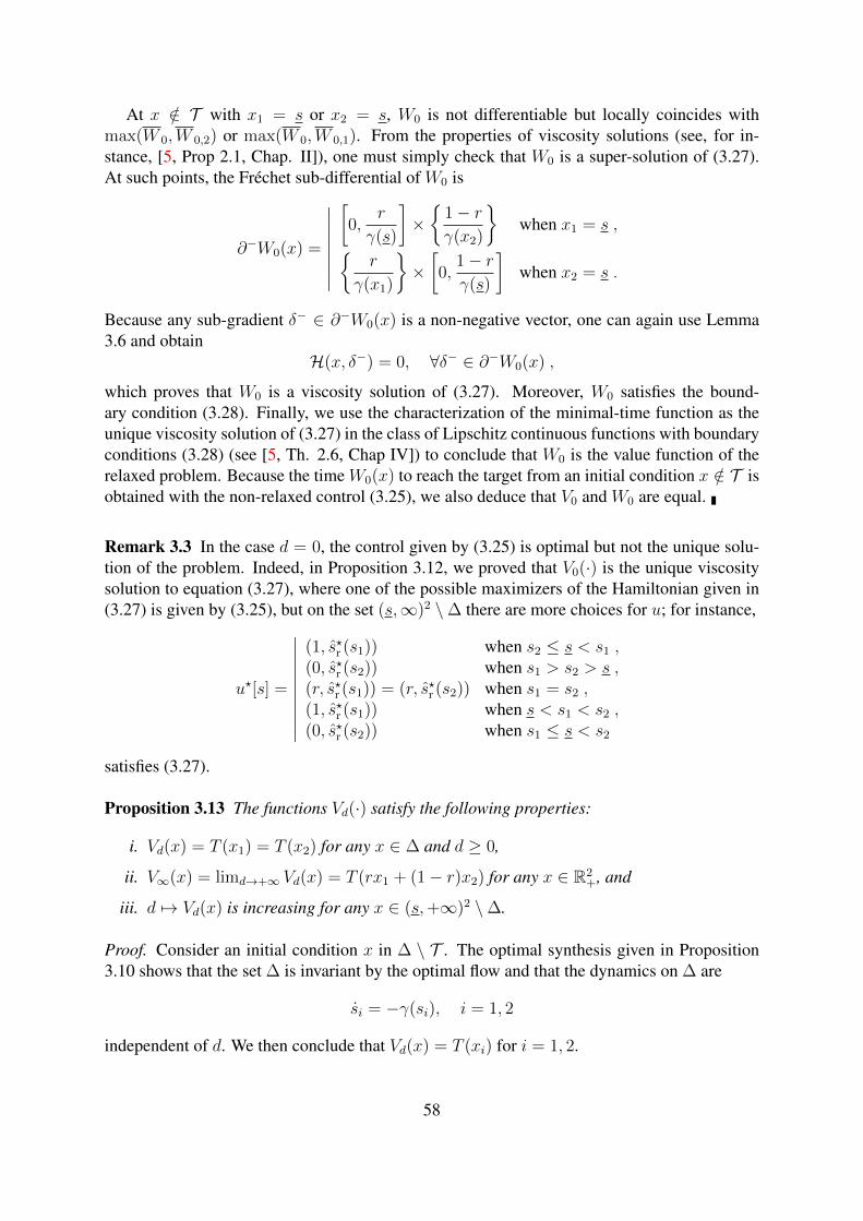
At x /∈ T with x1 = s or x2 = s, W0 is not differentiable but locally coincides withmax(W 0,W 0,2) or max(W 0,W 0,1). From the properties of viscosity solutions (see, for in-stance, [5, Prop 2.1, Chap. II]), one must simply check that W0 is a super-solution of (3.27).At such points, the Fréchet sub-differential of W0 is

∂−W0(x) =

∣∣∣∣∣∣∣∣[0,

r

γ(s)

]×

1− rγ(x2)

when x1 = s ,

r

γ(x1)

×[0,

1− rγ(s)

]when x2 = s .

Because any sub-gradient δ− ∈ ∂−W0(x) is a non-negative vector, one can again use Lemma3.6 and obtain

H(x, δ−) = 0, ∀δ− ∈ ∂−W0(x) ,

which proves that W0 is a viscosity solution of (3.27). Moreover, W0 satisfies the bound-ary condition (3.28). Finally, we use the characterization of the minimal-time function as theunique viscosity solution of (3.27) in the class of Lipschitz continuous functions with boundaryconditions (3.28) (see [5, Th. 2.6, Chap IV]) to conclude that W0 is the value function of therelaxed problem. Because the time W0(x) to reach the target from an initial condition x /∈ T isobtained with the non-relaxed control (3.25), we also deduce that V0 and W0 are equal.

Remark 3.3 In the case d = 0, the control given by (3.25) is optimal but not the unique solu-tion of the problem. Indeed, in Proposition 3.12, we proved that V0(·) is the unique viscositysolution to equation (3.27), where one of the possible maximizers of the Hamiltonian given in(3.27) is given by (3.25), but on the set (s,∞)2 \∆ there are more choices for u; for instance,

u?[s] =

∣∣∣∣∣∣∣∣∣∣(1, s?r (s1)) when s2 ≤ s < s1 ,(0, s?r (s2)) when s1 > s2 > s ,(r, s?r (s1)) = (r, s?r (s2)) when s1 = s2 ,(1, s?r (s1)) when s < s1 < s2 ,(0, s?r (s2)) when s1 ≤ s < s2

satisfies (3.27).

Proposition 3.13 The functions Vd(·) satisfy the following properties:

i. Vd(x) = T (x1) = T (x2) for any x ∈ ∆ and d ≥ 0,

ii. V∞(x) = limd→+∞ Vd(x) = T (rx1 + (1− r)x2) for any x ∈ R2+, and

iii. d 7→ Vd(x) is increasing for any x ∈ (s,+∞)2 \∆.

Proof. Consider an initial condition x in ∆ \ T . The optimal synthesis given in Proposition3.10 shows that the set ∆ is invariant by the optimal flow and that the dynamics on ∆ are

si = −γ(si), i = 1, 2

independent of d. We then conclude that Vd(x) = T (xi) for i = 1, 2.

58

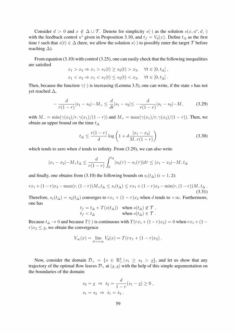
Consider d > 0 and x /∈ ∆ ∪ T . Denote for simplicity s(·) as the solution s(x, u?, d, ·)with the feedback control u? given in Proposition 3.10, and tf = Vd(x). Define t∆ as the firsttime t such that s(t) ∈ ∆ (here, we allow the solution s(·) to possibly enter the target T beforereaching ∆).

From equation (3.10) with control (3.25), one can easily check that the following inequalitiesare satisfied

x1 > x2 ⇒ x1 > s1(t) ≥ s2(t) > x2, ∀t ∈ [0, t∆] ,

x1 < x2 ⇒ x1 < s1(t) ≤ s2(t) < x2, ∀t ∈ [0, t∆] .

Then, because the function γ(·) is increasing (Lemma 3.5), one can write, if the state s has notyet reached ∆,

− d

r(1− r)|s1 − s2|−M+ ≤

d

dt|s1 − s2|≤ −

d

r(1− r)|s1 − s2|−M− (3.29)

with M− = min(γ(x2)/r, γ(x1)/(1− r)) and M+ = max(γ(x1)/r, γ(x2)/(1− r)). Then, weobtain an upper bound on the time t∆

t∆ ≤r(1− r)

dlog

(1 + d

|x1 − x2|M−r(1− r)

)(3.30)

which tends to zero when d tends to infinity. From (3.29), we can also write

|x1 − x2|−M+t∆ ≤d

r(1− r)

∫ t∆

0

|s2(τ)− s1(τ)|dτ ≤ |x1 − x2|−M−t∆

and finally, one obtains from (3.10) the following bounds on si(t∆) (i = 1, 2):

rx1 + (1− r)x2−max(r, (1− r))M+t∆ ≤ si(t∆) ≤ rx1 + (1− r)x2−min(r, (1− r))M−t∆ .(3.31)

Therefore, s1(t∆) = s2(t∆) converges to rx1 + (1 − r)x2 when d tends to +∞. Furthermore,one has

tf = t∆ + T (s(t∆)) when s(t∆) /∈ T ,tf < t∆ when s(t∆) ∈ T .

Because t∆ → 0 and because T (·) is continuous with T (rx1 + (1− r)x2) = 0 when rx1 + (1−r)x2 ≤ s, we obtain the convergence

V∞(x) = limd→+∞

Vd(x) = T (rx1 + (1− r)x2) .

Now, consider the domain D+ = s ∈ R2+ | s1 ≥ s2 > s, and let us show that any

trajectory of the optimal flow leaves D+ at (s, s) with the help of this simple argumentation onthe boundaries of the domain:

s2 = s ⇒ s2 =d

1− r(s1 − s) ≥ 0 ,

s1 = s2 ⇒ s1 = s2 .

59

It is convenient to consider the variable s = rs1 + (1 − r)s2, whose optimal dynamics in D+

are simply˙s(t) = −γ(s1(t)) , t ∈ [0, tf ] . (3.32)

Because s(·) is strictly decreasing with time, an optimal trajectory in D+ can be parameterizedby the fictitious time

τ(t) = rx1 + (1− r)x2 − s(t) , t ∈ [0, tf ] (3.33)

(where x is an initial condition in D+). The variable s1(·) is then a solution of the scalarnon-autonomous dynamics

ds1

dτ= fd(τ, s1) =

∣∣∣∣∣∣ −1

r− ds1 + τ − (rx1 + (1− r)x2)

r(1− r)γ(s1)when s1 + τ > rx1 + (1− r)x2 ,

−1 when s1 + τ = rx1 + (1− r)x2 ,

with the terminal fictitious time

τf = rx1 + (1− r)x2 − s .

Notice that τf is independent of d. One then deduces the inequalities

d1 > d2 and s1 + τ > rx1 + (1− r)x2 =⇒ fd1(τ, s1) < fd2(τ, s1)

and thus,

d1 > d2 and x ∈ D+ \∆ =⇒ s1(x, u?, d1, τ) < s1(x, u?, d2, τ) , ∀τ ∈ [0, τf ] . (3.34)

Finally, from equations (3.32) and (3.33), the time to reach the target can be expressed as

tf =

∫ τf

0

dτ

γ(s1(τ)). (3.35)

Because the function γ(·) is increasing and because τf is independent of d, one can concludefrom (3.34) and (3.35) that

d1 > d2 and x ∈ D+ \∆ =⇒ Vd1(x) > Vd2(x) .

The case of initial conditions in D− \∆, with D− = s ∈ R2+ | s2 ≥ s1 > s, is symmetric.

Remark 3.4 The tightness V∞−V0 of the bounds on the value function Vd on (s,+∞)2 \∆ isrelated to the concavity of the function T (·) on (s,+∞) (the less the concavity maxσ∈[s,+∞)|T

′′(σ)|

is, the tighter the bounds are).

The bounds V0 ≤ Vd < V∞ that are satisfied on the set (s,+∞)2 \ ∆ are not necessarilysatisfied outside this set: for x outside the target but such that rx1 + (1 − r)x2 < s, one hasV∞(x) = 0 and V0(x) > 0. Therefore, we conclude that a large diffusion negatively impactsthe time to treat the resource when both zones are initially polluted; however, when one of thetwo zones is initially under the pollution threshold, a large diffusion could positively impactthe duration of the treatment.

60

3.6 Numerical illustrations

We consider the Monod (or Michaelis-Menten) growth function, which is quite popular in bio-processes and which satisfies Assumption 3.1:

µ(s) = µmaxs

Ks + s,

with the parameters µmax = 1[h−1] and Ks = 1[gl−1]. The corresponding function γ(·) isdepicted in Fig. 3.2. The threshold that defines the target has been chosen as s = 1[gl−1].

s [g/L]

µ

1

0.8

[1/h]

1 s [g/L]

[g/L/h]

γ

1

Figure 3.2. Graphs of µ(·) and corresponding γ(·).

Several optimal trajectories in the phase portrait are drawn in Fig. 3.3 for small and largevalues of the parameter d.

1

1 s1 [g/L]

s2 [g/L]

1

1 s1 [g/L]

s2 [g/L]

Figure 3.3. Optimal paths for d = 0.1[h−1] (left) and d = 10[h−1] (right) with r = 0.3.

Finally, level sets of the value functions V0 and V∞ are represented in Fig. 3.4.One can make the following observations concerning the influence of the diffusion on the

treatment duration, that we consider to be valuable from a practical viewpoint.

• When pollution is homogeneous, the best is to maintain it homogeneous, and the treat-ment time is then independent of the diffusion.

• A high diffusion is favorable for having fast treatments when initial concentrations arestrongly different for the two zones. Typically, when the pollutant concentration is below

61

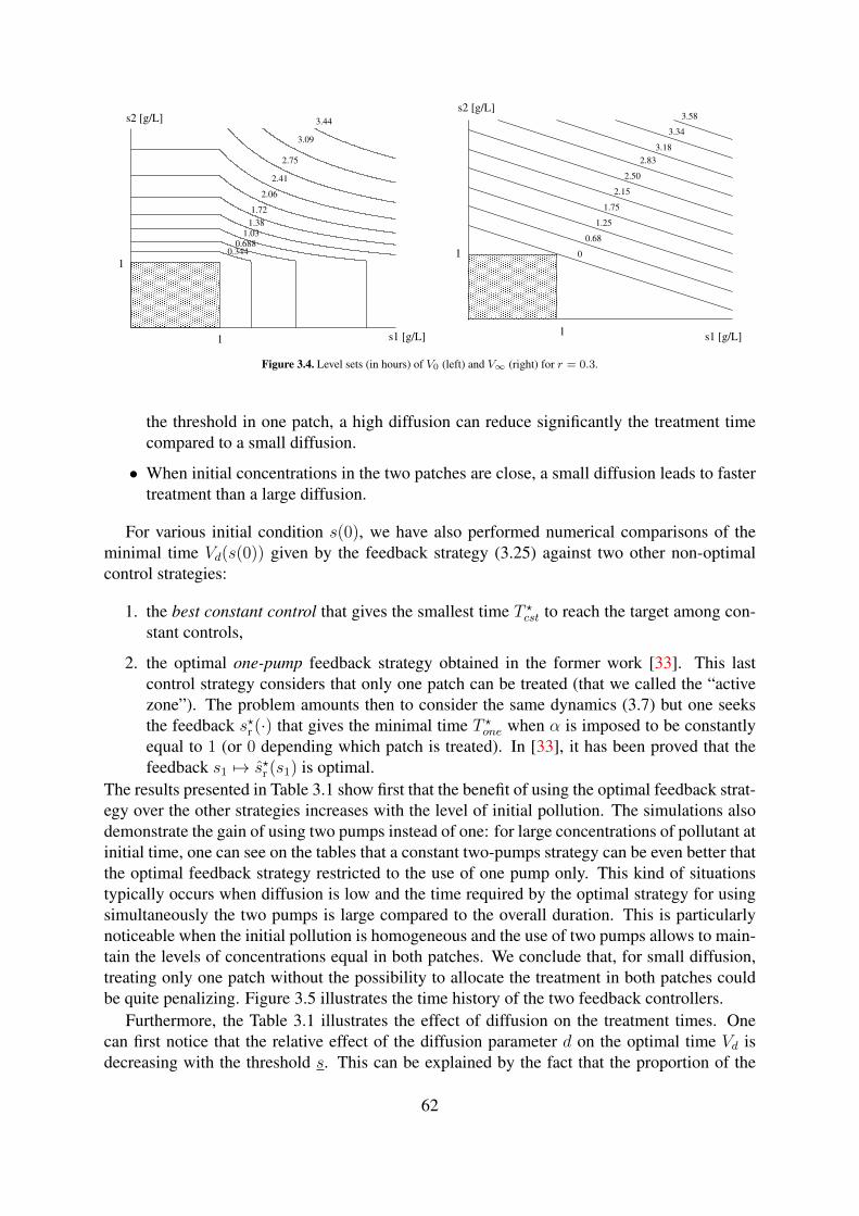
s1 [g/L]

s2 [g/L]

1

1

2.06

1.381.03

0.6880.344

2.75

1.72

3.44

3.09

2.41

3.58

3.34

3.18

2.83

2.50

2.15

1.75

1.25

0.68

0

1 s1 [g/L]

1

s2 [g/L]

Figure 3.4. Level sets (in hours) of V0 (left) and V∞ (right) for r = 0.3.

the threshold in one patch, a high diffusion can reduce significantly the treatment timecompared to a small diffusion.

• When initial concentrations in the two patches are close, a small diffusion leads to fastertreatment than a large diffusion.

For various initial condition s(0), we have also performed numerical comparisons of theminimal time Vd(s(0)) given by the feedback strategy (3.25) against two other non-optimalcontrol strategies:

1. the best constant control that gives the smallest time T ?cst to reach the target among con-stant controls,

2. the optimal one-pump feedback strategy obtained in the former work [33]. This lastcontrol strategy considers that only one patch can be treated (that we called the “activezone”). The problem amounts then to consider the same dynamics (3.7) but one seeksthe feedback s?r (·) that gives the minimal time T ?one when α is imposed to be constantlyequal to 1 (or 0 depending which patch is treated). In [33], it has been proved that thefeedback s1 7→ s?r (s1) is optimal.

The results presented in Table 3.1 show first that the benefit of using the optimal feedback strat-egy over the other strategies increases with the level of initial pollution. The simulations alsodemonstrate the gain of using two pumps instead of one: for large concentrations of pollutant atinitial time, one can see on the tables that a constant two-pumps strategy can be even better thatthe optimal feedback strategy restricted to the use of one pump only. This kind of situationstypically occurs when diffusion is low and the time required by the optimal strategy for usingsimultaneously the two pumps is large compared to the overall duration. This is particularlynoticeable when the initial pollution is homogeneous and the use of two pumps allows to main-tain the levels of concentrations equal in both patches. We conclude that, for small diffusion,treating only one patch without the possibility to allocate the treatment in both patches couldbe quite penalizing. Figure 3.5 illustrates the time history of the two feedback controllers.

Furthermore, the Table 3.1 illustrates the effect of diffusion on the treatment times. Onecan first notice that the relative effect of the diffusion parameter d on the optimal time Vd isdecreasing with the threshold s. This can be explained by the fact that the proportion of the

62

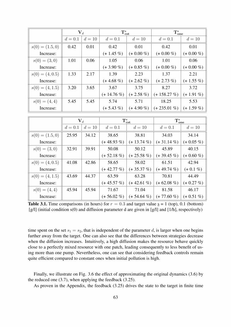
Vd T?cst T?

one

d = 0.1 d = 10 d = 0.1 d = 10 d = 0.1 d = 10

s(0) = (1.5, 0) 0.42 0.01 0.42 0.01 0.42 0.01Increase: (+ 1.45 %) (+ 0.00 %) (+ 0.00 %) (+ 0.00 %)

s(0) = (3, 0) 1.01 0.06 1.05 0.06 1.01 0.06Increase: (+ 3.90 %) (+ 0.85 %) (+ 0.00 %) (+ 0.00 %)

s(0) = (4, 0.5) 1.33 2.17 1.39 2.23 1.37 2.21Increase: (+ 4.68 %) (+ 2.62 %) (+ 2.73 %) (+ 1.55 %)

s(0) = (4, 1.5) 3.20 3.65 3.67 3.75 8.27 3.72Increase: (+ 14.76 %) (+ 2.58 %) (+ 158.27 %) (+ 1.91 %)

s(0) = (4, 4) 5.45 5.45 5.74 5.71 18.25 5.53Increase: (+ 5.43 %) (+ 4.90 %) (+ 235.01 %) (+ 1.59 %)

Vd T?cst T?

one

d = 0.1 d = 10 d = 0.1 d = 10 d = 0.1 d = 10

s(0) = (1.5, 0) 25.95 34.12 38.65 38.81 34.03 34.14Increase: (+ 48.93 %) (+ 13.74 %) (+ 31.14 %) (+ 0.05 %)

s(0) = (3, 0) 32.91 39.91 50.08 50.12 45.89 40.15Increase: (+ 52.18 %) (+ 25.58 %) (+ 39.45 %) (+ 0.60 %)

s(0) = (4, 0.5) 41.08 42.86 58.65 58.02 61.51 42.94Increase: (+ 42.77 %) (+ 35.37 %) (+ 49.74 %) (+ 0.1 %)

s(0) = (4, 1.5) 43.69 44.37 63.59 63.28 70.81 44.49Increase: (+ 45.57 %) (+ 42.61 %) (+ 62.08 %) (+ 0.27 %)

s(0) = (4, 4) 45.94 45.94 71.67 71.04 81.58 46.17Increase: (+ 56.02 %) (+ 54.64 %) (+ 77.60 %) (+ 0.51 %)

Table 3.1. Time comparisons (in hours) for r = 0.3 and target value s = 1 (top), 0.1 (bottom)[g/l] (initial condition s(0) and diffusion parameter d are given in [g/l] and [1/h], respectively)

time spent on the set s1 = s2, that is independent of the parameter d, is larger when one beginsfurther away from the target. One can also see that the differences between strategies decreasewhen the diffusion increases. Intuitively, a high diffusion makes the resource behave quicklyclose to a perfectly mixed resource with one patch, leading consequently to less benefit of us-ing more than one pump. Nevertheless, one can see that considering feedback controls remainquite efficient compared to constant ones when initial pollution is high.

Finally, we illustrate on Fig. 3.6 the effect of approximating the original dynamics (3.6) bythe reduced one (3.7), when applying the feedback (3.25).

As proven in the Appendix, the feedback (3.25) drives the state to the target in finite time

63

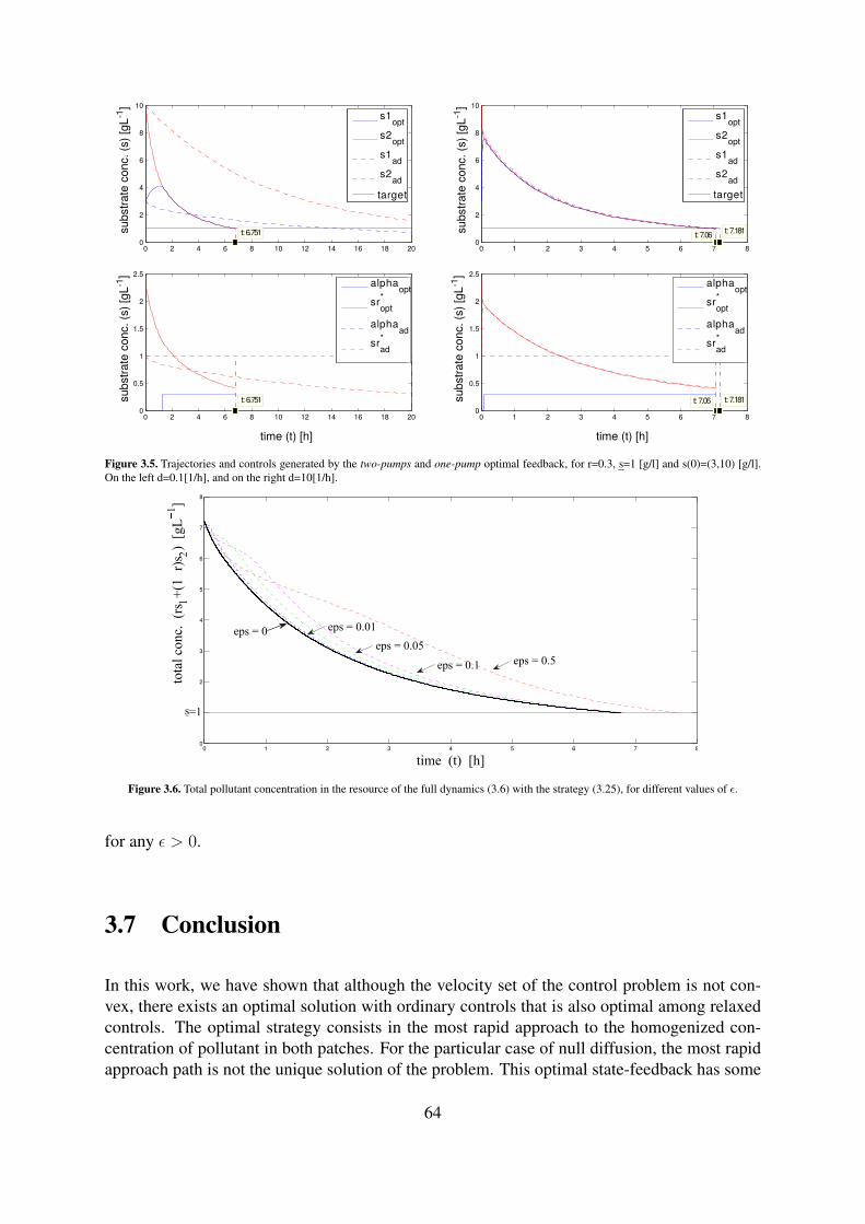
0 2 4 6 8 12 14 16 18 2010 0 1 2 3 4 5 6 7 80

2

4

6

8

10

t: 6.751substr

ate

conc. (s

) [g

L-1

]s1

opt

s2opt

s1ad

s2ad

target

0

2

4

6

8

10

t: 7.06t: 7.181

s1opt

s2opt

s1ad

s2ad

target

0 2 4 6 8 10 12 14 16 18 200

0.5

1

1.5

2

2.5

t: 6.751

alphaopt

sr*

opt

alphaad

sr*

ad

0 1 2 3 4 5 6 7 80

0.5

1

1.5

2

2.5

t: 7.06 t: 7.181

time (t) [h] time (t) [h]

alphaopt

sr*

opt

alphaad

sr*

ad

substr

ate

conc. (s

) [g

L-1

]

substr

ate

conc. (s

) [g

L-1

]substr

ate

conc. (s

) [g

L-1

]Figure 3.5. Trajectories and controls generated by the two-pumps and one-pump optimal feedback, for r=0.3, s=1 [g/l] and s(0)=(3,10) [g/l].On the left d=0.1[1/h], and on the right d=10[1/h].

0 1 2 3 4 5 6 7 80

2

3

4

5

6

7

8

time (t) [h]

tota

l co

nc.

(r

s 1+

(1r)

s 2)

[gL

1]

eps = 0 eps = 0.01

eps = 0.05

eps = 0.1 eps = 0.5

s=1

Figure 3.6. Total pollutant concentration in the resource of the full dynamics (3.6) with the strategy (3.25), for different values of ε.

for any ε > 0.

3.7 Conclusion

In this work, we have shown that although the velocity set of the control problem is not con-vex, there exists an optimal solution with ordinary controls that is also optimal among relaxedcontrols. The optimal strategy consists in the most rapid approach to the homogenized con-centration of pollutant in both patches. For the particular case of null diffusion, the most rapidapproach path is not the unique solution of the problem. This optimal state-feedback has some

64

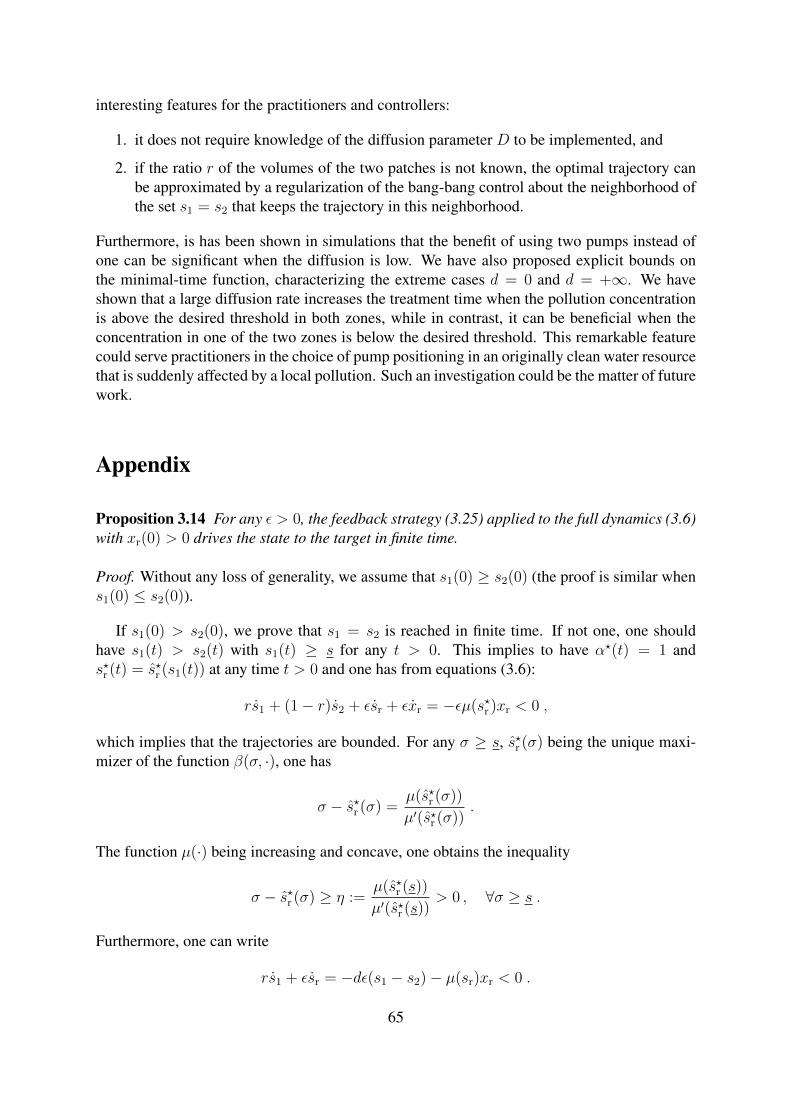
interesting features for the practitioners and controllers:

1. it does not require knowledge of the diffusion parameter D to be implemented, and

2. if the ratio r of the volumes of the two patches is not known, the optimal trajectory canbe approximated by a regularization of the bang-bang control about the neighborhood ofthe set s1 = s2 that keeps the trajectory in this neighborhood.

Furthermore, is has been shown in simulations that the benefit of using two pumps instead ofone can be significant when the diffusion is low. We have also proposed explicit bounds onthe minimal-time function, characterizing the extreme cases d = 0 and d = +∞. We haveshown that a large diffusion rate increases the treatment time when the pollution concentrationis above the desired threshold in both zones, while in contrast, it can be beneficial when theconcentration in one of the two zones is below the desired threshold. This remarkable featurecould serve practitioners in the choice of pump positioning in an originally clean water resourcethat is suddenly affected by a local pollution. Such an investigation could be the matter of futurework.

Appendix

Proposition 3.14 For any ε > 0, the feedback strategy (3.25) applied to the full dynamics (3.6)with xr(0) > 0 drives the state to the target in finite time.

Proof. Without any loss of generality, we assume that s1(0) ≥ s2(0) (the proof is similar whens1(0) ≤ s2(0)).

If s1(0) > s2(0), we prove that s1 = s2 is reached in finite time. If not one, one shouldhave s1(t) > s2(t) with s1(t) ≥ s for any t > 0. This implies to have α?(t) = 1 ands?r (t) = s?r (s1(t)) at any time t > 0 and one has from equations (3.6):

rs1 + (1− r)s2 + εsr + εxr = −εµ(s?r )xr < 0 ,

which implies that the trajectories are bounded. For any σ ≥ s, s?r (σ) being the unique maxi-mizer of the function β(σ, ·), one has

σ − s?r (σ) =µ(s?r (σ))

µ′(s?r (σ)).

The function µ(·) being increasing and concave, one obtains the inequality

σ − s?r (σ) ≥ η :=µ(s?r (s))

µ′(s?r (s))> 0 , ∀σ ≥ s .

Furthermore, one can write

rs1 + εsr = −dε(s1 − s2)− µ(sr)xr < 0 .

65

Thus rs1 + εsr is decreasing and has a limit when t tends to +∞. Since the trajectories arebounded, rs1 + εsr is uniformly continuous, and we conclude by Barbalat’s Lemma (see forinstance [49]) that rs1+εsr converges to 0, which implies that the positive quantities s1−s2 andµ(sr)xr have to converge also to 0. Notice that sr = 0 implies sr = µ(s?r )s1 > µ(s?r (s))s > 0.So sr cannot tend to 0 and xr has necessarily to converge to 0. Write now the dynamics

d

dt(s1 − sr) = −

(1 +

ε

r

)µ(s?r )(s1 − sr)− d

ε

r(s1 − s2)− µ(sr)xr ,

where µ(s?r ) > µ(s?r (s)) > 0 and d εr(s1 − s2) − µ(sr)xr tends to 0. Thus, there exists a time

T > 0 large enough such that

sr(t) > s1(t)− η ≥ s?r (t) , ∀t > T ,

which implies to have µ(sr)− µ(s?r ) > 0 for large t, thus a contradiction with the convergenceof xr to 0.

Clearly the feedback (3.25) leaves the set s1 = s2 invariant. Denote for simplicity sl =s1 = s2, and write

sl + εsr + εxr = −εµ(s?r )xr < 0 .

Trajectories are thus bounded, and by Barbalat’s Lemma one obtains that µ(s?r )xr tends to 0.We prove now that sl has to reach s in finite time. If not, µ(s?r (t)) > µ(s) for any time and xr

tends to zero. Write the dynamics

d

dt(sl − sr) = −(1 + ε)µ(s?r )(sl − sr) + µ(sr)xr .

As before, we deduce that there exits a time T ′ > 0 such that

sr(t) > sl(t)− η ≥ s?r (t) , ∀t > T ′ ,

leading to a contradiction with the convergence of xr to 0.

66

Chapter 4

Minimal-time bioremediation of naturalwater resources with gradient of pollutant

This chapter corresponds to an ongoing work.

4.1 Introduction

The fight against eutrophication of lakes and natural reservoirs (that is, the excessive develop-ment of phytoplankton associated with an excess of nutrients) constitutes a major challenge.This ecological issue has given rise to many studies over the last 30 years (see, for instance, thesurveys [34] or [75] and the references herein). To remediate eutrophication, various techniquessuch as bio-manipulation or ecological control have been proposed for mitigation. A commonpoint across the proposed remediation approaches is that they are usually based on "biotic" ac-tions on the lake trophic chain dedicated to the restoration of equilibrium in local ecosystems.To do so, most studies are based on empirical knowledge. However, since the 1970s, the use ofeutrophication models (ranging from heuristic data-based models at a steady state to more re-cent dynamic mass-balance-based models) together with optimal control techniques have beenproposed ([29] and references herein).

Since the pioneering work by [22], the optimization of bioreactor operation has receivedgreat attention in the literature; see [2, 3, 67] for reviews of the different optimization techniquesthat have been used in bioprocesses. Among them, the theory of optimal control has provento be a generic tool for deriving practical optimal rules [43, 71, 72]. The optimal control ofcontinuous processes usually involves a two-step procedure. First, the optimal steady stateis determined as a nominal set point that maximizes a criterion [76, 77]. The benefit of o-perating a periodic control about the nominal point can be analyzed [1, 69]. Then, a controlstrategy that drives the state about the nominal set point from any initial condition is searchedfor [50], possibly in the presence of model uncertainty using extremum seeking techniques[6, 54, 84, 86].

67

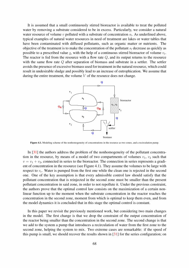
It is assumed that a small continuously stirred bioreactor is available to treat the pollutedwater by removing a substrate considered to be in excess. Particularly, we consider a naturalwater resource of volume v polluted with a substrate of concentration sl. As underlined above,typical examples of natural water resources in need of treatment are lakes or water tables thathave been contaminated with diffused pollutants, such as organic matter or nutrients. Theobjective of the treatment is to make the concentration of the pollutant sl decrease as quickly aspossible to a prescribed value s, with the help of a continuous stirred bioreactor of volume vr.The reactor is fed from the resource with a flow rate Q, and its output returns to the resourcewith the same flow rate Q after separation of biomass and substrate in a settler. The settleravoids the presence of excessive biomass used for treatment in the natural resource, which couldresult in undesirable sludge and possibly lead to an increase of eutrophication. We assume thatduring the entire treatment, the volume V of the resource does not change.

Q

rv

s , xrr

biomass

Q

Q

bioreactor

settler

s2

1v

2v

Q QR

s1

QR

Figure 4.1. Modeling scheme of the nonhomogeneity of concentrations in the resource as two zones, and a recirculation pump.

In [31] the authors address the problem of the nonhomogeneity of the pollutant concentra-tion in the resource, by means of a model of two compartments of volumes v1, v2 such thatv = v1 + v2, connected in series to the bioreactor. The connection in series represents a gradi-ent of concentration in the resource (see Figure 4.1). They assume the volumes to be large withrespect to vr. Water is pumped from the first one while the clean one is rejected in the secondone. One of the key assumption is that every admissible control law should satisfy that thepollutant concentration that is reinjected in the second zone must be smaller than the presentpollutant concentration in said zone, in order to not repollute it. Under the previous constraint,the authors prove that the optimal control law consists on the maximization of a certain non-linear function up to the moment when the substrate concentration in the reactor reaches theconcentration in the second zone, moment from which is optimal to keep them even, and fromthe model dynamics it is concluded that in this stage the optimal control is constant.

In this paper we revisit the previously mentioned work, but considering two main changesin the model. The first change is that we drop the constraint of the output concentration ofthe reactor being smaller than the concentration in the second zone. The second change is thatwe add to the system a pump that introduces a recirculation of water from the first zone to thesecond zone, helping the system to mix. Two extreme cases are remarkable: if the speed ofthis pump is small, we should recover the results shown in [31] for the series configuration; on

68

the other hand, if the speed of this pump is too high, we should recover the homogeneous case(also studied in [31]). We consider the speed of the pump QR as a new control parameter.

This paper is organized as follows. In Section 4.2, we introduce the mathematical model,and definitions and assumptions are presented. In Section 4.3 the minimal time optimal con-trol problem is introduced and the optimal control is charaterized. Section 4.4 is devoted tonumerical simulations and discussion.

4.2 Definitions and preliminaries

In what follows, we denote by R the set of real numbers, R+ and R?+ the sets of nonnegative

and positive real numbers respectively. Analogously, R− and R?− are the sets of nonpositive

and negative real numbers respectively.

For the time evolution of the concentrations of pollutant si, i = 1, 2, in the two zones of theresource, by means of a mass balance we obtain the equations:

s1 =Q+QR

v1

(s2 − s1),

s2 =Q

v2

(sr − s2) +QR

v2

(s1 − s2),

(4.1)

where the volumes vi, i = 1, 2 are assumed to be constant, Q is the flow rate of the pump thatconnects the first zone with the bioreactor, and QR is the flow rate of the pump that reinjectswater from the zone 1 to the zone 2 (see Figure 4.1).

We consider the usual chemostat model to describe the dynamics of the bioreactor [73]:sr = −µ(sr)xr +

Q

vr

(s1 − sr),

xr = µ(sr)xr −Q

vr

xr

(4.2)

where sr and xr indicate the concentrations of substrate and biomass inside the bioreactor,respectively.

The growth rate function µ(·) fulfills the following properties.

Assumption 4.1 The growth function µ(·) is defined on R+, continuously differentiable on R?+,

increasing, concave, and satisfies µ(0) = 0.

Since we have supposed that v1 and v2 are considerably larger than vr, the process has a slow-fast dynamic in which the slow variables are (s1, s2) and the fast variables are (xr, sr). Thisimplies that the substrate and biomass concentrations present in the bioreactor can be approxi-mated in the slow time scale by a quasi-stationary state (x?r , s

?r ) = (x?r (s1, s2, Q), s?r (s1, s2, Q))

69

satisfying the following relations:

µ(s?r ) =Q

vr

, x?r = s1 − s?r . (4.3)

Under Assumption 4.1, system (4.3) has unique solution for s?r ∈ [0, s1]. Notice that thisimposes a constraint on s?r for the positivity of the biomass concentration in the bioreactor. Forsimplicity, we keep the notation sr instead of s?r for the concentration of equilibrium in thebioreactor. Denoting αi = vr/vi (i = 1, 2) results in the following dynamics:

s1 =

(α1µ(sr) +

QR

v1

)(s2 − s1)

s2 = α2µ(sr)(sr − s2) +QR

v2

(s1 − s2).

(4.4)

From now on, we work with the dynamics (4.4). Notice that the problem can be reformu-lated with the controls (sr, QR) instead of (Q,QR), but this formulation has the inconvenientthat the set where the control takes values depends of the state variable. Nevertheless, we canmake a change of variable of the form sr = ws1, with w ∈ [0, 1] and take (w,QR) as the controlvariable instead of (Q,QR). We keep sr as variable when there is no confusion, always keepingin mind that sr = ws1. Define the set of admissible controls

U =u = (w,QR) : R+ → R2

+ |w(t) ∈ [0, 1], QR ∈ [0, QR] for all t ∈ R+

.

Lemma 4.2 The setD := s ∈ R2+ | s1 ≥ s2 is positively invariant for any admissible control

u ∈ U .

Proof. Suppose s = (s1, s2) ∈ D and a control u ∈ U . By the continuity of the solutions of(4.4), the only way to leave the set D is through s1 = s2. The equation that s1 − s2 satisfy is

s1 − s2 = −(α1µ(sr) +QR

(1

v1

+1

v2

))(s1 − s2)− α2µ(sr)(sr − s2).

Then, if s1 = s2, we have

s1 − s2 = −α2µ(sr)(sr − s2) = α2µ(sr)(s1 − sr) > 0,

so the set D cannot be abandoned.

4.3 Optimal control problem

Due to Lemma 4.2 we may suppose that the initial condition for the process belongs to the setD. Consequently, the target set can be considered as

T := (s1, s2) ∈ R2+ | s1 ≤ s. (4.5)

70

The optimization problem consists of driving down the concentration of the resource to aprescribed value s > 0 from an initial condition z ∈ D in minimal time:

(P) minu∈Ut ≥ 0 | s(t) ∈ T , s(0) = z .

The Hamiltonian of the problem is

H(s, λ;u) = −1 + µ(ws1) [α1λ1(s2 − s1) + α2λ2(ws1 − s2)] +QR(s1 − s2)

[−λ1

v1

+λ2

v2

],

that is maximized along the optimal trajectory; if uopt = (wopt, QoptR ) is a solution of problem

(P), the adjoint state λ = (λ1, λ2) satisfies

λ1 = λ1

(α1µ(wopts1) +

QoptR

v1

+ α1woptµ′(wopts1)(s1 − s2)

)−λ2

(Qopt

R

v2

+ α2woptµ(wopts1) + α2w

optµ′(wopts1)(wopts1 − s2)

),

λ2 = −λ1

(α1µ(wopts1) +

QoptR

v1

)+ λ2

(α2µ(wopts1) +

QoptR

v2

),

(4.6)

with the transversality conditions

λ1(Topt) < 0 , λ2(Topt) = 0. (4.7)

Regarding the behavior of the adjoint states, we have the following lemma.

Lemma 4.3 Along any admissible extremal, one has λ1(t) < 0 for any t ≤ Topt, and λ2(t) < 0for any t < Topt.

Proof. If one writes the adjoint equations (4.6) as λi = φi(t, λ1, λ2) (i = 1, 2), one can no-tice that the partial derivatives ∂jφi (i 6= j) are non-positive. From the theory of monotonedynamical systems (see for instance [74]), the dynamics (4.6) is thus competitive or, equiva-lently, cooperative in backward time. As the transversality conditions (4.7) gives λi(Topt) ≤ 0(i = 1, 2), we deduce by the property of monotone dynamics that one should have λi(t) ≤ 0(i = 1, 2) for any t ≤ Topt. Moreover, λ = 0 is an equilibrium of (4.6) and λ(Topt) has to bedifferent from 0 at any time t ≤ Topt. Then, λi(t) (i = 1, 2) cannot be simultaneously equal tozero. If there exists t < Topt and i ∈ 1, 2 such that λi(t) = 0, then one should have λj(t) < 0for j 6= i. However, µ(·) being positive and QR ≥ 0 implies λi(t) ≥ 0; moreover, if λ1(t) = 0,then λ1(t) ≥ 0 and we contradict the transversality condition λ1(Topt) < 0; in the same way, ifλ2(t) = 0, then λ2(t) > 0 and we contradict the transversality condition λ2(Topt) = 0.

Consider the following function

γ(t) =α2λ2(t)

α1λ1(t), (4.8)

71

whose time derivative γ fulfills

γ =µ(wopts1) ((α2 − α1)γ − α2) +Qopt

R

v1

(α2

α1

+ γ

)(−1 + γ)

+ woptα1γ(−µ′(wopts1)(s1 − s2) + γµ(wopts1) + γµ′(wopts1)(wopts1 − s2)

),

(4.9)

with final condition γ(Topt) = 0. Also note that γ = 0 implies γ < 0 and therefore γ(t) > 0for any t ∈ [0, Topt). With this new variable, we can rewrite the Hamiltonian as

H(s, λ1, γ;u) = −1− α1λ1(s1 − s2)µ(ws1)

[1 + γ

s2 − ws1

s1 − s2

]+QR(s1 − s2)

−λ1

v1

[1− γ] ,

(4.10)For s1 > s2 > 0, w ∈ [0, 1], and γ > 0, we define the following functions

φ(s1, s2, γ, w) = µ(ws1)

[1 + γ

s2 − ws1

s1 − s2

], (4.11)

ψ(s1, s2, γ) = µ′(s1)(1− γ)− γ µ(s1)

s1 − s2

. (4.12)

Notice that ψ(s1, s2, γ) = 1s1

∂∂wφ(s1, s2, γ, w)|w=1. When s1 > s2 and γ > 0, the max-

imization of the Hamiltonian with respect to (w,QR) ∈ [0, 1] × [0, QR] is equivalent to themaximization of the functions w 7→ φ(s1, s2, γ, w) with w ∈ [0, 1] and QR 7→ (1− γ)QR withQR ∈ [0, QR]. Such maximum wopt is unique, as we see in Lemma 4.4.

Lemma 4.4 Under Assumption 4.1, for s1 > s2 > 0 and γ > 0, the function φ(s1, s2, γ, ·) isstrictly concave on the interval

[0, s1−s2

γs1+ s2

s1

].

Proof. Notice that the function φ can be written as

φ(s1, s2, γ, w) =γ

s1 − s2

µ(ws1) (c− ws1) , c :=s1 − s2

γ+ s2. (4.13)

Define the function β(s, sr) := µ(sr)(s − sr), (s, sr) ∈ R2+. This is a twice differentiable

function, and for fixed s > 0, the function sr 7→ β(s, sr) is positive on the interval (0, s),negative on (s,∞), and it is strictly concave in the interval [0, s]. Indeed,

∂2

∂s2r

β(s, sr) = µ′′(sr)(s− sr)− 2µ′(sr), (4.14)

which thanks to Assumption 4.1 in strictly negative. Taking s = c = s1−s2γ

+ s2, we see thatβ(c, ·) is strictly concave in the set [0, c], and using that sr = ws1 is a linear increasing functionof w we conclude that the function w 7→ β(c, ws1) is strictly concave in [0, c/s1].

The previous lemma allows to perform an analysis of the necesary conditions for the optimalcontrol values. In the following lemma we characterize the possible values for an optimalcontrol u? dependig on the functions ψ and γ.

72

Lemma 4.5 For fixed (s, λ1, γ) ∈ R2+ × R− × R+, with s1 > s2 > 0 and γ > 0, the value

u? = (w?, Q?R) that maximizes the function u 7→ H(s, λ1, γ;u) (with H as in (4.10)) are the

following:

1. when γ ≥ 1, Q?R = 0 and w? is the unique solution of

∂

∂wφ(s1, s2, γ, w

?) = 0, (4.15)

2. when γ < 1 and ψ(s, γ) < 0, Q?R = QR and w? is the solution of (4.15),

3. when γ < 1 and ψ(s, γ) ≥ 0, Q?R = QR and w? = 1.

Proof. Consider again the function β defined in Lemma 4.4. The maximization of φ(s1, s2, γ, ·)is equivalent to the maximization of w 7→ β(c, ws1) in [0, 1], with c as in (4.13).

Consider first the case γ ≥ 1. This implies that s1 ≥ c, and then w? belongs to the interval(0, c/s1) (because in the interval (c/s1, 1] the function w 7→ β(c, ws1) is negative). In thisinterval the function w 7→ β(c, ws1) is differentiable and strictly concave (Lemma 4.4) andthen the maximizer w? is unique and satisfies w? < 1. We conclude that w? satisfies (4.15).

Now, we look at the case γ < 1. This implies that s1 < c, and we cannot straightforwardlyensure that w? < 1; nevertheless, depending on the sign of ψ(s1, s2, γ) we can distinguish twosituations: if ψ(s1, s2, γ) ≤ 0 we have that φ(s1, s2, γ, ·) is decreasing in the interval [1, c/s1]and consequently its maximum w? belongs to the interval (0, 1); in particular w? is unique andsatisfies (4.15). On the other hand, if ψ(s1, s2, γ) > 0, that means that in the interval [0, 1] thefunction φ(s1, s2, γ, ·) is increasing, being maximized in the extreme point w? = 1 (which isagain unique).

The variable Q?R maximizes a linear function which only depends on the sign of 1 − γ

(because s1 > s2 and by Lemma 4.3 we have λ1 < 0). If γ > 1, then 1− γ is negative and themaximum is the extreme point Q?

R = 0; if γ < 1, then 1 − γ is positive and the maximum isthe extreme point Q?

R = QR. Notice that singular arcs with respect to QR do not exist, becauseγ = 1 and γ = 0 imply s?r = 0, which can only happen if s1 = 0.

Remark 4.1 The previous lemma can be expressed in terms of the equilibrium substrate con-centration at the output of the bioreactor sr as

1. when γ ≥ 1, Q?R = 0 and s?r is the unique solution of

∂

∂sr

H(s1, s2, γ, s?r ) = 0, (4.16)

2. when γ < 1 and ψ(s, γ) < 0, Q?R = QR and s?r is the solution of (4.16),

3. when γ < 1 and ψ(s, γ) ≥ 0, Q?R = QR and s?r = s1.

73

In order to characterize the behavior of the optimal control uopt = (wopt, QoptR ) along time,

we need then to study the behavior of the function ψ as a function of time. The time derivativeof ψ is

ψ =

(µ′′(s1)(1− γ)− µ′(s1)

γ

s1 − s2

)s1 − µ(s1)

d

dt

[γ

s1 − s2

]− µ′(s1)γ,

where a straightforward calculation provides

d

dt

[γ

s1 − s2

]=α2µ(wopts1)

s1 − s2

[γ

(1− s2 − wopts1

s1 − s2

)− 1

]+

QoptR

v1(s1 − s2)

(γ2 + 2

α2

α1

γ − α2

α1

)+ γ

α1wopt

s1 − s2

(−µ′(wopts1)(s1 − s2) + γµ(wopts1) + γµ′(wopts1)(wopts1 − s2)

).

The full expression for ψ can be written as ψ = I1 + I2 + I3 + I4, where

I1 =

(−µ′′(s1)(1− γ) + µ′(s1)

γ

s1 − s2

)(α1µ(wopts1) +

QoptR

v1

)(s1 − s2),

I2 = −µ(s1)

(α2µ(wopts1)

s1 − s2

[γ

(1− s2 − wopts1

s1 − s2

)− 1

]+

QoptR

v1(s1 − s2)

(γ2 + 2

α2

α1

γ − α2

α1

)),

I3 = −µ′(s1)

(µ(wopts1) ((α2 − α1)γ − α2) +

QoptR

v1

(γ2 +

(α2

α1

− 1

)γ − α2

α1

)),

I4 = −γ α1wopt

s1 − s2

(−µ′(wopts1)(s1 − s2) + γµ(wopts1) + γµ′(wopts1)(wopts1 − s2)

)× (µ(s1) + µ′(s1)(s1 − s2)).

(4.17)

At the final time we have γ(Topt) = 0 (thus QoptR (Topt) = QR) and ψ(Topt) = µ′(s) > 0

(thus wopt(Topt) = 1); so there exists a time t? < Topt such that for all t ∈ (t?, Topt], we haveγ(t) < 1 and ψ(t) > 0. In terms of the optimal control uopt, by Lemma 4.5 this translatesinto Qopt

R (t) = QR and wopt(t) = 1 (equivalently soptr (t) = s1(t)) for all t in a time interval

(t?, Topt] before the final time.

Remark 4.2 The control QoptR takes its maximum value before wopt can reach its maximum

value. Indeed, if for some t > 0 we have γ(t) = 1, then ψ(t) < 0, so wopt(t) still belongs to theinterval (0, 1) (Lemma 4.5). In term of the substrate concentration at the output of the reactor,sopt

r (t) still belongs to the interval (0, s1(t)).

We have the two following lemmas concerning the behavior of the switching functions γand ψ.

Lemma 4.6 Suppose that at a certain time t† < Topt we have γ(t†) = 1. Then, for all t ∈(t†, Topt] we have γ(t) < 1.

74

Proof. Suppose that γ = 1. Then, evaluating in the expression of γ given in (4.9), we haveγ = −µ(sopt

r )α1 < 0. We conclude that once the set γ ≤ 1 is reached, it is never left.

Lemma 4.7 Suppose that at a certain time t† < Topt we have ψ(t†) = 0. Then, for allt ∈ (t†, Topt] we have ψ(t) > 0.

Proof. Supposeψ ≥ 0. Then γ belongs to the set [0, γmax(s)] where γmax(s) := µ′(s1)(s1−s2)µ′(s1)(s1−s2)+µ(s1)

<

1. According to the control rule given in Lemma 4.5, wopt = 1 and QoptR = QR. In this case,

the formula for ψ is

ψ =

(−µ′′(s1)(1− γ) + µ′(s1)

γ

s1 − s2

)(α1µ(s1) +

QR

v1

)(s1 − s2)

− µ(s1)

(α2µ(s1)

s1 − s2

(2γ − 1) + µ′(s1) ((α2 − α1)γ − α2)

)− QR

v1

(µ(s1)

s1 − s2

(γ2 + 2

α2

α1

γ − α2

α1

)+ µ′(s1)

(γ2 +

(α2

α1

− 1

)γ − α2

α1

))− γ α1

s1 − s2

(µ′(s1)(s1 − s2)(−1 + γ) + γµ(s1)) (µ(s1) + µ′(s1)(s1 − s2))

(4.18)

The previous expression corresponds to a concave function of second degree as function of γ;let us denote it by hs(γ). So, if we prove that hs is positive for γ = 0 and γ = γmax(s), weconclude that ψ ≥ 0. First, we take γ = 0, and compute

hs(0) = −µ′′(s1)

(α1µ(s1) +

QR

v1

)(s1 − s2) +

α2

α1

(µ(s1)

s1 − s2

+ µ′(s1)

)(α1µ(s1) +

QR

v1

),

which is positive. Now, we evaluate γ = γmax(s) in the formula of hs given by (4.18) (for easewe write γmax(s) as γmax), which gives as result hs(γmax) = I1 + I2 + I3 + I4, with

I1 =

(−µ′′(s1)(1− γmax) + µ′(s1)

γmax

s1 − s2

)(α1µ(s1) +

QR

v1

)(s1 − s2),

I2 = −µ(s1)

(α2µ(s1)

s1 − s2

(2γmax − 1) + µ′(s1) ((α2 − α1)γmax − α2)

),

I3 = −QR

v1

(µ(s1)

s1 − s2

(γ2

max + 2α2

α1

γmax −α2

α1

)+ µ′(s1)

(γ2

max +

(α2

α1

− 1

)γmax −

α2

α1

))I4 = −γmax

α1

s1 − s2

(µ′(s1)(s1 − s2)(−1 + γmax) + γmaxµ(s1)) (µ(s1) + µ′(s1)(s1 − s2)).

Since γmax < 1, we conclude that I1 > 0. Now, for the analysis of I2, we notice that

2γmax − 1 = 2µ′(s1)(s1 − s2)

µ′(s1)(s1 − s2) + µ(s1)− 1 =

µ′(s1)(s1 − s2)− µ(s1)

µ′(s1)(s1 − s2) + µ(s1)< 0,

the last inequality obtained from the fact that µ(·) is strictly concave and positive. We also have

(α2 − α1)γmax − α2 = α2(γmax − 1)− α1 < 0,

75

concluding that I2 > 0. For I3 we develop the quadratic expressions

γ2max + 2

α2

α1

γmax −α2

α1

=1

α1

(α1 + α2)µ′(s1)2(s1 − s2)2 − α2µ(s1)2

(µ′(s1)(s1 − s2) + µ(s1))2,

and

γ2max +

(α2

α1

− 1

)γmax −

α2

α1

= −µ(s1)

α1

α2µ(s1) + (α1 + α2)µ′(s1)(s1 − s2)

(µ′(s1)(s1 − s2) + µ(s1))2,

concluding that

I3 = QRα2

v1α1

1

s1 − s2

µ(s1)2

µ′(s1)(s1 − s2) + µ(s1),

is positive. Now, I4 can be written as

I4 = −γmaxα1

s1 − s2

(µ(s1) + µ′(s1)(s1 − s2))J,

withJ = µ′(s1)(s1 − s2)(−1 + γmax) + γmaxµ(s1)

= µ′(s1)(s1 − s2)

(−1 +

µ′(s1)(s1 − s2)

µ′(s1)(s1 − s2) + µ(s1)

)+

µ′(s1)(s1 − s2)

µ′(s1)(s1 − s2) + µ(s1)µ(s1) = 0.

Thus, we conclude that if γ ∈ [0, γmax], then ψ > 0.

Lemmas 4.6 and 4.7 summarize the behavior of any optimal control strategy uopt = (wopt, QoptR )

in terms of the state variable sopt, the adjoint variable γ, and the function ψ. We state this resultin the following proposition.

Proposition 4.8 Suppose that sopt is an optimal trajectory, associated to the optimal controluopt = (wopt, Qopt

R ). Then, there exist time instants 0 ≤ t1 < t2 < Topt such that

1. QoptR (t) = 0 and wopt(t) = w(sopt(t), γ(t)) a.e. t ∈ [0, t1], where w(s, γ) satisfies (4.15),

where t1 is the first time that γ(t) ≤ 1 (it may occur that t1 = 0),

2. QoptR (t) = QR and wopt(t) = w(sopt(t), γ(t)) a.e. t ∈ [t1, t2], where w(s, γ) satisfies

(4.15), where t2 is the first time in which ψ(t) ≥ 0;

3. QoptR (t) = QR and wopt(t) = 1 a.e. t ∈ [t2, Topt].

Proof. According to Pontryagin’s Maximum Principle, an optimal control uopt has to maximizefor a.e. t ∈ [0, Topt] time the Hamiltonian H given in (4.10) or, equivalently, since λ(t) ≤ 0and γ(t) ≥ 0 (Lemma 4.3), maximize the functions w 7→ φ(sopt(t), γ(t), w) with w ∈ [0, 1]and QR 7→ (1 − γ(t))QR with QR ∈ [0, QR]. Suppose γ(0) > 1 (otherwise, t1 = 0). Since γis continuous with γ(Topt) = 0, there exist a time instant t1 ≥ 0 such that γ(t1) = 1. For a.e.t ∈ [0, t1], point 1. of Lemma 4.5 is satisfied. For t > t1 Lemma 4.6 states that γ(t) < 1 andthen Lemma 4.5 states that for t ≥ t1, Qopt

R . Now, Remark 4.2 states that ψ(t1) < 0 and weknow that ψ(Topt) > 0, so there exists a time instant t2 < Topt such that ψ(t2) > 0 and t1 < t2.Lemma 4.7 says that a.e. t ∈ [t1, t2] point 2. of Lemma 4.5 holds, and a.e. t ∈ [t2, Topt] thepoint 3. of Lemma 4.5 holds.

76

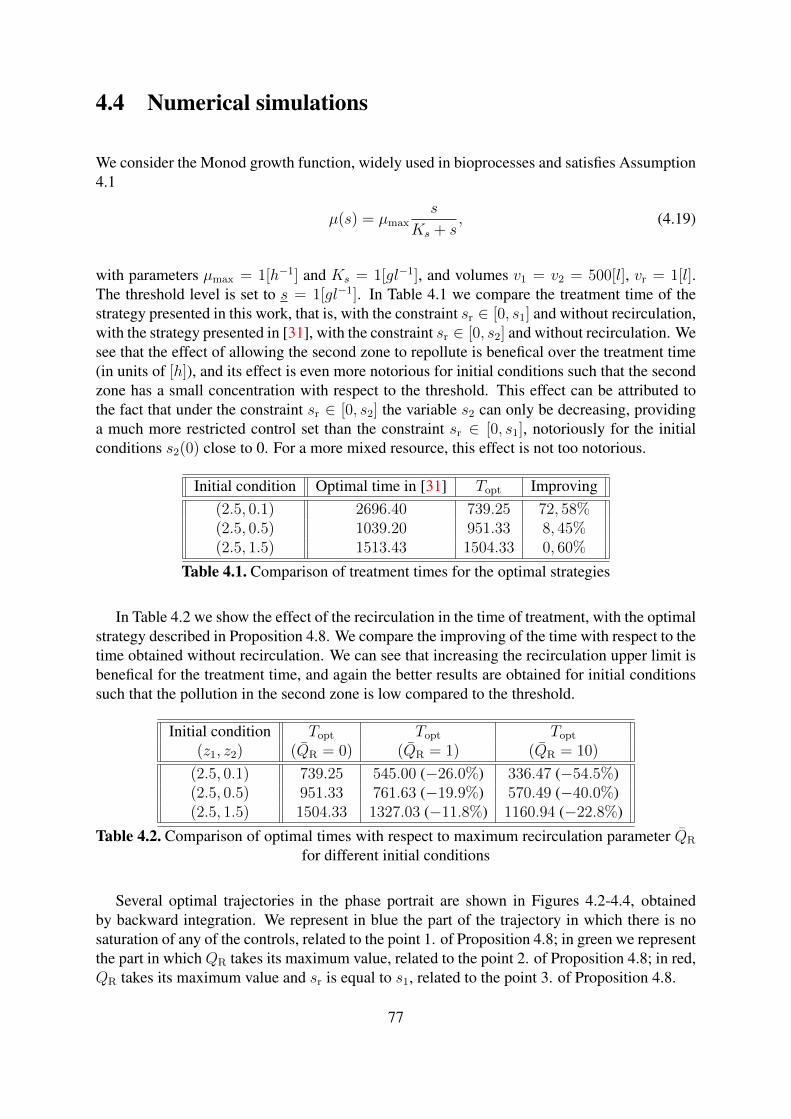
4.4 Numerical simulations

We consider the Monod growth function, widely used in bioprocesses and satisfies Assumption4.1

µ(s) = µmaxs

Ks + s, (4.19)

with parameters µmax = 1[h−1] and Ks = 1[gl−1], and volumes v1 = v2 = 500[l], vr = 1[l].The threshold level is set to s = 1[gl−1]. In Table 4.1 we compare the treatment time of thestrategy presented in this work, that is, with the constraint sr ∈ [0, s1] and without recirculation,with the strategy presented in [31], with the constraint sr ∈ [0, s2] and without recirculation. Wesee that the effect of allowing the second zone to repollute is benefical over the treatment time(in units of [h]), and its effect is even more notorious for initial conditions such that the secondzone has a small concentration with respect to the threshold. This effect can be attributed tothe fact that under the constraint sr ∈ [0, s2] the variable s2 can only be decreasing, providinga much more restricted control set than the constraint sr ∈ [0, s1], notoriously for the initialconditions s2(0) close to 0. For a more mixed resource, this effect is not too notorious.

Initial condition Optimal time in [31] Topt Improving(2.5, 0.1) 2696.40 739.25 72, 58%(2.5, 0.5) 1039.20 951.33 8, 45%(2.5, 1.5) 1513.43 1504.33 0, 60%

Table 4.1. Comparison of treatment times for the optimal strategies

In Table 4.2 we show the effect of the recirculation in the time of treatment, with the optimalstrategy described in Proposition 4.8. We compare the improving of the time with respect to thetime obtained without recirculation. We can see that increasing the recirculation upper limit isbenefical for the treatment time, and again the better results are obtained for initial conditionssuch that the pollution in the second zone is low compared to the threshold.

Initial condition Topt Topt Topt

(z1, z2) (QR = 0) (QR = 1) (QR = 10)

(2.5, 0.1) 739.25 545.00 (−26.0%) 336.47 (−54.5%)(2.5, 0.5) 951.33 761.63 (−19.9%) 570.49 (−40.0%)(2.5, 1.5) 1504.33 1327.03 (−11.8%) 1160.94 (−22.8%)

Table 4.2. Comparison of optimal times with respect to maximum recirculation parameter QR

for different initial conditions

Several optimal trajectories in the phase portrait are shown in Figures 4.2-4.4, obtainedby backward integration. We represent in blue the part of the trajectory in which there is nosaturation of any of the controls, related to the point 1. of Proposition 4.8; in green we representthe part in which QR takes its maximum value, related to the point 2. of Proposition 4.8; in red,QR takes its maximum value and sr is equal to s1, related to the point 3. of Proposition 4.8.

77

1 1.5 2 2.5 3 3.5 40

0.5

1

1.5

s1

[gL−1

]

s2

[gL

−1]

Phase portrait of optimal trajectories, QR = 0

Figure 4.2. Backward integration of the extremals, with QR = 0.

1 1.5 2 2.5 3 3.5 40

0.5

1

1.5

s1

[gL−1

]

s2

[gL

−1]

Phase portrait of optimal trajectories, QR = 1

Figure 4.3. Backward integration of the extremals, with QR = 1.

78

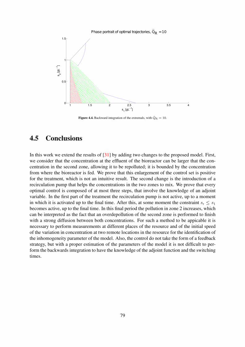
1 1.5 2 2.5 3 3.5 40

0.5

1

1.5

s1

[gL−1

]

s2

[gL

−1]

Phase portrait of optimal trajectories, QR = 10

Figure 4.4. Backward integration of the extremals, with QR = 10.

4.5 Conclusions

In this work we extend the results of [31] by adding two changes to the proposed model. First,we consider that the concentration at the effluent of the bioreactor can be larger that the con-centration in the second zone, allowing it to be repolluted; it is bounded by the concentrationfrom where the bioreactor is fed. We prove that this enlargement of the control set is positivefor the treatment, which is not an intuitive result. The second change is the introduction of arecirculation pump that helps the concentrations in the two zones to mix. We prove that everyoptimal control is composed of at most three steps, that involve the knowledge of an adjointvariable. In the first part of the treatment the recirculation pump is not active, up to a momentin which it is activated up to the final time. After this, at some moment the constraint sr ≤ s1

becomes active, up to the final time. In this final period the pollution in zone 2 increases, whichcan be interpreted as the fact that an overdepollution of the second zone is performed to finishwith a strong diffusion between both concentrations. For such a method to be appicable it isnecessary to perform measurements at different places of the resource and of the initial speedof the variation in concentration at two remote locations in the resource for the identification ofthe inhomogeneity parameter of the model. Also, the control do not take the form of a feedbackstrategy, but with a proper estimation of the parameters of the model it is not difficult to per-form the backwards integration to have the knowledge of the adjoint function and the switchingtimes.

79

Chapter 5

Stochastic modelling of sequencing batchreactors for wastewater treatment

This chapter corresponds to an ongoing work.

5.1 Introduction

Sequencing batch reactors (SBR) are a biological water treatment system. They are widely usedfor industrial and municipal wastewater. They are a time-oriented system with flow, energyinput, and tank volume varying according to some prescribed strategy. In its most basic form,the SBR system consists of one or many tanks that operate in a fill-and-draw basis: the tankis filled during a discrete period of time and then operated as a batch reactor. The essentialdifference between the SBR and a conventional continuous bioreactor is that inside each tankfunctions as equalization, aeration, and sedimentation can be performed in a time sequencerather than a spatial sequence. This kind of waste-water treatment system is well described in[44, 45].

The cycle of operation for each tank in an SBR system consists of five basic operatingmodes performed in a time sequence: fill, react, settle, draw, and idle modes. During fill modethe wastewater is received in the tank; during react mode the desired reactions take place;in settle mode the microorganisms are separated from the treated water; in draw mode thetreated effluent is discharged, and idle mode corresponds to the period comprised between thedischarge of the tank and its refilling. The time of a cycle is the total time between the beginningof fill up to the end of idle. The necessary time to achieve the total cycle may be long, and thismay be economically expensive. On the other hand, one should expect that a longer treatmenttime leads to a better depollution level.

The problem consists in the minimization of the time of the treatment in each cycle ofoperation, in which the time associated to draw and idle modes is fixed. Then, by changing

80

the input flow rate it is possible to control the time of treatment, in particular, the durationtime of the fill mode. The tank has a maximum volume, and it is reasonable to establish asone of the goals to treat the maximum possible amount of wastewater in each cycle. Thisproblem was studied in [60] for the single-species case with monotonic and nonmonotonickinetics using techniques in the plane such as Green’s theorem. For the case of monotonicgrowth functions as the Monod law (see [73]) the optimal solution is the strategy called themost rapid approach strategy, which consists in filling the tank as fast as possible up to itsmaximum capacity and then wait until the target level of pollution is reached. For the caseof nonmonotonic growth functions, the optimal solution consist in leading the system as fastas possible to a singular arc, that consists of maintaining the pollutant concentration in thelevel that maximizes the efficiency of the bacterial growth, and remain in the singular arc foras long as possible. In [32] the authors study the problem of depollution in minimal timewith several species of microorganism and monotonic and nonmonotonic growth functions andallowing impulse strategies. In the mentioned work the authors proved with techniques suchas Pontryagin’s maximum principle and Hamilton-Jacobi-Bellman equation that the previouslymentioned strategies are optimal, but now with an impulse at the beginning of the process thattakes the system instantaneously to a state in which the tank is full for the case of monotonicgrowth function, and in which the substrate concentration coincides with the maximum of thegrowth function in the case of nonmonotonic growth function.

Stochastic models for water treatment have been introduced for the continuously stirredbioreactors [15, 20, 41]. The models in these articles are obtained as an answer to the problemthat the standard assumptions on the behavior of microbial population at the macroscopic timescale do not hold when considering a small number of individuals. Then, an analysis of the be-havior of the population must be performed at a microscopic scale considering the demographicand environmental sources of randomness into the model. To the best or our knowledge, thereis no literature for stochastic SBR models.

The outline of the present work is as follows. In Section 2 we develop a stochastic model ofSBR as a limit of multidimensional birth-death processes. In Section 3 we study the existenceof solutions of the controlled stochastic differential equation obtained. In Section 4 we discussthe problem of the maximization of the probability of reaching the target before extinction.

5.2 Stochastic SBR model

In what follows, we denote by R the set of real numbers, N and Z the sets of natural and integernumbers respectively, R+ and R?

+ the sets of non-negative and positive real numbers respec-tively. For a set A and n ∈ N we denote An := x = (x1, . . . , xn)|xi ∈ A, i = 1, . . . , n. Fortwo real numbers a, b we define a ∧ b := mina, b. For A ⊆ Rm, we denote by C k(A;Rn)(C k

b (A;Rn)) the set of k−times differentiable (bounded) functions f : A → Rn with contin-uous k−th derivatives, and C k(A) = C k(A;R) (C k

b (A) = C kb (A;R)); D([0,∞);Rn) denotes

the set of right continuous functions f : [0,∞) → Rn with left limits everywhere. For atopological space (X, τ) we denote by B(X) its Borel σ−algebra, and for a measurable space

81

(S,S) we define P(S,S) (or simply P(S)) the set of probability measures on (S,S).

Denote by x, s, and v the biomass and substrate concentration, and culture volume insidethe bioreactor vessel. We suppose that water with a constant concentration of nutrient sin

and without bacteria is poured into the bioreactor at an inflow rate u ∈ [0, umax]. We adoptthe usual assumptions that the growth rate of microorganisms is proportional to the mass ofmicroorganisms and it depends of the substrate concentration by means of the uptake functionµ(·) [73]. We introduce an individual microbial death rate β ≥ 0. We suppose that the yieldcoefficient of the reaction, which is the amount of biomass produced by the bacterial speciewhen one unit of substrate is consumed by the reaction, is a constant Y > 0. We suppose thatthe culture volume is bounded between a minimum volume vmin assumed to be the lower levelto which the tank is emptied during the draw mode, and a maximum volume vmax given by themaximum operative capacity of the tank. For the growth function µ(·) we make the followingassumption:

Assumption 5.1 The growth function µ(·) is defined in [0,∞), µ(0) = 0, is non-negative,bounded by above by a constant µmax > 0, and is Lipschitz continuous.

Our aim in this section is to develop a stochastic population process describing the dy-namics of a bacterial specie, substrate, and volume inside the SBR. For this, we consider anindividual-based tridimensional birth and death process that represents the discretized totalnumber of microbial cells, substrate molecules, and the water molecules, scaled by scale param-eters Kx, Ks, Kv > 0 that represent the change of units from number of molecules into gramsfor a large population. We suppose that two of the following events cannot occur at the sametime: the division of a microbial cell, the death of a cell, the entry of a unit of substrate into thetank (and at the same time the entry of unit of water), and the consumption of a unit of substrateby a cell. Let us define xKt the amount of cells composing the biomass scaled by the parameterKx, sKt the amount of substrate molecules scaled by the parameter Ks, and vKt the amount ofwater molecules scaled by the parameter Kv at the time instant t. At the same time, we intro-duce demographic randomness by introducing a perturbation parameter γ ≥ 0 in the birth anddeath rates of biomass, following [56]. This procedure generates a pure jump Markov processηKt := (xKt , s

Kt , v

Kt ) that takes values in the state space D3

K := (Z/Kx) × (Z/Ks) × (Z/Kv).Denote by ξ = (x, s, v) a generic element in D3

K and ei (i = 1, 2, 3) the components of thecanonical basis of R3. The scheme of jumps of the process ηK can be summarized as follows:

• ξ → ξ +e1

Kx

with rate xKx

[µ

(s

v

)+ γKx

],

• ξ → ξ − e1

Kx

with rate xKx [β + γKx],

• ξ → ξ +e2

Ks

+e3

Kv

with rate uKv,

• ξ → ξ − e2

Ks

with rate xKxµ

(s

v

).

82

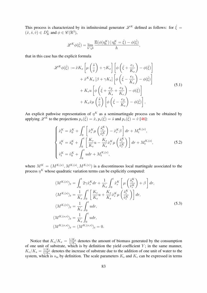
This process is characterized by its infinitesimal generator L K defined as follows: for ξ =(x, s, v) ∈ D3

K and φ ∈ C (R3),

L Kφ(ξ) = limh0

E(φ(ηKh ) | ηK0 = ξ)− φ(ξ)

h,

that in this case has the explicit formula

L Kφ(ξ) := xKx

[µ

(s

v

)+ γKx

] [φ

(ξ +

e1

Kx

)− φ(ξ)

]+ xKKx [β + γKx]

[φ

(ξ − e1

Kx

)− φ(ξ)

]+Kvu

[φ

(ξ +

e2

Ks

+e3

Kv

)− φ(ξ)

]+Kxxµ

(s

v

)[φ

(ξ − e2

Ks

)− φ(ξ)

],

(5.1)

An explicit pathwise representation of ηK as a semimartingale process can be obtained byapplying L K to the projections px(ξ) = x, ps(ξ) = s and pv(ξ) = v [46]:

xKt = xK0 +

∫ t

0

[xKr µ

(sKrvKr

)− xKr β

]dr +M

K,(x)t ,

sKt = sK0 +

∫ t

0

[Kv

Ks

u− Kx

Ks

xKr µ

(sKrvKr

)]dr +M

K,(s)t ,

vKt = vK0 +

∫ t

0

udr +MK,(v)t ,

(5.2)

where MK = (MK,(x),MK,(s),MK,(v)) is a discontinuous local martingale associated to theprocess ηK whose quadratic variation terms can be explicitly computed:

〈MK,(x)〉t =

∫ t

0

2γxKr dr +1

Kx

∫ t

0

xKr

[µ

(sKrvKr

)+ β

]dr,

〈MK,(s)〉t =1

Ks

∫ t

0

[Kv

Ks

u+Kx

Ks

xKr µ

(sKrvKr

)]dr,

〈MK,(v)〉t =1

Kv

∫ t

0

udr,

〈MK,(s,v)〉t =1

Ks

∫ t

0

udr,

〈MK,(x,s)〉t = 〈MK,(x,v)〉t = 0.

(5.3)

Notice that Ks/Kx = 1/Kx1/Ks

denotes the amount of biomass generated by the consumptionof one unit of substrate, which is by definition the yield coefficient Y ; in the same manner,Kv/Ks = 1/Ks

1/Kvdenotes the increase of substrate due to the addition of one unit of water to the

system, which is sin by definition. The scale parameters Ks and Kv can be expressed in terms

83

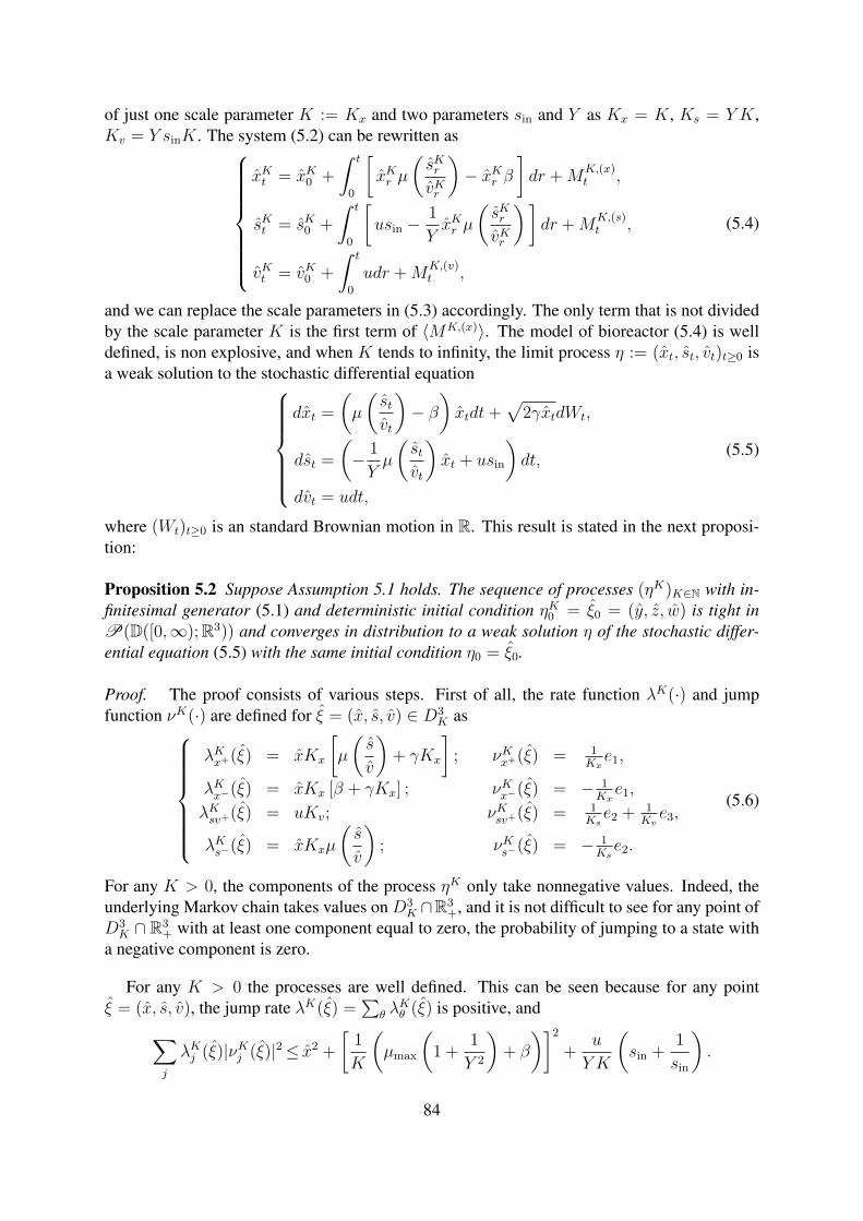
of just one scale parameter K := Kx and two parameters sin and Y as Kx = K, Ks = Y K,Kv = Y sinK. The system (5.2) can be rewritten as

xKt = xK0 +

∫ t

0

[xKr µ

(sKrvKr

)− xKr β

]dr +M

K,(x)t ,

sKt = sK0 +

∫ t

0

[usin −

1

YxKr µ

(sKrvKr

)]dr +M

K,(s)t ,

vKt = vK0 +

∫ t

0

udr +MK,(v)t ,

(5.4)

and we can replace the scale parameters in (5.3) accordingly. The only term that is not dividedby the scale parameter K is the first term of 〈MK,(x)〉. The model of bioreactor (5.4) is welldefined, is non explosive, and when K tends to infinity, the limit process η := (xt, st, vt)t≥0 isa weak solution to the stochastic differential equation

dxt =

(µ

(stvt

)− β

)xtdt+

√2γxtdWt,

dst =

(− 1

Yµ

(stvt

)xt + usin

)dt,

dvt = udt,

(5.5)

where (Wt)t≥0 is an standard Brownian motion in R. This result is stated in the next proposi-tion:

Proposition 5.2 Suppose Assumption 5.1 holds. The sequence of processes (ηK)K∈N with in-finitesimal generator (5.1) and deterministic initial condition ηK0 = ξ0 = (y, z, w) is tight inP(D([0,∞);R3)) and converges in distribution to a weak solution η of the stochastic differ-ential equation (5.5) with the same initial condition η0 = ξ0.

Proof. The proof consists of various steps. First of all, the rate function λK(·) and jumpfunction νK(·) are defined for ξ = (x, s, v) ∈ D3

K as

λKx+(ξ) = xKx

[µ

(s

v

)+ γKx

]; νKx+(ξ) = 1

Kxe1,

λKx−(ξ) = xKx [β + γKx] ; νKx−(ξ) = − 1Kxe1,

λKsv+(ξ) = uKv; νKsv+(ξ) = 1Kse2 + 1

Kve3,

λKs−(ξ) = xKxµ

(s

v

); νKs−(ξ) = − 1

Kse2.

(5.6)

For any K > 0, the components of the process ηK only take nonnegative values. Indeed, theunderlying Markov chain takes values on D3

K ∩R3+, and it is not difficult to see for any point of

D3K ∩ R3

+ with at least one component equal to zero, the probability of jumping to a state witha negative component is zero.

For any K > 0 the processes are well defined. This can be seen because for any pointξ = (x, s, v), the jump rate λK(ξ) =

∑θ λ

Kθ (ξ) is positive, and∑

j

λKj (ξ)|νKj (ξ)|2≤ x2 +

[1

K

(µmax

(1 +

1

Y 2

)+ β

)]2

+u

Y K

(sin +

1

sin

).

84

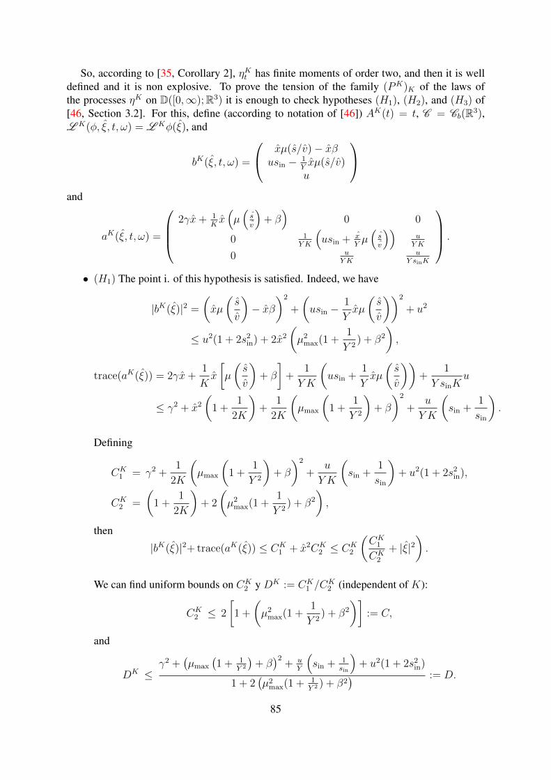
So, according to [35, Corollary 2], ηKt has finite moments of order two, and then it is welldefined and it is non explosive. To prove the tension of the family (PK)K of the laws ofthe processes ηK on D([0,∞);R3) it is enough to check hypotheses (H1), (H2), and (H3) of[46, Section 3.2]. For this, define (according to notation of [46]) AK(t) = t, C = Cb(R3),L K(φ, ξ, t, ω) = L Kφ(ξ), and

bK(ξ, t, ω) =

xµ(s/v)− xβusin − 1

Yxµ(s/v)u

and

aK(ξ, t, ω) =

2γx+ 1

Kx(µ(sv

)+ β

)0 0

0 1Y K

(usin + x

Yµ(sv

))uY K

0 uY K

uY sinK

.

• (H1) The point i. of this hypothesis is satisfied. Indeed, we have

|bK(ξ)|2 =

(xµ

(s

v

)− xβ

)2

+

(usin −

1

Yxµ

(s

v

))2

+ u2

≤ u2(1 + 2s2in) + 2x2

(µ2

max(1 +1

Y 2) + β2

),

trace(aK(ξ)) = 2γx+1

Kx

[µ

(s

v

)+ β

]+

1

Y K

(usin +

1

Yxµ

(s

v

))+

1

Y sinKu

≤ γ2 + x2

(1 +

1

2K

)+

1

2K

(µmax

(1 +

1

Y 2

)+ β

)2

+u

Y K

(sin +

1

sin

).

Defining

CK1 = γ2 +

1

2K

(µmax

(1 +

1

Y 2

)+ β

)2

+u

Y K

(sin +

1

sin

)+ u2(1 + 2s2

in),

CK2 =

(1 +

1

2K

)+ 2

(µ2

max(1 +1

Y 2) + β2

),

then

|bK(ξ)|2+ trace(aK(ξ)) ≤ CK1 + x2CK

2 ≤ CK2

(CK

1

CK2

+ |ξ|2).

We can find uniform bounds on CK2 y DK := CK

1 /CK2 (independent of K):

CK2 ≤ 2

[1 +

(µ2

max(1 +1

Y 2) + β2

)]:= C,

and

DK ≤γ2 +

(µmax

(1 + 1

Y 2

)+ β

)2+ u

Y

(sin + 1

sin

)+ u2(1 + 2s2

in)

1 + 2(µ2

max(1 + 1Y 2 ) + β2

) := D.

85

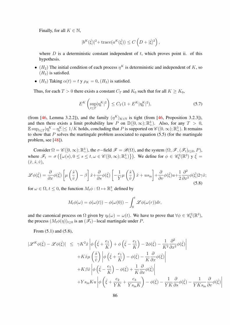
Finally, for all K ∈ N,

|bK(ξ)|2+ trace(aK(ξ)) ≤ C(D + |ξ|2

),

where D is a deterministic constant independent of t, which proves point ii. of thishypothesis.

• (H2) The initial condition of each process ηK is deterministic and independent of K, so(H2) is satisfied.

• (H3) Taking α(t) = t y ρK = 0, (H3) is satisfied.

Thus, for each T > 0 there exists a constant CT and K0 such that for all K ≥ K0,

EK

(supt≤T|ηKt |2

)≤ CT (1 + EK |ηK0 |2), (5.7)

(from [46, Lemma 3.2.2]), and the family (ηK)K∈N is tight (from [46, Proposition 3.2.3]),and then there exists a limit probability law P on D([0,∞);R3

+). Also, for any T > 0,E supt≤T |ηKt −ηKt−|≤ 1/K holds, concluding that P is supported on C ([0,∞);R3

+). It remainsto show that P solves the martingale problem associated to equation (5.5) (for the martingaleproblem, see [48]).

Consider Ω = C ([0,∞);R3+), the σ−field F = B(Ω), and the system (Ω,F , (Ft)t≥0, P ),

where Ft = σ(ω(s), 0 ≤ s ≤ t, ω ∈ C ([0,∞);R3

+))

. We define for φ ∈ C 2b (R3) y ξ =

(x, s, v),

L φ(ξ) =∂

∂xφ(ξ)

[µ

(s

v

)− β

]x+

∂

∂sφ(ξ)

[− 1

Yµ

(s

v

)x+ usin

]+∂

∂vφ(ξ)u+

1

2

∂2

∂x2φ(ξ)2γx;

(5.8)for ω ∈ Ω, t ≤ 0, the function Mtφ : Ω 7→ R3

+ defined by

Mtφ(ω) = φ(ω(t))− φ(ω(0))−∫ t

0

L φ(ω(r))dr,

and the canonical process on Ω given by ηt(ω) = ω(t). We have to prove that ∀φ ∈ C 2b (R3),

the process (Mtφ(η))t≥0 is an (Ft)−local martingale under P .

From (5.1) and (5.8),

|L Kφ(ξ)−L φ(ξ)| ≤ γK2x

∣∣∣∣φ(ξ +e1

K

)+ φ

(ξ − e1

K

)− 2φ(ξ)− 1

K2

∂2

∂x2φ(ξ)

∣∣∣∣+Kxµ

(s

v

) ∣∣∣∣φ(ξ +e1

K

)− φ(ξ)− 1

K

∂

∂xφ(ξ)

∣∣∣∣+Kβx

∣∣∣∣φ(ξ − e1

K

)− φ(ξ) +

1

K

∂

∂xφ(ξ)

∣∣∣∣+Y sinKu

∣∣∣∣φ(ξ +e2

Y K+

e3

Y sinK

)− φ(ξ)− 1

Y K

∂

∂sφ(ξ)− 1

Y Ksin

∂

∂vφ(ξ)

∣∣∣∣86

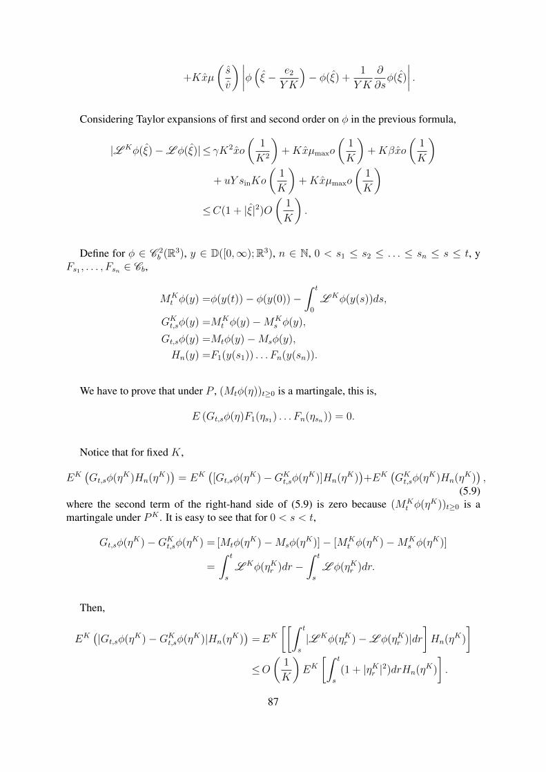
+Kxµ

(s

v

) ∣∣∣∣φ(ξ − e2

Y K

)− φ(ξ) +

1

Y K

∂

∂sφ(ξ)

∣∣∣∣ .Considering Taylor expansions of first and second order on φ in the previous formula,

|L Kφ(ξ)−L φ(ξ)| ≤ γK2xo

(1

K2

)+Kxµmaxo

(1

K

)+Kβxo

(1

K

)+ uY sinKo

(1

K

)+Kxµmaxo

(1

K

)≤C(1 + |ξ|2)O

(1

K

).

Define for φ ∈ C 2b (R3), y ∈ D([0,∞);R3), n ∈ N, 0 < s1 ≤ s2 ≤ . . . ≤ sn ≤ s ≤ t, y

Fs1 , . . . , Fsn ∈ Cb,

MKt φ(y) =φ(y(t))− φ(y(0))−

∫ t

0

L Kφ(y(s))ds,

GKt,sφ(y) =MK

t φ(y)−MKs φ(y),

Gt,sφ(y) =Mtφ(y)−Msφ(y),

Hn(y) =F1(y(s1)) . . . Fn(y(sn)).

We have to prove that under P , (Mtφ(η))t≥0 is a martingale, this is,

E (Gt,sφ(η)F1(ηs1) . . . Fn(ηsn)) = 0.

Notice that for fixed K,

EK(Gt,sφ(ηK)Hn(ηK)

)= EK

([Gt,sφ(ηK)−GK

t,sφ(ηK)]Hn(ηK))+EK

(GKt,sφ(ηK)Hn(ηK)

),

(5.9)where the second term of the right-hand side of (5.9) is zero because (MK

t φ(ηK))t≥0 is amartingale under PK . It is easy to see that for 0 < s < t,

Gt,sφ(ηK)−GKt,sφ(ηK) = [Mtφ(ηK)−Msφ(ηK)]− [MK

t φ(ηK)−MKs φ(ηK)]

=

∫ t

s

L Kφ(ηKr )dr −∫ t

s

L φ(ηKr )dr.

Then,

EK(|Gt,sφ(ηK)−GK

t,sφ(ηK)|Hn(ηK))

=EK

[[∫ t

s

|L Kφ(ηKr )−L φ(ηKr )|dr]Hn(ηK)

]≤O

(1

K

)EK

[∫ t

s

(1 + |ηKr |2)drHn(ηK)

].

87

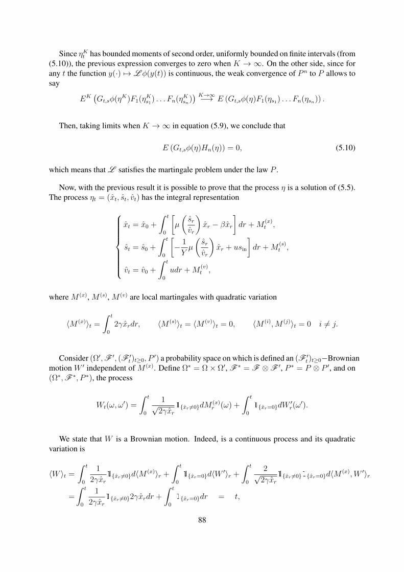
Since ηKt has bounded moments of second order, uniformly bounded on finite intervals (from(5.10)), the previous expression converges to zero when K → ∞. On the other side, since forany t the function y(·) 7→ L φ(y(t)) is continuous, the weak convergence of P n to P allows tosay

EK(Gt,sφ(ηK)F1(ηKs1) . . . Fn(ηKsn)

) K→∞−→ E (Gt,sφ(η)F1(ηs1) . . . Fn(ηsn)) .

Then, taking limits when K →∞ in equation (5.9), we conclude that

E (Gt,sφ(η)Hn(η)) = 0, (5.10)

which means that L satisfies the martingale problem under the law P .

Now, with the previous result it is possible to prove that the process η is a solution of (5.5).The process ηt = (xt, st, vt) has the integral representation

xt = x0 +

∫ t

0

[µ

(srvr

)xr − βxr

]dr +M

(x)t ,

st = s0 +

∫ t

0

[− 1

Yµ

(srvr

)xr + usin

]dr +M

(s)t ,

vt = v0 +

∫ t

0

udr +M(v)t ,

where M (x), M (s), M (v) are local martingales with quadratic variation

〈M (x)〉t =

∫ t

0

2γxrdr, 〈M (s)〉t = 〈M (v)〉t = 0, 〈M (i),M (j)〉t = 0 i 6= j.

Consider (Ω′,F ′, (F ′t )t≥0, P

′) a probability space on which is defined an (F ′t )t≥0−Brownian

motion W ′ independent of M (x). Define Ω∗ = Ω× Ω′, F ∗ = F ⊗F ′, P ∗ = P ⊗ P ′, and on(Ω∗,F ∗, P ∗), the process

Wt(ω, ω′) =

∫ t

0

1√2γxr

1xr 6=0dM(x)r (ω) +

∫ t

0

1xr=0dW′r(ω′).

We state that W is a Brownian motion. Indeed, is a continuous process and its quadraticvariation is

〈W 〉t =

∫ t

0

1

2γxr1xr 6=0d〈M (x)〉r +

∫ t

0

1xr=0d〈W ′〉r +

∫ t

0

2√2γxr

1xr 6=01xr=0d〈M (x),W ′〉r

=

∫ t

0

1

2γxr1xr 6=02γxrdr +

∫ t

0

1xr=0dr = t,

88

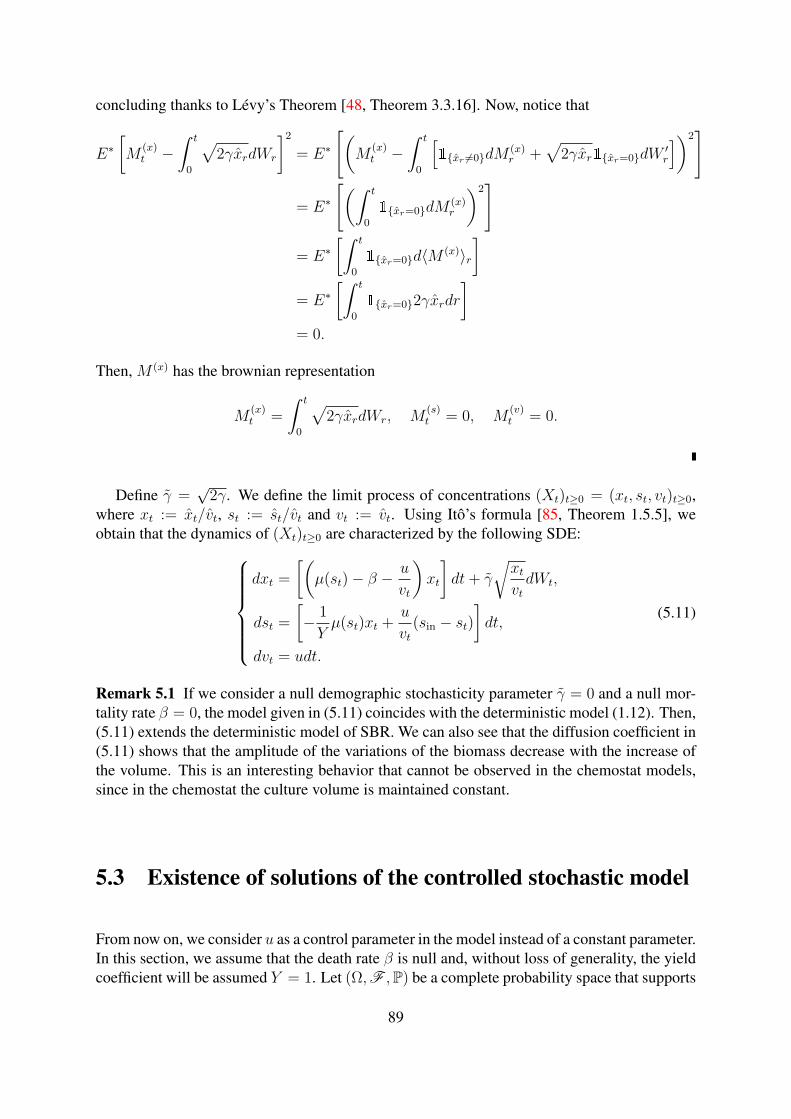
concluding thanks to Lévy’s Theorem [48, Theorem 3.3.16]. Now, notice that

E∗[M

(x)t −

∫ t

0

√2γxrdWr

]2

= E∗

[(M

(x)t −

∫ t

0

[1xr 6=0dM

(x)r +

√2γxr1xr=0dW

′r

])2]

= E∗

[(∫ t

0

1xr=0dM(x)r

)2]

= E∗[∫ t

0

1xr=0d〈M (x)〉r]

= E∗[∫ t

0

1xr=02γxrdr

]= 0.

Then, M (x) has the brownian representation

M(x)t =

∫ t

0

√2γxrdWr, M

(s)t = 0, M

(v)t = 0.

Define γ =√

2γ. We define the limit process of concentrations (Xt)t≥0 = (xt, st, vt)t≥0,where xt := xt/vt, st := st/vt and vt := vt. Using Itô’s formula [85, Theorem 1.5.5], weobtain that the dynamics of (Xt)t≥0 are characterized by the following SDE:

dxt =

[(µ(st)− β −

u

vt

)xt

]dt+ γ

√xtvtdWt,

dst =

[− 1

Yµ(st)xt +

u

vt(sin − st)

]dt,

dvt = udt.

(5.11)

Remark 5.1 If we consider a null demographic stochasticity parameter γ = 0 and a null mor-tality rate β = 0, the model given in (5.11) coincides with the deterministic model (1.12). Then,(5.11) extends the deterministic model of SBR. We can also see that the diffusion coefficient in(5.11) shows that the amplitude of the variations of the biomass decrease with the increase ofthe volume. This is an interesting behavior that cannot be observed in the chemostat models,since in the chemostat the culture volume is maintained constant.

5.3 Existence of solutions of the controlled stochastic model

From now on, we consider u as a control parameter in the model instead of a constant parameter.In this section, we assume that the death rate β is null and, without loss of generality, the yieldcoefficient will be assumed Y = 1. Let (Ω,F ,P) be a complete probability space that supports

89

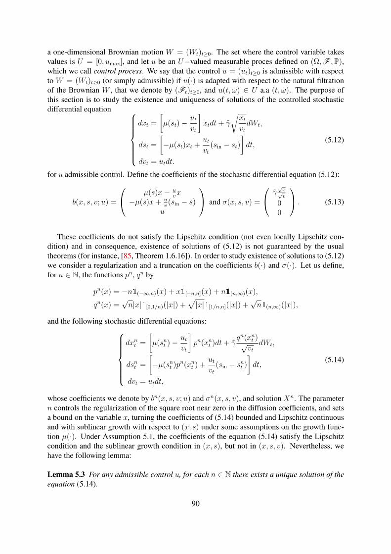
a one-dimensional Brownian motion W = (Wt)t≥0. The set where the control variable takesvalues is U = [0, umax], and let u be an U−valued measurable proces defined on (Ω,F ,P),which we call control process. We say that the control u = (ut)t≥0 is admissible with respectto W = (Wt)t≥0 (or simply admissible) if u(·) is adapted with respect to the natural filtrationof the Brownian W , that we denote by (Ft)t≥0, and u(t, ω) ∈ U a.a (t, ω). The purpose ofthis section is to study the existence and uniqueness of solutions of the controlled stochasticdifferential equation

dxt =

[µ(st)−

utvt

]xtdt+ γ

√xtvtdWt,

dst =

[−µ(st)xt +

utvt

(sin − st)]dt,

dvt = utdt.

(5.12)

for u admissible control. Define the coefficients of the stochastic differential equation (5.12):

b(x, s, v;u) =

µ(s)x− uvx

−µ(s)x+ uv(sin − s)

u

and σ(x, s, v) =

γ√x√v

00

. (5.13)

These coefficients do not satisfy the Lipschitz condition (not even locally Lipschitz con-dition) and in consequence, existence of solutions of (5.12) is not guaranteed by the usualtheorems (for instance, [85, Theorem 1.6.16]). In order to study existence of solutions to (5.12)we consider a regularization and a truncation on the coefficients b(·) and σ(·). Let us define,for n ∈ N, the functions pn, qn by

pn(x) = −n1(−∞,n)(x) + x1[−n,n](x) + n1(n,∞)(x),

qn(x) =√n|x|1[0,1/n)(|x|) +

√|x|1[1/n,n](|x|) +

√n1(n,∞)(|x|),

and the following stochastic differential equations:dxnt =

[µ(snt )− ut

vt

]pn(xnt )dt+ γ

qn(xnt )√vt

dWt,

dsnt =

[−µ(snt )pn(xnt ) +

utvt

(sin − snt )

]dt,

dvt = utdt,

(5.14)

whose coefficients we denote by bn(x, s, v;u) and σn(x, s, v), and solution Xn. The parametern controls the regularization of the square root near zero in the diffusion coefficients, and setsa bound on the variable x, turning the coefficients of (5.14) bounded and Lipschitz continuousand with sublinear growth with respect to (x, s) under some assumptions on the growth func-tion µ(·). Under Assumption 5.1, the coefficients of the equation (5.14) satisfy the Lipschitzcondition and the sublinear growth condition in (x, s), but not in (x, s, v). Nevertheless, wehave the following lemma:

Lemma 5.3 For any admissible control u, for each n ∈ N there exists a unique solution of theequation (5.14).

90

Proof. Given u = (ut)t≥0 admissible control, the volume process v = (vt)t≥0 has the explicitrepresentation

vt(ω) = w +

∫ t

0

ur(ω)dr. (5.15)

Define the process Xn = (xnt , snt )t≥0 as the solution of the following stochastic differential

equation with random coefficients bn(t, x, s;ω) and σn(t, x, s;ω) given bydxnt =

[µ(snt )− ut

vt(ω)

]pn(xnt )dt+ γ

qn(xnt )√vt(ω)

dWt,

dsnt =

[−µ(snt )pn(xnt ) +

utvt

(ω)(sin − snt )

]dt.

(5.16)

We notice that given the control u(·), for each (x, s) ∈ R2, t ≥ 0, and ω ∈ Ω,

bn(x, s, vt(ω);ut(ω)) =

(bn(t, x, s;ω)

vt(ω)

), σn(x, s, vt(ω)) =

(σn(t, x, s;ω)

0

), (5.17)

hence, on (Ω,F , (Ft)t≥0,P), with control u, Brownian motion W , and initial condition ξ0,the solutions of (5.14) and (5.16) are the same. The coefficients bn(·) and σn(·) are Lipschitzcontinuous in (x, s) and have sublinear growth in (x, s), uniformly in t:

|b(t, x, s, ω)− b(t, x′, s′, ω)| ≤(µmax +

umax

vmin

)|x− x′|+nLµ|s− s′|,

|σ(t, x, s, ω)− σ(t, x′, s′, ω)| ≤ γ√vt(ω)

|qn(x)− qn(x′)|≤ γ√vmin

|x− x′|,

where Lµ is the Lipschitz constant of µ, and

b(t, x, s, ω) ≤(

2µmax +umax

vmin

)x+

umax

vmin

s+umax

vmin

sin,

σ(t, x, s, ω) ≤ γ√vmin

(1 + |x|).

Consequently, according to [85, Theorem 1.6.16], for all n ∈ N the equation (5.16) has aunique solution; then, for all n ∈ N, equation (5.14) has a controlled solution Xn = (Xn

t )t≥0.

Let us define for each n ∈ N the stopping time τn := inft > 0 | |xnt |> n ∨ |xnt |< 1/n,which is the first time when the dynamics (5.14) are truncated, and τ := supn∈N τ

n. Thestopping time τ is well defined, because it is the limit of a sequence of increasing stoppingtimes, and thanks to the pathwise uniqueness, for m > n it is not difficult to see that Xm

t = Xnt

in the set t ≤ τn.

Lemma 5.4 The process Zn·∧τn = (Zn

t∧τn)t≥0, where Znt is defined by

Znt = (xnt + snt − sin)vt, (5.18)

is a continuous local martingale with respect to (Ft)t≥0.

91

Proof. Using Itô’s formula for Zn, we get

Znt = Zn

0 +

∫ t

0

[xnr − pn(xnr )]urdr +

∫ t

0

γqn(xnr )√vrdWr,

with Zn0 = (xn0 + sn0 − sin)v0 = (y + z − sin)w. In the set r ≤ τn we have pn(xnr ) = xnr and

qn(xnr ) =√xnr ; then, we can write

Znt∧τn = Zn

0 + γ

∫ t∧τn

0

√xnr vrdWr, (5.19)

from which the result follows.

Lemma 5.5 For all T ≥ 0, we have

supn>0

E[supt≤T|Xn

t∧τn|]<∞.

Proof. We analyze, as a first step, the behavior of snt . The process snt has paths of finitevariation, so it can be studied in terms of its infinitesimal variations. It is non-negative, becauseif at some time instant t > 0 we have snt = 0, the equation of sn reads

dsnt =utvtsindt ≥ 0,

so sn will be increasing. The process snt is also bounded. Indeed, thanks to pathwise unique-ness, xnt is always nonnegative. If at some time instant t ≥ 0 we have that snt ≥ sin, then

dsnt =

[−µ(snt )pn(xnt ) +

utvt

(sin − snt )

]dt ≤ 0,

so snt will be decreasing. Now, consider the process Zn defined by (5.18). Thanks to (5.19), wecan write

[xnt∧τn + snt∧τn − sin] vt∧τn = [y + z − sin]w +

∫ t∧τn

0

γ√xnr vrdWr. (5.20)

The process sn = (snt )t≥0 is always non-negative, and (vt)t≥0 is non-decreasing and boundedfrom above by vmax, so

xnt v0 = xnt vt + snt vt − sinvt + sinvt

≤ [xnt + snt − sin] vt + sinvmax.(5.21)

Replacing (5.20) in (5.21), with v0 = w,

xnt∧τnw ≤ [y + z − sin]w + sinvmax +

∫ t∧τn

0

γ√xnr vrdWr.

92

Define κ := [y + z − sin]w + sinvmax. Taking supremum on [0, T ] and expectation,

E[w sup

t≤Txnt∧τn

]≤ κ+ E

[supt≤T

∫ t∧τn

0

γ√xnr vrdWr

].

Using the Burkholder-Davis-Gundy inequality [48, Theorem 3.3.28], we obtain the exis-tence of a constant C > 0 independent of n such that

E[supt≤T

∫ t∧τn

0

γ√xnr vrdWr

]≤ CE

[(∫ T∧τn

0

γ2xnr vrdr

) 12

],

hence

E[supt≤T

xnt∧τn

]≤ κ

w+

1

wCE

[(∫ T∧τn

0

γ2xnr vrdr

) 12

]

≤ 1

wκ+

1

wCγE

[1 +

∫ T∧τn

0

xnr vrdr

]≤ 1

w[κ+ Cγ] + γC

vmax

wE[∫ T

0

supr′≤r

xnr′∧τndr

].

Using Gronwall’s inequality [48, Problem 5.2.7], and taking supremum over n > 0, weconclude that

supn>0

E[supt≤T

xnt∧τn

]<∞.

We define the process X = (x, s, v) in the following way: for n ≥ 1, n ∈ N,

Xt = Xnt , in the set t ≤ τn.

It is easy to see that P−a.s., for all t ≥ 0,

Xt∧τn = ξ +

∫ t∧τn

0

b(Xr, ur)dr +

∫ t∧τn

0

σ(Xr)dWr, (5.22)

where b(·) and σ(·) are the coefficients defined in (5.13). The process X is defined up to thefinal time τ , and then, equation (5.12) in its integral form (5.22) has a solution defined in thetime interval [0, τ ]. It remains to prove that τ is the first time that xt reaches 0 (possibly infinite).

Proposition 5.6 P−almost surely, τ = τE := inft ≥ 0 : xt = 0.

Proof. Suppose that P(τ 6= τE) > 0, and define A = ω ∈ Ω | τ(ω) 6= τE(ω). Notice that ifτ = ∞, then τE = ∞, so necessarily A ⊆ τ < ∞. Then, for almost all ω ∈ A there existsan increasing sequence (nk(ω))k∈N ∞ such that xτnk(ω)(ω) = nk(ω)∞.

93

Notice that there must exist a T > 0 such that P(A ∩ τ ≤ T) > 0. Indeed, if such Tdoes not exist, for every N ∈ N we have P(A ∩ τ ≤ N) = 0. Notice that the sequenceof sets A ∩ τ ≤ N is increasing with N and converges to A ∩ τ < ∞, concluding thatP(A ∩ τ <∞) = 0, which contradicts the initial assumption.

Now, consider the T such that P(A∩ τ ≤ T) > 0. For almost each ω ∈ A∩ τ ≤ T wehave that supt∈[0,T ] xt∧τnk (ω)(ω) = nk(ω), and then

supn∈N

E

[supt∈[0,T ]

xt∧τn

]≥ sup

k∈NE

[supt∈[0,T ]

xt∧τnk (ω)(ω)1A∩τ≤T

]=∞,

which contradicts Lemma 5.5.

The last proposition shows that the equation (5.12) has a solution up to τ , and that pathwiseuniqueness holds. Now, we present a result that shows the behavior of the process with respectto extinction of the biomass. In the deterministic case the extinction time is infinite unlessthe initial condition is such that x(0) = 0, but in the stochastic framework the possibility ofextinction must be considered (see [15, 41]). This is a serious issue in terms of the depollu-tion process, because extinction of the biomass before reaching the target stops the treatment,making it impossible to reach the target without considering other types of strategies such asadding biomass to the system when a critical level is reached. For equation (5.12), we have thefollowing result:

Proposition 5.7 Let u = (ut)t≥0 be an admissible control with respect to W = (Wt)t≥0 andXu = (xu, su, vu) the solution of (5.12). The probability that xu = (xut )t≥0 hits 0 at some timeinstant is positive.

Proof. Consider the continuous local martingale

Mut =

∫ t∧τ

0

1√vurdWr,

whose quadratic variation is

〈Mu〉t =

∫ t∧τ

0

1

vurdr.

Since (vut )t≥0 es positive, non-decreasing and bounded up to τ , then S := limt→∞〈Mu〉t =∫ τ0

1vurdr, P− a.s. Let us define, for r ∈ [0,∞), the stopping time

T (r) =

inft ≥ 0 | 〈Mu〉t > r, r < S,

∞, r ≥ S.

According to [40, Theorem II.7.2’], defining Br = MuT (r), Gr = FT (r), it is possible to con-

struct an extension of (Ω,F , (Ft)t≥0,P), namely (Ω, F , (Ft), P) on which there is a Brownianmotion B′ independent of (Nr,Gr) such that the process

Br = Br +B′r −B′r∧S

94

is a standard unidimensional Brownian motion defined in (Ω, F , (Ft), P). Then, Xu (thesolution of (5.12)) can be written in terms of the new time r and new Brownian motion (Br)r≥0

(in (Ω, F , (Ft), P)) as follows: renaming xr = xT (r), sr = sT (r), vr = vT (r) and ur = uT (r),X u = (xu, su, vu) solves

dxr = [µ(sr)vr − ur] xrdr + γ√xrdBr,

dsr = [−µ(sr)vrxr + ur(sin − sr)] dr,dvr = urvrdr,

(5.23)

with initial condition ξ = (y, z, w), for 0 ≤ r ≤ S (the process is stopped at r = S). We noticethat

Pξ (∃t ∈ [0,∞) : xut = 0) = Pξ(∃r ∈ [0,∞) : xur = 0

).

Now, consider the process x = (xr)r≥0 defined as the solution of

dxr = µmaxvmaxxrdr + γ√xrdBr, x0 = y. (5.24)

Strong existence and pathwise uniqueness hold for the equation (5.24) (from [52, Theorem 6.2.3]),and it is defined for r ∈ [0,∞). Since µ(·) is bounded, then for any r ≥ 0, µ(sr) ≤ µmax andvr ≤ vmax. Then, thanks to comparison principles (for instance, see [40, Theorem VI.1.1], withβ

(1)r = (µ(sr)vr − ur)xr, β(2)

r = µmaxvmaxxr, b1(r, x) = b2(r, x) = µmaxvmaxx), we get

Pξ(xur ≤ xr, ∀r ∈ [0,∞)

)= 1.

Comparing the CIR model in [52, Proposition 6.2.4] and (5.24) (with a = 0, b = −µmaxvmax

y σ = γ), the probability that x hits zero belongs to (0, 1). We conclude then

Pξ (∃t ∈ [0,∞) : xut = 0) = Pξ(∃r ∈ [0,∞) : xur = 0

)≥ Py (∃r ∈ [0,∞) : xr = 0)

> 0.

Thus, the probability of extinction of biomass is positive.

5.4 The optimal reach-avoid problem

Consider the domainD := [0,∞)×[0, sin]×[vmin, vmax], the target set C := (0,∞)×[0, sout]×vmax, the full tank set V := (0,∞)×[sout, sin]×vmax, the extinction set E := 0×[0, sin]×[vmin, vmax], and an initial condition ξ ∈ D. Consider a probability space (Ω,F ,P) on which a

95

one-dimensional Brownian motionW = (Wt)t≥0 is defined, and consider the Brownian naturalfiltration F := (Ft)t≥0. We define the set of admissible controls

U = u : [0,∞)× Ω→ [0, umax] | u is F− progresively measurable ,

and denote Xξ,u the solution of the controlled stochastic differential equation (5.12) with con-trol u ∈ U and initial condition ξ. This process takes values on the set D. For a Borelmeasurable set A ⊆ R3 define the hitting times τuA = inf t ≥ 0 |Xu

t ∈ A. Consider, forξ ∈ D and u ∈ U , the cost functional given by the probability of reaching the target set beforeextinction of the biomass:

J(ξ;u) := Pξ [τuC ≤ τuE ] , (5.25)

and the value function(P) V (ξ) := sup

u∈UJ(ξ;u). (5.26)

Remark 5.2 Notice that the value function is bounded between 0 and 1 since it is definedas the supremum of probabilities of events, and it is discontinuous at the boundary of thedomain. Indeed, for ξ ∈ C the value function takes the value V (ξ) = 1, for ξ ∈ E we haveV (ξ) = 0, and cl(C) ∩ E 6= φ. The problem is that the reach set C and the avoid set E cannotbe separated by nonintersecting open sets. The fact that the control on the set V is forced totake the value 0 poses another problem with respect to the standard formulation of the problemas a reach-avoid problem, since we have a state constraint. Nevertheless, for initial conditionsξ0 = (x0, s0, vmax) in the set V it is possible to explicitly compute the probability of hitting thetarget before extinction.

Indeed, in the set V the constraints of the problem impose u ≡ 0, and then the processsatisfies the SDE dxt = µ(st)xtdt+

γ√vmax

√xtdWt, t ∈ [0, τE ∧ τC],

dst = −µ(st)xtdt,

(5.27)

Notice that t 7→ st is decreasing up to τE ∧ τC P−a.s., thus we can define the time-changefunctions

θt := s0 − st =

∫ t

0

µ(sr)xrdr, Tr := inft ≥ 0 : θt > r,

(that depend of (x0, s0)) where the new time will be denoted by r. Denoting xr = xTr ,Wr = N

(1)Tr

, with N(1)t =

∫ t0

õ(sr)xrdWr, the law of this process satisfies the following

SDE independent of st:

dxr = dr +γ

√vmax

1√µ(s0 − r)

dWr, x0 = x0. (5.28)

for r ∈ [0, θτ ], with θτ = θτC ∧ θτE . In this new time scale, in the event τC < τE the time tothe target is θτC = s0 − sout (constant, depending only of s0), and the time to extinction is θτE .The coefficient that accompanies the brownian part in equation (5.28) does not explode, andthis equation provides an explicit expression for xr:

xr = x0 + r ∧ θτE ∧ (s0 − sout) +γ

√vmax

∫ r∧θτE∧(s0−sout)

0

1√µ(s0 − h)

dWh.

96

We make another time-change (that depends of s0) in order to absorb the diffusion coeffi-cient in (5.28). Define

ϕs0r = ϕr :=γ2

vmax

∫ r

0

1

µ(s0 − h)dh, T s0h = Th := infr ≥ 0 : ϕr > h,

In the time h, defining xh = xTh and Wh = N(2)

Th, with N (2)

r = γ√vmax

∫ r0

1√µ(s0−h)

dWh, xhsolves

dxh =vmax

γ2µ(s0 − Th)dh+ dWh, x0 = x0. (5.29)

for h ∈ [0, ϕθτ ]. Define for simplicity, T s0 = T := ϕs0θC , TE = ϕs0θτE. Notice that in the set

τC < τE we have T s0 = ϕs0−sout . Define also As0h = Ah := vmax

γ2

∫ h0µ(s0 − Tα)dα. For

a process M denote M?t = maxs∈[0,t] Ms. In these terms, hitting the target before extinction

corresponds to the event TE > T, xT > 0.Pξ0 [τC < τE ] = P

[TE > T, xT > 0

]= P

[minh∈[0,T ]

x0 + Ah + Wh > 0, TE > T

]= P

[minh∈[0,T ]

Ah + Wh > −x0

].

Consider the probability law Q under which the process Wh−Ah is an Fh-Brownian motion(where Fh = FTTh

), which has density with respect to P given by

Mh = exp

vmax

γ2

∫ h

0

µ(s0 − Tα)dWα −1

2

v2max

γ4

∫ h

0

µ(s0 − Tα)2dα

.

Then,

Pξ0 [τC < τE ] = P[∀h ∈ [0, T ], Wh > −x0 − Ah

]= Q

[∀h ∈ [0, T ], Wh − Ah > −x0 − Ah

]= EQ

[1min

h∈[0,T ]Wh>−x0

]= E

[1min

h∈[0,T ]Wh>−x0MT

]= E

[1min

h∈[0,T ]Wh>−x0 exp

vmax

γ2

∫ T

0

µ(s0 − Tα)dWα −1

2

v2max

γ4

∫ T

0

µ(s0 − Tα)2dα

]

Finally, we get the expression for the cost on V:

Pξ0 [τC < τE ] = exp

−1

2

v2max

γ4

∫ T

0

µ(s0 − Tα)2dα

× E

[1W ?

T<x0 exp

−vmax

γ2

∫ T

0

µ(s0 − Tα)dWα

].

(5.30)

97

Proposition 5.8 The function V 3 ξ 7→ v(ξ) := Pξ [τuC ≤ τuE ] is continuous.

Proof. We study formula (5.30). First, the function s0 7→ ϕs0r is continuous:

|ϕs1r − ϕs2r | ≤1

µ(s1 − r)µ(s2 − r)

∫ r

0

|µ(s1 − h)− µ(s2 − h)|dh

≤ r

µ(s1 − r)µ(s2 − r)maxh∈[0,r]

|µ(s1 − h)− µ(s2 − h)|

Then, s0 7→ T s0r and s0 7→ T s0 = ϕs0s0−soutare continuous, which proves the continuity of the

first term in (5.30). For the continuity of the second term of the right-hand side, define

F (x0, s0) = 1W ?

T<x0

, G(s0) = exp

−vmax

γ2

∫ T s0

0

µ(s0 − T s0α )dWα

.

Then, for ξ = (x, s, vmax) ∈ V ,

E|F (x0, s0)G(s0)− F (x, s)G(s)| ≤E [|F (x0, s0)− F (x, s)|G(s0)]

+ E [F (x, s)|G(s0)−G(s)|]

≤E[|F (x0, s0)− F (x, s)|2

] 12 E[G(s0)2

] 12

+ E [|G(s0)−G(s)|] .

(5.31)

where the last inequality comes from Cauchy-Schwartz inequality and the fact that F (x, s) ≤ 1.Notice that the exponent in the definition of G is a Gaussian variable with null mean andvariance equal to v2

max

γ4

∫ T s00

µ(s0 − T s0α )2dα, so G(s0) is finite (depending on s0). Indeed, withan appropriate change of variables, we can write for any p ≥ 1

E [G(s0)p] = exp

p2

2

vmax

γ2

∫ s0

sout

µ(r)dr

≤ exp

p2

2

vmax

γ2(s0 − sout)µ(s0)

<∞. (5.32)

From the previous expression, we can see that for any s ≤ sin it holds E [G(s)p] ≤ E [G(sin)p] <∞, and we conclude that G(s)s∈[sout,sin] is uniformly integrable. To prove the convergenceof G(s) to G(s0) in L1 when s 7→ s0 it is enough to prove that

∆ :=

∫ T s

0

µ(s− T sα)dWα −∫ T s0

0

µ(s0 − T s0α )dWα → 0 in L2 if s→ s0.

From the Itô isometry, we have

E |∆|2 ≤ 2E

[∫ T s

0

|µ(s− T sα)− µ(s0 − T s0α )|2dα

]+ 2E

[∫ T s

T s0|µ(s0 − T s0α )|2dα

]

≤ 4L2µE

[∫ T s

0

(|s− s0|2+|T sα − T s0α |2)dα

]+ 2µ2

maxE|T s0 − T s|,

(5.33)

98

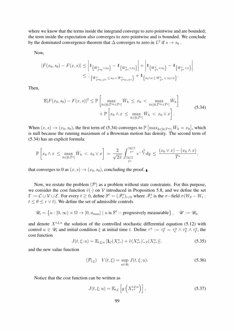
where we know that the terms inside the integrand converge to zero pointwise and are bounded;the term inside the expectation also converges to zero pointwise and is bounded. We concludeby the dominated convergence theorem that ∆ converges to zero in L2 if s→ s0 .

Now,

|F (x0, s0)− F (x, s)| ≤∣∣∣∣1

W ?

Ts0<x0

− 1W ?

Ts<x0

∣∣∣∣+

∣∣∣∣1W ?

Ts<x0

− 1W ?

Ts<x

∣∣∣∣≤ 1

W ?

Ts0∧T s≤x0<W ?

Ts0∨T s

+ 1x0∧x≤ W ?

Ts<x0∨x

.Then,

E|F (x0, s0)− F (x, s)|2 ≤ P[

maxh∈[0,T s0∧T s]

Wh ≤ x0 < maxh∈[0,T s0∨T s]

Wh

]+ P

[x0 ∧ x ≤ max

h∈[0,T s]Wh < x0 ∨ x

].

(5.34)

When (x, s) → (x0, s0), the first term of (5.34) converges to P[maxh∈[0,T s0 ] Wh = x0

], which

is null because the running maximum of a Brownian motion has density. The second term of(5.34) has an explicit formula:

P[x0 ∧ x ≤ max

h∈[0,T s]Wh < x0 ∨ x

]=

2√2π

∫ x0∨x¯Ts

x0∧x¯Ts

e−y2

2 dy ≤ (x0 ∨ x)− (x0 ∧ x)

T s,

that converges to 0 as (x, s)→ (x0, s0), concluding the proof.

Now, we restate the problem (P) as a problem without state constraints. For this purpose,we consider the cost function v(·) on V introduced in Proposition 5.8, and we define the setΓ := C ∪ V ∪ E . For every t ≥ 0, define Ft = (F t

r)r≥0 where F tr is the σ−field σ(Wθ −Wt :

t ≤ θ ≤ r ∨ t). We define the set of admissible controls

Ut =u : [0,∞)× Ω→ [0, umax] | u is Ft − progresively measurable

, U := U0,

and denote X t,ξ,u the solution of the controlled stochastic differential equation (5.12) withcontrol u ∈ Ut and initial condition ξ at initial time t. Define τu := τuΓ = τuC ∧ τuV ∧ τuE , thecost function

J(t, ξ;u) = Et,ξ;u [1C(Xuτu) + v(Xu

τu)1V(Xuτu)] . (5.35)

and the new value function

(Pt,ξ) V (t, ξ) = supu∈Ut

J(t, ξ;u). (5.36)

Notice that the cost function can be written as

J(t, ξ;u) = Et,ξ[g(X t,ξ;uτu

)], (5.37)

99

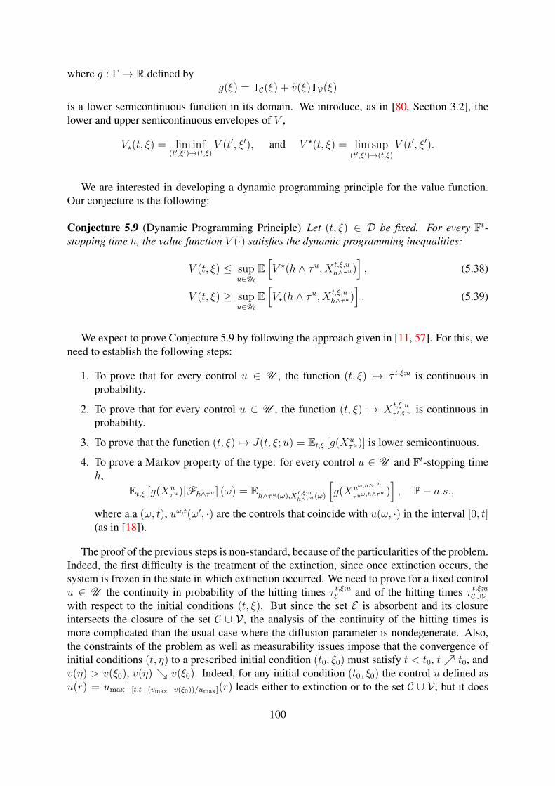
where g : Γ→ R defined byg(ξ) = 1C(ξ) + v(ξ)1V(ξ)

is a lower semicontinuous function in its domain. We introduce, as in [80, Section 3.2], thelower and upper semicontinuous envelopes of V ,

V?(t, ξ) = lim inf(t′,ξ′)→(t,ξ)

V (t′, ξ′), and V ?(t, ξ) = lim sup(t′,ξ′)→(t,ξ)

V (t′, ξ′).

We are interested in developing a dynamic programming principle for the value function.Our conjecture is the following:

Conjecture 5.9 (Dynamic Programming Principle) Let (t, ξ) ∈ D be fixed. For every Ft-stopping time h, the value function V (·) satisfies the dynamic programming inequalities:

V (t, ξ) ≤ supu∈Ut

E[V ?(h ∧ τu, X t,ξ,u

h∧τu)], (5.38)

V (t, ξ) ≥ supu∈Ut

E[V?(h ∧ τu, X t,ξ,u

h∧τu)]. (5.39)

We expect to prove Conjecture 5.9 by following the approach given in [11, 57]. For this, weneed to establish the following steps:

1. To prove that for every control u ∈ U , the function (t, ξ) 7→ τ t,ξ;u is continuous inprobability.

2. To prove that for every control u ∈ U , the function (t, ξ) 7→ X t,ξ;uτ t,ξ,u

is continuous inprobability.

3. To prove that the function (t, ξ) 7→ J(t, ξ;u) = Et,ξ [g(Xuτu)] is lower semicontinuous.

4. To prove a Markov property of the type: for every control u ∈ U and Ft-stopping timeh,

Et,ξ [g(Xuτu)|Fh∧τu ] (ω) = Eh∧τu(ω),Xt,ξ;u

h∧τu (ω)

[g(Xuω,h∧τ

u

τuω,h∧τu )

], P− a.s.,

where a.a (ω, t), uω,t(ω′, ·) are the controls that coincide with u(ω, ·) in the interval [0, t](as in [18]).

The proof of the previous steps is non-standard, because of the particularities of the problem.Indeed, the first difficulty is the treatment of the extinction, since once extinction occurs, thesystem is frozen in the state in which extinction occurred. We need to prove for a fixed controlu ∈ U the continuity in probability of the hitting times τ t,ξ;uE and of the hitting times τ t,ξ;uC∪Vwith respect to the initial conditions (t, ξ). But since the set E is absorbent and its closureintersects the closure of the set C ∪ V , the analysis of the continuity of the hitting times ismore complicated than the usual case where the diffusion parameter is nondegenerate. Also,the constraints of the problem as well as measurability issues impose that the convergence ofinitial conditions (t, η) to a prescribed initial condition (t0, ξ0) must satisfy t < t0, t t0, andv(η) > v(ξ0), v(η) v(ξ0). Indeed, for any initial condition (t0, ξ0) the control u defined asu(r) = umax1[t,t+(vmax−v(ξ0))/umax](r) leads either to extinction or to the set C ∪ V , but it does

100

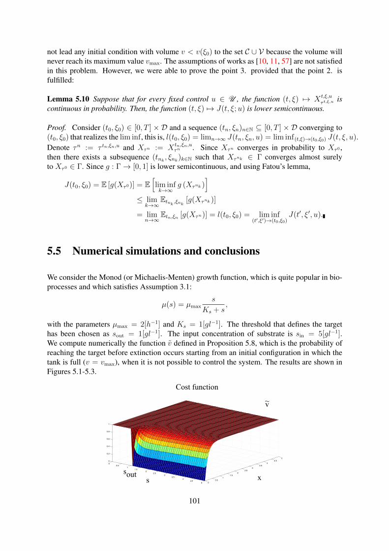
not lead any initial condition with volume v < v(ξ0) to the set C ∪ V because the volume willnever reach its maximum value vmax. The assumptions of works as [10, 11, 57] are not satisfiedin this problem. However, we were able to prove the point 3. provided that the point 2. isfulfilled:

Lemma 5.10 Suppose that for every fixed control u ∈ U , the function (t, ξ) 7→ X t,ξ,uτ t,ξ,u

iscontinuous in probability. Then, the function (t, ξ) 7→ J(t, ξ;u) is lower semicontinuous.

Proof. Consider (t0, ξ0) ∈ [0, T ] × D and a sequence (tn, ξn)n∈N ⊆ [0, T ] × D converging to(t0, ξ0) that realizes the lim inf, this is, l(t0, ξ0) = limn→∞ J(tn, ξn, u) = lim inf(t,ξ)→(t0,ξ0) J(t, ξ, u).Denote τn := τ tn,ξn,u and Xτn := X tn,ξn,u

τn . Since Xτn converges in probability to Xτ0 ,then there exists a subsequence (tnk , ξnk)k∈N such that Xτnk ∈ Γ converges almost surelyto Xτ0 ∈ Γ. Since g : Γ→ [0, 1] is lower semicontinuous, and using Fatou’s lemma,

J(t0, ξ0) = E [g(Xτ0)] = E[lim infk→∞

g (Xτnk )]

≤ limk→∞

Etnk ,ξnk [g(Xτnk )]

= limn→∞

Etn,ξn [g(Xτn)] = l(t0, ξ0) = lim inf(t′,ξ′)→(t0,ξ0)

J(t′, ξ′, u).

5.5 Numerical simulations and conclusions

We consider the Monod (or Michaelis-Menten) growth function, which is quite popular in bio-processes and which satisfies Assumption 3.1:

µ(s) = µmaxs

Ks + s,

with the parameters µmax = 2[h−1] and Ks = 1[gl−1]. The threshold that defines the targethas been chosen as sout = 1[gl−1]. The input concentration of substrate is sin = 5[gl−1].We compute numerically the function v defined in Proposition 5.8, which is the probability ofreaching the target before extinction occurs starting from an initial configuration in which thetank is full (v = vmax), when it is not possible to control the system. The results are shown inFigures 5.1-5.3.

Cost function

x

0

0.5

1

1.5

2

2.5

3

3.5

4

4.5

5 0

0.5

1

1.5

2

2.5

3

3.5

4

4.5

5

0

0.2

0.4

0.6

0.8

1

v~

s

sout

101

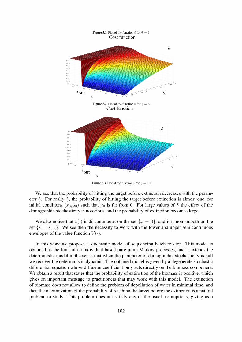
Figure 5.1. Plot of the function v for γ = 1

0

0.5

1

1.5

2

2.5

3

3.5

4

4.5

5 0

0.5

1

1.5

2

2.5

3

3.5

4

4.5

50

0.1

0.2

0.3

0.4

0.5

0.6

0.7

0.8

0.9

1

s

sout x

Cost function

v~

Figure 5.2. Plot of the function v for γ = 5

00.5

11.5

22.5

33.5

44.5

50

1

2

3

4

5

0

0.1

0.2

0.3

0.4

0.5

0.6

0.7

0.8

0.9

1

V

s

sout

x

Cost function

v~

Figure 5.3. Plot of the function v for γ = 10

We see that the probability of hitting the target before extinction decreases with the param-eter γ. For really γ, the probability of hitting the target before extinction is almost one, forinitial conditions (x0, s0) such that x0 is far from 0. For large values of γ the effect of thedemographic stochasticity is notorious, and the probability of extinction becomes large.

We also notice that v(·) is discontinuous on the set x = 0, and it is non-smooth on theset s = sout. We see then the necessity to work with the lower and upper semicontinuousenvelopes of the value function V (·).

In this work we propose a stochastic model of sequencing batch reactor. This model isobtained as the limit of an individual-based pure jump Markov processes, and it extends thedeterministic model in the sense that when the parameter of demographic stochasticity is nullwe recover the deterministic dynamic. The obtained model is given by a degenerate stochasticdifferential equation whose diffusion coefficient only acts directly on the biomass component.We obtain a result that states that the probability of extinction of the biomass is positive, whichgives an important message to practitioners that may work with this model. The extinctionof biomass does not allow to define the problem of depollution of water in minimal time, andthen the maximization of the probability of reaching the target before the extinction is a naturalproblem to study. This problem does not satisfy any of the usual assumptions, giving as a

102

result a discontinuous value function. We conjecture a Dynamic Programming Principle forthis problem. This is an ongoing work.

103

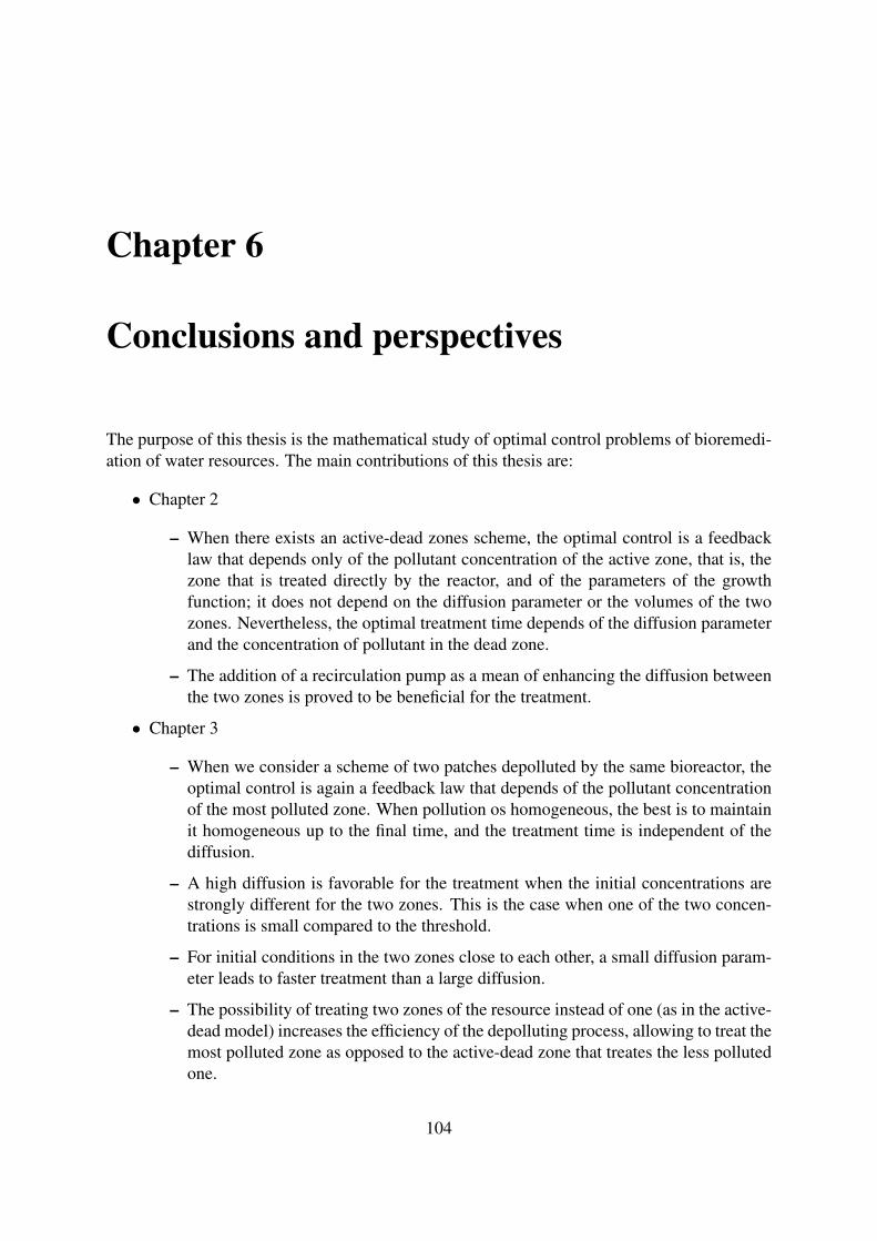
Chapter 6

Conclusions and perspectives

The purpose of this thesis is the mathematical study of optimal control problems of bioremedi-ation of water resources. The main contributions of this thesis are:

• Chapter 2

– When there exists an active-dead zones scheme, the optimal control is a feedbacklaw that depends only of the pollutant concentration of the active zone, that is, thezone that is treated directly by the reactor, and of the parameters of the growthfunction; it does not depend on the diffusion parameter or the volumes of the twozones. Nevertheless, the optimal treatment time depends of the diffusion parameterand the concentration of pollutant in the dead zone.

– The addition of a recirculation pump as a mean of enhancing the diffusion betweenthe two zones is proved to be beneficial for the treatment.

• Chapter 3

– When we consider a scheme of two patches depolluted by the same bioreactor, theoptimal control is again a feedback law that depends of the pollutant concentrationof the most polluted zone. When pollution os homogeneous, the best is to maintainit homogeneous up to the final time, and the treatment time is independent of thediffusion.

– A high diffusion is favorable for the treatment when the initial concentrations arestrongly different for the two zones. This is the case when one of the two concen-trations is small compared to the threshold.

– For initial conditions in the two zones close to each other, a small diffusion param-eter leads to faster treatment than a large diffusion.

– The possibility of treating two zones of the resource instead of one (as in the active-dead model) increases the efficiency of the depolluting process, allowing to treat themost polluted zone as opposed to the active-dead zone that treates the less pollutedone.

104

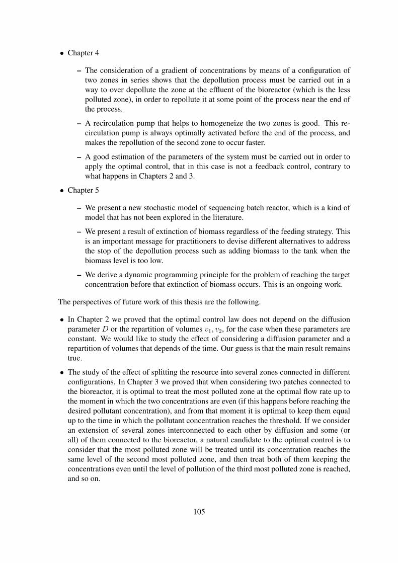
• Chapter 4

– The consideration of a gradient of concentrations by means of a configuration oftwo zones in series shows that the depollution process must be carried out in away to over depollute the zone at the effluent of the bioreactor (which is the lesspolluted zone), in order to repollute it at some point of the process near the end ofthe process.

– A recirculation pump that helps to homogeneize the two zones is good. This re-circulation pump is always optimally activated before the end of the process, andmakes the repollution of the second zone to occur faster.

– A good estimation of the parameters of the system must be carried out in order toapply the optimal control, that in this case is not a feedback control, contrary towhat happens in Chapters 2 and 3.

• Chapter 5

– We present a new stochastic model of sequencing batch reactor, which is a kind ofmodel that has not been explored in the literature.

– We present a result of extinction of biomass regardless of the feeding strategy. Thisis an important message for practitioners to devise different alternatives to addressthe stop of the depollution process such as adding biomass to the tank when thebiomass level is too low.

– We derive a dynamic programming principle for the problem of reaching the targetconcentration before that extinction of biomass occurs. This is an ongoing work.

The perspectives of future work of this thesis are the following.

• In Chapter 2 we proved that the optimal control law does not depend on the diffusionparameter D or the repartition of volumes v1, v2, for the case when these parameters areconstant. We would like to study the effect of considering a diffusion parameter and arepartition of volumes that depends of the time. Our guess is that the main result remainstrue.

• The study of the effect of splitting the resource into several zones connected in differentconfigurations. In Chapter 3 we proved that when considering two patches connected tothe bioreactor, it is optimal to treat the most polluted zone at the optimal flow rate up tothe moment in which the two concentrations are even (if this happens before reaching thedesired pollutant concentration), and from that moment it is optimal to keep them equalup to the time in which the pollutant concentration reaches the threshold. If we consideran extension of several zones interconnected to each other by diffusion and some (orall) of them connected to the bioreactor, a natural candidate to the optimal control is toconsider that the most polluted zone will be treated until its concentration reaches thesame level of the second most polluted zone, and then treat both of them keeping theconcentrations even until the level of pollution of the third most polluted zone is reached,and so on.

105

Consider a simple extension that consists of adding a third zone in the two patches modelstudied in Chapter 3. This third zone is adjacent to the other two zones that have accessto the bioreactor and is connected by diffusion with them, as Figure 6.1 shows.

q2

2v

rv

s , xrr bioreactor

biomass

settler

q

q2

q

D21s 2s

patch 2

D1

patch 1 patch 3

3s

q1

q1

q = q1+q

2

3v1v

Figure 6.1. First extension: model with three patches and two pumps

In this problem, we see that there is no direct way to depollute the intermediate zone,it must be depolluted in an indirect way through the control of the pollution in zones1 and 3. This is a problem whose velocity set is not convex, bringing the same issuesthat the problem studied in Chapter 3; it also has controllability issues, in the sense thatdepending on the parameters of the system, the configuration s1 = s2, s1 = s3, s2 = s3

cannot be maintained. It is also not clear what to do when the intermediate zone is themost polluted one. We would like to extend the results of Chapters 2-4 to several zonesconnected in different configurations, and to explore the effects of combining the paralleland series configurations to generate a more accurate model of inhomogeneity in theresource.

• In Chapter 3 we proved that despite of the velocity set being not convex, the solution ofthe relaxed problem is a non-convexified control. This is due to the particular structureof the dynamic that depends of two control parameters α and s?r , where α acts linearlyand s?r not.

– whenever s1 6= s2, the velocity set is not convex. Nevertheless, its extreme pointsare given by points parametrized by values α = 0 and s?r = s?r (s2), or α = 1 ands?r = s?r (s1), or s?r = 0 and α ∈ [0, 1]. This last option is not admissible.

– when s1 = s2, the velocity set becomes convex, so in this case there is no need ofconvexification.

An interesting possible future work can be to obtain results of Chapter 3 for systemswhose dynamics are governed by equations such that the velocity set is non-convex butsatisfy the previous property.

• Another natural extension of the work presented in this thesis concerns the study of thedepollution of a water resource polluted by two substrates. The water is treated by usinga continuous stirred bioreactor consisting of two zones. In the first zone the substrate of

106

type a is treated by a specific species of microorganism that degrades it and produces asa byproduct substrate of type b at a rate c ≥ 0. The substrate of type b is treated in thesecond zone by another microorganism species, and the treated effluent is returned to theresource, as in Figure 6.2. The problem consists of the treatment of the two substrates inthe resource in minimal time by controlling the flow rate Q.

Q

Q

Q

Q

Q

resource

bioreactor

Aerobic

zone

Anaerobic

zone

settler

biomass

Figure 6.2. Second extension: problem with two pollutants

In this problem it is also possible to suppose that the volume of the resource is largecompared to the volume of the reactor, which leads to a quasi-steady-state approximationof the dynamics. Here it is convenient to keepQ as a control variable instead of replacingit by the concentration of equilibrium in each zone of the bioreactor (as it was done inChapters 2-4). The equations that model the time evolution of this problem are given by

sa = Q (s?a1(Q, sa)− sa) ,sb = Q (s?b2(Q, sa, sb)− sb) ,

where s?a1(Q, sa) and s?b2(Q, sa, sb) are the corresponding concentrations of equilibriuminside each zone of the bioreactor, given by the formulas

s?a1(Q, sa) := min

µ−1

1

(Q

v1

), sa

,

s?b2(Q, sa, sb) := min

µ−1

2

(Q

v2

), c(sa − s?a1(Q, sa)) + sb

,

In this problem the velocity set is non-convex, and the Hamiltonian is non-smooth. Then,a relaxation of the problem must be performed, and tools such as the extended maximumprinciple of Pontryagin with subdifferentials must be used. We would like to study in afirst step the minimal time optimal control problem with constant volumes, and then, as asecond step, to extend the result to obtain the best initial repartition of volumes dependingof the initial state to perform the treatment in minimal time.

• In Chapter 5 we study and derive a dynamic programming principle for the problem ofthe maximization of the probability of attaining a target prior to extinction of biomass.

107

This is an ongoing work, and the next steps for this problem are to derive the Hamilton-Jacobi-Bellman (HJB) equation satified by the value function, to establish if the obtainedequation characterizes the value function, that is, if the value function is the unique vis-cosity solution of the HJB equation. This is a non-standard problem, because we workin an unbounded domain, with a differential operator that is degenerate and not elliptic,and the value function is discontinuous at the boundary of the domain. We expect tobe able to give some information about the optimal control and to solve numerically theHamilton-Jacobi-Bellman equation of the problem. Also, we expect to be able to provethe existence of solutions of the optimal control problem (Filippov’s like theorem).

• We intend to extend the study of the stochastic bioreactor model to the case of the chemo-stat. It will be interesting to compare a stochastic model of the chemostat obtained bymeans of the methods described in this thesis, taking into account demographic stochas-ticity, with those existing in the literature. We are also interested in the study of theoptimal control problem of maximizing the probability of reaching a target level of de-pollution prior to the extinction of the biomass, and to derive a dynamic programmingprinciple for this problem.

108

Bibliography

[1] E. Abulesz and G. Lyberatos. Periodic optimization of continuous microbial growth pro-cesses. Biotechnol. and Bioeng., 29:1059–1065, 1987.

[2] J. Alford. Bioprocess control: Advances and challenges. Computers and Chemical Engi-neering, 30:1464–1475, 2006.

[3] J. Banga, E. Balsa-Canto, C. Moles, and A. Alonso. Dynamic optimization of bioreactors:a review. Proceedings of the Indian Academy of Sciences, 69:257–265, 2003.

[4] S. Barbier, A. Rapaport, and A. Rousseau. Modelling of biological decontamination of awater resource in natural environment and related feedback strategies. Journal of Scien-tific Computing, pages 1–14, 2016.

[5] M. Bardi and I. Capuzzo-Dolcetta. Optimal control and viscosity solutions of Hamilton-Jacobi-Bellman equations. Systems & Control: Foundations & Applications. BirkhäuserBoston, Inc., Boston, MA, 1997. With appendices by Maurizio Falcone and PierpaoloSoravia.

[6] G. Bastin, D. Nesic, Y. Tan, and I. Mareels. On extremum seeking in bioprocesses withmultivalued cost functions. Biotechnology Progress, 25(3):683–689, 2009.

[7] J.V. Baxley and S.B. Robinson. Differential equations and computational simulations iicoexistence in the unstirred chemostat. Applied Mathematics and Computation, 89(1):41– 65, 1998.

[8] R. Boopathy. Factors limiting bioremediation technologies. Bioresource Technology,74(1):63 – 67, 2000.

[9] V. F. Borisov and M. I. Zelikin. Theory of chattering control. Systems & Control: Foun-dations & Applications. Birkhäuser Boston, Inc., Boston, MA, 1994. With applicationsto astronautics, robotics, economics, and engineering.

[10] B. Bouchard and M. Nutz. Weak dynamic programming for generalized state constraints.SIAM J. Control Optim., 50(6):3344–3373, 2012.

[11] B. Bouchard and N. Touzi. Weak dynamic programming principle for viscosity solutions.SIAM J. Control Optim., 49(3):948–962, 2011.

109

[12] G. J. Butler and G. S. K. Wolkowicz. A mathematical model of the chemostat with a gen-eral class of functions describing nutrient uptake. SIAM Journal on Applied Mathematics,45(1):138–151, 1985.

[13] G.J. Butler, S.B. Hsu, and P. Waltman. A mathematical model of the chemostat withperiodic washout rate. SIAM Journal on Applied Mathematics, 45(3):435–449, 1985.

[14] F. Campillo and C. Fritsch. Weak convergence of a mass-structured individual-basedmodel. Applied Mathematics & Optimization, 72(1):37–73, 2015.

[15] F. Campillo, M. Joannides, and I. Larramendy-Valverde. Stochastic modeling of thechemostat. Ecological Modelling, 222(15):2676 – 2689, 2011.

[16] T. Caraballo, X. Han, and P.E. Kloeden. Chemostats with random inputs and wall growth.Math. Methods Appl. Sci., 38(16):3538–3550, 2015.

[17] L. Cesari. Optimization—theory and applications, volume 17 of Applications of Mathe-matics (New York). Springer-Verlag, New York, 1983. Problems with ordinary differentialequations.

[18] J. Claisse, D. Talay, and X. Tan. A Pseudo-Markov Property for Controlled DiffusionProcesses. SIAM J. Control Optim., 54(2):1017–1029, 2016.

[19] F. H. Clarke. Optimization and nonsmooth analysis, volume 5 of Classics in AppliedMathematics. Society for Industrial and Applied Mathematics (SIAM), Philadelphia, PA,second edition, 1990.

[20] P. Collet, S. Martínez, S. Méléard, and J. San Martín. Stochastic models for a chemostatand long-time behavior. Adv. in Appl. Probab., 45(3):822–837, 09 2013.

[21] R. Crab, Y. Avnimelech, T. Defoirdt, P. Bossier, and W. Verstraete. Nitrogen removaltechniques in aquaculture for a sustainable production. Aquaculture, 270(1-4):1 – 14,2007.

[22] G. D’Ans, D. Gottlieb, and P. Kokotovic. Optimal control of bacterial growth. Automat-ica, 8:729–736, 1972.

[23] G. D’Ans, P. Kokotovic, and D. Gottlieb. Time-optimal control for a model of bacterialgrowth. J. Optim. Theory Appl., 7(1):61–69, 1971.

[24] S. Diehl and S Farås. Control of an ideal activated sludge process in wastewater treatmentvia an ode-pde model. Journal of Process Control, 23(3):359 – 381, 2013.

[25] S. Diehl and S. Farås. A reduced-order ODE-PDE model for the activated sludge pro-cess in wastewater treatment: classification and stability of steady states. Math. ModelsMethods Appl. Sci., 23(3):369–405, 2013.

[26] D. Dochain. Automatic control of bioprocesses. John Wiley & Sons, 2013.

110

[27] D. Dochain and P. Vanrolleghem. Dynamical modelling and estimation in wastewatertreatment processes. IWA publishing, 2001.

[28] E.H. Eding, A. Kamstra, J.A.J. Verreth, E.A. Huisman, and A. Klapwijk. Design andoperation of nitrifying trickling filters in recirculating aquaculture: A review. Aquacul-tural Engineering, 34(3):234 – 260, 2006. Design and Selection of Biological Filters forFreshwater and Marine Applications.

[29] V. Estrada, E.R. Parodi, and M. S. Diaz. Addressing the control problem of algae growthin water reservoirs with advanced dynamic optimization approaches. Computers andChemical Engineering, 33:2063–2074, 2009.

[30] S. N. Ethier and T. G. Kurtz. Markov processes. Wiley Series in Probability and Mathe-matical Statistics: Probability and Mathematical Statistics. John Wiley & Sons Inc., NewYork, 1986. Characterization and convergence.

[31] P. Gajardo, J. Harmand, H. Ramírez C., and A. Rapaport. Minimal time bioremediationof natural water resources. Automatica J. IFAC, 47(8):1764–1769, 2011.

[32] P. Gajardo, H. Ramírez, and A. Rapaport. Minimal time sequential batch reactors withbounded and impulse controls for one or more species. SIAM Journal on Control andOptimization, 47(6):2827–2856, 2008.

[33] P. Gajardo, H. Ramírez, V. Riquelme, and A. Rapaport. Bioremediation of natural waterresources via optimal control techniques. In BIOMAT 2011, pages 178–190. World Sci.Publ., Hackensack, NJ, 2012.

[34] R.D. Gulati and E. van Donk. Lakes in the Netherlands, their origin, eutrophication andrestoration: state of the art review. Hydrobiologia, 478:73–106, 2002.

[35] K. Hamza and F. C. Klebaner. Conditions for integrability of Markov chains. J. Appl.Probab., 32(2):541–547, 1995.

[36] G. Hardin. The competitive exclusion principle. Science, 131(3409):1292–1297, 1960.

[37] D. Herbert, R. Elsworth, and R. C. Telling. The continuous culture of bacteria; a theoret-ical and experimental study. Journal of General Microbiology, 14(3):601–622, 1956.

[38] J. Hong. Optimal substrate feeding policy for fed batch fermentation with substrate andproduct inhibition kinetics. Biotechnol. Bioengng., 28:1421–1431, 1986.

[39] S. B. Hsu, H. L. Smith, and P. Waltman. Dynamics of competition in the unstirred chemo-stat. Canad. Appl. Math. Quart, 2:461–483, 1994.

[40] N. Ikeda and S. Watanabe. Stochastic differential equations and diffusion processes, vol-ume 24 of North-Holland Mathematical Library. North-Holland Publishing Co., Amster-dam, 1981.

[41] L. Imhof and S. Walcher. Exclusion and persistence in deterministic and stochastic

111

chemostat models. J. Differential Equations, 217(1):26–53, 2005.

[42] I. Van Impe and G. Bastin. Optimal adaptive control of fedbatch fermentation processes.Control Eng. Practice, 3:939–954, 1995.

[43] J. Van Impe and G. Bastin. Optimal adaptive control of biotechnological processes, pages401–436. Kluwer Academic Publishers, 1998.

[44] R.L. Irvine and A.W. Busch. Sequencing batch biological reactors: An overview. Journalof Water Pollution Control Federation, 51(2):235–243, 1979.

[45] R.L. Irvine and L.H. Ketchum. Sequencing batch reactors for biological waste-watertreatment. CRC Critical Reviews in Envirnomental Control, 18(4):255–294, 1988.

[46] A. Joffe and M. Métivier. Weak convergence of sequences of semimartingales with appli-cations to multitype branching processes. Adv. in Appl. Probab., 18(1):20–65, 1986.

[47] A. Johnson. The control of fed-batch fermentation processes: a survey. Automatica,23(6):691–705, 1987.

[48] I. Karatzas and S. E. Shreve. Brownian motion and stochastic calculus, volume 113 ofGraduate Texts in Mathematics. Springer-Verlag, New York, second edition, 1991.

[49] H.K. Khalil. Nonlinear Systems. Pearson Education. Prentice Hall, 2002.

[50] P. Kittisupakorn and M. Hussain. Comparison of optimisation based control techniquesfor the control of a cstr. International Journal of Computer Applications in Technology,13(3–5):178–184, 2000.

[51] Z. Kurtanjek. Optimal nonsingular control of fed-batch fermentation. Biotechnology andBioengineering, 37:814–823, 1991.

[52] D. Lamberton and B. Lapeyre. Introduction to stochastic calculus applied to finance.Chapman & Hall, London, 1996. Translated from the 1991 French original by NicolasRabeau and François Mantion.

[53] H.C. Lim, Y.J. Tayeb, J.M. Modak, and P. Bonte. Computational algorithms for optimalfeed rates for a class of fed-batch fermentation: numerical results for penicillin and cellproduction. Biotechnology and Bioengineering, 28(9):1408–1420, 1986.

[54] N. Marcos, M. Guay, D. Dochain, and T. Zhang. Adaptive extremum seeking control ofa continuous stirred tank bioreactor with Haldane’s kinetics. Journal of Process Control,14:317–328, 2004.

[55] D. Mazouni, J. Harmand, A. Rapaport, and H. Hammouri. Optimal time switching controlfor multi-reaction batch process. Optimal Control Applications and Methods, 31:289–301, 2010.

[56] S. Méléard and D. Villemonais. Quasi-stationary distributions and population processes.

112

Probab. Surveys, 9:340–410, 2012.

[57] P. Mohajerin Esfahani, D. Chatterjee, and J. Lygeros. The stochastic reach-avoid problemand set characterization for diffusions. Automatica J. IFAC, 70:43–56, 2016.

[58] J. Monod. Recherches sur la croissance des cultures bacteriennes. Paris: Herman, 1942.

[59] J. Monod. La technique de la culture continue, théorie et applications. Annales del’Institut Pasteur, 79(4):390–410, 1950.

[60] J. Moreno. Optimal time control of bioreactors for the wastewater treatment. OptimalControl Appl. Methods, 20(3):145–164, 1999.

[61] M. Moreno C., A. González B., and MJ. Blanco S. Biological treatments for contaminatedsoils: hydrocarbon contamination. fungal applications in bioremediation treatment. RevIberoam Micol, 21(3):103–20, 2004. Review. Spanish.

[62] MA New England Interstate Water Pollution Control Commission, Lowell. Sequencingbatch reactor design and operational considerations. 2005.

[63] A. Novick and L. Szilard. Experiments with the chemostat on spontaneous mutations ofbacteria. Proc Natl Acad Sci U S A., 36(12):708–719, December 1950.

[64] R. H. Piedrahita. Reducing the potential environmental impact of tank aquaculture ef-fluents through intensification and recirculation. Aquaculture, 226(1-4):35 – 44, 2003.Management of Aquaculture Effluents.

[65] R.S. Ramalho. Introduction to Wastewater Treatment Processes. Academic Press, SanDiego, second edition, 1983.

[66] H. Ramírez, A. Rapaport, and V. Riquelme. Optimal Feedback Synthesis and MinimalTime Function for the Bioremediation of Water Resources with Two Patches. SIAM J.Control Optim., 54(3):1697–1718, 2016.

[67] K. Rani and V. Rao. Control of fermenters: a review. Bioprocess Engineering, 21:77–88,1999.

[68] R.T. Rockafellar and Roger J.B. Wets. Variational analysis, volume 317 of Grundlehrender Mathematischen Wissenschaften [Fundamental Principles of Mathematical Sci-ences]. Springer-Verlag, Berlin, 1998.

[69] L. Ruan and X. Chen. Comparison of several periodic oscillations of a continuous fer-mentation process. Biotechnol. Progr., 12:1059–1065, 1996.

[70] S. Shioya. Optimization and control in fed-batch bioreactors, pages 111–142. Advancesin Biochemical Engineering & Biotechnology, Ed. J. Van Impe, P. Vanrolleghem and D.Iserentant. Springer Berlin, Heidelberg, 1992.

[71] I. Smets, J. Claes, E. November, G. Bastin, and I. Van Impe. Optimal adaptive control of

113

(bio)chemical reactors: past, present and future. Journal of Process Control, 14:795–805,2004.

[72] I. Smets and I. Van Impe. Optimal control of (bio-)chemical reactors: generic propertiesof time and space dependent optimization. Mathematics and Computers in Simulation,60(6):475–486, 2002.

[73] H. L. Smith and P. Waltman. The theory of the chemostat, volume 13 of Cambridge Stud-ies in Mathematical Biology. Cambridge University Press, Cambridge, 1995. Dynamicsof microbial competition.

[74] H.L. Smith. Monotone dynamical systems, volume 41 of Mathematical Surveys andMonographs. American Mathematical Society, Providence, RI, 1995. An introductionto the theory of competitive and cooperative systems.

[75] M. Sondergaard, E. Jeppesen, T.L. Lauridsen, C. Skov, E.H. van Nes, R. Roijackers,E. Lammens, and R. Portielje. Lake restoration: successes, failures and long term effects.Journal of Applied Ecology, 44:1095–1105, 2007.

[76] A. Soukkou, A. Khellaf, S. Leulmi, and K. Boudeghdegh. Optimal control of a CSTRprocess. Brazilian Journal of Chemical Engineering, 25:799 – 812, 12 2008.

[77] D. Spitzer. Maximization of steady-state bacterial production in a chemostat with ph andsubstrate control. Biotechnology and Bioengineering, 18(2):167–178, 2004.

[78] B. Srinivasan, S. Palanki, and D. Bonvin. Dynamic optimization of batch processes: I.characterization of the nominal solution. Computers & Chemical Engineering, 27(1):1 –26, 2003.

[79] G. Stephanopoulos, A. G. Frederickson, and R. Aris. The growth of competing microbialpopulations in a cstr with periodically varying inputs. AIChE Journal, 25(5):863–872,1979.

[80] N. Touzi. Optimal stochastic control, stochastic target problems, and backward SDE, vol-ume 29 of Fields Institute Monographs. Springer, New York; Fields Institute for Researchin Mathematical Sciences, Toronto, ON, 2013. With Chapter 13 by Angès Tourin.

[81] R.G. Tsoneva, T.D. Patarinska, and I.P. Popchev. Augmented lagrange decompositionmethod for optimal control calculation of batch fermentation processes. Bioprocess andBiosystems Engineering, 18(2):143–153, 1998.

[82] V. Van Breusegem and G. Bastin. Reduced order dynamical modelling of reaction sys-tems: a singular perturbation approach. In Decision and Control, 1991., Proceedings ofthe 30th IEEE Conference on, pages 1049–1054. IEEE, 1991.

[83] R. Vinter. Optimal control. Systems & Control: Foundations & Applications. BirkhäuserBoston, 2000.

114

[84] H. Wang, M. Krstic, and G. Bastin. Optimizing bioreactors by extremum seeking. Inter-national Journal of Adaptive Control and Signal Processing, 13:651–669, 1999.

[85] J. Yong and X. Y. Zhou. Stochastic controls, volume 43 of Applications of Mathematics(New York). Springer-Verlag, New York, 1999. Hamiltonian systems and HJB equations.

[86] T. Zhang, M. Guay, and D. Dochain. Adaptive extremum seeking control of continuousstirred-tank bioreactors. AIChE Journal, 49(1):113–123, 2003.

115