Delft University of Technology

Delft Center for Systems and Control

Technical report 11-044

Optimal coordination of a multiple HVDC

link system using centralized and

distributed control∗

P. Mc Namara, R.R. Negenborn, B. De Schutter, and G. Lightbody

If you want to cite this report, please use the following reference instead:

P. Mc Namara, R.R. Negenborn, B. De Schutter, and G. Lightbody, “Optimal coor-

dination of a multiple HVDC link system using centralized and distributed control,”

IEEE Transactions on Control Systems Technology, vol. 21, no. 2, pp. 302–314, Mar.

2013.

Delft Center for Systems and Control

Delft University of Technology

Mekelweg 2, 2628 CD Delft

The Netherlands

phone: +31-15-278.51.19 (secretary)

fax: +31-15-278.66.79

URL: http://www.dcsc.tudelft.nl

∗This report can also be downloaded via http://pub.deschutter.info/abs/11_044.html

1

Optimal coordination of a multiple HVDC link

system using centralised and distributed controlPaul Mc Namara, Student Member, IEEE, Rudy R. Negenborn, Bart De Schutter, Senior Member, IEEE,

Gordon Lightbody

Abstract—This paper presents both off-line and on-line optimi-sation techniques for the control of a multiple High Voltage DirectCurrent link power system. A frequency control scheme basedon classical PID controllers is proposed and optimally tunedoff-line using Particle Swarm Optimisation. The performance ofthis scheme is compared with the performance of a centralisedModel Predictive Control (MPC) scheme, and a distributed MPCscheme that uses only local communications. The results illustratethat a significant performance improvement can be achievedusing distributed MPC instead of classical control, illustrating thepotential of distributed MPC for use in future power networks.

Index Terms—Distributed control, Model Predictive Control,HVDC, multi-agent systems, Particle Swarm Optimisation.

I. INTRODUCTION

POWER networks are large, complex, highly intercon-

nected systems. As increasing demands are imposed on

power networks, more advanced control techniques are needed

in order to maintain network stability. This can be achieved by

installing power system devices such as Flexible Alternating

Current Transmission Systems (FACTSs) and High Voltage

Direct Current (HVDC) links [1] while using more advanced

control systems to maximise network efficiency. HVDC links

allow for the efficient transmission of large quantities of power

over long distances and can be used to improve transient

stability and power system damping [1].

In [2], a multiple HVDC link system based on part of the

Nordic power grid was presented. This is a nonlinear, MIMO

dynamic system. The power generated in the system is kept

constant and the modulation of the HVDC links alone is then

used to restabilise the system after line faults. Thus there

is a high level of interconnectivity between subsystems in

this model. So far, centralised control techniques that were

not based on optimisation, were used to control this system.

These techniques focused on damping out oscillations between

the AC connected areas, and were based on proportional

control [2] and feedback linearisation [3]. However, while

these controllers stabilised the system, there was significant

scope for improving performance. Also, centralised control

Paul Mc Namara (paulmcn@rennes.ucc.ie) and Gordon Lightbody(g.lightbody@ucc.ie) are with the Control and Intelligent Systems Groupin the Electrical and Electronic Engineering Department, University CollegeCork, Ireland.

Rudy R. Negenborn (r.r.negenborn@tudelft.nl) is with the Departmentof Marine and Transport Technology, Delft University of Technology, TheNetherlands.

Bart De Schutter (b.deschutter@tudelft.nl) is with the Delft Center forSystems and Control, Delft University of Technology, The Netherlands.

approaches for such systems may not always be possible, in

the case of a deregulated power market for example.

Off-line optimisation techniques are often used to optimise

parameters of a control system in order to maximise system

performance based on certain criteria. Stochastic search tech-

niques such as Simulated Annealing [4], Genetic Algorithms

[5], and Particle Swarm Optimisation (PSO) [6] have proven

to be efficient ways of finding globally optimal solutions for

controller gains. Due to their ability to find global optima,

Genetic Algorithms have proven to be particularly popular as

a tool for finding optimal gains [7, 8, 5]. However, recently

the advantages of using PSO over Genetic Algorithms for the

optimisation of PID gains have been demonstrated, in terms

of both the quality of and the efficiency with which a final

solution can be found [6].

On-line optimisation techniques, such as Model Predictive

Control (MPC) [9], use real-time optimisation in order to

determine the control inputs for systems. One of the main

advantages of MPC, over non-optimisation based techniques,

is the systematic and intuitive manner in which constraints are

incorporated into the control system and the fact that delays

are naturally catered for. It is a mature technology at this stage,

with stability and robustness analysis well established [10,11,

12].

However, for large systems such as the electricity grid, it is

often impractical to implement MPC from a central controller,

due to computational constraints. Likewise it is often desirable

or necessary to use a number of separate controllers, called

agents, to control subsystems, e.g., in a deregulated power

market several controllers may be responsible for the control

of different sections of the power grid, or when power systems

span several countries, countries will typically have separate

controllers for their own sections of the grid.

There has been much research interest in recent years

in distributed MPC [13, 14, 15], in which several agents

communicate and cooperate with each other to approximate

the behaviour of a centralised MPC agent. Lyapunov-based

MPC techniques [15,16], game-theoretic approaches [14], and

iterative techniques based on the decomposition of the original

control problem into several smaller problems [17,18] have all

been used to distribute the control amongst agents.

The performance of a centralised MPC scheme, which

reaches a Pareto equilibrium, can be achieved in a distributed

way if all agents in a system have all the information of a

centralised MPC made available to them (assuming convex

cost functions), i.e., the goals of all agents in a system,

knowledge of the full state-space of the system, all system

2

constraints, etc. [18, 14]. However, in vast complex systems,

such as electricity grids, the communication of this volume of

information is impractical or may not even be possible, e.g., in

a deregulated power market control agents may not be willing

to share this level of information with other control agents.

However, when communication of interconnecting variables

is allowed between adjacent agents, a Nash equilibrium can

be achieved [14]. While Nash equilibrium seeking control

systems, in general, do not achieve the performance of a

Pareto equilibrium seeking control system, typically their

performance will be significantly better than that achieved

by a decentralised control system with no communications

[18]. Indeed, promising results have already been achieved

controlling power networks, which include FACTS devices,

with control agents that only communicate with agents to

which they are connected by a common variable [19, 18, 20].

In this paper, three optimisation-based control techniques

are proposed for the control of the Nordic multiple HVDC link

system. The controllers used are an off-line PSO-optimised

PID controller, a centralised MPC controller, and a distributed

MPC controller that uses only local communications [17].

Typically distributed MPC systems will try to reach consen-

sus on interconnecting variables between agents. However in

the example in this paper all 4 agents share the same 2 control

inputs. Thus, we elaborate on how the control system in [17]

is used in order to coordinate the agents’ responses for control

inputs that are common to multiple agents.

As distributed MPC provides a scalable MPC architecture

that could realistically be used in large-scale power systems,

it is interesting to see how its performance compares with that

of an optimised centralised classical PID controller, given the

widespread use of PID controllers within the power industry.

As part of this analysis, however, it is necessary to take

into account the computational and communication overhead

associated with distributed MPC to get a better idea of the

trade-offs involved when using distributed MPC.

This paper is organised as follows. The multiple HVDC

link system is presented in Section II. The off-line PSO

optimisation of the PID gains of the multiple HVDC link

controller is presented in Section III. MPC and distributed

MPC are introduced in Section IV. Simulation studies compare

the performance of the different approaches in Section V.

Section VI contains conclusions and directions for future

research.

II. THE MULTIPLE HVDC LINK SYSTEM

The continuous-time dynamics of the multiple HVDC link

system under study here are described in this section.

A. Multiple HVDC link system description

The system, which is based on the multiple HVDC link

system between Denmark, Norway, and Sweden, is depicted in

Fig. 1 [21]. It consists of 4 buses with their own generation and

loads. Both Alternating Current (AC) and HVDC links connect

the buses. The HVDC links are of the Line Commutated

Converter type [22]. Generation capacities and loads are kept

constant in this paper. Large amounts of power are transferred

SS SS

Generator 1

Generator 2 Generator 3

Generator 4

Bus 1 Bus 4

Bus 3Bus 2

Load 2

Load 1 Load 4

Load 3

AC Line 1

AC Line 2

AC Line 3AC Line 4

HVDC Line 1 HVDC Line 2

SS SS SS SS

SS SS

Agent 1: Denmark 1

Agent 2: Norway Agent 3: Sweden

Agent 4: Denmark 2

Fig. 1. The multiple HVDC link system with areas controlled by agents[21].

from bus 2, which has the largest generation capacity, to bus

4, which has the largest power load.

B. Modelling

The classical swing equations for a generator a are [1]:

d

dtδra(t) = ω0∆ωra(t) (1)

d

dtωra(t) =

1

2Ha

(Pma(t)− PGa(t)−Da∆ωra(t)), (2)

where δra(t) is the rotor angle (rad), Ha is the inertial constant

(s), ωra(t) is the rotor speed (per unit), ∆ωra(t)= ωra(t)−1 is

the rotor speed deviation (per unit), ω0 is the base rotor speed

(rad/s), Pma(t) and PGa(t) are the mechanical and generated

power (per unit), respectively, and Da is the damping factor

(per unit).

The current injected by generator a,−→Iga(t), is given by:

−→Iga(t) =

−→E

′

qa(t)−−→Ua(t)

jx′

da

, (3)

where−→E

′

qa(t) = E′

qa(t)∠δa(t) is the internal voltage (per

unit) with magnitude E′

qa(t) and angle δa(t),−→Ua(t) =

Ua(t)∠θa(t) is the voltage (per unit) at the bus to which the

generator is connected with magnitude Ua(t) and angle θa(t),and x

′

dais the d-axis transient reactance. All variables are

defined as in the standard reference work [1]. The generated

power is then given by:

PGa(t) = R[−→Ega(t)

−→I ∗ga(t)]. (4)

Equations (1) and (2) of the classical model of a syn-

chronous generator assume that E′

qa(t) is constant [1]. These

classical equations are suitable for analysis of power oscilla-

tions and transient stability studies.

A π-model representation [1] of the AC links is used, as

in Fig. 2, where XLiis the line reactance, XSi is the shunt

reactance, XGiis a ground reactance (used here to simulate

3-phase to ground faults in the middle of line i), XBiis a

3

reactance (used here to simulate a line break), UL1and UL2

are the voltages on either side of line i, and Umiis the voltage

at the middle of the line connected to ground through XGi.

The value of XGidecreases from ∞ in the non-fault state

to 0 in the case of the 3-phase fault. As the faults happen in

the middle of the line, the line reactance is divided in half

on either side of the ground fault “line”. The value of XBi

increases from a value of 0 to ∞ when a line break is applied.

UL1U L2

Umi

XLi

2

XLi

2

XGiXSi

XSi

XBi

Fig. 2. π-model of lines.

A number of simplifications are made to the power system

model, subsequently reducing the complexity of the MPC

problem proposed in the next section, and making it faster,

without neglecting the system dynamics most relevant to

system stability.

• Loads are modelled as constant impedances.

• HVDC power transmission is considered instantaneous.

• The HVDC reactive power is taken as proportional to

HVDC active power.

The details of these simplifications are given in the following

paragraphs.

Loads are modelled as constant impedances in the

impedance matrix, i.e. with−→Sa = PLL

a +jQLLa , the consumed

complex load power in VA, the load impedance−→XLL

a is given

by

−→XLL

a =

−→Ua

−→U ∗a

−→S ∗a

. (5)

The HVDC link model in [21] is used to simplify the rep-

resentation of the system dynamics. This idealised version of

the HVDC link assumes instantaneous, lossless power delivery

and power factors that are equal on both the inverter and

rectifier sides. Thus, when active power injections from a

HVDC link j are applied to a bus in this model, the bus

receives +PDCj , where PDC

j is the active power in the HVDC

link. Equally, the bus from which the HVDC active power is

being sent then loses PDCj . This model is further simplified by

assuming that a simple controller structure is used as in [22],

such that QDCj = qrjP

DCj , where qrj is a constant, and QDC

j

is the reactive HVDC power in HVDC link j. An additional

simplification adopted in this paper is to directly calculate and

apply the HVDC powers. However, in a real system, currents

are injected that are calculated from these powers [1].

The internal node representation is used to model the system

dynamics [21] as it allows the power system to be represented

using a system of first-order differential equations. This is done

by rearranging the impedance matrix of the power network

so as to find its generator currents in terms of the network

voltages and HVDC currents, and then substituting the values

for these currents into the generator swing equations. This

is demonstrated in the following paragraphs. To do this it is

assumed that Pma is constant and that the loads are modelled

as constant impedances.

An impedance matrix gives the relationship between the

voltage nodes and currents in a power system. Lines and

loads are then represented by impedances in this matrix.

Consider the ath bus, with n voltage nodes and m HVDC

links connected to it. Then using Kirchhoff’s current law:

n∑

l=1

~Ya,l~Ul − ~Iga −

m∑

j=1

~IDCa, j= 0, (6)

where ~Ya,l =1

~Xa,l

, where ~Xa,l is the impedance between bus

a and voltage node l and ~IDCa, jis the current injected into

bus a from HVDC link j. This is repeated for all voltage nodes

in the network.

Using (6), an impedance matrix is constructed, based on

models for the AC lines, the generators, and the loads, as

described in the previous paragraphs:

Ig

IDC

0

=

Y A Y B 0

Y C Y D Y E

0 Y F Y G

E

U

Um

, (7)

where Ig = [~Ig1 , . . . ,~Ign ]

T, E = [ ~E′

q1, . . . , ~E

′

qn ]T,

U = [~U1, . . . , ~Un]T and Um = [~Um1

, . . . , ~Umb]T where

b is the number of AC lines in the system and IDC =[~IDC1, 1

, . . . , ~IDCn,m ]T.

From (7) the following can be found for Ig in terms of IDC

and E:

Ig = (Y A − Y B(Y D − Y EY−1G Y F))E

+ Y B(Y D − Y EY−1G Y F)

−1IDC

= (G+ jB)E + Y DCIDC

(8)

where G=R[Y A − Y B(Y D − Y EY−1G Y F)], B=I[Y A −

Y B(Y D − Y EY−1G Y F)], and YDC=Y D − Y EY

−1G Y F.

The following swing equation for generator a can be derived

using (2), (4), and (8):

d

dtωra =

1

2Ha

(

Pma −Ga,aE′2qa−

n∑

l=1l 6=a

E′

qaE′

ql(Ga,l cos(δra − δrl) +Ba,l sin(δra − δrl))

+ ga,1PDC1 + . . .+ ga,mPDC

m −Da∆ωra

)

,

(9)

where ga,j is the coefficient of the contribution of the power

injections from HVDC link j at bus a.

C. Definition of an agent

For clarity the definition of an agent, as understood in this

paper, will now be provided. An agent is defined here as an

entity responsible for the control of a system or subsystem,

with access to the current state of the system or subsystem it

controls. Agents have access to a model of the local system

4

or subsystem and in the distributed case, agents are able to

communicate with other agents who share a common variable.

Agents compute values for their control inputs at discrete time

steps based on the information available to them.

D. Control goals for the multiple HVDC link system

It is desirable to install a control system that maintains the

rotor frequencies as close as possible to 1 pu at all times for the

multiple link HVDC system. In this work the base frequency

is 50 Hz, the minimum allowable frequency is 49.2 Hz, and

the maximum allowable frequency is 50.8 Hz [23]. In per unit

terms it is therefore desired to keep the frequency between

0.984 pu and 1.016 pu. The total generated power equals the

total consumed power in the network, and so the modulation of

the HVDC link powers alone should be sufficient to restabilise

the generator frequencies at each bus, and return them to their

desired setpoints after frequency deviations are incurred due

to line fault disturbances.

Also the need for a multi-agent approach for controlling

this system could arise. Consider that 2 different agents are re-

sponsible for the areas in Denmark due to market deregulation;

usually controllers do not cross borders and so another 2 agents

could be responsible for the control of the areas in Norway and

Sweden, leading to a situation where 4 agents are responsible

for the control of this power network. Also, these agents all

share the same inputs, and the AC-line connected agents are

affected by their connected agent’s generator rotor positions,

and so the control problems of all agents in the system

are highly interconnected. For this reason several different

centralised and non-centralised control schemes are applied

to the system in this paper.

III. OFF-LINE PSO OPTIMISATION OF A CENTRALISED

PID CONTROL SCHEME

Proportional controllers were initially proposed in [21] for

control of the multiple HVDC link system, using the control

scheme presented in Fig. 3. The proportional gains and filter

bandwidths were chosen based on trial and error, observing

which combinations of values gave a good damping response.

However there is the potential for improved control perfor-

mance by using Proportional, Integral and Derivative (PID)

controllers, and then optimising both the controller gains and

the filter bandwidths, based on simulation runs of the power

network, using a suitable tuning criterion.

As simulations of the power network, which is represented

by a non-linear model, are used to provide the input to the

tuning criterion, the derivation of the relationship between

the PID gains and the tuning criterion is non-trivial and so

a derivative-free optimisation technique is used. Due to the

non-convex nature of these tuning problems, it is desirable

to use an optimisation technique that does not get trapped in

local minima.

Stochastic search techniques such as Simulated Annealing

[4], Genetic Algorithms [5], and Particle Swarm Optimisation

[6] have previously been quite successful in finding optimal

controller gains. PSO has been shown to outperform other

stochastic search algorithms, such as Genetic Algorithms, in

terms of both the quality of the solutions found and the time

needed to find them [6]. Hence, PSO is used in this work.

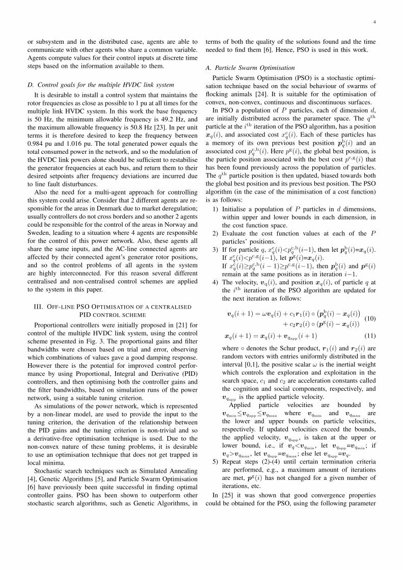
A. Particle Swarm Optimisation

Particle Swarm Optimisation (PSO) is a stochastic optimi-

sation technique based on the social behaviour of swarms of

flocking animals [24]. It is suitable for the optimisation of

convex, non-convex, continuous and discontinuous surfaces.

In PSO a population of P particles, each of dimension d,

are initially distributed across the parameter space. The qth

particle at the ith iteration of the PSO algorithm, has a position

xq(i), and associated cost xcq(i). Each of these particles has

a memory of its own previous best position pbq (i) and an

associated cost pc,bq (i). Here pg(i), the global best position, is

the particle position associated with the best cost pc,g(i) that

has been found previously across the population of particles.

The qth particle position is then updated, biased towards both

the global best position and its previous best position. The PSO

algorithm (in the case of the minimisation of a cost function)

is as follows:

1) Initialise a population of P particles in d dimensions,

within upper and lower bounds in each dimension, in

the cost function space.

2) Evaluate the cost function values at each of the Pparticles’ positions.

3) If for particle q, xcq(i)<pc,bq (i−1), then let pb

q (i)=xq(i).If xc

q(i)<pc,g(i−1), let pg(i)=xq(i).If xc

q(i)≥pc,bq (i − 1)≥pc,g(i−1), then pbq (i) and pg(i)

remain at the same positions as in iteration i−1.

4) The velocity, vq(i), and position xq(i), of particle q at

the ith iteration of the PSO algorithm are updated for

the next iteration as follows:

vq(i+ 1) = ωvq(i) + c1r1(i) (

pbq (i)− xq(i)

)

+ c2r2(i) (pg(i)− xq(i))

(10)

xq(i+ 1) = xq(i) + vqapp(i+ 1) (11)

where denotes the Schur product, r1(i) and r2(i) are

random vectors with entries uniformly distributed in the

interval [0,1], the positive scalar ω is the inertial weight

which controls the exploration and exploitation in the

search space, c1 and c2 are acceleration constants called

the cognition and social components, respectively, and

vqapp is the applied particle velocity.

Applied particle velocities are bounded by

vqmin≤vqapp≤vqmax

where vqminand vqmax

are

the lower and upper bounds on particle velocities,

respectively. If updated velocities exceed the bounds,

the applied velocity, vqapp , is taken at the upper or

lower bound, i.e., if vq<vqmin, let vqapp=vqmin

; if

vq>vqmax, let vqapp=vqmax

; else let vqapp=vq .

5) Repeat steps (2)-(4) until certain termination criteria

are performed, e.g., a maximum amount of iterations

are met, pg(i) has not changed for a given number of

iterations, etc.

In [25] it was shown that good convergence properties

could be obtained for the PSO, using the following parameter

5

∆PDC2

PDC1,0

PDC2,0

+

+

+

+

∆PDC1

+

+

+

+

PID1

PID2

s/ω214

s2+Bs+ω214

s/ω232

s2+Bs+ω232

Bandpass filter ω14

Bandpass filter ω32

ω0

ω0

+

-

+

-ω2

ω1

ω3

ω4

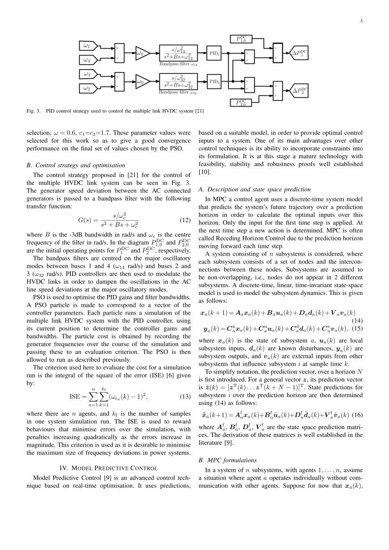
Fig. 3. PID control strategy used to control the multiple link HVDC system [21]

selection; ω = 0.6, c1=c2=1.7. These parameter values were

selected for this work so as to give a good convergence

performance on the final set of values chosen by the PSO.

B. Control strategy and optimisation

The control strategy proposed in [21] for the control of

the multiple HVDC link system can be seen in Fig. 3.

The generator speed deviation between the AC connected

generators is passed to a bandpass filter with the following

transfer function:

G(s) =s/ω2

c

s2 +Bs+ ω2c

(12)

where B is the -3dB bandwidth in rad/s and ωc is the centre

frequency of the filter in rad/s. In the diagram PDC1,0 and PDC

2,0

are the initial operating points for PDC1 and PDC

2 , respectively.

The bandpass filters are centred on the major oscillatory

modes between buses 1 and 4 (ω14 rad/s) and buses 2 and

3 (ω32 rad/s). PID controllers are then used to modulate the

HVDC links in order to dampen the oscillations in the AC

line speed deviations at the major oscillatory modes.

PSO is used to optimise the PID gains and filter bandwidths.

A PSO particle is made to correspond to a vector of the

controller parameters. Each particle runs a simulation of the

multiple link HVDC system with the PID controller, using

its current position to determine the controller gains and

bandwidths. The particle cost is obtained by recording the

generator frequencies over the course of the simulation and

passing these to an evaluation criterion. The PSO is then

allowed to run as described previously.

The criterion used here to evaluate the cost for a simulation

run is the integral of the square of the error (ISE) [6] given

by:

ISE =n∑

a=1

kf∑

k=1

(ωra(k)− 1)2, (13)

where there are n agents, and kf is the number of samples

in one system simulation run. The ISE is used to reward

behaviours that minimise errors over the simulation, with

penalties increasing quadratically as the errors increase in

magnitude. This criterion is used as it is desirable to minimise

the maximum size of frequency deviations in power systems.

IV. MODEL PREDICTIVE CONTROL

Model Predictive Control [9] is an advanced control tech-

nique based on real-time optimisation. It uses predictions,

based on a suitable model, in order to provide optimal control

inputs to a system. One of its main advantages over other

control techniques is its ability to incorporate constraints into

its formulation. It is at this stage a mature technology with

feasibility, stability and robustness proofs well established

[10].

A. Description and state space prediction

In MPC a control agent uses a discrete-time system model

that predicts the system’s future trajectory over a prediction

horizon in order to calculate the optimal inputs over this

horizon. Only the input for the first time step is applied. At

the next time step a new action is determined. MPC is often

called Receding Horizon Control due to the prediction horizon

moving forward each time step.

A system consisting of n subsystems is considered, where

each subsystem consists of a set of nodes and the intercon-

nections between these nodes. Subsystems are assumed to

be non-overlapping, i.e., nodes do not appear in 2 different

subsystems. A discrete-time, linear, time-invariant state-space

model is used to model the subsystem dynamics. This is given

as follows:

xa(k + 1)=Aaxa(k)+Baua(k)+Dada(k)+V ava(k)(14)

ya(k) =Cxaxa(k)+Cu

aua(k)+Cdada(k)+Cv

ava(k), (15)

where xa(k) is the state of subsystem a, ua(k) are local

subsystem inputs, da(k) are known disturbances, ya(k) are

subsystem outputs, and va(k) are external inputs from other

subsystems that influence subsystem i at sample time k.

To simplify notation, the prediction vector, over a horizon Nis first introduced. For a general vector z, its prediction vector

is z(k) = [zT(k) . . . zT(k + N − 1)]T. State predictions for

subsystem i over the prediction horizon are then determined

using (14) as follows:

xa(k+1)=Afaxa(k)+Bf

aua(k)+Dfada(k)+V f

ava(k) (16)

where Afa, Bf

a, Dfa, V f

a are the state space prediction matri-

ces. The derivation of these matrices is well established in the

literature [9].

B. MPC formulations

In a system of n subsystems, with agents 1, . . . , n, assume

a situation where agent a operates individually without com-

munication with other agents. Suppose for now that xa(k),

6

da(k), and va(k) are all available. The following optimisation

problem is then solved at each time step:

ua(k) = arg minua(k)

J locala (xa(k), ua(k), da(k), va(k))

subject to ua(k) ∈ Ωa, xa(k) ∈ θa,(17)

where Ωa and θa are the sets of admissible inputs

and states respectively, for subsystem a. The local cost

of subsystem a at the kth sample time is (henceforth,

J locala (xa(k), ua(k), da(k), va(k)) is denoted as J local

a (k)),

J locala (k) =

N−1∑

p=0

J stagea (k, p). (18)

Here J stagea (k, p) is the cost at the pth step of the prediction

horizon for subsystem i at sample step k. This is generally set

up as a weighted sum of the square of the errors at the pth

prediction step.

However, when many subsystems are interconnected, then

knowledge of va(k) cannot be assumed, as va(k) is dependent

on the dynamics of other subsystems. Hence, subsystems must

reach a consensus on values for interconnecting variables.

Let there be a set of ma agents, with indices j ∈ Na, that

are connected to agent a. The interconnecting input vector,

winja, is defined as the vector of inputs to control problem a

from agent j and the interconnecting output vector woutja is

defined as the vector of outputs to control problem j from

agent a.

Centralised, decentralised and distributed control schemes

based on the above formulation will now be presented.

1) Centralised MPC: In centralised MPC, instead of each

subsystem having its own control agent, one central agent

controls the whole system, solving all the individual subsystem

MPC problems simultaneously. For a system of n subsystems,

the combined overall optimisation problem can be formed as

follows:

minu1(k),...,un(k)

n∑

i=1

J locala (k)

subject to ua(k) ∈ Ωa, xa(k) ∈ θa,

for a = 1, . . . , n,

(19)

and subject to the following equality constraints,

winja(k) = wout

aj (k), for j ∈ Na, (20)

i.e., all interconnecting variables are made equal to each other

over the prediction horizon according to the dynamics of each

subsystem, as given in (16).

However, often the implementation of centralised MPC can

be impractical due to technical constraints, e.g., the computa-

tional load being too large or several separate agents may be

responsible for the control of different connected subsystems,

such as when different controllers in different countries control

sections of connected power grids. Therefore several agents

are used to control different subsystems and the behaviour of

these agents together should approximate the behaviour of the

centralised MPC.

2) Decentralised MPC: Decentralised MPC schemes as-

sume that interconnected subsystems interact weakly and so

ignore the effects of interactions with other subsystems in their

MPC problems. Agents do not communicate with each other

and independently solve an optimisation problem similar to

(17) for each subsystem, without seeking to achieve consen-

sus amongst connected subsystems. However, ignoring these

interactions between subsystems can lead to highly suboptimal

behaviour [18].

3) Distributed case: In distributed MPC systems, agents

communicate with each other in order to coordinate their

control actions. An augmented Lagrangian formulation can be

formulated from (19) to incorporate the equality constraints

(20) into the cost function. In [17] the quadratic terms of the

augmented Lagrangian formulation are distributed across the

agents using Block Coordinate Descent. In this approach, one

agent at a time optimises values for its inputs, ua(k), and

its desired interconnecting input variables winja(k), for each

j ∈ Na. The optimisation problem of agent a, for the lth

iteration of the distributed MPC cycle, at the kth time step is:

minua(k),win

ji(k):j∈Na

(

J locala (k) +

∑

j∈Na

J intera (k, l)

)

(21)

where J intera (k, l) is the cost associated with the inter-agent

coordination given by:

J intera (k, l) =

λin

ja(l)

−λin

aj(l)

T[

winja(k)

woutja (k)

]

+c

2

∥

∥

∥

∥

∥

[

winaj,prev(l)− wout

ja (k)

woutaj,prev(l)− win

ja(k)

]∥

∥

∥

∥

∥

2

2

,

(22)

where c is a positive constant and λin

ja(l) is the Lagrange mul-

tiplier associated with the interconnecting constraint winja(k) =

woutaj (k) at iteration l.Each agent optimises this cost in a serial fashion, commu-

nicating the interconnecting variables with its neighbours. The

values woutaj,prev(l), w

inaj,prev(l) are taken as the most recently

updated values of woutaj (k) and win

aj(k) respectively.

One optimisation cycle is completed when all agents have

performed an optimisation. When the optimisation cycle is

finished, the Lagrange multipliers are updated as follows:

λin

ja (l + 1) = λin

ja (l) + c(

winja(k)− wout

aj (k))

, (23)

Iterations are continued until:

||λin

ja(l + 1)− λin

ja(l)||∞ ≤ ǫ

for a = 1, . . . , n and j ∈ Na

(24)

where ǫ is a specified tolerance and ‖.‖∞ denotes the infinity

norm.

C. Application to shared inputs

In typical control applications, agents have their own local

control inputs which are not shared between agents. However,

in the application in this paper, all 4 agents must determine

7

actions for the 2 control inputs, PDC1 (k) and PDC

2 (k). In other

circumstances different agents’ local inputs may be coupled,

for example, via the objective function or through the system

dynamics.

The algorithm in [17], used in this paper, naturally ex-

tends to such cases in the following way. Agents create

a duplicate variable vector, wua(k), for agent a, of the

control inputs, u(k), and then try to form consensus on

these duplicate variables. These duplicate variables are then

treated as local control inputs by each of the agents. Equality

constraints are then placed on the duplicate variables as

follows wu1(k)=w

u2(k), w

u2(k)=w

u3(k),. . . , wu

n−1(k)=wun(k),

such that wu1(k)=. . .=w

un(k) for a system of n subsystems.

When the problem is distributed amongst agents, then each

agent will optimise to find the local duplicate inputs. Agents

then compare their local duplicate inputs to the values cal-

culated previously by connected agents in order to achieve

consensus, in the same way that agents compare other inter-

connecting variables.

Each agent’s final wua(k) value will differ slightly from that

of the other agents, depending on the values of c and ǫ, as

these determine to what extent agents will form a consensus

on variables. The control engineer must decide at the design

stage which agent will ultimately decide on the value of the

input to be applied to the real system being controlled, from

the inputs calculated separately by each agent.

V. SIMULATION RESULTS

The PSO-optimised PID-based control scheme of Section

III, and the centralised and distributed MPC controllers of Sec-

tion IV, were used to control the multiple HVDC link system.

Simulink was used to simulate the nonlinear, continuous-time

power system, using the Dormand-Prince (ode45 in Matlab)

continuous-time algorithm, with a maximum step size of 2ms

and a relative tolerance of 0.001. The nonlinear equations used

to simulate the system were based on equations (1) and (9),

derived in section II-A; an example of how to derive the swing

equations for generator 1 is given in Appendix A, and the

power system parameters are given in Appendix B.

Linearisations of the nonlinear equations (1) and (9), were

used to derive the discrete time state space models that were

used in the centralised and distributed MPC controllers. These

inputs were calculated and applied at fixed time steps of 10ms

using Matlab and the calculated inputs were passed to the

continuous time Simulink simulation. All MPC optimisations

were performed using Matlab function quadprog.

Two different simulations were carried out. A 3-phase to

ground fault was applied to line 1 for 100 ms after 1 ms,

followed by a line break which is applied for another 100ms,

and then returned to the non-fault state for the remainder of

the simulation. A 3-phase to ground fault followed by a line

break was similarly applied to line 3 in another simulation.

All the above faults were applied to the real system but the

model used for the control was based on the original non-fault

scenario. All output measurements were considered noise-free.

For the simulations involving centralised controllers (the

centralised MPC and PSO-optimized PID), a single control

agent was used to control the whole system. However, as

was stated in Section II-D, it may not be possible here to

use a centralised controller as each country may have its

own controller and within countries with deregulated power

markets, sections of the grid may have different control agents

that are responsible for the control of different sections of the

grid.

For the decentralised and distributed control systems we

assume here that agents 1 and 4 in Denmark are run by two

separate controllers due to deregulation of that market, with

one controller each for Norway and Sweden (or indeed those

particular sections of the grid in those countries). Therefore, 4

different agents are responsible for these 4 different areas. In

the decentralised approach the agents take a greedy approach

and do not try to obtain consensus on the shared inputs be-

tween the different areas, whereas in the distributed approach

the adjacent agents communicate with each other as in Fig 4.

A. Design of PID controllers using PSO

The PID parameters and bandwidths used in the controller

in Fig. 3 were optimised using the PSO Toolbox [26]. The pa-

rameters used in the toolbox are given in Appendix C. Before

optimisation of the controller parameters, the major oscillatory

modes were found at ω14=6.2118 rad/s and ω32=4.0285 rad/s

using eigenvalue analysis. These were then used as the centre

frequencies for the bandpass filters.

50 particles were initially placed randomly across the 8-

dimensional plane being optimised. Particle fitness was based

on the sum of the ISE for two different faults scenarios: a 100

ms fault is applied followed by a 100 ms line break applied

to lines 1 and 3 separately (the lines return to the non-fault

state after the line break is finished). This ensured that the

optimisation considers equally faults that happen on both sides

of the HVDC links. Simulation runs lasted for 20 seconds in

each case.

The optimal PID and bandwidth values found using PSO,

with initial position [ B14, B23, K14, K23, I14, I23, D14,

D23 ]=[20 20 20 20 0 0 0 0], were B14=2.7 rad/s, B23=17.4rad/s, K14=18.9, K23=460, I14=3702, I23=1190, D14=56.2,

D23=0, where Ba is the filter bandwidth, Ka is the propor-

tional gain, Ia is the integral gain, and Da is the derivative

gain used in the controller for area a.

B. Design of centralised and distributed MPC

At each sample the state equations for each generator were

linearised about the current operating point as follows:

d

dt

[

δra

ωra

]

op

=

[

0 ω0

∂fra∂δra

|op∂fra∂ωra

|op

][

δra

ωra

]

op

+

[

0 0∂fra∂PDC

1

|op∂fra∂PDC

2

|op

][

PDC1

PDC2

]

op

+

[

0∂fra∂δrl

|op

]

δrlop

(25)

where in the above equation fra(δra , ωra , PDC1 , PDC

2 , δrl) =ddtωra , as defined in (9), and op indicates the linearisation

of the relevant variable, vector, or function about the current

operating point.

8

For centralised MPC the states were taken as x=[δr1 ,

ωr1 , . . . , δr4 , ωr4 , ]T, and the inputs as u=[PDC

1 PDC2 ]T. For

distributed MPC the states of agent a are taken as xa=[δraωra ]

T, the inputs ua=[PDC1 PDC

2 ]T, and the interconnecting

input va=δrl . The full system model for the centralised case

was discretised using a zero-order hold with a sample time

τ = 0.01s, providing the discrete-time state space equations

for the centralised and distributed MPC systems. Predictions

in both centralised and distributed cases were formed using

incremental state space models so as to ensure integral action,

i.e., the augmented state xaug = [∆xT xT]T, incremental

inputs ∆u and ∆ua, and incremental interconnecting inputs

∆va and their associated state space models are used for

predictions and optimisations (these are derived as in [11]).

A prediction horizon of N=50 was used so as to accurately

represent the system dynamics in the optimisation.

One agent was assigned per generator to control its fre-

quency. Each agent had access to it’s relevant state space

model, the constraints on it’s variables, and could commu-

nicate with agents to which it was connected by an AC or

HVDC link.

Each agent a’s stage cost function (there is one agent for

each generator, so for convenience the subscript a is used to

index both), J stagea (k, p), for the pth prediction step at sample

step k, is given as follows:

J stagea (k, p) = Ra(ωra(k + p)− 1)2, (26)

where Ra is the weight corresponding to ωra in the cost func-

tion. This cost function penalises deviations of the frequency

from the base frequency. The centralised MPC optimisation

problem is then given by (19). The weights [R1, . . . , R4]=[1030 10 10] were used for both MPC cases.

The interconnection cost for the distributed MPC case at

sample step k and iteration l of the control cycle, J intera (k, l), is

formed from a hypothetical centralised augmented Lagrangian

MPC formulation which is given as follows:

min∆u1,...,∆u4

4∑

a=1

(

J locala

)

+

λin,x4

41

λin,x3

32

λin,x2

23

λin,x1

14

λu

41

λu

12

λu

23

λu

34

T

win,x4

41 −wout,x4

14

win,x3

32 −wout,x3

23

win,x2

23 −wout,x2

32

win,x1

14 −wout,x1

41

wu1 − wu

4

wu2 − wu

1

wu3 − wu

2

wu4 − wu

3

+c

2

∥

∥

∥

∥

∥

∥

∥

∥

∥

∥

∥

∥

∥

∥

∥

∥

∥

∥

∥

∥

win,x4

41 −wout,x4

14

win,x3

32 −wout,x3

23

win,x2

23 −wout,x2

32

win,x1

14 −wout,x1

41

wu1 − wu

4

wu2 − wu

1

wu3 − wu

2

wu4 − wu

3

∥

∥

∥

∥

∥

∥

∥

∥

∥

∥

∥

∥

∥

∥

∥

∥

∥

∥

∥

∥

2

2

,

(27)

where the ks and ls, used to denote the sample step and

distributed MPC iteration, are omitted for compactness. This

formulation enables the distribution of the problem so that

agents can reach agreement on the control inputs, i.e., the

HVDC powers.

Each agent a has a duplicate vector of the control inputs

wua(k) where wu

a(k) = [PDC1 (k) PDC

2 (k)]T. The order in

1

2 3

4Start optimizationcycle here

End optimizationcycle here

wu1 w

u2 w

u4 w

u3

win,x441 , w

out,x141 , wu

1

win,x114 , w

out,x414 , wu

4

win,x223 , w

out,x323 , wu

3

win,x332 , w

out,x232 , wu

2

cycle here

Fig. 4. Order of serial distributed MPC optimisations and variablescommunicated between agents

which agents optimise for the distributed MPC cycles starts

with agent 1 and ends with 4. Therefore in the hypothetical

centralised augmented Lagrangian case, the equality constraint

wua(k) = wu

a,last(k) is applied for each agent (wua,last denotes

the last agent to optimise) in order to reach consensus on

the duplicate input values. Interconnecting constraints between

interconnecting state variables are also applied.

When (27) is distributed amongst the agents, J intera (k, l)

takes the following distributed form for agent a, where bus jis AC-connected to bus a:

J intera =

λin,xj

ja

−λin,xa

aj

λu

a

−λu

a,next

T

win,xj

ja

wout,xa

ja

wua

wua

+c

2

∥

∥

∥

∥

∥

∥

∥

∥

∥

∥

∥

wout,δrjaj,prev− w

in,xj

ja

win,xa

aj,prev− wout,xa

ja

wulast,prev − wu

a

wunext,prev − wu

a

∥

∥

∥

∥

∥

∥

∥

∥

∥

∥

∥

2

2

, (28)

where wua,next denotes the next agent to optimise and the ks

and ls, used to denote the sample step and distributed MPC

iteration, are dropped for compactness.

After agent a has completed its optimisation, it sends the

relevant updated values of the variables to the agents that are

connected to it, for use in their distributed MPC optimisations.

The total cost function for agent a is given by (21). This can

be put into quadratic form using simple matrix manipulation,

where the optimisation vector is ∆uopt(k) = [∆uT(k)∆wT

in(k)]T.

The HVDC link ranges are −2 ≤ PDC(k) ≤ 2 pu and the

frequency range at all buses is 0.984 ≤ ω(k) ≤ 1.016 pu.

These constraints are applied over the full prediction horizon.

The distributed MPC parameters related to communication are

given as follows: c = 0.1, ǫ = 10−2.

In the centralised MPC case, the optimal values calculated

for PDC1 (k) and PDC

2 (k) are applied to the system. The

4 agents in the distributed MPC system calculate slightly

different values for the HVDC powers to each other, as these

powers only have to match to a degree, determined by the

distributed MPC parameters c and ǫ. Therefore, one agent per

HVDC link a is assigned to apply its calculated PDCa (k) value

to the system at sample k.

Here the values for PDC1 (k) and PDC

2 (k), calculated by

agents 2 and 3 respectively, are the control inputs that are

applied (these were chosen as the vast majority of power

transfer is from agents 2 and 3 to agents 1 and 4, and so

9

t (s)

ω1 (

pu

)

0 2 4 6 8 10 12 14 16 18 20

0.986

0.988

0.99

0.992

0.994

0.996

0.998

1

1.002

Setpoint

PSO−PID

Centralised MPC

Distributed MPC

(a) Plot of the frequency at generator 1 vs time.

0 2 4 6 8 10 12 14 16 18 200.997

0.998

0.999

1

1.001

1.002

1.003

1.004

1.005

t (s)

ω2 (

pu

)

Setpoint

PSO PID

Centralised MPC

Distributed MPC

(b) Plot of the frequency at generator 2 vs time.

0 2 4 6 8 10 12 14 16 18 200.998

0.999

1

1.001

1.002

1.003

1.004

1.005

1.006

1.007

t (s)

ω3 (

pu

)

Setpoint

PSO PID

Centralised MPC

Distributed MPC

(c) Plot of the frequency at generator 3 vs time.

0 2 4 6 8 10 12 14 16 18 20

0.986

0.988

0.99

0.992

0.994

0.996

0.998

1

1.002

1.004

t (s)

ω4 (

pu

)

PSO−PID

Setpoint

Centralised MPC

Distributed MPC

(d) Plot of the frequency at generator 4 vs time.

0 2 4 6 8 10 12 14 16 18 20

0.2

0.25

0.3

0.35

0.4

0.45

0.5

0.55

t (s)

P1D

C (

pu)

PSO PID

Centralised MPC

Distributed MPC

(e) Plot of the power in HVDC link 1 vs time.

0 2 4 6 8 10 12 14 16 18 20−0.2

−0.1

0

0.1

0.2

0.3

0.4

0.5

0.6

0.7

t(s)

P2D

C (

pu)

PSO PID

Centralised MPC

Distributed MPC

(f) Plot of the power in HVDC link 2 vs time.

0 0.05 0.1 0.15 0.2 0.25 0.3 0.35 0.4 0.45 0.50

0.2

0.4

0.6

0.8

1

1.2

1.4

1.6

1.8

2

t(s)

No

. o

f d

istr

ibu

ted

MP

C ite

ratio

ns

(g) Plot of the first 0.5 seconds of distributed MPC iterations vstime (iterations stay at 1 for remainder of simulation).

0 0.1 0.2 0.3 0.4 0.5 0.6 0.7 0.8 0.9 10.96

0.98

1

1.02

1.04

1.06

1.08

1.1

t(s)

Ge

ne

rato

r fr

eq

ue

ncie

s

ω

1

ω2

ω3

ω4

setpoint

(h) Plot of the generator frequencies vs time for decentralisedMPC (simulation stopped at t=1 s due to constraints violations).

Fig. 5. Plots of pu frequency and HVDC powers vs. time for a 100ms fault followed by a 100ms line break applied to line 1.

it is assumed these agents insist on having the final say on

what power is allowed to be transferred to agents 1 and 4).

C. Results

Two simulations were run in which an AC line was sub-

jected to a 100ms line fault, followed by 100ms line break,

and then returned to its original non-fault state (a 100ms

line break is applied here as it is the longest line break for

which the performances of both MPC and PID controllers

are comparable. Line breaks longer than this tended to result

in instability for the system under PID control). In the first

simulation this fault scenario was applied to line 1, and it

was applied to line 3 in the second simulation. The results

of the simulations can be seen in Figs. 5 and 6, which show

the frequencies of each generator, the applied HVDC powers,

and the number of distributed MPC iterations needed at each

sample step, plotted against time for each control system, for

the first and second simulations, respectively.

First of all it can be seen that the decentralised control gives

by far the worst performance (simulations are terminated due

to excessive constraint violations) and that at least some level

of communication is necessary between agents to control this

system. This becomes apparent from Fig. 6(h). Agents 2 and

3 are responsible for applying the final control inputs to the

system and so are not affected by the line fault on line 3

and hence these agents remain at 1 pu. Therefore they do not

10

t (s)

ω1 (

pu

)

0 2 4 6 8 10 12 14 16 18 200.975

0.98

0.985

0.99

0.995

1

1.005

1.01

1.015

1.02

1.025

Setpoint

PSO−PID

Centralised MPC

Distributed MPC

(a) Plot of the frequency at generator 1 vs time.

0 2 4 6 8 10 12 14 16 18 200.995

0.996

0.997

0.998

0.999

1

1.001

1.002

1.003

1.004

1.005

t (s)

ω2 (

pu

)

Setpoint

PSO PID

Centralised MPC

Distributed MPC

(b) Plot of the frequency at generator 2 vs time.

0 2 4 6 8 10 12 14 16 18 20

0.994

0.996

0.998

1

1.002

1.004

1.006

t (s)

ω3 (

pu

)

Setpoint

PSO PID

Centralised MPC

Distributed MPC

(c) Plot of the frequency at generator 3 vs time.

0 2 4 6 8 10 12 14 16 18 20

0.98

0.985

0.99

0.995

1

1.005

1.01

1.015

t (s)

ω4 (

pu

)

PSO−PID

Setpoint

Centralised MPC

Distributed MPC

(d) Plot of the frequency at generator 4 vs time.

0 5 10 15

−2

−1.5

−1

−0.5

0

0.5

1

1.5

t (s)

P1D

C (

pu)

PSO PID

Centralised MPC

Distributed MPC

(e) Plot of the power in HVDC link 1 vs time.

0 2 4 6 8 10 12 14 16 18 20−2.5

−2

−1.5

−1

−0.5

0

0.5

1

1.5

t(s)

P2D

C (

pu)

PSO PID

Centralised MPC

Distributed MPC

(f) Plot of the power in HVDC link 2 vs time.

0 0.05 0.1 0.15 0.2 0.25 0.30

0.5

1

1.5

2

2.5

3

3.5

4

4.5

t(s)

No

. o

f d

istr

ibu

ted

MP

C ite

ratio

ns

(g) Plot of the first 0.3 seconds of distributed MPC iterations vstime (iterations stay at 1 for remainder of simulation).

0 0.5 1 1.5 2 2.5 30.995

1

1.005

1.01

1.015

1.02

1.025

1.03

1.035

1.04

t(s)

Ge

ne

rato

r fr

eq

ue

ncie

s

ω1

ω2

ω3

ω4

(h) Plot of the generator frequencies vs time for decentralisedMPC (simulation stopped at t=3 s due to constraints violations).

Fig. 6. Plots of pu frequency and HVDC powers vs. time for a 100ms fault followed by a 100ms line break applied to line 3.

change the control inputs to help stabilise the frequencies of

generators 1 and 4. However, even in Fig. 5(h) when they

are affected by the line fault in line 1 they are not able to

satisfactorily restabilise the system.

It can be seen in Table I that the distributed MPC yields

the best performance in an ISE sense, followed by the cen-

tralised MPC, and finally the PSO-optimised PID performance

scheme. The MPC strategies do not experience the large

unacceptable deviations from the setpoint experienced by the

PID controller in Fig. 6, which violate the constraints on the

maximum allowable frequency deviations. The MPC strategies

can also be seen to have improved the system damping.

Of note, in the presented scenario, is the fact that due to

limited horizons and discrepancies between the real world and

MPC models, the distributed MPC performs outperforms the

centralised one.

In general, the techniques developed in [21] give acceptable

performance for fault scenarios of less than 100ms in duration.

However, at least in the case of the PID controller, the

performance of these controllers can become unacceptable in

the face of more serious faults.

The trade-off experienced by the centralised and distributed

MPC controllers for better disturbance rejection over the PID

control scheme is a significant computational overhead in

both cases, and a communications overhead in the case of

the distributed MPC. The average and longest times taken to

11

Fault on Line PSO-PIDMPC

Centralised Distributed

1 0.1161 0.0022 0.0015

3 0.0582 0.0042 0.0037

Total 0.1743 0.0066 0.0052

TABLE ICOMPARISON OF ISE FOR PSO-PID AND MPC SCHEMES

compute the control inputs for a centralised MPC cycle were

0.47 s and 1.125 s, respectively, and the average and longest

times taken to converge on final solution for a distributed MPC

cycle were 0.82 s and 1.8 s, respectively, on a computer with

an Intel R© CoreTM

2 6400 operating at 2.13 GHz and with

3 GB of RAM (These times were taken as the time from the

linearisation of the state space to the application of the control

inputs, measured using the cputime command in Matlab. The

actual time for a multi-core processor is roughly equal to the

cputime divided by the number of cores). It should be noted

that the distributed MPC simulation was also performed on an

single PC, rather than several different PCs as would be the

case for a real implementation.

It can be seen from these results that the computational

effort needed for the distributed MPC problem is larger than

that of the centralised MPC, as well as having an added

communications overhead. The number of distributed MPC

iterations necessary to complete each optimisation cycle at

each sample in each simulation, which represents the level

of communication necessary, are given in Figs. 5(g) and 6(g).

However, this centralised MPC problem is still relatively small.

For larger power systems the centralised MPC problem would

become increasingly intractable computationally, whereas the

distributed MPC problems would stay the same size. However,

for distributed MPC problems the amount of communication

necessary between agents would increase with the size of the

problem. Also, it should again be noted that there are situations

such as those depicted in this paper, where a multi-agent

approach is desirable due to a number of separate controllers

controlling different subsystems, where it may not be possible

to adopt a centralised control approach.

With regards to disturbance rejection and stability perfor-

mance in a larger power network one could expect that for

disturbances of a similar size the distributed MPC would

continue to provide satisfactory control. However, it is possible

that with larger disturbances, a larger number of agents, as well

as the added factor of a limited decision making time (which

would impact the potential number of iterations per distributed

MPC cycle), there would be some performance degradation.

The same would be expected of centralised MPC, though.

In the example in this paper, generation capacities are kept

constant and the modulation of the HVDC links alone is used

to restabilise the system. This system is therefore a useful

testbed for demonstrating the capabilities of HVDC links alone

to stabilise systems. System performance could potentially be

further improved by taking into account varying generator

capacities.

VI. CONCLUSIONS

Here the applications of a Particle Swarm Optimisation

(PSO) optimised PID controller, and a centralised and dis-

tributed Model Predictive Control (MPC) controller to a mul-

tiple High Voltage Direct Current (HVDC) link system have

been discussed. The distributed MPC gives the best result,

followed by the centralised MPC, and then the PSO optimised

PID controller.

It has been seen that decentralised control is highly un-

suitable for the control of this system. As centralised MPC

problems can get quite large for power systems, and given the

improvement in performance associated with distributed MPC

over the PSO PID controller, it can be seen that in large power

systems distributed MPC is an attractive option for advanced

control.

There is much potential for further research using this

system as a benchmark, such as the need to further reduce the

computational and communication overhead associated with

the distributed MPC technique used here in order to make

practical application more feasible. Furthermore, stability and

convergence guarantees should be investigated for this tech-

nique. Communication delays and data transmission errors

are other issues that would affect the control performance. It

would be interesting to investigate how the feedback lineari-

sation controller in [21] deals with faults of the magnitude of

those studied in this paper.

It would also be interesting to assess the performance of

robust control techniques on this system. Parametric uncertain-

ties could be included, and more complex system dynamics

could be added to the HVDC lines, and generators, for

example, to make the system more realistic for the application

of such techniques. Also, it would be interesting to see how

controller performance is affected when the system is of a

larger scale.

ACKNOWLEDGEMENTS

The authors would like to thank the reviewers and editor

of the journal for their constructive comments. The authors

would also like to thank Dr. Mick Egan of the Department

of Electrical and Electronic Engineering, University College

Cork, Ireland for his help regarding power systems theory. This

work was funded by the Irish Research Council for Science,

Engineering and Technology (IRCSET) and supported by the

BSIK project “Next Generation Infrastructures (NGI)”, the

Delft Research Centre Next Generation Infrastructures, the

European STREP project “Hierarchical and distributed model

predictive control (HD-MPC)”, contract number INFSO-ICT-

223854, and the VENI project “Intelligent multi-agent control

for flexible coordination of transport hubs” (project 11210) of

the Dutch Technology Foundation STW.

REFERENCES

[1] P. Kundur, Power System Stability and Control. Mc-

Graw Hill, New York, 1994.

[2] R. Eriksson and V. Knazkins, “On the coordinated control

of multiple HVDC links,” in Transmission and Distri-

bution Conference and Exposition: Latin America, 2008

IEEE/PES, Aug. 2008, pp. 1–6.

[3] R. Eriksson and V. Knazkin, “Nonlinear coordinated

control of multiple HVDC links,” IEEE 2nd International

12

Power and Energy Conference PECon 2008, pp. 497–

501, Dec. 2008.

[4] D. Kwok and F. Sheng, “Genetic algorithm and simulated

annealing for optimal robot arm PID control,” in Pro-

ceedings of the IEEE World Congress on Computational

Intelligence, vol. 2, June 1994, pp. 707–713.

[5] A. Jones and P. De Moura Oliveira, “Genetic auto-tuning

of PID controllers,” First International Conference on

Genetic Algorithms in Engineering Systems: Innovations

and Applications, pp. 141–145, Sept. 1995.

[6] Z.-L. Gaing, “A Particle Swarm Optimization approach

for optimum design of PID controller in AVR system,”

IEEE Transactions on Energy Conversion, vol. 19, no. 2,

pp. 384–391, June 2004.

[7] P. Fabijanski and R. Lagoda, “On-line PID controller

tuning using genetic algorithm and DSP PC board,” in

13th Power Electronics and Motion Control Conference,

Sept. 2008, pp. 2087–2090.

[8] G. Lin and G. Liu, “Tuning PID controller using adaptive

genetic algorithms,” in 5th International Conference on

Computer Science and Education (ICCSE), Aug. 2010,

pp. 519–523.

[9] J. Maciejowski, Predictive Control with Constraints.

Harlow, England: Prentice Hall, 2002.

[10] J. Rawlings and D. Mayne, Model Predictive Control:

Theory and Design. Madison, Wisconsin: Nob Hill

Publishing, 2009.

[11] L. Wang, Model Predictive Control System Design and

Implementation Using Matlab. Springer, London, 2009.

[12] J. Rossiter, Model Based Predictive Control-A Practical

Approach. CRC Press, Florida, 2003.

[13] R. Scattolini, “Architectures for distributed and hierar-

chical Model Predictive Control - A review,” Journal of

Process Control, vol. 19, no. 5, pp. 723–731, 2009.

[14] G. Sanchez, L. Giovanini, M. Murillo, and A. Limache,

“Distributed model predictive control based on dynamic

games,” Advanced Model Predictive Control, 2011.

[15] J. Liu, X. Chen, D. Munoz de la Pena, and P. D.

Christofides, “Sequential and iterative architectures for

distributed model predictive control of nonlinear process

systems,” AIChE Journal, vol. 56, no. 8, pp. 2137–2149,

2010.

[16] J. Liu, D. Munoz de la Pena, and P. Christofides, “Dis-

tributed Model Predictive Control of Nonlinear Process

Systems,” AIChE Journal, vol. 55, pp. 1171–1184, 2009.

[17] R. R. Negenborn, B. De Schutter, and J. Hellendoorn,

“Multi-agent model predictive control for transportation

networks: Serial versus parallel schemes,” Engineering

Applications of Artificial Intelligence, vol. 21, no. 3, pp.

353–366, April 2008.

[18] A. Venkat, “Distributed Model Predictive Control: The-

ory and Applications,” Ph.D. dissertation, University of

Wisconsin-Madison, Wisconsin, 2006.

[19] R. R. Negenborn, G. Hug-Glanzmann, B. De Schutter,

and G. Andersson, “A novel coordination strategy for

multi-agent control using overlapping subnetworks with

application to power systems,” in Efficient Modeling

and Control of Large-Scale Systems, J. Mohammadpour

and K. M. Grigoriadis, Eds. Norwell, Massachusetts:

Springer, 2010, pp. 251–278.

[20] S. Talukdar, D. Jia, P. Hines, and B. Krogh, “Distributed

Model Predictive Control for the Mitigation of Cascading

Failures,” in Proceedings of the 44th IEEE Conference

on Decision and Control and the European Control

Conference, Seville, Spain, Dec. 2005, pp. 4440–4445.

[21] R. Erikkson, “Security-centered coordinated control in

AC/DC transmission systems,” Licentiate Thesis, Royal

Institute of Technology, School of Electrical Engineering,

Electric Power Systems, Stockholm, Sweden, 2008.

[22] M. Pai, K. Padiyar, and C. Radhakrishna, “Transient

stability analysis of multi-machine AC/DC power sys-

tems via energy-function method,” IEEE Transactions

on Power Apparatus and Systems, vol. 100, no. 12, pp.

5027–5035, Dec. 1981.

[23] UCTE, “Policy 1: Load-frequency control and

performance,” UCTE operation handbook, p. 2, 2004.

[Online]. Available: http://www.pse-operator.pl/uploads/

kontener/UCTE Operation Handbook Policy 1.pdf

[24] J. Kennedy and R. C. Eberhart, “Particle Swarm Op-

timization,” in Proceedings of the IEEE International

Conference on Neural Networks, 1995, pp. 1942–1948.

[25] I. C. Trelea, “The Particle Swarm Optimization algo-

rithm: convergence analysis and parameter selection,”

Information Processing Letters, vol. 85, pp. 317–325,

2003.

[26] B. Birge, “PSOt - a Particle Swarm Optimization tool-

box for use with Matlab,” Proceedings of the 2003

IEEE Swarm Intelligence Symposium, pp. 182–186, April

2003.

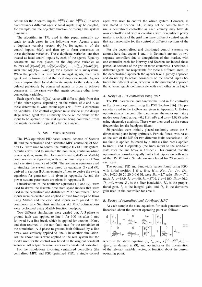
APPENDIX A

CALCULATING SWING PARAMETERS FOR GENERATOR 1

For the multiple HVDC link system in Fig. 1 the G, B, and

Y DC matrices are formed. The elements of Y DC are given by~di,j = dRi,j + jdIi,j . Taking equation (9) for generator 1 gives:

ωr1 =1

2H1

(

Pm1−G1,1E

′2q1−

E′

q1E

′

q4(G1,4 cos(δr1 − δr4) +B1,4 sin(δr1 − δr4))

+ g1,1PDC1 + g1,2P

DC2 −D1∆ωr1

)

(29)

The g1,1 and g1,2 parameters are derived as follows:

Assume that power flows from bus 2 to 1 in HVDC link 1

and from bus 3 to 4 in HVDC link 2:

IDC =

~IDC1,1

~IDC2,1

~IDC3,2

~IDC4,2

=

(PDC

1 −jQDC1

~U1

)∗

(−PDC

1 −jQDC1

~U2

)∗

(PDC

2 −jQDC2

~U3

)∗

(−PDC

2 −jQDC2

~U4

)∗

The generator power

PG1=R( ~Eq1

~I∗g1)

13

=R

(

~Eq1T ~Iq1

(

(G+ jB)E + Y DCIDC

)∗)

where T ~IG1

is a matrix of ones that picks out ~IG1. It is

the Y DCIDC part of this term that gives the g1,1 and g1,2parameters:

g1,1PDC1 + g1,2P

DC2

=R(

− ~EG1T ~IG1

(Y DCIDC)∗)

=R(

−~EG1

~U1

(dR1,1 + jdI1,1)∗(PDC

1 (1− jqr1))

−~EG1

~U4

(dR1,4 + jdI1,4)∗(PDC

2 (1− jqr2)))

where qr1 and qr2 are the ratios of reactive to active power in

HVDC links 1 and 2 respectively and δra,0 and θj0 denote the

initial conditions of the rotor angle of generator a and the bus

angle at bus j respectively. It should also be noted that the

complex~E~U

ratios are taken as constant in order to simplify

the equations. This process is then repeated for each generator.

APPENDIX B

POWER SYSTEM PARAMETERS USED IN THE SIMULATION

Sbase = 100× 106 VA, Ubase = 100× 103 V, fbase = 50 Hz,

w0 = 2πfbase rad/s.Line 1 2 3 4

XL pu 0.6 0.6 0.1 0.1

XS pu 0.1 0.1 0.1 0.1

Generator 1 2 3 4

x′

d pu 0.09 0.06 0.12 0.12

H (s) 2 4 2 2

D pu 1 1 1 1

PG = Pm pu 0.1 0.6 0.1 0.1

δr0 rad 5.9874 0.2871 5.585 5.03

E′

q pu 0.4454 0.513 0.6807 1.0622

Bus 1 2 3 4

Load pu 0.1+0.05i 0.1+0.05i 0.1+0.05i 0.6+0.2759i

U pu 0.1097 0.2426 0.256 0.2219

θ rad -0.4809 6.2768 5.5161 -1.3042

HVDC link a= 1 2

PDCa,0 pu 0.3573 0.1427

qra 0.8952 0.9037

APPENDIX C

PSO TOOLBOX PARAMETERS

The bounds for the optimisation of B, KP , KI ,

KD are: 0.01≤B14≤20, 0.01≤B32≤20, 0≤K14P ≤1000,

0≤K32P ≤1000, 0≤K14

I ≤10000, 0≤K32I ≤10000,

0≤K14D ≤1000, 0≤K32

D ≤1000. Parameters used for the

PSO Toolbox are given as follows:

Parameter Description

p number of particles 50

mvden max. velocity divisor 2

errgrad error gradient tolerance 1e-5

epoch maximum number of iterations 2000

errgraditernumber of epochs without errgrad

9change before termination