optimal corporate investments and capital...

Optimal Corporate Investments

and Capital Structure

2014-2

Martin Schultz-Nielsen

PhD Thesis

DEPARTMENT OF ECONOMICS AND BUSINESS

AARHUS UNIVERSITY � DENMARK

OPTIMAL CORPORATE INVESTMENTS AND CAPITAL STRUCTURE

Martin Schultz-Nielsen

A dissertation submitted to the

School of Business and Social Sciences, Aarhus University

in partial fulfillment of the requirements for the degree of

Doctor of Philosophy

in

Economics and Business

March 2014

3

Table of Contents

Preface

5

Summary

7

Chapter 1: Investing In Multiple Projects When The Firm Is Financially Constrained And Affected By Project Cash Flows

13

Chapter 2: Internal Financing In Financially Constrained Firms

49

Chapter 3: Liquidity And The Optimal Capital Structure 89

Dansk resume 139

5

Preface This dissertation is the result of my Ph.D. studies at the School of Business and Social Sciences at Aarhus University in the time period December 2009 to December 2012. I would like to thank the Department of Economics and Business at Aarhus University for providing excellent research facilities and generous financial support which has allowed me to attend numerous courses and conferences both in Denmark and abroad. This has all been made possible by the scholarship received from the Graduate School of Business and Social Sciences. I would like to thank my supervisors Professor Claus Munk and Professor Peter Ove Christensen for valuable guidance, feedback and encouragement. I would like to thank the faculty and the participants at the finance seminars for providing feedback on my work. Special thanks goes to Jens Riis Andersen and Christian Rix-Nielsen. I would also like to extend my gratitude to my fellow Ph.D. students for a friendly work environment and insightful discussions. Among others, these include Andreas Emmertsen, Jesper Wulff, Martin Klint Hansen, Manuel Lukas, Rasmus Varneskov and Rune Bysted. I am also thankful to Bibiana Paluszewska for proof reading my papers. I would also like to thank Boston University and Professor Jerome Detemple for the hospitality I enjoyed during my visit at the School of Management. This would not have been possible without the financial support from the Aarhus University Research Foundation and Knud Højgaards Fond. I would like to sincerely thank the members of the assessment committee, Associate Professor Stefan Hirth (Chair), Professor Carsten Sørensen and Professor Andrea Gamba, for their careful reading of this dissertation and their many insightful comments and suggestions. At last, but not least, I would like to deeply thank my family and friends for encouragement and support throughout the years. Martin Schultz-Nielsen Aarhus, March 2014

7

Summary This thesis consists of three self-contained chapters that all consider issues related to corporate finance. The three chapters are all driven by the same fundamental research question: How do cash flows generated by projects impact finance and investment decisions. Most corporate investment decisions are evaluated based on their expected value. An investment’s expected value is fundamentally connected to the cash flows it is expected to generate. The time-value of money means that early positive cash flows are valued higher than positive cash flows in the distant future. However, this thesis proposes that the timing of cash flows has a bigger impact than simply the time-value of money. The timing of cash flows affects how much funding is needed at different points in time. This affects both the project itself and other projects in the firm’s portfolio. The timing of cash flows becomes important because of imperfections in the capital markets. Transaction costs means that the firm has an incentive to minimize the use of the external financial markets. Asymmetric information and principal-agent issues between the firm and the capital markets can make it hard for some firms to acquire funding through these channels. It can also be hard if the firm or the owner is already indebted because of prior investments. This can be especially hard during times of crisis, where the amount of capital available in the economy is limited. A project that generates early positive cash flows and has a short payback period provides future investments with a cheap source of financing. This effect is not included in most valuation models, because they do not consider the dependencies that arise between current projects and future investment opportunities because of liquidity constraints. In practice, most firms correct for this by adjusting the cost of capital based on judgment. However, correctly adjusting the cost of capital requires that the adjustments are made dynamically over time, since it changes depending on the amount of liquidity and investment opportunities in the firm. This illustrates that properly accounting for the effect of liquidity is a complex task. This thesis analyzes how the effect of liquidity can be handled in a more rigorous manner. An analysis of the effect of liquidity can be split up into two parts: 1) How should a firm optimally invest and operate its projects when it is financially constrained, and 2) how should a firm optimally finance itself

8

given the liquidity needs of its projects. These two aspects are the focus of the three chapters in this thesis. Chapter 1 analyzes how a firm should optimally invest in projects, when it cannot acquire more financing than it has already acquired. Related papers analyze the effect of liquidity constraints for firms that have a single investment option. However, the most interesting dynamics arise when the firm has more than one investment option, since the investment in one project will affect the amount of cash available to other projects. Some papers do analyze this problem. However, none of these papers let the amount of liquidity be affected by the cash flows from operational projects. Since empirical evidence shows that most investments are financed with internal funds, this is an important dynamic. By incorporating this dynamic into our model, we find that the firm may invest in projects earlier than it would otherwise do, because it increases the probability that the firm can acquire enough cash to fund new projects before the opportunity is lost. We also find that the project’s cash flow profile is an important determinant when deciding on the optimal investment policy, since it affects whether the project can acquire enough liquidity to fund other projects. To compare the results to the related literature, we assume the firm cannot go bankrupt because of cash shortage, by assuming that the projects only generate positive cash flows once they are operational. This also allows us to develop a numerical method based on the Least-Squares Monte Carlo method which is very efficient, compared to if we allowed for negative cash flows. Chapter 2 extends the analysis from chapter 1, by allowing the cash flows to become negative, so the firm can go bankrupt because of cash shortage. Based on this analysis, we find that the cash flow profile is important even if the firm only has a single project, since it affects the probability that the firm will go bankrupt. We also find that the risk of bankruptcy makes the firm more inclined to wait for better market conditions, before it makes the investment. Some of this extra cautiousness will be offset, if the firm has the option to abandon the project once it is operational, because it can use the abandonment option to fight off bankruptcy. When the firm can invest in more than one project, we find similar results to those found in chapter 1. Cash flows from one project can be used to fund another project. However, the project’s cash flow profile becomes even more important with the risk of bankruptcy, because negative cash flows can now threaten the other projects in the firm’s portfolio. The profile of the other investment

9

options in the firm’s portfolio will therefore impact the value of each individual investment options. With multiple projects, we also find that the abandonment option can be used to the benefit of the other projects. The firm may therefore sell a project to fund other projects or save them from bankruptcy. Chapter 3 develops a model where capital structure decisions are centered around the firm’s liquidity needs, while still accounting for tax benefits, the cost of financial distress and collateral. Firms that incur external financing costs face a complex decision when they optimize the capital structure. Opportunity costs make it optimal to minimize excess cash in the firm, but transaction costs to raise funds means that cash should not be paid out too quickly. This means that the firm’s future liquidity needs must be accounted for when deciding on the optimal payments to equity holders and the optimal maturity structure and payment schedule for debt. We find that firms with cash cow projects will prefer to fund themselves with more debt than comparable firms. Because cash cow projects generate cash quickly, the firm can afford to pay bigger interest payments without having to seek further financing and pay transaction costs in the process. Firms will prefer debt types where the debt payment schedule can match the cash flows generated by the firm. If debt is paid back too slowly, it will lead to an excessive cash reserve being built up. Firms can reduce the probability of an excessive cash reserve being built up by choosing an appropriate schedule for debt payments or by choosing a short debt maturity, so the amount of debt can be adjusted dynamically. Firms will therefore optimize both the amount, type and maturity of debt to their liquidity needs. The model also allows us to analyze how the capital structure is affected when the firm can issue both long term and short term debt. We find that the firm prefers long term debt over short term debt as base capital, because it reduces the transaction costs over the firm’s lifetime. Short term debt is used to dynamically change the firm’s leverage over time, so the firm can flexibly increase its leverage in good conditions when additional debt financing is cheap. Together, these three chapters provide a comprehensive insight to the investment and financing decisions faced by a firm, when accounting for liquidity concerns. The models developed in this thesis are particular applicable to firms where liquidity management is important. An example of this are firms that for various reasons are capital constrained, e.g. if they are heavily indebted because of past bad investments or if the project

10

characteristics make it hard to acquire external financing. It is also the case for firms where there is a big difference in the size and occurrence of new investments. Such investments can have a big impact on the firm’s liquidity needs, which affects the optimal investment and financing policy. It is also particular applicable in times of crisis, where there is a limited amount of capital available in the economy. The credit crunch that arose during the financial crisis of 2008 showed that liquidity management can become important for even the most profitable firms.

INVESTING IN MULTIPLE PROJECTS WHEN THE FIRM IS FINANCIALLY CONSTRAINED AND

AFFECTED BY PROJECT CASH FLOWS

Martin Schultz-Nielsen* Department of Economics and Business

Aarhus University, Denmark

March 2014 Abstract Firms that are liquidity constrained will use cash flows from operational projects to fund future projects. The optimal investment policy will take this into account when deciding when and which projects to invest in. Where previous papers have only let liquidity be affected by the initial investment cost, this paper let liquidity be affected by the cash flows from the operational projects. We find that the firm may invest in projects earlier than it would otherwise do, because it increases the probability that the firm can acquire enough cash to fund new projects before the opportunity is lost. We develop a method which allows for a general specification of the cash flow process by extending the Least-Squares Monte Carlo method. We find that the firm will prefer to invest in projects which generate cash quickly, since it increases the probability that the firm can invest in additional projects.

Keywords: Multiple real options, Liquidity constraints, Least-Squares Monte Carlo JEL classification: C61, C63, D92, E22, G31, G32

14

1 Introduction The theoretical and empirical literature suggests that some firms are financially constrained and that the investment policy is affected by such constraints. Fazzari, Hubbard and Petersen (1988) provided empirical evidence that firm investments vary with the availability of internal funds. The models by Myers and Majluf (1984) and Greenwald, Stiglitz, and Weiss (1984) explain why asymmetric information between firms and capital markets can lead to market imperfections which can limit the firm’s use of external financial markets. Tirole (2006) also illustrate how principal-agent issues between management and investors can lead to capital market imperfections. The credit crunch that arose during the financial crisis of 2008 provided further evidence that sometimes firms can have trouble funding even the most healthy and profitable investments. According to Campello, Graham and Harvey (2010), 86% of U.S. CFOs in a sample of firms said their investments in attractive projects were restricted during the credit crisis of 2008. In this paper we analyze how a firm should optimally invest in new projects, given the financial constraints faced by the firm. A financial constraint will affect the optimal investment policy, since it constrains when and which projects the firm can invest in. The most interesting dynamics arise when the firm has more than one investment option, since the investment in one project will affect the amount of cash available to other projects. The analysis therefore focuses on the case where the firm has two investment options. An overview of the related literature shows that some papers analyze the effect of liquidity constraints in firms that have a single investment option. Some real option models analyze the effects and interactions that arise in firms with multiple investment options. A few papers do both, and incorporate a liquidity constraint in the analysis of multiple investment options. But none of these papers let the amount of liquidity be affected by cash flows from operational projects. In this paper we set forth to develop a model where cash flows from operational projects affect the amount of liquidity in the firm. Based on this model, we analyze the impact project cash flows can have on the optimal investment policy, given that the cash flows from one project can be used to fund the other project. Using data from the Federal Reserve, Brealey and Myers (2003, Chapter 14) show that more than 70% of the total financing of investments comes from internal financing. This shows that it is important to include the effects of project cash flows when deciding on the optimal investment policy. The seminal paper by McDonald and Siegel (1986) showed that a firm can maximize the value of an investment option by waiting for the right business conditions before investing. The literature on investment options is now vast and covers a myriad of different aspects and problems. Most papers assume that

15

funding is not a concern. However, a few recent articles have analyzed the consequences a liquidity constraint can have on the optimal investment policy. One of these is Boyle and Guthrie (2003), who extended the traditional McDonald and Siegel (1986) model by letting the amount of liquidity be stochastic, so the firm can become financially constrained. The problem analyzed by Boyle and Guthrie (2003) is restricted to one investment option, while we focus on the case with two investment options. However, because the amount of liquidity in Boyle and Guthrie (2003) is stochastic, it is possible to interpret the stochastic changes in the amount of liquidity as cash flows from an operational project. The investment problem in Boyle and Guthrie (2003) is therefore similar to the investment problem in this paper, after the firm has invested in the first project. Boyle and Guthrie (2003) find that the firm will have an increased incentive to invest in the project when the amount of liquidity is reduced. This is because the firm will prefer to make positive investments while it still can, instead of risking to lose the ability to make the investment because of insufficient cash. Our model can be modified to find similar results for the second investment option, after the firm has invested in the first project. Compared to Boyle and Guthrie (2003), this paper contributes with an analysis of the problem before the firm has invested in the first project. At this point, the firm must not only decide when to invest, it must also decide which of the projects to invest in. The analysis is interesting, because the liquidity constraint means that the projects become interdependent, and different tradeoffs must be analyzed when forming the optimal investment policy. First, the firm may have insufficient cash to invest in both projects at the same time, and the firm therefore has to make a relative assessment when deciding on which of the projects to invest in first. Second, the cash generated by the project can be used to fund the other project. This can impact when the firm should invest in the first project, since it can generate more cash the longer it has been operational. Investing in the first project early, may therefore increase the probability that it can generate enough cash to fund the other project. Gamba (2003) analyzed some of the option relationships that can arise between multiple investment options. Although he does not assume the firm is financially constrained, it is possible to make a comparison to these results. If the amount of liquidity in the firm is low, it may only be possible to invest in one of the projects. This corresponds to the mutually exclusive option relationship analyzed by Gamba (2003). In this option relationship, we find that the investment decision for each option becomes dependent on the state variable of the other investment option. This is because the investment decision should not just be based on the individual project value, but how valuable the project is relative to the other project. Such effects are not analyzed by Boyle and Guthrie (2003). We extend the

16

analysis of Gamba (2003) by allowing the amount of liquidity to be sufficiently high that the firm may be able to invest in the second project, although it is not guaranteed. Meier, Christofides and Salkin (2001) analyzed the interdependences that arise between multiple investment options when the firm is liquidity constrained. The constraint means that the firm can only invest in a subset of the possible projects. Similar to our paper, they find that the firm should not simply use the investment policies calculated for the investment options in isolation. This investment policy is suboptimal, since it disregards the value of the other possible projects. However, the model by Meier, Christofides and Salkin (2001) does not let liquidity be affected by the cash flows generated by the projects once they are operational. This means that the analysis is limited to how the firm should invest in the projects, given the constraint and the possible changes in the project values. By incorporating the cash flow dynamics, we can analyze how the firm’s investment policy is affected by the project’s cash flow profile, since this affects the firm’s ability to fund other projects. Brosch (2008) also analyze the problem where a firm with multiple investment options is subject to a liquidity constraint. Brosch (2008) allows the firm to acquire liquidity by disinvesting existing projects (i.e. exercising the option to abandon), so the firm can use the liquidity to invest in new projects. However, just like the previous models, cash flows from operational projects do not affect the amount of liquidity in the firm. For this reason, Brosch (2008) also cannot analyze how the project cash flows affect the investment decision when the firm is financially constrained. Letting liquidity be affected by project cash flows means that it becomes stochastic when the constraint is binding. This must be incorporated into the investment decision, and makes it difficult to solve using existing models. We build a framework based on the Least-Squares Monte Carlo (LSM) method, which is suited to solve these types of problems. We focus on the case where the firm has two investment options, and give a small overview of how the method can be extended to handle problems with multiple projects. By structuring the problem, we show that the problem can be seen as a choice between two possible option sequences. We show how the optimal investment policy can be calculated for each of the individual sequences, and how to choose between the two option sequences. The remainder of the paper is organized as follows. In Section 2 we analyze the simplified setting, in which we assume the firm must invest in the projects in a specific sequence. We set up the initial model, and develop a numerical method to

17

solve the model. We use the numerical method to calculate a set of results, which illustrate the dynamics of the model. In Section 3 we extend the model, so the firm is free to choose which of the projects it wishes to invest in first. This is followed by another set of results. Section 4 extends the specification of the cash flows, and illustrates how the cash flow profile affects the investment decision. Section 5 gives a small overview of how the model can be extended to more than two investment options. Section 6 concludes. A symbol list can be seen in Appendix B. 2 Initial model setup: A sequence of options In this section we set up the basic model, which we extend in the following sections. We assume the firm has two investment options, which gives the firm the option to invest in Project 1 and Project 2. In this section we assume that the firm can only invest in Project 2, after it has invested in Project 1. We will use this basic model structure in the following section, when we extend the model so the firm is free to choose which of the projects to invest in first. We set up the model for the problem, and construct a numerical method to solve the model. The numerical method is used to calculate a set of results, which illustrate the dynamics of the model.

2.1 Initial model

The model is based on the following assumptions. We assume time is discrete and break time into a number of periods with identical time increment !t. We let t denote the current time, and use h = {1,2} to denote each of the projects the firm can invest in. We assume the option to invest in each of the projects has maturity TIh, after which time it will be too late to invest in the project. Upon investment,

the firm must pay investment cost Ih. Once the investment is made, each project will have a lifetime of TP

h . While the projects are operational, they generate cash flows cft

h. The cash flows are dependent on state variable xth, which follows the stochastic process specified by !xth = !!xth!t + !!xth!zth ,! (1)

where !! is the drift, !! is the volatility and !zth is a Brownian motion. In this initial setup, we let xth denote the potential annual cash flow level once the project is operational. The realized cash flows will be dependent on when the firm invests in the projects. Let tsh denote the time the firm invests in the project h, where we in this section assume that ts1 < ts2. The project cash flows are then specified according to

18

!!cfth =

0 ! t < tsh

-Ih , t = tsh

xth ·!t , ts

h < t ! tsh ! TP

0 ! tsh ! TP ! !t

! (2)

where cft

h is the amount of cash generated in time increment !t. We let cft denote the total cash flows generated by the two projects, and let it be specified by cft = cft

1 ! cft2 .! (3)

Using these cash flows, the cumulative cash CCt generated by the projects can be calculated according to

CCt = cfs

t

s=0

!! (4)

The amount of cumulative cash generated (and used) by Project 1 affects whether the firm can invest in Project 2. The amount of liquidity is also affected by the funds acquired from external financing. For the purpose of clearly being able to determine value creation, we distinguish between liquidity received from operating and financing the firm. We denote liquidity received by financing the firm with B. We assume it is constant, and given by the amount of liquidity injected by the equity owner at time 0. For simplicity, we assume that all interests made on liquidity are paid out to the equity owner, but the model can easily be extended to allow for interests to affect the amount of liquidity in the firm. We assume there are no costs associated with holding liquidity, which is consistent with related literature, e.g. Boyle and Guthrie (2003). The variables are illustrated in Figure 1.

Figure 1

Illustration of the variables in the problem. Project cash

0 1 2 3 4 5 6

0.068

0.028

0.012

0.052

0.092

0.132

0.172

0.212

Cas

h flo

w

0 1 2 3 4 5 6

15

10

5

0

5

10

15

20

Cum

ulat

ive

cash

Time

Project 2 cash flow (L)Project 1 cash flow (L)Cumulative cash flow (R)

Ti

Tp

Liquidity constraint

19

flows are given on the left axis (L), cumulative cash on the right axis (R). The line illustrating the liquidity constraint is given by -B. The dashed lines before and after the cash flows illustrate the latent cash flows.

In Figure 1, the firm has an initial amount of financing of B = 15, while each project require an investment cost of Ih = 10. This means that the firm must wait for Project 1 to generate some cash, before it can invest in Project 2. The firm has to invest in the projects within TI

h = 2 years, or the investment options will be lost. Once the firm has made the investment, the project will be operational for TP

h = 4 years. In this specific example, the firm invests in Project 1 within the first few months. This reduces the amount of cumulative cash generated by the projects with the investment cost. The liquidity constraint is illustrated with a dashed line, set at !B. The firm cannot invest in a project if it leads to the amount of cumulative cash CCt falling below this dashed line, as it would correspond to the amount of liquidity in the firm becoming negative. Note, by assuming the project cash flows follow a GBM as specified by (1), we have implicitly assumed that the project cash flows will always be positive once the firm has made the investment. This means that the firm will not go bankrupt because of cash shortage after it has invested in the project. The dynamics that arise when allowing for bankruptcy are analyzed in Schultz-Nielsen (2013). The firm will invest in the projects with the objective of maximizing the total value of the investment options. Let the total value of the investment options be denoted by Ft, and let it be specified by

Ft xt1 ,!xt2!, CCt ! !t ! ! r ! s!t · cfs

1 ! cfs2

T

s=t

,! (5)

where T is the entire problem horizon, specified by T = max !TI1 ! TP1 !!!!!TI2 ! TP2 ! , and r is the annual risk free rate. Note, the total value of the portfolio of options is not equal to the sum of the individual option values when calculated based on a stand alone analysis. In this this section, it is partly because of the restriction that the firm can only invest in Project 2 after it has invested in Project 1. This reduces the value of the investment options. However, the liquidity constraint also reduces the value of the investment options, because the firm must accumulate the necessary liquidity before it can invest in Project 2. The optimal investment policy must account for this. The maximization problem is given by

maxts1!!!ts2!

Ft !,! (6)

where ts1 < ts2. Let Ft

h denote the value of the investment option for project h, given the restrictions, past decisions and the investment policy for the firm’s future

20

decisions. Let FtE,h denote the exercise value of the individual option, and let it be

specified by

FtE,h xt

h!!CCt

! !t 1 ! r - s!t ·cfsh

t+TP

s=t

!assuming!tsh ! t, if 0 ! B ! CCt

! if 0 ! B ! CCt

!!,!! (7)

for t ! TIh. The option can only be exercised if the firm has enough liquidity to invest in the project. Let Ft

C,h denote the continuation value of the individual option, and let it be specified by

FtC,h xt

1 ,!xt2!, CCt ! !t Ft+!th 1 ! r -!t !.! (8)

The continuation value will be dependent on the state variable for both projects. The investment option for Project 1 is affected by xt2, because it will impact whether or not the firm should prematurely invest in Project 1 to increase the probability of generating enough liquidity to invest in Project 2. Project 2 is dependent on xt1 because it affects the amount of cash flows Project 1 can generate, and whether it will be enough to accumulate the necessary liquidity in time to fund Project 2. When the firm has invested in Project 1, it will invest in Project 2 with the objective of maximizing the value of Project 2. This investment policy maximizes the total value of the investment options, because investing in Project 2 does not affect the value of operational Project 1. The value of the investment option for Project 2 is therefore given by

Ft2 xt

1!,!xt2 , CCt ! !"# !FtC,2!!! !FtE,2! !!when!!!ts1 ! t.! (9)

The investment will occur the first time the continuation value is no longer bigger than the exercise value of the investment option. This leads to the investment time specified by ts

2 = inf t ! 0!!t!! !TI2 : FtC!2 ! !FtE!2 !!when!!!ts1 ! t. ! (10)

If the investment event is triggered, the cash flows change as specified by (2). The investment policy for Project 1 is more complicated, since investing in Project 1 affects the investment option for Project 2. The firm cannot invest in Project 2 before it has invested in Project 1. This means that it may be optimal for the firm

21

to invest in Project 1 even though it has a negative exercise value, if the value of Project 2 is sufficiently high. This effect will be removed, when we in the following section allow the firm to freely choose which of the projects to invest in first. However, the liquidity constraint will still affect the decision of when to invest in the first project. It may therefore be optimal for the firm to invest in the project early, since this increases the time in which the project can generate cash flows which can be used to fund the second project. The optimal investment policy must account for this effect. We therefore calculate the total value from exercise FECt

1, which accounts for how the continuation value for the investment option for Project 2 is affected. The total exercise value from investing in the first project is specified by FECt

1 xt1!,!xt2!,!CCt ! FtE,1 xt1!,!CCt ! FtC,2 xt1!,!xt2!,!CCt ! I1 !!!! (11)

In calculating the continuation value for the Project 2 investment option, we must account for the reduction in the amount of liquidity caused by the investment in Project 1. Also note, that Ft

C,2 is not the continuation value for the investment option based on a stand alone analysis. It is the continuation value for the investment option given the restrictions, past decisions and the investment policy for the firm’s future decisions. The total exercise value must be compared to the total continuation value of waiting with the investment, FCCt. This is specified by FCCt xt

1!,!xt2!,!CCt ! FtC,1 xt1!,!xt2!,!CCt ! FtC,2 xt1!,!xt2!,!CCt !!!! (12) The firm will invest in Project 1 when the value from waiting with the investment is no longer higher the value from investing. This leads to the investment time specified by ts

1 = inf t ! 0!!t!! !TI1 : FCCt ! !FECt1 !. ! (13) If the investment event is triggered, the cash flows change as specified by (2), and the firm will invest in Project 2 as specified by (9) and (10).

2.2 Numerical method

To solve the model, we must calculate the values FtE,h, Ft

C,h, FECt1 and FCCt.

Because of the complexity of the problem, we construct a numerical method based on the Least-Squares Monte Carlo (LSM) method which can handle the necessary calculations. This section describes how the numerical method is set up. In the description we assume that TI = TI

1 = TI2, but the numerical method allows for TI

1 ! TI2.

22

We start by simulating N paths for xt1!and xt2, given the stochastic process specified by (1). We use ! ! {1, ... , N} to denote one of these simulated paths. Then we note that if the cash flows follow a GBM process as specified by (1), we can calculate the expected present value of the project cash flows using the calculation rules for geometric series. The stand alone value of investing in each of the projects, specified in (7), can therefore be calculated by

Ft!!E,h xt!!h !!CCt!!

! xt!!h !t 1 ! !h ! r !t 1 ! 1 ! !h ! r !t TPh!!t

1 ! 1 ! !h ! r !t , if 0 ! B ! CCt!!! if 0 ! B ! CCt!!

!,!!(14)

We will use this in the following subsections, when we set up a method that can calculate the remaining values.

2.2.1 Calculation of last period

The option values at time t depend on the expectations of the future and the investment policy for the future decisions. The numerical method must therefore be based on backward induction, and we start by making the necessary calculations for the last period, t = TI. For each simulated path !, we calculate the stand alone value of investing in Project 1 using (14), assuming t = TI and h = 1. At time t = TI, the value of the investment option Ft

2 for Project 2 will be zero, since the firm can only invest in Project 2 when Project 1 is operational. This means that the total value of investing in Project 1 is given by FECt!!

1 xt!!1 !,!xt!!2 !,!CCt!! ! Ft!!E,1 xt!!1 !,!CCt!! ! 0!!,! (15) assuming t = TI. Since this is the last possibility for the firm to invest in Project 1 before the investment option matures, we have that FCCt!! xt!!1 !,!xt!!2 !,!CCt!! ! Ft!!C,1 xt!!1 !,!CCt!! ! 0!!! (16) The firm will therefore invest in Project 1 for all of the simulated paths where the exercise value is positive. In the following iterations the numerical method will make the necessary calculations for each of the previous periods. In these calculations, we will have to calculate the continuation value of waiting with the first investment. For this purpose, we define the vector variables !1&2 and ts1!2. Let !1&2 ! be the actual present value of the future exercise decisions for every simulation !. Let ts1!2 !

23

be the optimal exercise time for the first investment in the sequence, given that it cannot be exercised before time t. In the last period t = TI, let it be specified by

ts1!2 ! ! t if 0 ! FECt!!1

! if 0 ! FECt!!1!.!! (17)

Given this specification of the starting time, let the optimal exercise value be given by

!1&2 ! ! 1 ! r - s!t ·cfs1

t+TP1

s=t

if t ! ts1!2 !

0 if t ! ts1!2 !

!,!! (18)

assuming t = TI. Note, that these optimal exercise values is what Longstaff and Schwartz (2001) denote as cash flows, and will form the basis for a least-squares estimation in the following subsection. !1&2 ! will include the present value of investing in Project 2, when it becomes possible and optimal for the firm to make the investment. Let !2 t,! denote the optimal exercise value for Project 2, assuming the firm has the necessary liquidity to exercise the investment option from time t. At time t = TI, the firm cannot invest in Project 2 because Project 1 is not yet operational, and the optimal exercise value is set to

!2 TI!! ! 0!.!! (19)

Let ts

2 t!! denote the optimal investment time, assuming the firm has enough liquidity to invest in Project 2, and that it cannot be exercised before time t. At t = TI, let it be given by

ts2 t!! ! !!.!! (20)

We will use ts

2 to calculate when it is optimal for the firm to invest in Project 2, after it has invested in Project 1.

2.2.2 Calculations for the second investment option

Once the calculations have been made for a specific period, the previous period is calculated. This is done for each period until time t = 0. First, we calculate the investment policy for Project 2 when we assume it has enough liquidity to exercise the option from time t. These calculations will be used to calculate the total value

24

of investing in the first project. To calculate the investment policy for Project 2 at time t, we first calculate the value of investing in Project 2, Ft!!

E,2. This is done using (14). Next, we calculate the continuation value Ft!!

C,2, based on the LSM method. As dependent variables we use the actual present values from waiting with the investment, calculated as the present value of the optimal future exercise values !2. We denote these actual values by Ft!!

C,2, and let it be specified by

Ft!!C,2

! 1 ! r ! ts2 t!!t!! !t ·!2 t!!t,! !.! (21)

Based on these actual values of the continuation value, we use the LSM method to calculate the expected continuation values Ft!!

C,2, by using basis functions based on xt!!2 . Based on this calculation, we update the optimal exercise value for period t by

!2 t,! ! 1 ! r - s!t ·cfs2

t+TP2

s=t

if Ft!!C,2 ! Ft!!E,2

!2 t!!t,! if Ft!!C,2 ! Ft!!E,2

!!.!! (22)

If it is not optimal to make the investment, we use the future optimal exercise value for the next period. The optimal investment time, when we assume the firm has enough liquidity to invest in Project 2, is calculated accordingly and specified by

ts2 t!! ! t if Ft!!

C,2 ! Ft!!E,2

ts2t!!t!! if Ft!!

C,2 ! Ft!!E,2!.!! (23)

Based on these calculations for Project 2, we can calculate below when the firm should invest in Project 1, and based on this investment policy, when it will invest in Project 2.

2.2.3 Calculation of the exercise value for the first investment

To calculate when the firm should invest in Project 1, we start by calculating the total portfolio value from investing in Project 1. This total value will include the value of possibly being able to invest in Project 2. Let !t!!*,2 denote the first time the firm has enough liquidity to invest in Project 2, assuming the firm invests in Project 1 at time t. Let it be specified by

25

!t!!*,2 = inf s ! t!!t!! !TI : 0 ! B ! CCs!! ! I2 if 0 ! B ! CCTI!! ! I

2

! if 0 ! B ! CCTI!! ! I2 !! (24)

If the firm does not have enough liquidity by TI, it will never have acquired the necessary liquidity and !t!!*,2 is set to infinity. Using this first possible investment time, it is possible to calculate the actual total value FECt!!

1 of investing in Project

1. This is calculated as the present value of the cash flows for Project 1 and the present value of the optimal exercise value for Project 2, given the time when it has enough liquidity to invest in the project. This is specified by

FECt!!1 ! ! ! r - s!t ·cfs

1

t+TP1

s=t

! 1 ! r - ts2 !t!!*,2 !! !t ·!2 ts

2 !t!!*,2!! ,!! .! (25)

This value could also be calculated by evaluating when the firm has enough liquidity to invest in Project 2, and from this point on evaluate when the firm should invest in the project. Using !2 and ts

2 saves us from repetitious calculations and makes the method more efficient. As FECt!!

1 are the actual values for the specific simulations, we use the LSM-

algorithm to ensure non-anticipativity. As a first step, we find the set of coefficients at that minimize the error in Least-Squares estimation specified by

at = argminaj,t

aj,t·Lj xt!!1 !,!xt!!2M

j=1

!FECt!!1

2N

! = 1

!,! (26)

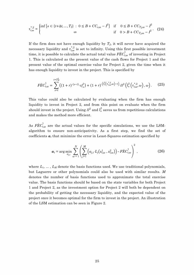
where L1, ... , LM denote the basis functions used. We use traditional polynomials, but Laguerre or other polynomials could also be used with similar results. M denotes the number of basis functions used to approximate the total exercise value. The basis functions should be based on the state variables for both Project 1 and Project 2, as the investment option for Project 2 will both be dependent on the probability of getting the necessary liquidity, and the expected value of the project once it becomes optimal for the firm to invest in the project. An illustration of the LSM estimation can be seen in Figure 2.

26

Figure 2

Illustration of the estimation of the total exercise value from investing in the first option at t = 0.33. The black circles indicate the point estimates of the exercise value, while the grey surface represents the LSM estimation based on the point estimates.

Given the coefficients at, it is possible to calculate an estimate of the total exercise value FECt!!

1 from investing in Project 1. This is calculated by

FECt!!1 = aj,t·Lj xt!!1 !,!xt!!2

M

j=1

!,! (27)

for each simulated path !.

2.2.4 Calculation of the value from waiting with the first investment

The total value from exercise must be compared to the total value from waiting with the investment, FCCt!!. !1&2 ! represents the actual optimal future exercise values. Based on these values we can calculate the point estimates for the continuation value, by discounting the future exercise values. This is calculated as

FCCt,! ! 1 ! r - ts1&2 ! !t ·!1&2 ! !,! (28) where ts1!2 ! is the future optimal investment time for Project 1. Based on these actual values from waiting with the investment, we must calculate the expected values to ensure non-anticipativity. We do this by finding the set of coefficients bt that minimize the error in the Least-Squares estimation specified by

bt = argminbj,t

bj,t·Lj xt!!1 !,!xt!!2M

j=1

!FCCt!!

2N

! = 1

! !! (29)

27

Based on these coefficients we calculate the expected value from waiting with the investment by

FCCt!! = bj,t·Lj xt!!1 !,!xt!!2M

j=1

!.! (30)

Note, that FCCt!! and bt are dependent on t, and change over time as the investment option approach maturity. The estimation for a specific period is illustrated in Figure 3.

Figure 3

Figure 4

Illustration of the estimation of the total value of waiting with the investment in Project 1 for the sequence of options at year t = 0.33. The black circles indicate the point estimates on the continuation value, while the white surface represents the LSM estimation based on the point estimates.

Illustration of the exercise decision of whether or not to invest in Project 1 at year t = 0.33, when the firm can only invest in Project 2 after it has invested in Project 1.

Based on these calculations of the total value of investment and the total value of waiting, it is possible to evaluate whether or not the firm should invest in Project 1 at time t. Given these calculations we update the optimal investment time by

ts1!2 ! ! t if FCCt!! ! FECt!!1

ts1!2 ! if FCCt!! ! FECt!!1

!,!! (31)

so the optimal investment time is updated if it is optimal to make the investment. Otherwise, the future optimal investment time is kept. The exercise decision is illustrated in Figure 4. Given this specification of the starting time, the future optimal exercise value is updated accordingly, so

!1&2 ! ! FECt!!1

if t ! ts1!2 !!1&2 ! if t ! ts1!2 !

!.!! (32)

28

We use these optimal future exercise values to calculate the value of waiting with the investment in (28). These calculations are done for every period back to time t = 0. Once this is completed, it is possible to calculate the total value of the investment options at time t = 0 as

F0 !1N

1 ! r - ts1&2 ! !t ·!1&2 !N

!=1!.! (33)

This is calculated for the optimal investment times as specified by (6).

2.3 Parameters

The results in this paper will be calculated based on the parameters specified in Table 1.

Table 1 Parameter values

Variables

"t 1/24 !1 = !2 -2% TI1 = TI

2 2 years !1 = !2 0.10 TP1 = TP

2 4 years I1 = I2 10 T 6 years B {10 , 15 , 20} r 3% N 200.000 x01 = x0

2 3

The time increment "t is set so the firm evaluates the decision of whether or not to invest two times a month. We assume the firm can invest in each of the projects for TI

1 = TI2 ! 2 years. Once the project is operational, they will be operational for

TP1 = TP

2 ! 4 years. We assume the risk free rate is r = 3%, and that the drift for the state variables is !1 = !2 ! -2%. We let the drift of the cash flows be negative, because we expect that the value of most investment options fall over time. This will either be because of the general technological progress or because competitors entrench their market position. The annual start level for the state variables is set to x0

1 = x02 ! 3, while the volatility is set to !1 = !2 = 0.10. We assume the

Brownian motions !zth for each of the projects are independent of each other. The investment cost is set to I1 = I2 = 10. The net present value for each of the projects is 0.86, upon investment at t = 0. A distribution for the possible cumulative cash generated by the projects can be seen in Figure 5.

29

Figure 5

Illustration of the distribution for the cumulative cash generated by each of the projects, when investing at time t = 0. Based on the parameters in Table 1.

The project initially requires a negative investment cost, after which point it generates positive cash flows. We analyze three cases, where the firm initially finances itself with B = 10, B = 15 and B = 20. The numerical method will be based on N = 200.000 simulated paths.

2.4 Results

In the initial model in this section, we have assumed that the firm can only invest in Project 2 after it has invested in Project 1. This corresponds to the compound option relationship analyzed by Gamba (2003). The compound option relationship analyzed by Gamba (2003) assumes that exercising an investment option gives the firm a payoff and another option. It does not account for liquidity constraints, and the only constraint is therefore that the firm must have invested in Project 1 before it can invest in Project 2. We denote this the option hierarchy. Gamba (2003) found that the optimal investment policy for the initial investment option will be affected by the compound option relationship. If the value of Project 2 is sufficiently high, it will be optimal for the firm to invest in Project 1, even though the net present value of Project 1 is negative. Otherwise, it would not be possible for the firm to realize the value of Project 2. Although the compound option relationship analyzed by Gamba (2003) does not account for financial constraints, it does find the optimal solution when B " 20. The firm will never be liquidity constrained for these amounts of financing, since the investment costs are Ih = 10 and the cash flows will be positive once the project is operational. For this reason, we can effectively disregard liquidity, and the model will find the same results as the compound option relationship analyzed by Gamba (2003). This is illustrated in Table 2.

0 0.5 1 1.5 2 2.5 3 3.5 410

8

6

4

2

0

2

4

Time

Cum

ulat

ive

cash

Expected cumulative cashCumulative cash percentiles 10%

90%

30

Table 2 Comparison of results for sequence of options for different amounts on financing

B = 10 B = 15 B = 20

Liquidity management

Option 1: 0.93 (75%)

Option 2: 0.00 (0%)

Total: 0.93 (0%)

Option 1: 0.85 (100%)

Option 2: 0.76 (57%)

Total: 1.61 (57%)

Option 1: 0.87 (97%)

Option 2: 0.91 (73%)

Total: 1.78 (73%)

Compound options

Option 1: 0.87 (97%)

Option 2: 0.91 (73%)

Total: 1.78 (73%)

Single option

Option 1: 0.93 (75%)

Total: 0.93 (0%)

Comparison of results for the sequence of options when the firm is financially constrained, to the results of compound options and the results for a single option when the firm is financially unconstrained. The percentages in the parentheses indicate how often the option was exercised, while the parentheses for Total indicates the probability that both options are exercised. The Single Option results are calculated using the traditional LSM-method from Longstaff and Schwartz (2001), and the Compound Options results are calculated using Gamba (2003). The Liquidity Management results are calculated using the numerical method described in this paper. Based on the parameters in Table 1. The computation time for the liquidity management model: B = 10: 6 min 15 sec, B = 15: 6 min 45 sec, B = 20: 14 min 20 sec. Computations were done on a Pentium Dual-Core 2.60GHz with 4 GB RAM.

From the table, we can see that the option values and exercise percentages are identical for the Compound Options model and the Liquidity Management model when B = 20. The Liquidity Management model is based on the model and numerical method developed in this section. For very low amounts of financing, the problem will approach another problem which has been analyzed before in the literature. If the amount of financing is so low that the firm will never be able to invest in Project 2, it is possible to regard the problem as a single option problem. As long as the firm has enough liquidity to make the investment in Project 1, it means that the effect from liquidity can effectively be disregarded. For B = 10, the firm will not be able to generate enough cash to invest in Project 2 within the two years the firm has the investment option. In Figure 5 we see that it takes the project more than 3 years to generate sufficient liquidity. This is confirmed by Table 2, where the exercise percentage for Project 2 is zero. For this reason, we also find that the option value and exercise percentage is identical to those found when solving the problem as a single investment option problem. The total option values for intermediate amounts of financing (B = 10 to B = 20) will be between the option values for these financing amounts, because no value can be lost by increasing the amount of financing or gained by decreasing it. However, for these intermediate amounts of financing it is necessary with a decision rule which specifically accounts for liquidity. This is because the investment decision for Project 1 will be affected by whether and when it can be expected to generate enough cash to fund Project 2. This is affected by the amount of financing acquired by the firm, which means that the optimal decision rule changes with amount B. Figure 6 illustrates the cumulative probability of

31

investing in Project 1, given the optimal decision rule, for different amounts of financing.

Figure 6

Illustration of the cumulative exercise probabilities for the investment option for Project 1, for different amounts of financing, for the liquidity management model described in this section. Based on the parameters in Table 1.

For B = 10 and B = 13, the firm will more less never be able to invest in Project 2, and the firm will therefore invest in Project 1 like it was a single option. For B = 15, we see a radical shift, and the firm will always immediately invest in Project 1. This amount of financing makes it sufficiently probable that Project 1 can generate enough cash to fund Project 2. However, it is also still so low, that the firm must invest in the project immediately, before it becomes too late for Project 1 to generate the necessary cash in time. For B = 17.5 more financing is acquired and the firm can wait before it becomes too late for Project 1 to generate the necessary cash in time. For B = 20 the firm is no longer liquidity constrained, and the firm will invest in Project 1 with the objective of maximizing the value of the compound options. 3 Model extension: Choice of initial option In the previous section we assumed that the firm had to invest in the projects in a specific sequence. In this section we extend the model, so the firm can choose which project to invest in first. This corresponds to the firm choosing a specific sequence, as illustrated by Figure 7.

0 0.2 0.4 0.6 0.8 1 1.2 1.4 1.6 1.8 20

0.1

0.2

0.3

0.4

0.5

0.6

0.7

0.8

0.9

1

Time

Cum

ulat

ive

exer

cise

pro

babi

lity

Financing, B = 10Financing, B = 13Financing, B = 15Financing, B = 17.5Financing, B = 20

32

Figure 7

We start by extending the model using the basic model structure developed in the previous section. Then we analyze how the numerical method can be extended to solve the model. This is followed by another set of the results.

3.1 Extension of model

In this section we extend the model from Section 2.1, so the firm can choose which of the project’s to invest in first. The structure of the model is the same as in Section 2.1, once the firm has invested in the first project. We therefore focus on the first investment decision. Similar to Section 2.1, the firm will invest when the total value from exercise is higher than the continuation value. However, the firm can now invest in both projects, so we start by finding which of the projects has the highest total exercise value. Let ht

! denote this project, and let it be specified by

ht! ! arg!max

hFECt

h xth! xtj !CCt !. (34)

The value for each FECt

h is specified as we did in (11), for each of the projects respectively. The firm will make the investment once the value from waiting is no longer higher than the value from investing. This leads to the investment time specified by ts

ht! = inf t ! 0!!t!! !TI

ht!

: FCCt ! !FECtht! !. ! (35)

Once the investment event is triggered, the cash flows change as specified by (2), and the firm will invest in the second project as specified by (9) and (10), by changing the project specification as required. Note, that the specification of the continuation value FCCt will be the same as in (12), but it will also be affected by the fact that firm can choose which of the projects to invest in first, and it will therefore be higher than in Section 2.1.

3.2 Extension of numerical method

We extend the numerical method so that it can solve the extended model. As with the model extension, we can use the same basic structure once the firm has

Portfolio of options

Option 1 Option 2

Choice

Option 2 Option 1

33

invested in the first project. The extension of the method is therefore focused on the choice of which project to invest in first, and how this affects the value from waiting with the first investment. The total exercise value FECt!!

h for each of the options is calculated as specified in Section 2.2.3. The continuation value FCCt!! is calculated as specified by (28), (29) and (30) in Section 2.2.4. However, the basis for the future optimal payoffs !1&2 in (28) will be different, as they will be modified to account for the fact that the firm can choose which projects to invest in first. First, we calculate which of the projects has the highest total exercise value for each of the simulations. Let this be calculated by

ht!!! ! 1 if FECt!!

1 ! FECt!!2

2 if FECt!!1 ! FECt!!2

!. (36)

Once the project with the highest total exercise value has been identified, it is possible to specify the optimal investment time by

ts1!2 ! ! t if FCCt!! ! FECt!!

ht!!!

ts1!2 ! if FCCt!! ! FECt!!

ht!!! !,!! (37)

where the investment time is updated if it is optimal to invest in one of the projects, and otherwise set to the optimal investment time calculated in the previous iteration. Given this specification of the starting time, the optimal exercise value can be calculated according to

!1&2 ! ! FECt!!ht!!!

if t ! ts1!2 !!1&2 ! if t ! ts1!2 !

!.!! (38)

This specification of the future optimal payoffs affects the continuation value FCCt!!, as !1&2 is now based on the possible initial exercise of both investment options instead of just one. The exercise decision is illustrated in Figure 8.

34

Figure 8

Illustration of the total exercise and continuation values from investing in the first project at year t = 0.333, when the firm is free to choose which of the projects to invest in first.

Compared to Figure 4, the figure also contains a plot of the total exercise value from investing in Project 2. The continuation value now increases more sharply with the state variable for Project 2, since the firm can invest in Project 2. With the given parameters, this leads to the effect that the firm will not necessarily invest in the project even though the state variable reaches a relatively high level. This is because it may be optimal to invest in the other project instead, if the state variable for the other project has a relatively high level. In this case it may be optimal for the firm to wait until one of the projects is clearly more valuable than the other. This effect is similar to the effect that can be found for options which are mutually exclusive. We analyze the similarities to this option relationship in the following subsection.

3.3 Results

In Section 2.4 we found that the problem will approach option problems which have been analyzed before for very low and very high amounts of financing. The same analysis can be done for the extended model. For low amounts of financing, neither of the projects may be able to generate enough liquidity to fund the other project. This means that the firm has to choose which of the projects to invest in, given that it cannot invest in the other as well. This corresponds to the Mutually Exclusive option relationship analyzed by Gamba (2003). When two options are mutually exclusive, only one can be exercised. In Table 3 we see that the option values and exercise percentages for the Mutually Exclusive Options model are identical to the option values and exercise percentages for the Liquidity Management model for B = 10, where the amount of financing is low.

35

Table 3 Comparison of results for different amounts of financing

B = 10 B = 15 B = 20

Liquidity management

Option 1: 0.70 (45%)

Option 2: 0.70 (45%)

Total: 1.40 (0%)

Option 1: 0.85 (72%)

Option 2: 0.85 (72%)

Total: 1.70 (47%)

Option 1: 0.93 (75%)

Option 2: 0.93 (75%)

Total: 1.86 (56%)

Mutually exclusive options

Option 1: 0.70 (45%)

Option 2: 0.70 (45%)

Total: 1.40 (0%)

Independent options

Option 1: 0.93 (75%)

Option 2: 0.93 (75%)

Total: 1.86 (56%)

Comparison of results for the investment options when the firm is financially constrained, to the results of mutually exclusive options and the results for independent options when the firm is financially unconstrained. The percentages in the parentheses indicate how often the option was exercised, while the parentheses for Total indicates the probability that both options are exercised. The Independent Options results are calculated using the traditional LSM-method from Longstaff and Schwartz (2001), and the Mutually Exclusive Options results are calculated using Gamba (2003). The Liquidity Management results are calculated using the numerical method described in this paper. Based on the parameters in Table 1. The computation time for the liquidity management model: B = 10: 8 min 27 sec, B = 15: 14 min 53 sec, B = 20: 33 min 20 sec. Computations were done on a Pentium Dual-Core 2.60GHz with 4 GB RAM.

For B " 20, the firm has enough liquidity that it can invest in each of the projects without having to wait for the other project to generate liquidity. The investment options are therefore independent of each other. The option values and exercise percentages for the Liquidity Management model for B = 20 are therefore the same as the option values and exercise percentages for the Independent Options model. In the Independent Options model, the decision rule for each of the investment options is calculated as if it was a single option, as we did in Table 2. For intermediate amounts of financing (B = 10 to B = 20), it is necessary to use the Liquidity Management model, because it may be optimal to invest in the first project earlier because of liquidity concerns, as we saw in Section 2. See Appendix A, for an illustration of how the total option value is dependent on the amount of financing B. 4 Modeling of cash flow profiles In the previous analysis we have assumed that the parameters for the two projects were identical. In this section we extend the specification of the cash flows, so each project can have a different cash flow profile. This allows us to model projects which have identical pre-investment project value dynamics, but where the expected timing of the cash flows can be different. We analyze how the cash flow profile affects the optimal investment decisions.

36

4.1 Model

We extend the specification of the cash flows in (2), so the cash flows become dependent on how long the project has been operational, and not just how much time has passed overall. The cash flow profile can be defined in a lot of ways, but to simplify the model we assume it is linear, and let it be specified by

!!cfth =

0 ! t < tsh

-Ih , t = tsh

!s0h+!h(t ! ts))xth ·!t , tsh < t ! ts

h ! TP0 ! ts

h ! TP ! !t

! !! (39)

where s0

h is the starting value and " is the annual incremental change. Such a specification of the cash flow profile is necessary, if the firm is free to choose when to invest in the project. If trying to adjust the cash flow profile through the starting value and drift of xth, we get some trivial solutions for the investment option; it will either be exercised immediately or as late as possible, depending on whether the drift for xth is sufficiently positive or negative. By letting the cash flow profile be dependent on the time the project has been operational, we are free to implement extremely increasing/decreasing cash flow profiles, without it correspondingly leading to pre-investment project values which are extremely increasing/decreasing over time. Using this specification of the cash flows, it is possible to use the same model and solution method specified in the previous sections.

4.2 Parameters

We use the parameters specified in Table 1. As parameters for the cash flow profile, we will model two different types of projects. The first project type will need to go through a stage of low cash flows before generating positive cash flows. We will call this type of project a growth project. The second project type generates positive cash flows from the beginning. However, these cash flows decline over time, and become low in the end. We will call this type of project a cash cow. We choose the parameters for the cash flow profile – the starting value s0h and the annual incremental change !h – such that the values of the two project

types are the same when the firm is liquidity unconstrained, and so the cash flows never become negative. Through calibration, we find the parameters specified in Table 4.

37

Table 4 Parameters for growth and cash cow project

Variable Growth project Cash cow

s0h 0.2 1.8

!h 0.4184 -0.4184 Parameters that are specific for the two project types.

With these parameters, the net present value of the project is 0.86 upon investment at t = 0, and the value of the single investment option is 0.93. This is identical to the values in Section 2.3. The value of the projects and individual investment options are therefore the same, and the only difference is the timing of the cash flows. Figure 9 and Figure 10 illustrate the distribution of the cumulative cash flows for the growth project and the cash cow project respectively.

Figure 9

Figure 10

Growth project: Illustration of the distribution for the cumulative cash generated by the growth project, when investing at time t = 0. Based on the parameters in Table 1.

Cash cow project: Illustration of the distribution for the cumulative cash generated by the cash cow project, when investing at time t = 0. Based on the parameters in Table 1.

In Figure 9, we can see that the amount of cumulative cash grows slowly in the beginning, but increases towards the end as the cash flow level increases. In Figure 10, we see the opposite, and the amount of cumulative cash grows quickly in the beginning, but the growth declines over time. In the following subsection, we analyze how the cash flow profile affects the optimal investment policy.

4.3 Results

The cash flow profile affects how fast the project generates cash. This will affect whether and when the firm can invest in the secondary project, which affects the optimal investment policy. We assume Project 1 is a growth project and Project 2 is a cash cow project. The value and exercise probabilities for B = 15 can be seen in Table 5.

0 0.5 1 1.5 2 2.5 3 3.5 410

8

6

4

2

0

2

4

Time

Cum

ulat

ive

cash

Expected cumulative cashCumulative cash percentiles

90%

10%

0 0.5 1 1.5 2 2.5 3 3.5 410

8

6

4

2

0

2

4

Time

Cum

ulat

ive

cash

Expected cumulative cashCumulative cash percentiles 10%

90%

38

Table 5 Results for projects with different cash flow profiles

B = 15

Liquidity management Option 1: 0.86 (64%)

Option 2: 0.88 (84%)

Total: 1.74 (52%)

Results for investment options on projects with different cash flow profiles. Project 1 is a growth project and Project 2 is a cash cow project. Based on the parameters in Table 1. The computation time for the liquidity management model: B = 15: 25 min 6 sec. Computations were done on a Pentium Dual-Core 2.60GHz with 4 GB RAM.

In Table 3 we saw that the value and exercise probabilities for the investment options were identical, when the cash flow profiles of the two projects were identical. In Table 5 we see that the value and exercise probabilities for the two investment options are different, when the cash flow profiles are different. We see that the firm will be more prone to invest in Project 2 when it is a cash cow project. Figure 11 illustrates the composition and timing of the total exercise probabilities for the two investment options. It illustrates the cumulative probability that the option is exercised as the first and second option respectively.

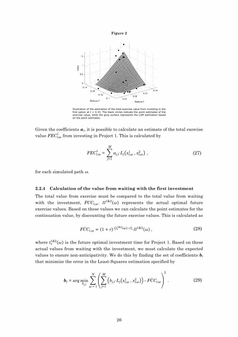
Figure 11

Cumulative exercise probabilities for the investment option on Project 1 and the investment option on Project 2, depending on whether it is the first or second investment. Project 1 is a growth project and Project 2 is a cash cow project. Based on the parameters in Table 1.

In Figure 11 we see that the investment option for Project 2, the cash cow project, is mainly exercised as the first investment. By investing in the growth project, it is unlikely that the firm can generate sufficient cash in time to invest in the second project. Vice versa, by investing in the cash cow project it is likely that the firm can invest in the second project, because the cash cow project generates cash quickly. This also means that the investment option for Project 1 is mostly exercised as a second investment, after the firm has invested in the cash cow project. This illustrates that a project’s cash flow profile will affect the value and optimal investment policy for an investment option.

0 0.2 0.4 0.6 0.8 1 1.2 1.4 1.6 1.8 20

0.1

0.2

0.3

0.4

0.5

0.6

0.7

0.8

0.9

1

Time

Cum

ulat

ive e

xerc

ise p

roba

bility

Option 1: First investmentOption 1: Second investmentOption 2: First investmentOption 2: Second investment

39

5 Extension to multiple project opportunities So far we have focused on the case with two investment options. In this section we review how the model can be extended to multiple investment options. Although a more elaborate problem structure is required, it is possible to decompose the problem using the basic model structures from Section 2 and Section 3. Figure 7 illustrated the model structure for two investment options. In Figure 12 we structure the problem for three projects using the same basic model structures.

Figure 12

Illustration of the model structure when the firm can invest in 3 projects.

From Figure 12 we can see that the firm initially has the choice between all three projects. This can be modeled in a similar fashion to what we did in Section 3.1. After the firm has invested in the first project, it can choose to invest in each of the remaining two projects. This subproblem is similar to the problem we analyzed in Section 3. This is represented by the dashed circles. By imagining that the dashed circles are in fact just options with complicated decision rules, we see that the problem structure is similar to the problem structure when the firm had two projects. The initial investment can therefore be seen as the choice of a sequence of options as before, and the only difference is that we have the choice between three projects instead of two. The same principle applies if considering even more projects, although the problem structure becomes even more complex. Although the problem can be structured in a similar manner to how the problem was structured in the previous sections, it also requires a minor extension of the numerical method. The required extension is related to the analysis concerning the second investment decision. In the previous analysis, we could use the calculations for the individual options once enough liquidity had been acquired.

Choice Portfolio of options

Option 1

Option 2 Option 3

Choice

Option 3 Option 2

Option 2

Option 1 Option 3

Choice

Option 3 Option 1

Option 3

Option 1 Option 2

Choice

Option 1 Option 1

40

However, with three projects, the firm can still invest in another project, and the optimal investment policy must account for this. Compared to the investment in the first project in the previous analysis, where the firm could also invest in another project, the difference is that it is no longer constant how much liquidity is available to the firm before the investment is made. The first project will generate cash, which makes the amount of liquidity in the firm stochastic. The numerical method in the previous sections assume that the amount of liquidity remains constant at this stage, and we therefore did not let the amount of liquidity affect the exercise or continuation values. By incorporating this is into the solution method, it is possible to solve the problem for multiple projects. The investment in the last project can be solved like in the previous sections, so it is based on the solution for the individual options once it has enough liquidity. One of the advantages of the Least-Squares Monte Carlo method is that the number of calculations only grows linearly with the number of state variables. With multiple investment options, we have to account for the interactions the projects can have on each other. This causes us to structure the problem as we have done in Figure 12. So although it is possible to solve the problem for multiple projects, we can see in Figure 12 that the problem quickly grows complex with the number of projects. In fact, it grows exponentially with the number of projects. Compared to the problem with 2 projects, the problem with 3 projects becomes at least four times as complex. For 3 projects, the problem can be decomposed into three 2-project-problems and an initial choice between the three options. For 4 projects, the problem becomes at least 17 times as complex. One possible way to reduce the complexity of the problem is by limiting the number of option sequences to include in the analysis. This can be done by excluding all of the possible option sequences which ex ante seem unlikely. This can greatly reduce the number of necessary calculations, so even problems with many projects can be solved. 6 Conclusion This paper has presented a general framework that can be used to calculate the value and optimal investment policy for a liquidity constrained firm which has two investment options. First, we analyzed the simplified setting where the firm had to invest in the projects in a specific sequence. Here, we found that the optimal investment policy corresponded to the investment policy for a single investment option, when the amount of financing acquired is so low that the firm can only invest in one project. When the amount of financing is so high that it can finance both projects, we found that the optimal investment policy is the same as for compound options when the firm is financially unconstrained. For intermediate amounts of financing, it is necessary with a model which specifically accounts for liquidity and the cash generated by the project when it is operational.

41

Accounting for liquidity will make the firm invest in the first project earlier, so the project can generate sufficient cash to fund the second project. After analyzing the simplified setting, we extended the analysis to when the firm is free to choose which of the projects to invest in first. When the firm has sufficient financing to invest in both projects, the optimal investment policy corresponds to the investment policy for two independent investment options. When the firm only has enough financing to invest in one project, the optimal investment policy corresponds to the investment policy for mutually exclusive options. The total value of the options will be in between these values for intermediate amounts of financing. Based on this model, we analyzed the effect a project’s cash flow profile can have on the optimal investment policy. We analyzed the optimal investment policy when the firm has a growth project and a cash cow project. We found that the firm prefers to invest in the cash cow project which quickly generates cash, because it increases the probability that the firm can invest in the second project. This illustrated that the cash flow profile is an important determinant when choosing which projects to invest in. Finally, we showed that the model can be extended to more than two projects using the basic model structure used for two projects.

42

References Boyle, Glenn W. and Guthrie, Graeme A., 2003, “Investment, Uncertainty, And Liquidity”, The Journal of Finance, Vol. 58, No. 5, pp. 2143-2166 Brosch, Rainer, 2008, “Portfolio Of Real Options”, Lecture Notes in Economics and Mathematical Systems, Springer Campello, Murillo; Graham, John and Harvey, Campbell, 2010, “The Real Effects Of Financial Constraints: Evidence From A Financial Crisis”, Journal of Financial Economics, Vol. 97, pp. 470-487 Harris, Milton and Raviv, Artur, 1996, “The Capital Budgeting Process: Incentives And Information”, The Journal of Finance, Vol. 51, No. 4, pp. 1139-1174 Fazzari, Steven; Hubbard, R. Glenn and Petersen, Bruce, 1988, “Financing Constraints And Corporate Investment”, Brookings Papers on Economic Activity 1, pp. 141–95. Gamba, Andrea, 2003, “Real Options: A Monte Carlo Approach”, Working Paper, forthcoming in Handbooks in Finance: Real Options by G.A. Sick and S. Myers (eds.), North Holland, accepted for publication. Greenwald, Bruce; Stiglitz, Joseph and Weiss, Andrew, 1984, “Informational Imperfections In The Capital Market and Macroeconomic Fluctuations”, The American Economic Review, Vol. 74, No. 2, pp. 194-199 Kulatilaka, N., 1995, “Operating Flexibilities In Capital Budgeting: Substitutability And Complementarity In Real Options”, Chapter 7 in “Real Options in Capital Investment – Models, Strategies, and Applications” by Trigeorgis, L., pp. 121-132 Longstaff, Francis A. and Schwartz, Eduardo S., 2001, “”Valuing American Options By Simulation: A Simple Least-Squares Approach”, The Review of Financial Studies, Vol. 14, No. 1, pp. 113-147 Meier, Helga; Christofides, Nicos and Salkin, Gerry, 2001, “Capital Budgeting Under Uncertainty”, Operations Research, Vol. 49, No. 2, pp. 196-206 Myers, Stewart and Majluf, Nicholas, 1984, “Corporate Financing And Investment Decisions When Firms Have Information That Investors Do Not Have”, Journal of Financial Economics, Vol. 13, pp. 187-221

43

Schultz-Nielsen, 2013, “Internal Financing In Financially Constrained Firms”, Working Paper Tirole, Jean, 2006, “The Theory Of Corporate Finance”, Princeton University Press Trigeorgis, Lenos., 1991, “A Log-Transformed Binomial Numerical Analysis Method For Valuing Complex Multi-Option Investments”, Journal of Financial and Quantitative Analysis, pp. 309-326 Trigeorgis, Lenos., March 1993, “The Nature Of Option Interactions And The Valuation Of Investments With Multiple Real Options”, Journal of Financial and Quantitative Analysis, Vol. 28, No. 1, pp. 1-20 !!

44

Appendix A Related to the results in Table 3, Figure 13 illustrates how the total value of the two investment options is dependent on B, the amount of liquidity acquired from financing.

Figure 13

Total option value calculated using the numerical method described in this paper. Based on the parameters in Table 1.

In Figure 13 we see that the added value from additional liquidity decreases with the amount of liquidity.

12 13 14 15 16 17 18 19 20 21 221.35

1.4

1.45

1.5

1.55

1.6

1.65

1.7

1.75

1.8

1.85

Liquidity from financing (B)

Valu

e

Total value of both options

45

Appendix B !t Size of the time increments t Current time h Used to denote a specific project TIh Years before the investment option matures Ih Investment cost TPh Project lifetime cfth Cash flow in time increment !t for project h at time t

xth State variable for project h at time t !! Drift for state variable !! Volatility for state variable !zth Brownian motion for state variable tsh Time the firm invests in project h

cft Total cash flows generated by the projects CCt Cumulative cash generated by the projects B Liquidity acquired from the equity holder Ft Total value of all the investment options T Entire problem horizon r Annual risk free rate Fth Value of the investment option for project h FtE,h Exercise value of the investment option for project h FtC,h Continuation value of the investment option for project h FECt

h Total value from exercising the investment option for project h as the first investment

FCCt The total value from waiting with the investment N Number of simulated paths used in the Monte Carlo simulation ! Specific simulated path !1&2 ! Actual present value of the future exercise decisions for both

investment options ts1!2 ! The optimal investment time for the first investment in the

sequence !h t,! The actual exercise value for project h, assuming the firm has the

necessary liquidity to exercise the investment option from time t tsh t!! The optimal investment time for project h, assuming the firm has

the necessary liquidity to exercise the investment option from time t

Ft!!C,h

The actual continuation value for the option for project h, based on the actual future exercise decisions.

!t!!*,h The first time the first has enough liquidity to invest in project h, assuming the firm invests in the other project at time t.

FECt!!h

The actual total value of investing in project h, based on the actual cash flows for the project and the actual future investment decision

46

for the other project. at Set of Least-Squares coefficients to calculate the total exercise

value FECt!!h .

L1, ... , LM Basis functions used in Least-Squares estimation. Here based on traditional polynomials.

M Number of basis functions used FECt!!

h Estimate of the total value of investing in project h for simulated path !.

FCCt,! The actual total continuation value of waiting with the first investment, based on the actual future investment decisions for the projects, and the actual cash flows.

bt Set of Least-Squares coefficients to calculate the total continuation value FCCt!!.

FCCt!! Estimate of the total continuation value of waiting with the first investment for simulated path !.

ht! Project with the highest total exercise value, FECt

h. ht!!! Project with the highest total exercise value, FECt

h, for simulated path !.

s0h Starting value for the cash flow profile with a linear specification. " Annual incremental change in the cash flow profile specification.

INTERNAL FINANCING IN FINANCIALLY CONSTRAINED FIRMS



March 2014 Abstract Empirical evidence suggests that some firms are highly dependent on internal financing because external financing is costly. This means that a project’s cash flow profile is an important determinant when choosing which projects to invest in and which to abandon. This paper develops a model that illustrates these effects. First, the paper shows that a firm’s cash flow profile is important if the firm only has a single project. If the firm does not have liquidity to finance operations it will be forced into bankruptcy. This will impact the firm negatively if the project was expected to generate positive cash flows in the future. This makes the firm more inclined to wait for better market conditions when it is financially constrained. Having the option to shut down or sell the project offsets some of this negative effect. When the firm has multiple projects, we see that cash from one project can be used to fund other projects. This means that a project which generates positive cash flows early, contributes with more value than an otherwise identical project. This effect has not been analyzed in previous papers. We also show that it may be optimal to sell an otherwise profitable project, when the funds can be used to finance another project.

Keywords: JEL classification: C61, C63, D92, E22, G31, G32

Martin Schultz-Nielsen, Department of Economics and Business, Building 2622, Aarhus University, DK-8000 Aarhus C, Denmark, [email protected]. The author would like to thank Carsten Sørensen, Claus Munk, Jerome Detemple, Peter Ove Christensen, Jens Riis Andersen and the participants of the Aarhus University Finance Seminars for helpful comments.

*

Liquidity constraints, Bankruptcy, Abandonment, Private risk,

Cash flow profile, Multiple real options, Least-Squares Monte Carlo

50

1 Introduction Firms face a lot of decisions regarding their ongoing projects and the optimal investment strategy. This reflects the many options and the amount of flexibility available to the firm in a world of constant change. The real option literature has developed a wide set of models and tools which can be used to valuate firms and guide them in their decisions. Two of the most analyzed traditional real options have been the investment option and the abandonment option. The traditional argument has been that it is optimal to delay investment until market conditions pass a certain threshold, and abandon it again if passes below another threshold. However, in this paper we propose that liquidity concerns may also impact the decision of whether or not to invest in or abandon a project. A firm which is liquidity constrained will take into account a project’s cash flow profile when deciding which project to invest in, because it may lead to bankruptcy if it runs out of cash. It may also choose to sell a project to raise liquidity to avoid bankruptcy. Such interdependencies between projects have not been analyzed by past real option models. The contribution of this paper is a model which can be used to analyze the value and optimal policy for a liquidity constrained firm, which has two investment options embedded with abandonment options. The model is used to illustrate the effect of the project’s cash flow profile. Some past models have analyzed the effect liquidity constraints can have on a single investment option. However, the most interesting effects arise when considering multiple projects, so that the cash flows from one project can limit or fund the investment of other projects. The seminal paper by McDonald & Siegel (1986) pointed out that there is value in optimally managing when to invest in a project, since market conditions change all of the time. Another important early contribution to this literature is Dixit and Pindyck (1994) who review several decisions that are at the company’s disposal. One of these is the option to abandon a project, which we incorporate in our model. This early literature all assume perfect capital markets and do not consider potential financial constraints. The review article by Hubbard (1998) finds empirical evidence that the cost of external and internal financing are not the same. This suggests that capital markets are in fact not perfect. Several papers suggest that these capital market imperfections can be due to asymmetric information or agency problems. While we will not try to explain why they exist, we accept that they do. Boyle and Guthrie (2003) examine the effect of a financial constraint on the timing and value of the traditional investment option. They assume the amount of liquidity is stochastic so the firm cannot be certain that it will have the necessary funds to pay the investment cost in the future. They conclude that the firm will be more prone to invest in the project when the firm’s liquidity is reduced. In this paper we reach the opposite conclusion. This is because we model the cash flows after the firm has invested in the project and

51

allow for potential bankruptcy. Meier, Christofides and Salkin (2001) examine the optimal investment strategy for a financially constrained firm with several investment options. Since the values of the different investment options evolve differently over time, it is not optimal to select the options that have the highest value from the outset and disregard the rest. They assume that the amount of cash is only affected by the investment cost, and like Boyle and Guthrie (2003) they do not consider bankruptcy or model the cash flows after the firm has invested in the project. For this reason they cannot show how cash flows from one project can be used to finance other projects as we do in this paper. The remainder of the paper is organized as follows. In Section 2 we set up the basic model for a single investment option. We illustrate how the project’s cash flow profile affects the project’s value and investment threshold. Section 3 extends the model, so the firm can also abandon the project once it is operational. We illustrate how this affects the value, investment threshold and risk of bankruptcy. In Section 4 the model is extended to two investment options with embedded abandonment options. The results show how the cash flows from one project is used to finance the other, and how the cash flow profile of the two projects affects the value of the firm. Section 5 concludes. Appendix B gives an overview of the variables used. 2 Investment option This section sets up the initial model and illustrates the dynamics of the investment option for a single project. We specify how the cash flows are given, and the effects of bankruptcy. This is followed by results which illustrate the effects of the cash flow profile. We assume the firm has no options at its disposal after it has invested in the project.

2.1 Model

The model is based on the following assumptions. We assume time is discrete and break time into a number of periods with identical time increment !t. The firm has an investment option, which gives it the opportunity to invest a project until time TI. Upon investment, the firm must pay investment cost I. The resulting project has a lifetime of TP, in which time it generates after tax operating cash flows cfot. Denote the total problem horizon as T = TI + TP. The cash flows are dependent on state variable xt, which follows the stochastic process specified by !xt = µxt!t + !xt!zt ,! (1)

where µ is the drift, ! is the volatility and !zt is a Brownian motion. The operating cash flows will be dependent on when the firm invested in the project

52

and whether the firm has gone bankrupt. Let ts denote the time the firm invests in the project and tb the time the firm goes bankrupt. The project cash flows are then specified according to

!cfot =

0 ! t < ts-I , t = ts

!!s0+!(t ! ts))xt – fc)·!t , ts < t ! min ts ! TP!! tb0 ! min ts ! TP!! tb ! !t

!,!! (2)

where fc denotes the annual fixed costs. The contribution margin is dependent on xt and a set of variables that specify the cash flow profile. The cash flow profile affects the cash flows depending on how long the project has been operational (contrary to how much time has passed overall) and is therefore dependent on the investment time ts. The cash flow profile can be defined in a lot of ways, but to simplify the model we assume it is linear. Let s0 denote the starting value, and " the annual incremental change. Such a specification of the cash flow profile is necessary, if the firm is free to choose when to invest in the project. If trying to adjust the cash flow profile through the starting value and drift of xt, we get some trivial solutions for the investment option; it will either be exercised immediately or as late as possible, depending on whether the drift for xt is sufficiently positive or negative. By letting the cash flow profile be dependent on the time the project has been operational, we are free to implement extremely increasing/decreasing cash flow profiles, without it correspondingly leading to pre-investment project values which are extremely increasing/decreasing over time. The above variables specify the project cash flows. However, the firm’s liquidity is also affected by the funds it acquires from external financing. For the purpose of clearly being able to determine value creation, we distinguish between liquidity received from operating and financing the firm. We denote liquidity received from financing the firm by B. We assume it is constant, and given by the amount of equity injected by the owner at time 0. We let the amount of cumulative cash generated by the firm be given by CCt. The cash flows from financial activities cfft consists of the return on the firm‘s liquidity. We assume the liquidity is placed in a money market account with risk free interest rate r, so that

cfft ! B ! CCt!!t ·r·!t .! (3)

The firm’s total cash flows are made up of these two cash flow streams: cft ! cfft ! cfot .! (4)

It is these cash flows which make up the amount of cumulative cash CCt, calculated as

53

CCt = cfs

t

s=0

!! (5)

The amount of cumulative cash generated by the firm will impact when and if it goes bankrupt. In Leland (1994) and related papers, bankruptcy is an endogenous decision. In this paper, bankruptcy is an event that is triggered when the total amount of cash in the firm is negative. It is therefore not a control variable. However, in the following section the firm will be allowed to abandon the project, which is comparable to liquidation of the firm even if it has sufficient liquidity. We assume bankruptcy leads to the firm being shut down, so it can only happen once. Bankruptcy therefore occurs the first time the total amount of cash in the firm is negative, specified by tb = inf t!!! 0!!t!! !T !: CCt + B < 0 .! (6) This event leads to the firm being shut down and changes the cash flows as specified by (2). The firm will invest in the project with the objective of maximizing the value of the firm. Let the firm value FVt be defined as the value of the accumulated liquidity and the expected present value of the project cash flows,

FVt xt , CCt ! !! ! ! r - s!t ·cfosT

s!t! CCt-!t ! B ! cfft ! !! (7)

Let Ft denote the value of the investment option, specified as the expected present value of the future project cash flows given optimal investment time ts. When the firm has a single investment option, the firm value can be rewritten to

FVt xt , CCt ! Ft ! CCt-!t ! B ! cfft .! (8)

This implies that firm value is maximized by maximizing the value of the investment option. McDonald & Siegel (1986) showed that a firm can maximize the value of an investment option by waiting to exercise the option until the right time. The maximization problem is specified by

maxtsFVt!.! (9)

The optimal investment policy is to exercise the investment option when the exercise value of the option is higher than the option’s continuation value. The exercise value of investing in the project today, Ft

E, is specified by

54

FtE xt , CCt ! !! ! ! r - s!t ·cfos

t+TP

s!tassuming ts ! t!.! (10)

Note, compared to the traditional investment option in McDonald & Siegel (1986), the option here is also dependent on the amount of cumulative cash CCt. This is because CCt affects the probability of bankruptcy, which affects the value of the project through (2). The continuation value from waiting with the investment is the expected present value of the investment option in the next period. This corresponds to the value of the future cash flows, when the firm is free to choose the future investment time. The investment option’s continuation value is specified by

FtC xt , CCt ! !t Ft+!t 1 ! r -!t !.! (11)

Maximization of the objective function means the firm makes the decision which contributes to the highest value until the firm invests in the project. The value of the investment option is therefore specified by !Ft xt , CCt ! max Ft

C!!!!!!!FtE for t ! ts .! (12)

The investment will occur the first time the continuation value is less or equal to the exercise value of the investment option. This leads to the investment time specified by ts = inf t ! 0!!t!! !TI : Ft

C ! !FtE . ! (13) Once the investment event is triggered, the cash flows change as specified by (2).


In the following sections we will extend the model, and give the firm the opportunity to abandon the project and the opportunity to invest in another project. The second investment option will be based on a separate state variable. The optimal decisions are conditional on the state and actions taken with respect to both projects. Simply having two investment options with embedded abandonment options can lead to many possible scenarios and interdependencies as illustrated by Figure 12. This can be hard to handle for many numerical methods if we want the projects to be non-identical. We find that a framework can be built using the Least-Squares Monte Carlo (LSM) method by Longstaff & Schwartz (2001) which can be used to solve such complex problems. The numerical method for the model in this section is very similar to the traditional

55

LSM method. The model in this section can most likely also be solved using the finite difference method (although no real options papers have been found which account for the accumulated cash generated by the project). However, the method described here will be the core of the method which we will extend in the following sections. It would be difficult to solve the extended model with the finite difference method. The numerical method starts by simulating a set of paths for state variable xt. Through backward induction starting at time TI, the method calculates the actual values of investing in the project today and of waiting with the investment. The future decision rules needed to calculate the value of waiting with the investment are based on the calculations from the previous iterations. The values are calculated by discounting the cash flows, which are calculated as specified according to (2). Compared to a traditional investment option, we also account for the fact that the firm can go bankrupt if the total amount of cash in the firm becomes negative. The actual values of investing and waiting with the investment are used as dependent variables in a least squares estimation. As independent variable we use basis functions based on state variable xt. With the coefficients from the least squares estimation we can calculate the expected value of waiting and investing in the project, which is used to make the investment decision.

2.3 Parameters

In this analysis we will use two different types of projects to illustrate the effects of the cash flow profile. The first project type will need to go through a stage of negative cash flows before generating positive cash flows. We will call this type of project a growth project. The second project type generates positive cash flows from the beginning. However, these cash flows decline over time, and may become negative in the end. We will call this type of project a cash cow. We choose the parameters for the cash flow profile – the starting value s0 and the annual incremental change " – such that the values of the two project types are the same when the firm is liquidity unconstrained. The parameters that are common for both project types are specified in Table 1. We assume the firm can invest in the project for TI = 2 years, after which time the opportunity will be lost. After investing, the project will have a lifetime of TP = 4. Investing in the project requires investment cost I = 10. The annual start level for the state variable is set to x0 = 12. Because of the general technological progress, we assume the state variable has a negative drift of µ = -2%, and that the volatility of the state variable is ! = 0.20. The annual fixed costs are set to fc = 8. We set the amount of initial equity financing to B = 12.

56

Table 1 General parameters

Parameters Parameters

TI 2 x0 12 TP 4 µ -2% I 10 ! 0.20 B 12 fc 8 r 3% !t 1/24

Parameters that are common for the two types of projects.

The parameters for the two project types are specified in Table 2.

Table 2 Parameters for growth and cash cow project


s0 0.2 1.8 " 0.4 -0.4366

Parameters that are specific for the two project types.

The net present value for each of the two projects when investing at time t = 0 is equal to 1.8 when the firm is liquidity unconstrained. The value of the investment option (where the firm is free to choose at which time to invest in the project) is in both cases equal to 4.6 when the firm in liquidity unconstrained. The distribution of the operating cash flows cfot and the resulting cumulative cash flows are illustrated in Figure 1 and Figure 2 for the growth project and Figure 3 and Figure 4 for the cash cow.

Figure 1

Figure 2

Distribution of annual operating cash flows, cfot, for growth project when the firm is unconstrained, and project is started at time 0.

Distribution of the cumulative cash from operating cash flows for growth project when the firm is unconstrained, and project is started at time 0.

0 0.5 1 1.5 2 2.5 3 3.5 4 4.50.4

0.2

0

0.2

0.4

0.6

0.8

1

Time

Year

ly c

ash

flow

leve

l

Cash flow percentiles

80%

90%

70%

60%50%

20%

10%

30%40%

0 0.5 1 1.5 2 2.5 3 3.5 4 4.520

15

10

5

0

5

10

15

20

25

Time

Cum

ulat

ive

cash

Cumulative cash percentiles 90%

50%

80%

70%

60%

40%30%

20%

10%

57

Figure 3

Figure 4

Distribution of annual operating cash flows, cfot, for cash cow project when the firm is unconstrained, and project is started at time 0.

Distribution of the cumulative cash from operating cash flows for cash cow project when the firm is unconstrained, and project is started at time 0.

We assume the firm makes decisions two times a month, so the time increments have a size of !t = 1/24. The calculations are based on 200.000 simulations, and as polynomials for the basis functions we use standard polynomials up to order 3 or 4 depending on the variable, and use cross-polynomials where it has been found optimal. Appendix A gives an estimate of the precision of the model for the basic problem, by comparing it to other numerical methods. Using these parameters, we move on to the results.

2.4 Results

The parameters have been chosen so that the value of the two project types are the same when the firm is liquidity unconstrained. However, when the firm is liquidity constrained, we find that the cash flow profile will affect the value and investment threshold of the investment option. The results for the investment option for the two different projects types are given in Table 3.

Table 3 Results for investment option


FV0 - B 3.1 4.5 Bankruptcy probability 20.8% 0.2% Investment probability 23.8% 57.1% Expected inv. time 1.7 1.1

Results for initial equity financing B = 12.

The cash flow profile affects the probability of whether and when the firm will run out of cash and go bankrupt. In Table 3 we can see that the probability of bankruptcy is 0.2% for the cash cow project and 20.8% for the growth project. In Figure 5, we see that the firm with the growth project almost runs out of cash and

0 0.5 1 1.5 2 2.5 3 3.5 4 4.50.4

0.2

0

0.2

0.4

0.6

0.8

1

Time

Year

ly c

ash

flow

leve

l


90%

70%80%

10%20%30%40%50%60%

0 0.5 1 1.5 2 2.5 3 3.5 4 4.510

5

0

5

10

15

20

Time

Cum

ulat

ive

cash

Cumulative cash percentiles

10%

20%

30%

50%40%

60%

70%

80%

90%

58

goes bankrupt, while the firm with the cash cow project in Figure 6 generates plenty of cash.

Figure 5

Figure 6

Illustration of investment decision and cash flows for the growth project. Project cash flows are on the left axis (L), and cumulative cash on the right axis (R).

Illustration of investment decision and cash flows for the cash cow project. Project cash flows are on the left axis (L), and cumulative cash on the right axis (R).

This affects the value of the investment option, so the value of the cash cow investment option is 4.5 while the value of the growth project investment option is 3.1. To maximize the value of the investment option, the firm optimizes the investment decision with respect to the cash flow profile of the firm. This means that the firm is less likely to invest in the project when the project is a growth project than when it is a cash cow, because the increased probability of bankruptcy makes it less likely that the investment will be profitable. This means that the firm will only invest in the project when conditions are good, i.e. for high values of the state variable. In Table 3 we can see that this decreases the probability that the firm will make the investment from 57.1% to 23.8% and delays the expected time of investment from 1.1 years to 1.7 years, compared to when the project is a cash cow. Including the effect of bankruptcy, leads us to results which are contrary to those found in Boyle and Guthrie (2003). Boyle and Guthrie (2003) conclude that the firm is more likely to exercise the investment option when the firm has a low level of liquidity. This is done under the assumption that the firm cannot go bankrupt, so the firm can effectively disregard the liquidity constraint after it has made the investment. Figure 7 illustrates how the exercise boundary in our model depends on the initial amount of liquidity when the project is a growth project. By including the possibility of bankruptcy, Figure 7 illustrates that the exercise boundary increases for decreasing amounts of initial liquidity.

0 1 2 3 4 5 6

0.2166

0.0567

0.1032

0.2631

0.423

0.5828

0.7427

0.9026

Cas

h flo

w

0 1 2 3 4 5 6

15

10

5

0

5

10

15

20

Cum

ulat

ive

cash

flow

Time

Project cash flows (L)Cumulative cash flows (R)

B

Cash flow start level

0 1 2 3 4 5 6

0.2166

0.0567

0.1032

0.2631

0.423

0.5828

0.7427

0.9026

Cas

h flo

w

0 1 2 3 4 5 6

15

10

5

0

5

10

15

20

Cum

ulat

ive

cash

flow

Time

Project cash flows (L)Cumulative cash flows (R)

B

Cash flow start level

59

Figure 7

Exercise boundary for investment option, both in relation to what level the state variable should attain (left axis (L)) and what the project value should be (right axis (R)). Exercise boundary at t = 1.83.

The exercise boundary with respect to the state variable and the exercise boundary with respect to the project value are not completely aligned in the figure. This is because both the investment decision and the project value are affected by the amount of liquidity available. This leads to two opposing effects on the project value exercise boundary. More liquidity will on the one hand make bankruptcy less likely, and therefore encourage the firm to invest at lower levels of the project value. On the other hand, we also have that the project value will increase when the probability of bankruptcy is reduced. This effect may not change monotonically with the amount of liquidity, which can cause some misalignment between the two exercise boundaries. The cash flow profile affects how much external financing the firm should raise to get the most value out of the project. The growth project requires more financing than the cash cow which generates cash flows from the beginning. The relationship between the net firm value and the liquidity raised can be seen for both project types in Figure 8 and Figure 9. We compare these values to the value of the simple investment option, when the firm is financially unconstrained and cannot go bankrupt.

11 12 13 14 15 16 17 18 19 20

0.5265

0.5666

0.6067

0.6468

0.6868

0.7269

0.767

0.8071

Initial equity financing

Stat

e va

riabl

e le

vel

State variable exercise boundary (L)Project value exercise boundary (R)

11 12 13 14 15 16 17 18 19 20

6

8

10

12

14

16

18

20

Proj

ect v

alue

leve

l

60

Figure 8

Figure 9

Growth project. Net firm value, FV0-B, for different amounts of initial liquidity, when the company can go bankrupt and when it cannot.

Cash cow project. Net firm value, FV0-B, for different amounts of initial liquidity, when the company can go bankrupt and when it cannot.

Comparing the two figures we see that the growth project is dependent on the firm having the necessary liquidity to bring the project to the stage where it generates positive cash flows. The cash cow needs the bare minimum of liquidity. This illustrates that the investment option is dependent on the amount of liquidity available and the cash flow profile of the project, and it is therefore relevant to develop a model which takes such liquidity concerns into account. 3 Abandonment option In Section 2 we assumed the firm had no possible actions at its disposal after it invested in the project. In this section we extend the model and allow the firm to abandon the project. There are two ways in which the firm can abandon the project. It can close down the project or it can sell the project. There may be costs associated with closing down the project, e.g. benefits to employees. However, it may be optimal to close down the project if the value of keeping the project running is negative. If the project still has value, it may be optimal to sell the project instead of closing it down. We assume the project has a salvage value which is dependent on the market conditions. The firm will sell the project when the salvage value is higher than the value of keeping the project. This occurs when the firm is low on liquidity and the threat of bankruptcy decreases the value of the project. In this case it is better to let the project be acquired by another firm which has the necessary liquidity to finance the project through the stage of negative cash flows.

11 12 13 14 15 16 17 18 19 200

0.5

1

1.5

2

2.5

3

3.5

4

4.5

5

5.5


Net

firm

val

ue

Gro

wth

pro

ject

No bankruptcyBankruptcy

11 12 13 14 15 16 17 18 19 200

0.5

1

1.5

2

2.5

3

3.5

4

4.5

5

5.5


Net

firm

val

ue

Cas

h co

w p

roje

ct

No bankruptcyBankruptcy

61

3.1 Model setup

We extend the model from Section 2 to include the option to abandon the project once it is operational. Assume the time of abandonment is given by ta, and that ts < ta. This changes the maximization problem so it is now specified by

maxts ! ta

FVt !.! (14)

The firm still invests in the project using the decision rules specified in Section 2. However, the investment decision is affected by the firm’s option to abandon the project. The decision rule related to the abandonment option is dependent on the present value of the project once it is operational. To calculate the project value once it is operational, we introduce p to denote the time the project has been operational. This is given by p ! t ! ts .! (15)

This leads to the calculation of the present value of the project once it is operational given by

Vt,p ! !t ! ! r - s!t ·cfosts+TP

s=ts+p

!.! (16)

The operational project value is compared to the value from selling the project and the cost of shutting down the project. Assume the cost of shutting down the project is given by a1. The salvage value from selling the project is based on the project value when it is owned by a firm which is financially unconstrained. We assume the acquiring firm also has the option to shut down the project. But because it is financially unconstrained, it will never be optimal for the acquiring firm to sell the project again, because we assume the only advantage comes from liquidity concerns. Denote the value of the financially unconstrained project as Vt,p! , and assume it is specified as

Vt,p

! !! Vt,p !!given that!! B!= !!.! (17)

Let the abandonment value of the project be given by Ats,t and let it be specified by Ats,t !! max !a1 ! Vt,p

u ! a2 Vt,pu ! a3 !,! (18)

where a2 and a3 are related to the costs of selling the project. We use the absolute operator to ensure that the salvage value is always lower than the liquidity unconstrained project value, even if the project value is negative. Note, that the

62

salvage value from selling the project will not necessarily be positive, and it may therefore be optimal to shut down the project instead of selling it. Maximizing the objective function means that the firm will abandon the project once the abandonment value of the project is higher than the project value. This leads to the optimal abandonment time specified according to

ta = inf t ! ts+!t!! ! ts+TP : Vt,p ! !Ats,t .! (19)

Once the abandonment event is triggered, the cash flows change. We update the specification of the operating cash flows to account for the abandonment option. This leads to an abandonment value being received upon abandonment, and the cash flows from the project being set to zero for all future periods. This is specified by

!cfot =

0 ! t < ts-I , t = ts

!!s0+!(t ! ts))xt – fc)·!t , ts < t ! min ts ! TP!! ta!! tbAts,t ! t = ta0 ! min ts ! TP!! ta!! tb ! !t

! (20)

which affects the investment decision and the abandonment option through the project value in (16). This means that the operational project value in (17) includes the value of being able to abandon the project in the future.


The numerical method from Section 2 is extended to incorporate the abandonment option. As in Section 2 we loop backwards through each investment period. We extend the model, by making an additional loop backwards through the project periods for each investment period. For each of these project periods, the actual value of abandoning the project and keeping the project are calculated. These actual values form the basis for a least squares estimation. Using the expected values from the least squares estimation, we check whether it is optimal to abandon the project and update the project cash flows accordingly. Once this is done for all project periods, we calculate the actual values of investing and waiting with investing in the project. These actual values are used in a least squares estimation. Using the expected values, it is decided whether or not to invest in the project. This is done for all of the investment periods. There is a possibility that the model also could be solved using a numerical method based on the finite difference method. Past papers have solved similar problems using the finite difference method, where the firm has the option to invest in a project which it can later abandon. However, none of these incorporate

63

the effect of liquidity and the possibility of bankruptcy because of cash shortage. Including these effects does complicate the numerical method. For this reason, we only calculate the results using the numerical method based on the LSM method.

3.3 Results

The option to abandon the project gives the firm an added flexibility which increases the firm value. We compare the net firm value for different amounts of initial financing in Figure 10. We compare this to the value of the firm when it does not have the option to abandon the project. In both cases we assume the firm can go bankrupt and the project is a growth project. From the figure we see that the abandonment option adds most value for low amounts of external financing.

Figure 10

Net firm value, FV0-B, for different amounts of initial liquidity, for when the company can abandon the project and when it cannot. Assumes the project is a growth project. For parameters a1 = 0, a2 = 0.2, a3 = 0.

For low amounts of external financing there is an increased probability that the firm will go bankrupt and the project value is lost. When the firm can abandon the project, the firm can keep some of the value by selling the project before it goes bankrupt. If the future expected cash flows are expected to become negative, the firm can also simply shut down the project. For the lowest amount of external financing, the firm will immediately sell the project after it has been started. When the firm can acquire more external financing, it may become optimal to keep the firm operational instead of abandoning it. The firm will therefore wait before abandoning the project, until it has found out whether it is optimal to abandon the project or keep it operational. Increasing the amount of external financing decreases the use of the abandonment option. Note, we assume the firm has to start the project before it can abandon it. This is the reason the firm value at the minimum amount of external financing is less than the unconstrained firm value multiplied with the abandonment cost a2,

11 12 13 14 15 16 17 18 19 201

1.5

2

2.5

3

3.5

4

4.5

5


Net

firm

val

ue

AbandonmentNo abandonment

64

because investment cost I is not reduced with factor a2, while the future cash flows are. Having the option to abandon the project affects the probability of bankruptcy and the likelihood that the firm will invest in the project. Instead of letting the firm default, the firm will prefer to abandon the project and retain the salvage value. The firm’s incentives are affected by the transaction costs related to project abandonment, which affects the value and use of the abandonment option. Table 4 illustrates the probability of investment, abandonment and bankruptcy for the case when the firm has the abandonment option and when it does not. This is done for low, intermediate and high amounts of external financing. We compare these results to the case when there are fixed costs for shutting down and selling the project and when there are not. For simplicity we assume the fixed costs are the same, so a1 = a3 = af.

Table 4 Probability of investment, bankruptcy and abandonment

B = 11 B = 14 B = 20

af = 0 af = 2 af = 0 af = 2 af = 0 af = 2

No

abandonment

Invest 9% 9% 46% 46% 50% 50% Bankrupt 36% 36% 5% 5% 0% 0%

Abandonment

possible

Invest 37% 29% 49% 48% 49% 49%

Bankrupt 0% 0.3% 0% 1% 0% 0%

Abandoned 95% 84% 8% 4% 2% 0%

Comparison of the probability of bankruptcy when the company has the option to abandon the project and when it does not. The probability of bankruptcy and abandonment is measured in percent of the started projects. Assumes a2 = 0.2.

Focus first on the results when the firm only can acquire low amounts of external financing, B = 11, and when there are no fixed transaction costs af = 0. Table 4 illustrates that the firm will prefer to abandon the project before it defaults, and the abandonment option therefore decreases the probability of bankruptcy to zero. This affects the firm’s investment policy, so it is four times more likely to invest in the project than before. However, this also increases the probability that the project is not kept operational throughout the lifetime of the project from 36% to 95% of the started projects. The firm is less likely to invest in the project and abandon it when the fixed abandonment costs are set to af = 2. The probability of bankruptcy is still very low but now non-zero, because it may be optimal to run the risk of default instead of paying the cost to abandon the project. However, we do see that the abandonment cost has an impact on the firm’s investment policy, and that it becomes more cautious. Comparing the results for low external financing to the cases of intermediate and high amounts of external financing, we see that the abandonment option is used less for higher amounts of external

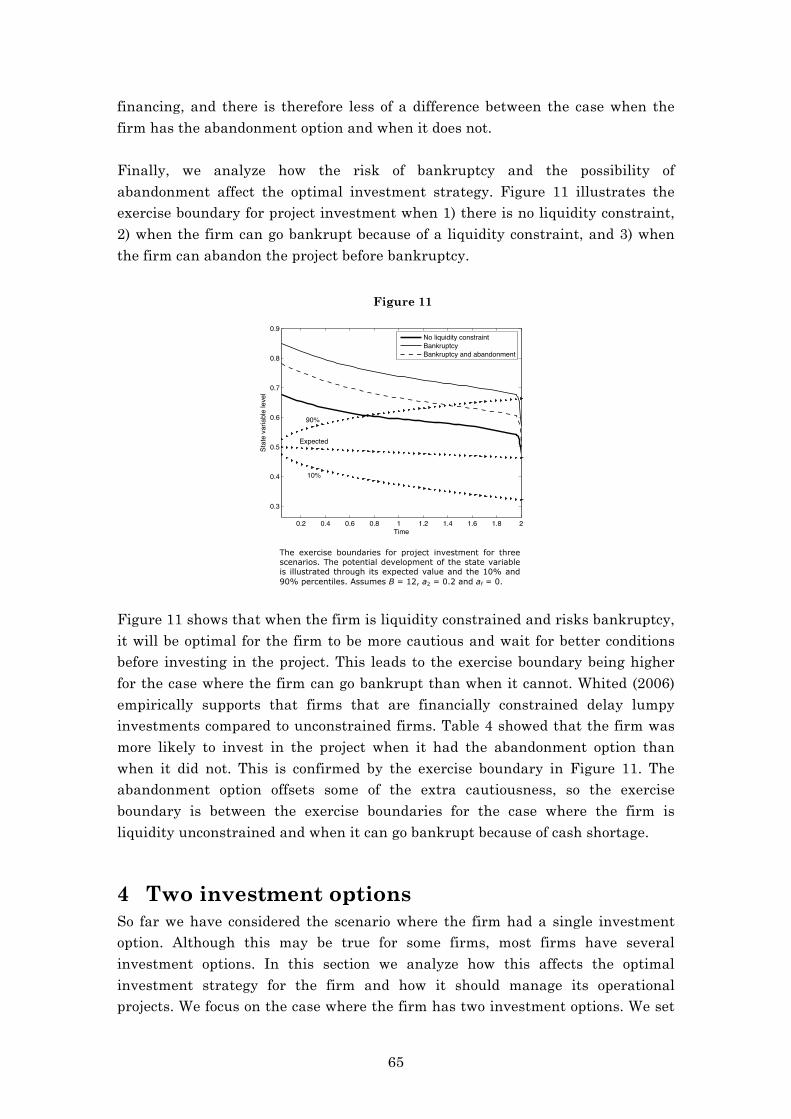
65

financing, and there is therefore less of a difference between the case when the firm has the abandonment option and when it does not. Finally, we analyze how the risk of bankruptcy and the possibility of abandonment affect the optimal investment strategy. Figure 11 illustrates the exercise boundary for project investment when 1) there is no liquidity constraint, 2) when the firm can go bankrupt because of a liquidity constraint, and 3) when the firm can abandon the project before bankruptcy.

Figure 11

The exercise boundaries for project investment for three scenarios. The potential development of the state variable is illustrated through its expected value and the 10% and 90% percentiles. Assumes B = 12, a2 = 0.2 and af = 0.

Figure 11 shows that when the firm is liquidity constrained and risks bankruptcy, it will be optimal for the firm to be more cautious and wait for better conditions before investing in the project. This leads to the exercise boundary being higher for the case where the firm can go bankrupt than when it cannot. Whited (2006) empirically supports that firms that are financially constrained delay lumpy investments compared to unconstrained firms. Table 4 showed that the firm was more likely to invest in the project when it had the abandonment option than when it did not. This is confirmed by the exercise boundary in Figure 11. The abandonment option offsets some of the extra cautiousness, so the exercise boundary is between the exercise boundaries for the case where the firm is liquidity unconstrained and when it can go bankrupt because of cash shortage. 4 Two investment options So far we have considered the scenario where the firm had a single investment option. Although this may be true for some firms, most firms have several investment options. In this section we analyze how this affects the optimal investment strategy for the firm and how it should manage its operational projects. We focus on the case where the firm has two investment options. We set

0.2 0.4 0.6 0.8 1 1.2 1.4 1.6 1.8 2

0.3

0.4

0.5

0.6

0.7

0.8

0.9

Time

Stat

e va

riabl

e le

vel

No liquidity constraintBankruptcyBankruptcy and abandonment

90%

Expected

10%

66

up the model, and review some of the extra considerations the firm must take into account when it has more than one investment option. We find that the inclusion of another investment option affects the value of the initial investment option, but that the effect depends on the cash flow profile of the new investment option. We also consider how bankruptcy and the abandonment option affect and is affected by the inclusion of another investment option. We see that in some instances a firm will be more likely to abandon a project, especially if the purpose is to protect another valuable project from bankruptcy.

4.1 Model framework

Assume the firm has the possibility to invest in two different projects, which are denoted h = {1 , 2} for Project 1 and Project 2 respectively. We assume the two investment options are available from the outset and that they are independent of each other in the sense that the firm can exercise the investment options in whichever order it chooses. However, the inclusion of another investment option affects the other investment option because of the impact it can have on the amount of liquidity available. When the firm has a single investment option, it decides when to invest in the project and whether to abandon the project once it is operational. The abandonment decision is made solely based on the impact it has on the individual project. However, when the firm has two investment options we cannot treat the two investment options independently in the same way. The cash flows from one project will affect the firm’s liquidity and risk of bankruptcy, which therefore also affects the other project. The total cash flows are given as specified by cft ! cfft ! cfot1 ! cfot2!,! (21)

where cfft is specified in (3) and cfoth for each of the projects is given by (20). This means that it might be optimal to abandon a project to subsidize the other, even though a stand alone analysis of the project would not lead to abandonment. The optimal decision rule for abandonment must take this into account. The firm value must also be modified, so that it reflects the value generated by both projects. The firm value is therefore calculated as specified by

FVt ! !! ! ! r ! s!t · cfos1 ! cfos2T

s=t

! CCt!!t ! B ! cfft !.! (22)

Compared to (7) and (8) in Section 2.1, we cannot set the present value of the future cash flows equal to the value of the individual options, and maximize firm value by using the optimal policy for the individual options. The projects are

67

interdependent because of the liquidity constraint, and the optimal policy must account for this. The maximization problem is given according to

maxts1!!!ta1!!!ts2!!!ta2!

FVt !,! (23)

as the firm must now make investment and abandonment decisions for both projects. The firm’s decision set grows more complex by including another investment option. The decision tree for the problem is depicted in Figure 12.

68

Figure 12

Illustration of the decision tree for the problem with two investment options on projects, which each have an abandonment option.

The decision tree is composed of 4 different types of nodes; invest, abandon, go bankrupt or wait. If the firm has not already invested in both projects it can choose to invest in one of the projects. Once the firm has an operational project it can choose to abandon it. Bankruptcy is an automatic process that happens once the amount of total cash is about to become negative. If the firm chooses not to exercise any of the options and it is not forced into bankruptcy, it waits. The firm

Wait

Invest in project 2

mirrors “Invest in project 1” node

Invest in project 1

Invest in project 2

Go bankrupt

Abandon project 1

Wait

Go bankrupt

Wait

Abandon project 2

Abandon project 1

Wait

Abandon project 2

Go bankrupt

Wait

Abandon project 1

Go bankrupt

Wait

Abandon project 2

Go bankrupt

Invest in project 2

Wait

69

will then be faced with the same possible decisions in the following period. Since bankruptcy is an automatic process and waiting is simply the opposite of choosing to invest or abandon, we need to find the optimal decision rules for when to invest in the project and when to abandon it. The optimal decision for when to invest in the project will be dependent on what we expect from the project once it is operational, which will be dependent on the decision rule for the abandonment option. We therefore start by analyzing the abandonment option, before analyzing the decision rule for the investment option.

4.2 Decision rules

A project can only be abandoned if it is operational and the decision is dependent on the state of the other project. We distinguish between three sets of decision rules, depending on whether the other project is: still an investment option, operational or abandoned. These also represent different stages in the decision tree as illustrated in Figure 12. Since the former abandonment decisions are dependent on the possibility of the future decisions, we need to calculate them in a specific sequence. We analyze each of them respectively below.

4.2.1 Last operational project

First, we analyze the case where there is only one operational project because the other project has been abandoned. We make a small addition to the notation to indicate the state of the two projects, since the value functions depends on the state of the other project. We therefore use o&a in Vt,p(h)

o&a,h to indicate the state of the project and the other project respectively, where o is used to indicate that the project is operational and a is used to indicate that the other project has been abandoned or has reached project maturity. When the other project has been abandoned, the firm only needs to consider whether it makes sense to abandon the project based on a stand-alone analysis. This is done by treating the abandonment decision as we did in Section 3.1 when we analyzed the problem for a single project. The optimal abandonment time is given as specified by

!tah ! !"# t ! tsh+!t,…,tsh+TP !! ! !!Vt,p(h)o&a,h xt

h!CCt ! Atsh,th xt

h !.! (24)

But note that compared to Section 3.1, we now have that the amount of cumulative cash CCt has been affected by the cash flows from both projects as specified by (21).

4.2.2 Both projects are operational

Next, we analyze the decision rule for the case in which both projects are operational. Here, the firm can choose to abandon one of the projects if it finds it

70

optimal to do so. In this case we cannot simply analyze the problem as an independent project because the expected cash flows from the other project will also affect the decision of whether or not to abandon the project. The abandonment value will be the same, since this is based on the value of the project without any constraints. The expected value from keeping the project operational, however, will be different. We denote this value Vt,p(h)

o&o,h, which is dependent on the variables of the other project. We use j to denote the project which is not project h, and let it be specified by

j ! !2 if h ! 1!1 if h ! 2 . (25)

First, we calculate which of the two projects leads to the highest total value upon abandonment. We denote this project ht

!, and let it be specified by

ht! ! arg!max

hVt,p(j)o&a,j xt

j, xth, ts

h, CCt ! Atsh,th xt

h ! Atsh,th xt

h !. (26)

Note, the total abandonment value accounts for the value which is added to the project that is kept operational because of the added liquidity acquired from abandoning the project. It is only optimal to abandon a project if the value of abandoning the project is higher than the value of keeping both projects operational. This leads to the abandonment time specified by:

!taht!! !"# t ! ts

ht!+!t,…,tsht

!+TP ! ! !!VOOt ! VOAt,p(ht!)

ht!

!where

VOOt ! !Vt,p(h)o&o,h xth, xt

j, tsj , CCt ! Vt,p(j)

o&o,j xtj, xt

h, tsh, CCt !

VOAt,p(ht!)ht!

! !Vt,p(j)o&a,j xt

j, xtht!, tsht!, CCt ! A

tsht!,t

ht!

xtht!

! Atsht!,t

ht!

xtht!!!

(27)

Note, the firm may choose never to abandon any of the projects.

4.2.3 One operational project and one investment option

Before both projects are operational, we have that one project is operational while the other project is still an investment option. In this case the firm can either decide to do nothing, exercise the remaining investment option or abandon the operational project. The firm may choose to abandon the operational project either because of the risk of bankruptcy or to raise the necessary liquidity to invest in the other project. Should it choose to invest in the other project it must also consider how the reduced available liquidity (from paying the investment cost) affects the value of the two projects. Let set # specify the values for each possible action, and let it be specified by

71

! !

Vt,p(h)o&i,h xt

h! xtj ! tsj !CCt ! FtC,j xtj ! xth! tsh!CCt ! !Vt,p(h)o&o,h xt

h! xtj ! tsj !CCt ! I ! FtE,j xtj ! xth! tsh!CCt ! !

Atsh,th xt

h ! FtC,j xtj ! xth! tsh!CCt ! Atsh,th xt

h

!. (28)

We assume the investment costs I for the two projects are the same. F denotes the value of the investment option. However, compared to Section 2.1 it is now also dependent on the state of the other project. Based on this set, the optimal action is specified according to:

Optimal action ! !wait if Vt,p(h)

o&i,h ! FtC,j ! !"#!!!invest!!!!ts! ! ! if Vt,p(h)

o&o,h ! FtE,j!!"!"#!!!abandon! tah ! ! if Atsh,t

h ! FtC,j!"!"#!!!!! (29)

These decisions are made every period and can change as the underlying state variable and the amount of cumulative cash change over time.

4.2.4 Only investment options

Based on the above decision rules it is possible to calculate the value of the project once it is operational. Based on this it is possible to make the necessary calculations for the investment options. This leads us to the decision of when to invest in the first project. First, we calculate which of the investment options has the highest value if exercised. Let ht

!! denote this project, which is specified by

ht!! ! arg!max

hFtE,h xt

h! xtj !CCt ! FtC,j xtj ! xth!CCt ! I !. (30)

Notice that the total investment value is dependent on the loss of value related to the remaining investment option caused by the reduction in liquidity by the investment cost. The firm only chooses to invest in the project if the value from investing in the project is higher than the value of keeping both investment options. The investment time for the first project is specified by

!tsht!!! !"# t ! 0,!t,…,TI ! ! !!FCCt ! FECtht

!!!

where

FCCt ! !FtC,h xth, xt

j, CCt +!FtC,j xtj, xth, CCt !

FECtht!!! !FtE,ht

!!xtht!!

, xtj, CCt +!FtC,j xtj, xtht

!!, CCt ! I .

(31)

72

Once the firm chooses to invest in the first project, we use (29) to determine the next optimal course of action. This ends the description of the decision rules.


Extending the model to two projects causes a significant extension to the numerical method. When the abandonment option for a single project was introduced, we extended the numerical method by first calculating the decision rule for the abandonment option. Only once this was done, was it possible to calculate the decision rule of whether or not to invest. The same principle applies when we have two investment options. First, we calculate the decision rules for each of the projects, when we assume the other project has been abandoned. This is very similar to the calculation of the abandonment and investment decision rules in Section 3.2, where the firm only had one investment option. The difference is that the firm’s liquidity now has been affected by the operations of the other project. We therefore include the amount of cumulative cash in the basis functions for the investment option, and vary the amount of cumulative cash to represent the other project. Once this is calculated, we calculate the abandonment decision rules for when both projects are operational. This uses the decision rules calculated for when one project is operational and the other is abandoned. Once this is calculated, we can use these decision rules to calculate the decision rules for when one project is operational and the other is still an investment option. Finally, we can use all these decision rules to calculate the decision rules for when both projects are still investment options. Based on these decision rules, it is possible to calculate the value of the firm.

4.4 Results

Section 2.4 showed that the cash flow profile is an important determinant for the value of the investment option when the firm has a single project. In this section we see how this also applies when the firm has more than one project. First, we analyze the effects that arise when the firm has two projects and no abandonment options. Once these effects have been firmly established, we consider the effects that arise because of the abandonment option. Where applicable, we assume the firm now acquires B = 14 in initial equity financing.

4.4.1 Prior operational projects

So far we have assumed the firm had made no prior investments before deciding to exercise its investment option. As a consequence, there were no operating cash flows generated until the investment was made. Lamont (1997) finds empirical evidence that some firms are highly dependent on cash flows from operational projects in one segment (e.g. the oil industry) to finance investments in other segments. We now analyze how the results in our model change, when we assume

73

the firm has a project which is operational from the outset. The operational project generates cash flows which affect the amount of liquidity available. How this affects the investment option depends on the investment option and the cash flow profile of the operational project. We assume the project related to the investment option is a growth project, and analyze how the type of the initial operational project affects the value of the investment option. Figure 13 compares the value of the investment option across different levels of initial liquidity when the firm has a prior project which is a cash cow, a prior project which is a growth project and when it has no prior projects.

Figure 13

Value of growth project investment option, when the firm already has an operational project that is either a growth project or a cash cow. The project cannot be abandoned.

For high amounts of external financing, the investment option is not affected by the prior operational project. However, for low amounts of external financing the investment option is affected by the cash flow profile of the prior operational project as it affects the amount of liquidity available to the firm. This is consistent with Faulkender and Wang (2006), who empirically examine the marginal value of liquidity for constrained firms. They find that the marginal value of liquidity is higher for firms with lower liquidity, greater investment opportunities, and higher external financing constraints. For low amounts of external financing, the operational project adds value no matter whether it is a cash cow or a growth project. Since the investment option is a growth project, there is a high likelihood that the firm will go bankrupt in the initial phase of negative cash flows unless more liquidity is added. A prior operational project causes variance in the amount of liquidity available. This adds value to the investment option, because the variance in the liquidity means that there is a probability that the firm will get enough liquidity to be able to exercise the investment option without the imminent risk of bankruptcy. The investment option has the most value when the prior operational project is a cash cow, since this increases the probability that the firm can invest in the new project.

10 11 12 13 14 15 16 17 18 19 200.5

1

1.5

2

2.5

3

3.5

4

4.5

5


Opt

ion

valu

e

No prior projectGrowth projectCash cow project

74

When the firm has intermediate amounts of external financing, the investment option eventually benefits from not having a prior growth project. There are two reasons for this. First, for these intermediate amounts of external financing, we have that the effect of the liquidity variance changes from being positive to negative. This is because the liquidity variance means that the firm may find itself in situations in which it would be optimal to invest in the project, but where it is impossible because of negative cash flows from the operational project. The investment option only needs the bare minimum of liquidity to ensure that it does not go bankrupt. It does not need any extra liquidity beyond that, and variance in the amount of liquidity therefore risks jeopardizing perfectly good exercise opportunities. Second, the prior operational project leads the firm to become more cautious regarding the investment option, because bankruptcy would now not only risk the cash flows of the project from the investment option, but also the cash flows from the prior operational project. Figure 13 illustrates that the firm does not have these concerns when the prior operational project is a cash cow, because the cash cow project generates positive cash flows from the beginning, which minimizes the risk of bankruptcy.

4.4.2 Multiple investments options

Next, we analyze the dynamics when the firm has two investment options, i.e. when the other project is no longer a prior operational project but instead an investment option as well. This means that the firm will have to pay the investment cost if it wants to make the other project operational (which we assumed had already been paid in the previous section), but that it can choose when and whether to invest in the other project. Like in the previous subsection we assume that the initial investment option is a growth project while the other investment option can be either a growth project or a cash cow project. In both cases, we find that the inclusion of another investment option affects the value of the option compared to if we had valued the option independently. But note that the inclusion of another investment option will always increase the firm value, because the value of the real options will always be non-negative. Figure 14 illustrates how the net firm value is dependent on the amount of equity financing. This is done for three cases: when the portfolio consists of just a single growth project, when the portfolio consists of two growth projects, and when the portfolio consists of a growth project and a cash cow project. From the figure we can see that the addition of another investment option always adds value, whether it be a growth project or a cash cow project. The firm can always choose never to invest in the project if it is not optimal. It is the cash cow project which adds the most value. There are two reasons for this. The first is that the cash cow project has a higher value when valued independently, because there is less of a risk that the project will go bankrupt because of cash shortage. This was

75

illustrated in Figure 8 and Figure 9. The second reason is that it is more likely that the cash cow project will earn back the necessary cash in time for the firm to be able to also invest in the growth project. In all cases we find that more initial liquidity increases the value of the portfolio. Note, that in the case with two growth projects, we see a relatively sharp increase in value when the amount of equity financing reaches 20. At this level of liquidity it is becomes more likely that the firm can invest in both projects, and it is therefore sensitive to increases in the amount of liquidity available.

Figure 14

Figure 15

Net firm value, FV0-B, for different amounts of external financing, for growth project investment option and different secondary investment option project types.

Value of investment option on growth project for different amounts of external financing, for different secondary investment option project types.

Figure 15 illustrates how the inclusion of another investment option affects the value of the initial growth project investment option. The value of the single investment option is the same as in Figure 8. Compare the value of the growth project investment option when it is the only investment option and when the firm has an additional growth project it can invest in. We see that the value of the initial investment option is reduced when including the additional investment option. For low amounts of external financing, the firm is constrained and it must make a choice between which of the projects to invest in. In some instances, it will be optimal to invest in the other investment option instead of the initial one. This reduces the value of the initial investment option. In some instances the project may generate enough cash so that the firm can invest in the second project as well. However, this is not very likely when both projects are growth projects. This is more likely when the other project is a cash cow project. From Figure 15, we see that this adds value. For low amounts of external financing we have that the value of the growth project is substantially increased when the firm has a cash cow project. This is caused by the same effect we had in Figure 13, so the firm can use the cash flows from the cash cow project to fund the growth project, which would otherwise most likely default.

10 15 20 250

1

2

3

4

5

6

7

8

9

10


Net

firm

val

ue

Single optionGrowth projectCash cow project

10 15 20 250

0.5

1

1.5

2

2.5

3

3.5

4

4.5

5


Opt

ion

valu

e

Single optionGrowth projectCash cow project

76

For intermediate amounts of external financing, Figure 15 shows that the value of the single investment option is slightly higher than when the firm can also invest in the cash cow project. This is because the firm is still constrained, so it may come in situations where it will have to choose between investing in one of the projects, and where the cash cow project will not be able to earn back the necessary liquidity in time for the firm to also invest in the growth project. Thus, although adding investment options to the portfolio does add value, it does not necessarily add the entire independent value of the investment option, because it may not be able to exercise the investment option because of lack of liquidity. The firm must keep this in mind when allocating resources to acquire new investment options. Not only is the value of the option itself reduced, it may also reduce the value of the other investment options in the firm’s portfolio. The negative effect on the initial option magnifies with the desirability of the other project, as it will be optimal for the firm to choose the other investment option instead of the initial option. However, an increased desirability of the other project will usually be connected with increased cash flows. If these are high enough so that it may fund the other project, it may only have a minor effect on the value of the less desirable investment option, as we can see in our case. The difference in the values in the three cases decrease when the firm less liquidity constrained, and are the same in the limit.

4.4.3 The value of the abandonment option

Next we consider how the inclusion of an abandonment option affects the problem with two investment options. In Section 3.3 we saw that the value of the investment option increases when the project has an abandonment option. This was measured by calculating the expected value of the project’s cash flows. However, when the firm has multiple options, management must be careful not to use this measure if it is considering selling some of the investment options. This is because the abandonment option may help increase the cash flows of other projects, and not just its own. Management should therefore not think that the project is worse because it has an abandon option, simply because the expected value of the project cash flows may be reduced. Table 5 illustrates the problem. We consider a firm which has two investment options. The two investment options are identical, except that investment option 1 has an abandonment option while investment option 2 does not. To capture the relevant effects, we assume the abandonment option gives the firm the option to resell the project, but not shut it down, so a1 = !. Based on this we calculate the individual value of the two investment options based on their cash flows. This is done for different levels of discount the firm needs to give in connection with selling the project. We start by observing that the total value of the two options increases as the abandonment costs decreases. This is expected, since having more options always adds value,

77

and decreasing the abandonment cost increases the probability that the abandonment option can be used.

Table 5 The effect of the option to abandon in a portfolio of options

a2 = 0% a2 = 20% a2 = 100%

Investment option 1 (has abandonment option)

4.32 3.40 3.77

Investment option 2 4.15 4.29 3.77

Total 8.47 7.69 7.54

Results show the value of each of the two investment options, based on the present value for that specific project. a1 = ! and a3 = 0. Assumes B = 14.

We see that the two investment options have the same value when the firm must give a discount of a2 = 100%. At this point, it will effectively never be optimal to resell the project, so the abandonment option is never used. When the firm can sell the project at its full value, for a2 = 0%, we see that the investment option with the abandonment option has the highest value. Having an abandonment option will increase the value of the specific project, because it can be sold and retain some of its value instead of being lost in bankruptcy. However, as we can see for a2 = 20%, this is not necessarily true for all specifications of the abandonment option. In this case we see that it is the investment option without the abandonment option that has the highest value. The reason we see these results is because there are two reasons to abandon the project. These two reasons have opposing effects on the individual investment option, but will always increase the total value of the options. It increases the value of the investment option, that the firm can receive a salvage value for the project and avoid losing all the value in bankruptcy. This was the effect the dominated for a2 = 0%. However, it may also be optimal to sell the project to finance the other project. This could be optimal, even though it would not be optimal based on a stand alone analysis of the abandonment option. This reduces the cash flows of the project to the benefit of the other project. This effect dominates for a2 = 20%. We give the abandonment decision a more careful analysis in the next section.

4.4.4 The abandonment decision

Having concluded that the abandonment option affects the value of both options in the portfolio, we turn to give a more careful analysis of how the abandonment decision changes with the inclusion of another investment option. With a single project, the firm will either shut down the project when the value of the project is less than the abandonment cost, or resell it when the salvage value is higher than the project value (given the financial constraint). This occurs for low to intermediate market conditions, where the project has a positive value, but where

78

there is a high probability that the firm will go bankrupt because of cash shortage. The abandonment decision is illustrated in Figure 16.

Figure 16

Figure 17

Illustration of abandonment decision for single growth option. Illustration for project started at ts

h = 0.5 at t = 1.5. Parameters: a1 = 0, a2 = 0.2, a3 = 0, B = 14, CCt = -13.3.

Comparison of the abandonment boundary for a single project and where there is another investment option. The projects are identical growth projects as the ones depicted in Figure 16.

We now consider the scenario when the firm has an additional investment option besides the initial project it has invested in. The abandonment decision will no longer be based only on the variables related to the project itself, but also on the state variable of the other investment option. Figure 17 compares the abandonment boundary for the case where the firm has a single project to the case where it has a project and a second investment option. It illustrates at what level of state variable 1 (the market conditions for the project the firm has already invested in) the firm should abandon the project given the level of state variable 2. When the firm only has the single project we see that the abandonment boundary will be independent of the other project and it will equal the abandonment boundary found in Figure 16 for all values of state variable 2. Now turn to the case where the firm has another investment option besides the operational project. The abandonment boundary for the operational project will be the same as in the single project scenario when the market conditions for the second investment option are bad. Since the project values in this case will be low or negative, there is a low probability that it will ever be exercised, so this should not affect the abandonment decision of the operational project. However, improving market conditions for the second investment option leads to the second investment option having an effect on the abandonment boundary of the operational project. First, we see that the initial abandon boundary decreases, so the firm will be inclined to keep the project in worse market conditions before it chooses to abandon the project. This result is based on the premise that the firm

0.25 0.3 0.35 0.4 0.45 0.5 0.55 0.6 0.65 0.7 0.750

5

10

15

20

25

30

Statevar 1

Valu

e

Project valueSalvage value

0.25 0.3 0.35 0.4 0.45 0.5 0.55 0.6 0.65 0.7 0.750.25

0.3

0.35

0.4

0.45

0.5

0.55

0.6

0.65

Statevar 2St

atev

ar 1

Single optionPortfolio of options

Abandon if portfolio of options

Abandon if single option Abandon if portfolio

of options

79

does not already have enough liquidity to invest in the second investment option. This gives the firm an incentive to keep the project, as there is a probability that it will generate enough cash to be able to invest in the other project. If it abandons the project, it will never have enough liquidity to make the investment, and it will in effect forfeit the investment option. The better the market conditions for the second investment option, the more the firm has an incentive to keep the initial project, even though it is suboptimal based on a stand alone analysis. Second, as the market conditions for the second investment option improve, we see that an upper abandon boundary emerges. At these market conditions for the operational project, the firm can resell the project at a price that is high enough so it can invest in the second project. If the market conditions are very good, it may still be optimal to keep the project however, as the percentage discount given when selling the project would more than offset the value gained from being able to invest in the second option. This leads to the steep upward sloping boundary, such that higher values of state variable 1 requires a higher value of state variable 2. Note, that according to the upper abandonment boundary it is optimal to abandon the project when the market conditions for Project 2 are better than the market conditions for Project 1. This depends on the amount of time left to maturity for the investment option. If there is enough time left to maturity, there is a probability that Project 1 will be able to generate all of the necessary liquidity without being abandoned. If there is a short time left to maturity, we find the opposite result, so the firm will abandon the project for values of state variable 2 that a lower than state variable 1. At this point, the firm prefers to ensure that it has the necessary liquidity to be able to invest in the second investment option, and it is therefore more inclined to invest. 5 Conclusion The paper has presented a model where liquidity concerns affects the investment and abandonment of projects. We found that liquidity constrained firms prefer cash cows to growth projects, since cash cows reduce the risk of bankruptcy because of cash shortage. We found that the risk of bankruptcy makes the firm less likely to invest in the project when the amount of liquidity is reduced. We found that the abandonment option adds more value as the amount of external financing is reduced. Instead of losing the entire project value through bankruptcy, the abandonment option gives the firm the option to sell of the project so it can retain some of the project value. This affects the probability of bankruptcy and the firm’s optimal investment policy. The abandonment option helps mitigate some of the bankruptcy risk that makes the firm more cautious, so that it will invest at lower thresholds.

80

When the firm has multiple projects, we find that the cash flows from one project can be used to finance the other project. This means that the cash flow profile of the project is important to other projects than simply the project itself. We also find that the inclusion of other projects may make the firm more cautious in investing in new projects, because it does not want to risk losing the projects to bankruptcy because of overinvestment. Finally, we found that the abandonment option may be used not only to the benefit of the project it is attached to, but also to other projects at the firm’s disposal. This means that the firm may choose to sell a project to acquire the necessary funds to invest in another project.

81

References Almeida, Heitor; Campello, Murillo and Weisbach, Michael S., 2011, “Corporate Financial And Investment Policies When Future Financing Is Not Frictionless”, Journal of Corporate Finance, Vol. 17, pp. 675-693 Boyle, Glenn W. & Guthrie, Graeme A., 2003, “Investment, Uncertainty, And Liquidity”, Journal of Finance, Vol. 58, No. 5, pp. 2143-2166 Brennan, Michael J. and Schwartz, Eduardo S., 1984, “Optimal Financial Policy And Firm Valuation”, Journal of Finance, Vol. 39, No. 3, pp. 593-607 Bris, Arturo; Welch, Ivo, and Zhu, Ning, 2006, “The Costs of Bankruptcy; Chapter 7 Liquidation versus Chapter 11 Reorganization”, Journal of Finance, Vol. 61, No. 3, pp. 1253-1303 Brosch, Rainer, 2008, “Portfolio Of Real Options”, Lecture Notes in Economics and Mathematical Systems, Springer Bryan, Daniel M.; Tiras, Samuel L. and Wheatley, Clark M., 2002, “The Interaction Of Solvency With Liquidity And Its Association With Bankruptcy Emergence”, Journal of Business Finance & Accounting, Vol. 29, Issue 7-8, pp. 935-965 Dixit, Avinash K. & Robert S. Pindyck, 1994, “Investment Under Uncertainty”, Princeton University Press, Princeton Faulkender, Michael and Wang, Rong, 2006, "Corporate Financial Policy And The Value Of Cash", Journal of Finance, Vol. 61, No. 4, pp. 1957-1989 Gamba A., 2003, “Real Options: A Monte Carlo Approach”, Handbooks in Finance: Real Options by G.A. Sick and S. Myers (eds.), North Holland, accepted for publication. Hennessy, Christopher A. & Whited, Toni M., “How Costly Is External Financing? Evidence From A Structural Estimation”, Journal of Finance, Vol. 62, No. 4, pp. 1705-1745 Hirth, Stefan & Viswanatha, Marc, 2011, "Financing Constraints, Cash-Flow Risk, And Corporate Investment", Journal of Corporate Finance, Vol. 17, pp. 1496–1509

82

Lamont, Owen, 1997, “Cash Flow And Investment: Evidence From Internal Capital Markets”, Journal of Finance, Vol. 52, No. 1, pp. 83-109 Leland, Hayne, 1994, "Corporate Debt Value, Bond Covenants, And Optimal Capital Structure", Journal of Finance, Vol. 49, No. 4, pp. 1213-1252 Longstaff, Francis A. & Schwartz, Eduardo S., 2001, “”Valuing American Options By Simulation: A Simple Least-Squares Approach”, The Review of Financial Studies, Vol. 14, No. 1, pp. 113-147 Lyandres, Evgeny, 2007, “Costly External Financing, Investment Timing, And Investment-Cash Flow Sensitivity”, Journal of Corporate Finance, Vol. 13, pp. 959–980. Meier, Helga; Christofides, Nicos & Salkin, Gerry, 2001, “Capital Budgeting Under Uncertainty”, Operations Research, Vol. 49, No. 2, pp. 196-206 Miao, Jianjun and Wang, Neng, 2011, “Risk, Uncertainty, And Option Exercise”, Journal of Economic Dynamics & Control, Vol. 35, pp. 442-461 Pratap, Sangeeta and Rendon, Silvio, 2003, "Firm Investment In Imperfect Capital Markets: A Structural Estimation", Review of Economic Dynamics, Vol. 6, pp. 513-545 Whited, Toni M., 2006, “External Finance Constraints And The Intertemporal Pattern Of Intermittent Investment”, Journal of Financial Economics, Vol. 81, pp. 467–502

83

Appendix A This appendix gives an estimate of how precise the LSM method is given the parameters chosen for the numerical method. We compare the estimates of the basic problem (a single investment option with no abandonment option and no financial constraints) for the LSM method to the estimates that can be found using other numerical methods. We have not found any papers that analyze comparable results under the assumption that the firm can go bankrupt because of the liquidity constraint, after it has invested in the project. The LSM method is used to calculate the 1) present value of the project and 2) the value of the investment option. To compare the results of calculating the value of the investment option with other numerical methods, we must first calculate the present value of the project. To do this, we assume that the project does not have a cash flow profile, so "

h = 0. We set s0

h = 0.965 so that the present value of the project when investing at time t = 0 is equal to 1.8, cf. Section 2.3. To calculate the net present value of the project, we calculate the present value of the contribution margin and fixed costs separately. We calculate the present value of the contribution margin using chapter 6 in Dixit & Pindyck (1994),

!PV contribution margin ! !!hs0h1 ! exp ! r ! µ TP

r ! µ ! 41.98!!!

We calculate the present value of the fixed costs as the present value of an annuity,

!PV fixed costs ! fc1 ! 1 ! r !TP

log(1 ! r) ! 30.18!.!

We assume the investment cost is I = 10, as specified in Section 2.3. The net present value therefore becomes !NPV project ! PV contribution margin ! PV fixed costs ! I ! 1!8!.!

Using the same calculations, we can calculate the net present value for different values of xth. Based on these calculations of the present value of investing in the project, we can calculate the value of the investment option using the binomial tree and finite difference method. The value estimates for the different numerical methods can be seen in Table 6.

84

Table 6 Estimation of investment option value

Numerical method

Investment option

Project value at t = 0

LSM 4.6414 1.7653 Binomial tree 4.6644 1.8013 Finite difference 4.6634 1.8013

Estimation of the value of the investment option and project value when the firm is financially unconstrained. The estimates for the LSM method are the average of 100 estimations, with 200.000 simulations. For the 100 estimations, we find a min value estimation of 4.5908 and a max estimation value of 4.7024. For the binomial tree, we use 1024 time steps. For the finite difference method, we use 200 time steps and 1000 asset steps.

From the table we can see that the estimates are relatively close to each other. We make 100 estimations using the LSM-method, and find the smallest estimation value to be 4.5908 and the biggest estimation value to be 4.7024. Based on these calculations, we conclude that the LSM method with the chosen parameters is precise enough for the purposes of this paper.

85

Appendix B !t Annual time increment h Designation of specific project TI Years before investment option matures I Investment cost TP Project lifetime cfot

h After tax operating cash flow t Current time T Total time horizon in problem xt! State variable µ Drift for state variable ! Standard deviation for state variable ts! Time the firm decides to invest in project

p Time the project has been operational fc Fixed cost s0h Start level for cash flow profile "h Factor with which cash flow profile increases / decreases B Amount of external funds from equity CCt Cumulative cash generated by projects cfft Cash flows from financial activities r Risk free rate tb Bankruptcy time FVt Firm value Fth Value of investment option FtE,h Exercise value of the investment option when investing in

the project FtC,h Continuation value of the investment option from not

investing in the project tah Abandonment time for project h Vt,ph Project value of project once it is operational Vt,ph!" Value of project, when it is financially unconstrained Atsh,th Project abandonment value

a1 Cost of shutting down the project a2 Discount percentage given when selling project a3 Constant transaction cost when selling project af Fixed transaction costs a1 and a3 Vt,p(h)o&a,h Value of project h, when project h is operational, and the

other project has been abandoned. j The project which is not project h ht! Project with highest value upon abandonment when bot

projects are operational Vt,p(h)o&o,h Value of project h, when both projects operational

86

# The values for each possible action, when one project is operational and the other project is an investment option

Vt,p(h)o&i,h Value of project h, when project h is operational, and the

other is an investment option. ht!! Project which leads to the highest value if exercised, when

both are still at an investment option stage.

LIQUIDITY AND THE OPTIMAL CAPITAL STRUCTURE



March 2014

Abstract This paper develops a model where capital structure decisions are centered around the firm’s liquidity needs, while still accounting for tax benefits, the cost of financial distress and collateral. Transaction costs, the expected timing and uncertainty of cash flows all affect the optimal amount and preferred maturity structure for debt. Opportunity costs make it optimal to minimize excess cash in the firm, but transaction costs to raise funds means that cash should not be paid out too early. We show that cash flow characteristics affect the optimal capital structure, and that the firm will choose more leverage when it is a cash cow. We show that the firm should choose a schedule for debt payments which matches the firm cash flows, to minimize excess cash. Finally, we show that the firm will prefer to use long term debt as base capital to minimize transaction costs, and short term debt to dynamically adjust the amount of leverage.

Keywords: JEL classification: C61, C63, D92, E22, G32, G33, G35

Martin Schultz-Nielsen, Department of Economics and Business, Building 2622, Aarhus University, DK-8000 Aarhus C, Denmark, +45 87 16 53 18, [email protected]. The author would like to thank Andrea Gamba, Claus Munk, Peter Ove Christensen, Jens Riis Andersen and the participants of the Aarhus University Finance Seminars for helpful comments.

*

Multiple real options, Liquidity constraints, Least-Squares Monte Carlo, Bankruptcy, Abandonment, Capital structure

90

1 Introduction Firms that incur external financing costs face a complex decision when they optimize the capital structure with respect to tax benefits, bankruptcy risk and financing costs. Financing costs means that the firm’s future liquidity needs must be accounted for when deciding on the optimal capital structure. The firm’s liquidity needs impact the optimal payments to equity holders and the optimal maturity structure and payment schedule for debt. By choosing a capital structure where funds are paid back faster than the firm can generate cash flows, the firm will be forced to acquire further external financing and pay transaction costs in the process. Firms will try to minimize these transaction costs, by optimizing the capital structure with respect to the project cash flows and the firm’s future liquidity needs. Bolton, Chen and Wang (2011) and Riddick and Whited (2009) analyzed the value of liquidity and the firm’s propensity to save. Their models are based on a dynamic trade-off between the opportunity cost of keeping cash and future financing costs. The results in our paper are based on the same trade-off. However, their analysis does not answer how the dynamic trade-off impacts the capital structure. The dynamic trade-off means that the firm’s cash flow profile, i.e. the expected timing and uncertainty of project cash flows, will have an impact on the optimal capital structure. The contribution of this paper is an analysis of how the optimal capital structure is affected by the firm’s cash flow profile and liquidity needs. The analysis requires that we develop a model where capital structure decisions are centered around the firm’s liquidity needs. We propose a novel way in which this can be done. We find that firms that have cash cow projects, which generate big positive cash flows from the beginning, will prefer to fund themselves with more debt than firms that have comparable growth projects. Because cash cow projects generate cash quickly, the firm can afford to pay bigger interest payments without having to seek further financing and pay transaction costs in the process. Firms will prefer debt types where the debt payment schedule can match the cash flows generated by the firm. If debt is paid back too slowly, it will lead to an excessive cash reserve being built up. This is costly because of the opportunity cost of keeping cash in the firm, as equity holders can generate a higher return by investing excess cash themselves. Firms can reduce the probability of an excessive cash reserve being built up by choosing an appropriate debt payments schedule or by choosing a short debt maturity so the amount of debt can be adjusted dynamically. Firms will therefore optimize both the amount, type and maturity of debt to their liquidity needs. The model also allows us to analyze how the capital structure is affected when the firm can issue both long term and short term debt. We find that the firm prefers long term debt over short term debt as base capital, because it reduces the transaction costs over the firm’s lifetime. Short term debt is used to dynamically

91

change the firm’s leverage over time, so the firm can flexibly increase its leverage in good conditions when additional debt financing is cheap. The paper can be related to several papers in the literature. The seminal paper by Leland (1994) examined how tax benefits from debt financing should be balanced with the cost of financial distress. This effect is also captured in our model. Leland (1994) assumes debt has an infinite maturity and that the face value of debt remains constant. Leland and Toft (1996) extended the model by letting debt have a finite maturity. However, the debt structure in the model is still stationary, so new debt is continuously issued with the same face value as the debt that is retired. Goldstein, Ju and Leland (2001) developed a model that allows for increases in the amount of debt over time. In our model, we allow the firm to choose the amount of debt it wishes to acquire when old debt matures, so that the amount of debt can both increase or decrease over time. Goldstein, Ju and Leland (2001) also note that the treatment of taxes as an inflow in the Leland (1994) model leads to the misleading result that increasing the tax rate increases the equity value (because of increased tax benefits). They solve this by using an EBIT-based model and treat taxes as reduced outflow. Our model is a cash flow based model and also treats taxes as a reduced outflow. Uhrig-Homburg (2005) extended the model by Leland (1994) by introducing transaction costs to the issuance of equity. The resulting model captures cash flow shortage as a reason to go bankrupt, even though the equity value is positive. In our model we also have transaction costs related to raising capital, which affects the preferred form of financing. However, in Uhrig-Homburg (2005) and Leland (1994) it is implicitly assumed that all excess cash is paid out to equity holders. In our paper we allow the firm to have excess cash, so dividends are an explicit choice. Riddick and Whited (2009) find that firms hold higher precautionary cash balances when external finance is costly or income uncertainty is high. Our model can be used to find similar results. All external financing takes the form of equity, so the paper does not analyze the effects it has on the capital structure as we do in our paper. Bolton, Chen and Wang (2011) develop a risk management model that unifies the optimal cash holding strategy with hedging possibilities. However, the paper also has a limited analysis of the capital structure. Both papers allow for continuous investment and disinvestment. We assume the firm invests in one investment and that no further investments are needed in the projects after the initial investment. Gamba and Triantis (2008) allow the firm to finance itself with debt and equity. They find that it may be optimal for the firm to borrow funds and still keep a cash reserve if external financing is costly. We can find similar results using the model presented in this paper. However, we do not assume that the interest rate is necessarily equal to the risk free rate, by assuming that debt is always covered by collateral. Instead, we explicitly model the value of the fixed assets that can be

92

used as collateral, so the interest rate on debt is dependent on the value of collateral and the firm’s financial outlook. Morellec (2001) finds that assets affect the firm’s optimal capital structure, e.g. that firms that have assets with a high liquidation value will prefer higher leverage ratios. The incorporation of fixed assets in our model allows us to find the same results. Hackbarth and Mauer (2012) analyze the effects of the debt priority structure when the firm has multiple debt issues. They find that firm conditions affect whether the firm prefers senior or junior debt. We find that the preferred type of debt is also dependent on the debt’s payment schedule and maturity. We analyze the effects of having long term and short term debt, where long term debt is senior. We find that the firm prefers long term debt if the debt payment schedule matches the firm’s cash flow profile, because it minimizes the expected transaction costs. We also find that it is not obvious whether giving the firm the option to finance itself with short term debt increases or decreases the value of equity, because it may lead long term debt holders to require a higher interest rate. These related papers assume the firm makes continuous real investments in the same market. This means it can operate indefinitely, and generate cash flows that follow the same stochastic process. In our paper, we assume the firm makes a lump sum investment and the resulting project has a finite horizon. This leads to some special dynamics. The model can be extended so that the firm can invest in more than one project, which can have different cash flow dynamics than the initial project. This would affect how the firm finances itself. We develop a model based on the following assumptions. We assume the firm has decided to invest in a project and now has to decide how to finance the investment. The investment costs are used on a combination of fixed assets and other expenses. The value of the fixed assets is stochastic and is sold at the end of the project, while the other expenses are assumed sunk. We find that the size of the fixed assets affect both the interest rate required by debt holders and the firm’s optimal financing strategy. This means that the firm’s asset composition, and not just average unlevered firm variance, matters in the firm’s financing. Upon defaulting on payments and when the firm is unable to acquire further funding, the firm defaults and is liquidated with bankruptcy costs. The size of the bankruptcy costs also affect the optimal financing of the firm. We assume that investors can get a higher return from investing excess funds themselves, rather than the letting the firm invest the money. This means that it is optimal to pay out unused cash reserves. The firm can finance itself with equity or debt. We illustrate how liquidity concerns affect the choice of financing. The remainder of the paper is organized as follows. Section 2 sets up the basic structure of the model, and illustrates the model in a deterministic setting.

93

Section 3 extends the model to a stochastic setting, and allows the firm to make financing decisions regarding both equity and debt. This model is used to show illustrative results. Section 4 makes another extension of the model, such that the firm can finance itself with both long term and short term debt. This is followed by another set of results. Section 5 concludes. 2 Initial Model This section set up the core dynamics of the model and illustrates the basic dynamics of the model in a simple setting. In this simple setting, we assume cash flows are deterministic and that the firm can only refinance itself using equity. In the following section, we allow cash flows and the value of fixed assets to be stochastic, and model the cash flows from financial activities. This extension will build on the core dynamics set up in this section.

2.1 Model

Our model is based on the following assumptions. The firm has a project which has a finite lifetime of T years. The project, and all of the assets related to the project, will at this point be liquidated. While the project is operational, it generates cash flows cfot. To keep the firm operational, the firm must always have a non-negative amount of liquidity or it will be forced into bankruptcy. To identify the firm’s liquidity needs, we introduce variables for the amount of liquidity at the firm’s disposal. The amount of liquidity in the firm is affected by the cash flows generated from operating the firm and the funds acquired from financing the firm. To distinguish value creation from financing, we keep the two sources of liquidity separate. The amount of liquidity from operating the firm is given by the cumulative cash flows CCt. The total amount of external financing is denoted by Bt. The firm can finance itself using equity, Bt

E, or debt, BtD, so the total amount of

external financing is specified by Bt = Bt

E + BtD!.! (1)

Note, that these amounts do not denote the value of debt or equity. They are simply a measure for how much liquidity has been injected into the firm from these sources of funding. They also make up the control variables in the model. The amount of equity Bt

E will change over time, if it is optimal for the equity owners to withdraw or inject more equity into the firm. The amount of debt may also change over time as the debt is paid back (or more debt is chosen). Interest on debt generate negative cash flows, which are captured by the cash flows from financial activities, cfft. Based on the operating and financial cash flows we calculate the total firm after-tax cash flows,

94

cft = cfot!+ cfft! ! ! tax , 0 ! t ! min (tb , T)

0 , min tb , T < t!,! (2)

where tax is the corporate tax rate and tb is the time the firm goes bankrupt (if it ever goes bankrupt). Based on these cash flows it is possible to calculate the cumulative cash CCt generated or required by the project as

CCt = cfs

t

s=0ds!.! (3)

Note that it can be negative. Bankruptcy occurs when the amount of external financing Bt is not enough to cover a deficit, i.e. when the total amount of cash in the firm is negative. Upon bankruptcy, the firm is liquidated and the assets are sold, so bankruptcy can only occur once. The time tb where bankruptcy occurs is therefore given by tb = inf t!!!!0 , T! : CCt + Bt < 0 !. ! (4) Note that the amount of external liquidity Bt is dynamic, so the firm can seek new financing before it goes bankrupt. However, the firm will only get additional funding if it is in the best interest of the equity holders. We elaborate more on these dynamics later in this section. In case of bankruptcy, the firm is liquidated, and the value is distributed to claimants. The value of the firm consists of three parts: 1) the amount of remaining liquidity, 2) the value of the firm’s operations and future profit potential and 3) the value of the fixed assets At. If the firm goes into bankruptcy, there can still be value in the firm’s future profit potential. However, the firm’s assets and future profit potential will usually be affected by bankruptcy, and the firm can therefore expect to get a lower value when it is sold in a fire-sale than if it kept it as a going concern. We capture this along with other bankruptcy costs through !. We assume claimants will simply shut down the firm if the resale value is negative, and that this can be done without any costs. When the firm reaches the end of the project at time T, it is also liquidated. However, in this case the firm does not suffer from a fire-sale loss, and the fixed assets are sold at their full value. The firm’s liquidation value is calculated by

!LVt = max( 0 , (CCt + B!!) +!(1-!)UVt + (1-!)At·(1-tax) ) , t = tb

max( 0 , (CCt + B!!) + At·(1-tax) ) , t = T!.! (5)

We use t! to specify the time right before the finance decision has been made. Since the firm’s liquidation value will be paid out to claimants, this will change the value at Bt. We assume the assets can be sold to a firm which is financially

95

unconstrained. UVt is the value of the firm’s future cash flow potential when it is financially unconstrained. Letting the risk free rate be denoted by r, and assuming all stakeholders are risk neutral, we calculate UVt as

UVt = !t exp (-r·(s-t))!cfos!!1!tax! dsT

s=!!!.! (6)

Upon liquidation, the liquidation value is distributed to claimants. We assume the absolute priority rule applies, so debt holders have seniority and must be compensated first, while equity holders get any of the remaining value. This means that the payments to each group of claimants are calculated according to

LVt

D ! min(LVt , B!!D ) ! t = min(tb!, T)

LVtE ! LVt - LVt

D ! t = min(tb!, T)!.! (7)

In (7), LVt

D is the payments to debt holders upon liquidation and LVtE is the

payments to equity holders upon liquidation. Before the firm is forced into bankruptcy, it can get additional financing. The firm will finance itself with the objective of maximizing the value to equity holders, cf. Uhrig-Homburg (2005) and Gamba and Triantis (2008). This means that financing decisions will be made irrespective of how it affects debt holders, management or other stakeholders. The amount of equity in the firm can change over time, as equity holders may inject more equity into the firm or pay out some of the firm’s liquidity as dividends. In the simplified setting in this section, we assume the amount of debt is exogenously specified, and the firm cannot make any decisions regarding debt. This is extended in the next section. Similar to related papers, we model the equity holders as a representative individual. This means that we do not consider issues related to how much firm share a new investor should get for injecting funds into the company, but simply focus on maximizing the total value to equity holders. Assume equity holders can choose equity amounts within the bounded interval specified by EQpos = emin!! emax !.! (8)

The value of the firm to equity holders is dependent on the amount of cash they expect to get from the firm, the amount of cash injected in the firm, and the equity holders required return on invested capital. The equity value is calculated as

96

EVt = !t !cfes ! exp -r·(s - t) !dsT

s=t

!,1! (9)

where the cash flows to equity holders mirrors the cash flows the firm acquires from equity financing cfet. We assume equity holders are risk neutral and that their required return is equal to r. To simplify notation, we assume that there are no personal taxes, cf. Riddick and Whited (2009). The equity value is dependent on how the firm finances itself today, and assumes that the firm will finance itself optimally in all future periods. The changes in equity, cfet, are decided by equity holders up until time T where the remaining value of the firm is paid out. The remaining value at this point is dependent on the choices that have been made up until time T. For debt holders to have an incentive to lend the firm money, they must be ensured that the firm will not funnel out funds to equity holders and leave the debt holders with nothing. To ensure this, we assume that the debt agreement includes covenants that details when equity holders can pay out funds. We assume that equity holders abide to these contractual agreements. Debt covenants can be designed in a lot of ways. See Gamba and Triantis (2013) for an analysis of the effectiveness of debt covenants. In this paper we assume that 1) the firm is not allowed to pay out funds to equity holders if it results in the firm liquidation value falling below the face value of debt and 2) the firm is not allowed to sell the firm’s fixed assets without immediately paying off debt holders, cf. (7). The debt covenants cannot force the equity holders to inject more equity capital than they have already injected, although they are free to do so if it is optimal. The equity holders also cannot pull out money which is not there, which means that the total amount of liquidity in the firm must be non-negative. Although it is a relatively simple contract, it will be sufficient with the examples we wish to illustrate in this paper. These conditions specify the subset EQsub of possible equity amounts that can be chosen. It is given by

EQsub = e ! EQpos | CCt+ e+BtD > 0 ! Bt

D < LVt(e) if e < Bt-E !.! (10)

Based on these possible equity amounts, the firm chooses the amount of equity funding B!

E! that maximizes the value to equity holders. This is specified later in this section. The firm continuously decides on the optimal amount of equity, until the firm either defaults or reaches maturity, at which point the remaining value in the firm is paid out. This is represented by

1 We include jumps by adding them separately

97

!cfet !B!E* ! Bt-E , 0 ! t < min(tb , T)

!LVtE , t = min(tb , T)0 , min(tb , T) < t

! !! (11)

where LVt

E is the liquidation value to equity holders defined in (7). Based on the conditions for financing described above, the firm decides on how to optimally finance itself. In the simplified setting in this section, we assume the amount of debt is exogenously specified. This means the firm can only make decisions regarding the amount of liquidity from equity holders. For each period, the firm chooses the amount of equity that maximizes the value to equity holders,

B!E! = arg max

eEVt e , Bt

D | e ! EQsub !.! (12)

The equity value includes the cash flow the equity holder injects/withdraws from the firm, to achieve the specified level of equity in the firm. It is these maximizations which determine whether it is optimal to let the firm default or keep the firm operational by injecting additional equity.

2.2 Example of firm refinancing

In this example, we illustrate the firm’s refinancing choice and the sequence of decisions in the model. Assume equity holders have inherited a firm. The firm was initially financed with equity, but these funds have all been lost while operating the firm. This means we currently have a situation where B0 !!B0E = 10 and CC0 = -10. The firm has a project with known discrete cash flows. These are given in Table 1.

Table 1 Cash flows and initial financing

t 0 1 2 3 4

cft -5 0 0 10 CCt -10 -15 -15 -15 -5 Bt = Bt

E 10

Although the firm has previously been unprofitable, the new equity holders have inherited a project which could make them a profit. At t = 1, the firm incurs a negative cash flow, and the equity holders have to decide whether it is optimal to inject additional equity into the firm or if it is better to let the firm go bankrupt. Assume the risk free rate is r = 5%, bankruptcy cost is ! = 0.25 and tax = 0.

98

If the equity holders do not inject additional equity, the firm goes bankrupt. Upon bankruptcy the firm sells its assets and distributes the liquidation value to the claimants. We use equations (5) – (7) to calculate the value of this choice to equity holders. First, we use (6) to calculate the value of the firm’s cash flow potential, UVt. The project will generate a positive cash flow at t = 4. The value of this can be calculated to UV1 = exp(-0.05·(4-1))·10 = 8.61!!!

This can be used to calculate the liquidation value using (5). Since there are no debt holders, this is also equal to the value to equity holders, so EV1 ! LV1 = max(!0 , (-15+10) !"0.75!8.61) = 1.46!.!

Equity holders therefore get a positive liquidation value from letting the firm default. We must compare this to the value equity holders would get if they injected equity into the firm and kept it from bankruptcy. The cash flows between the firm and equity holders for this scenario can be seen in Table 2.

Table 2 Cash flows and choice of financing

t 0 1 2 3 4

cft -5 0 0 10 CCt -10 -15 -15 -15 -5 Bt = Bt

E 10 15 15 15 5 cfet 5 0 0 -10

The value from these cash flows can be calculated using (9): EV1 = -5!!"exp(-0.05·(4-1))·10 = 3.61!.!

Since the value of injecting additional capital is higher than the liquidation value, it is optimal for equity holders to inject additional equity and keep the firm operational.

2.3 Example of firm default

Assume now that equity holders have inherited a firm that is identical to the firm in the previous example. However, this time the firm was initially financed with a bullet bond in addition to equity. This means we currently have a situation where !B0E = 5, B0

! = 5 and CC0 = -10. The coupon payments on debt leads to cash flows

99

from financial activities that equal cfft = -0.30. The cash flows and the initial financing can be seen in Table 3.

Table 3 Cash flows and initial financing

t 1 2 3 4

cfot -5 0 0 10 cfft -0.3 -0.3 -0.3 -0.3 cft -5.3 -0.3 -0.3 9.7 CCt -10 -15.3 -15.6 -15.9 -6.2 BtE 5 BtD 5

Bt 10

We assume the bullet bond matures and must be paid back at t = 4. The equity holders must again decide whether to inject additional equity and keep the firm from bankruptcy at t = 1. Again, we begin by calculating the value from bankruptcy. Since the underlying firm is identical, the value of the firm’s cash flow potential, UVt, will be the same, so using (6) we can again calculate UV1 = exp(-0.05·(4-1))·10 = 8.61!.!

The firm’s liquidation value, LVt, will be slightly lower because of interest payments at t = 1, LV1 = max(!0 , (-15.3+10) !"(1!!)!8.61) = 1.16!.!

This time debt holders must get their share of the liquidation value. We use (7) to calculate the value to equity holders,

LV1

D ! min(1.16 , 5) ! 1.16

LV1E ! 1.16 - 1.16 ! 0

!.!

This means that equity holders get nothing in case of bankruptcy. However, because of limited liability, equity holders are not forced to inject additional equity to cover the loss of the debt holders. Next, we calculate the value to equity holders if they inject additional equity and keep the firm from bankruptcy. The cash flows between the firm and equity holders can be seen in Table 4.

100

Table 4 Cash flows and choice of financing

t 0 1 2 3 4

cfot -5 0 0 10 cfft -0.3 -0.3 -0.3 -0.3 cft -5.3 -0.3 -0.3 9.7 CCt -10 -15.3 -15.6 -15.9 -6.2 BtE 5 10.3 10.6 10.9 6.2 BtD 5 5 5 5 0

Bt 10 15.3 15.6 15.9 6.2 cfet 5.3 0.3 0.3 -4.7

Note, that we must actually also calculate whether the firm is willing to inject additional equity at t = 2 and t = 3. Making these calculations (which can be seen in Appendix A), we find that if the firm has made the investment at t = 1, then it will be optimal for equity holders to inject additional equity to pay for the interest payments and keep the firm from bankruptcy. At t = 4, the firm is liquidated, and we use (7) to distribute the value to claimants,

LV4

D ! min(!(!6.2!!"15.9!) , 5!) ! 5

LV4E ! 9.7 - 5 ! 4.7

!.!

The value from these cash flows between the firm and equity holders can be calculated using (9): EV1 = -5.3!!!exp(-0.05·(2-1))·0.3!!!exp(-0.05·(3-1))·0.3!!"exp(-0.05·(4-1))·4.7 = !1.81!.

Injecting additional equity is therefore a negative investment for the equity holders, because debt holders claim the majority of the future positive cash flow. It is therefore optimal to let the firm default. The example illustrates that the bankruptcy choice is the same as in Leland (1994), so equity holders will default before the value of equity becomes negative. Since equity holders have limited liability, the value of equity can only become negative if the amount of liquidity equity holders inject in the firm is more than the value of equity they get in return. 3 Stochastic Model In this section we extend the model from the previous section. We introduce stochastic cash flows, stochastic fixed asset value and we specify how the cash

101

flows from financial activities are affected by interest payments and transaction costs. We also allow the firm to make financing decisions regarding debt.

3.1 Extension of model

In Section 2 we assumed equity holders had inherited a firm with an operational project. Here, we assume the firm has to pay an upfront investment cost of I for the project to become operational. After the investment has been made, the project will be operational and generate cash flows cfot. These cash flows can be negative or positive and can be modeled in a number of ways. In this paper, we use xt to represent the firm’s contribution margin. We assume it follows a GBM, specified by dxt = µxtdt + !xtdzt!,! (13)

where µ is the drift, " is the volatility and dzt is a Brownian motion. Using these variables we calculate the cash flows from operations, specified by

cfot = -I , t = 0

!xt – fc!!dt , 0 < t ! T !,! (14)

where fc is the annual fixed cost. The cash flows from financial activities, cfft, consists of three parts: 1) the return the firm earns on excess cash, 2) interest payments on the firm’s debt and 3) transaction costs related to the financing of the firm,

cfft !=!ifirm· B!! ! CC!! ·dt ! ! !!i!D·B!!D ·dt ! !TCt!.! (15)

Let ifirm denote the firm’s yearly return on excess cash. The firm’s incentive to pay out excess cash will be affected by how ifirm is relative to the return equity holders can get on their funds. To ensure bounded savings, we assume that equity holders get a higher return from investing the funds themselves than letting the firm invest excess funds. This assumption is standard in models with cash, cf. Bolton, Chen and Wang (2011), and is usually explained by agency costs associated with free cash or tax distortions from interest on cash reserves being taxed with the corporate tax rate. The yearly interest rate on debt is given by i!

D, and is endogenously determined to reflect the risk of default. We show how it is calculated later in this section. The firm may have to incur transaction costs if it wishes to increase or reduce the amount of external capital. These costs are given by TCt.

102

Different types of firms require different types of investments. This means that the investment cost I can be used on different types of investments, which have different characteristics. Costs to marketing and personnel are usually sunk and cannot be recovered. Conversely, fixed assets like real estate retain (some of) its value, and can be sold when the firm is liquidated. We assume that the fixed assets are generic, and that the value of these assets is independent of the firm’s cash flow potential (although the model can easily be extended to allow for correlation). The firm can use these fixed assets as collateral when it goes to the debt markets to secure financing. We denote the value of these fixed assets by At, and assume it follows a GBM, specified by dAt = µAAtdt + !AAtdzA,t!,! (16)

where A0 is the start value of the fixed assets, bought with part of the investment cost I. The value of the fixed assets affects the liquidation value in (5), as their value is added to the value that is received upon liquidation. For simplicity, we assume the firm can fully deduct the investment cost I at t = 0, and pays tax for the value it receives when selling the fixed assets upon liquidation. At t = 0, the balance sheet will look as specified by Table 5.

Table 5 Balance sheet upon initial investment

Assets Liabilities

-(I0 + TC0)(1-tax) + B0E + B0

D (cash stock)

B0D

(debt)

A0(1-tax) (fixed assets)

B0E + (-I0 + A0 ! TC0)(1-tax) (stockholders equity)

In accounting terms, At will figure on the asset side of the balance sheet, while the sunk cost I - A0 will be expensed, put on the income statement and figure through the stockholders equity as retained earnings together with the financial transaction costs for the initial financing of the firm. There may be transaction costs related to both equity and debt financing. We assume that the firm can pay out dividends to equity holders at no cost, but that raising equity capital is costly. This is similar to Uhrig-Homburg (2005). There can be several reasons why the firm or equity holders would have to pay a transaction cost to raise capital. The firm may have to hire an investment bank to prepare the equity issuance or equity holders may have to pay compensation to be able to prematurely liquidate existing engagements, and pass these costs on to the firm. We assume that the transaction costs are proportional to the amount of equity raised, and that it does not include at fixed component (although the model

103

can easily be extended to allow for this). The transaction costs related to equity issuance are calculated according to

TCtE =

0 , 0 ! cfettcE·cfet , 0 < cfet

!,! (17)

where tcE specifies the transaction cost as percentage of the amount of raised equity. We assume that raising new debt also requires transaction costs, while paying down the debt does not. We do not allow the firm to pay back the debt prematurely, unless it is liquidated. We assume that these transaction costs are also proportional to the amount of capital being raised. The transaction costs related to debt is calculated according to

TCtD =

0 , 0 ! cfdttcD·cfdt , 0 < cfdt

!,! (18)

where cfdt is the cash flows related to changes in debt capital. The total transaction costs TCt consists of these two transaction costs, so TCt = TCt

E + TCtD!.! (19)

These transaction costs are the reason the firm may decide to keep a cash reserve instead of paying all operating cash flows out as dividends. By keeping a cash reserve the firm has a buffer against negative cash flows, and can reduce the transaction costs related to acquiring external financing. In the simple model in the previous example we assumed that the amount of debt, BtD, and the interest rate on debt was exogenously specified. In this section we

extend the model and let the amount of debt in the firm be endogenously decided. The interest rate set by debt holders is also endogenously specified, and the choice of debt financing will depend on this interest rate. Assume that the firm can choose to take up debt with a lifetime of TD. The firm can take up debt whenever it wishes, as long as it does not already have debt. At debt maturity the firm can take up new debt, where it can choose to increase or decrease the amount compared to the previous loan. This means the firm can acquire short term debt several times and use new debt to pay back existing debt. We assume debt holders analyze each new loan on an individual basis, without regard to what it may lose on existing loans in the firm. Assume the bond is paid back as an annuity. Section 3.6 will illustrate why this is better than a bullet bond. Assume the firm can choose debt amounts within the bounded interval specified by Dpos = dmin , d!"# !.! (20)

104

Let # denote the time the firm takes up debt and B!D! denote the optimal amount

of debt taken at this time. We specify how the firm decides on this optimal amount of debt later. The firm cannot pay the debt back prematurely, unless it is liquidated either because of bankruptcy or because it has reached project maturity at time T. Let and,i denote the yearly annuity for debt amount d with interest i. Assume the annuity is paid continuously over the year, and that it is calculated according to

!and,i = dlog (1 ! i)1 ! (1 ! i)T

D !.! (21)

Given this annuity, the cash flows related to the changes in the firm’s debt capital changes according to

!cfdd,t =

d , ! = t

!!and,i ! i ! Bd,t-! ! ! dt , ! < t < min(tb , !+TD , T)

!LVt! , t = tb

!Bd,t-D , t = min(!+TD!, T!

!.! (22)

In the cash flows from financial activities in (15), we denoted the interest rate on debt by i!

D. The interest rate is set by debt holders so they expect to earn their required return on the loan. Because of the possibility of loss in case of bankruptcy, they may require an interest rate which is higher than r. Let cfd!!

D denote the cash flows to the debt holders. These cfd!!

D are equal to payment of interest and principal from the firm, until the firm either defaults, is liquidated at time T or the debt is paid back at maturity. This is given by

cfd,tD = !cfdd,t + i·Bd,!!

D ! ! < t ! min(! + TD , tb!!"T) . ! (23)

Based on these cash flows, we calculate the present value of the future debt payments to debt holders. This is calculated by

DV!d(i) = ! cfd,s

D ! exp -r· s-!!+TD

s=!ds .2! (24)

The present value is calculated for interest rate i. The interest rate is set so that the present value of the payments to debt holders equals the size of the loan, so the net present value is zero and the model is internally consistent. The present value to debt holders may not be monotonically increasing with the choice of interest rate i. A high interest rate will increase the probability of bankruptcy,

2 We include jumps by adding them separately

105

which can reduce the value to debt holders because of bankruptcy costs. There can therefore be several interest rates that give a satisfactory return. We assume debt holders choose the smallest of such possible interest rates. For debt amount d, the interest rate is set according to

i!D,d = min

ii : DV!

!(i) = d . ! (25)

This is calculated for all relevant debt amounts. Based on these interest rates, the firm decides whether and how much debt to acquire. We specify this below. As previously noted, we let # denote the time the firm acquires debt, and B!

D! denote the optimal amount of debt. This leads to the change in the amount of debt specified by (22). Note that the firm may choose to acquire new debt at the same time that it pays back the old debt. However, in this section we assume that the firm cannot take up additional debt if it already has debt that has not yet matured. Based on the conditions for financing described above, the firm decides on how to optimally finance itself. The possibilities for financing depend on whether the firm already has debt or not. If the firm does not already have debt, it can make a choice on the optimal amount of equity and debt. This is given by

(B!E!!, B!D!) = arg max

e,dEVt e , d | e ! EQsub , d ! Dpos .! (26)

If the firm already has debt, and the debt does not mature in this period, it can only decide on the optimal amount of equity. This is given by

B!E! = arg max

eEVt e , Bt

D | e ! EQsub .! (27)

In both cases, the firm will choose the financing that maximizes the value to equity holders. It is also the above maximizations that determine whether it is optimal to inject further equity into the firm, or if it is better to let it default. An overview of the sequence of decisions in the model is given in Appendix B.


In the simplified setting in Section 2, it was relatively simple to calculate the decision rules for each of the possible scenarios. With stochastic state variables xt and At, a more elaborate analysis is required to calculate the optimal finance decisions in (26) and (27). The stochastic setting means that an infinite amount of possible situations arise. To make the optimal decision, the firm’s decision needs to account for the probability and possible consequences of these situations

106

arising. With the amount of variables and choices and the firm’s disposal, a numerical method is required to solve the model. Gamba and Triantis (2008), Riddick and Whited (2009) and related papers set up their models in an infinite horizon setting. This means that they can use a solution method based on a numerical approximation of the infinite-horizon dynamic programming problem. In this paper, the project is a discrete lump sum investment with a finite horizon. This means that the problem changes from one period to the next, as the project is expected to generate less future cash flows than it did in the previous period. We would therefore have to include time t as a state variable. We would also have to include the interest rate from current debt as a state variable, since the interest rate is fixed until new debt is acquired and we let the interest rate be dependent on firm conditions. These extra state variables make it difficult to use the same solution method or the finite difference method. This is especially the case in the next section, where we extend the model so the firm can finance itself with two types of debt. For this reason, we choose to use the Least-Squares Monte Carlo (LSM) method by Longstaff & Schwartz (2001), which is suited to solve problems with many state variables. To use the method, we change to discrete time and discretize the set of possible equity and debt amounts, EQpos and Dpos. Pseudo-code for the solution method is given in Appendix C. The simple example in Section 2.3 illustrated that the solution method needs to be based on backward induction, since the value of a decision today is dependent on the optimal decision rule for future decisions. However, this poses a methodological problem. The optimal decision rule today, will depend on the amount of cumulative cash and the capital structure going in to time t. Since these are dependent on past decisions, they must be calculated to determine the situation of the firm a time t. We therefore have a circularity problem. We solve this by using estimates of the firm’s finance decisions up until time t. Initially, we let the estimates be such that the finance decisions are chosen at random. With a big enough set of simulated paths, this will span all of the possible states at time t. Only a subset of these will actually be those reached by the firm when we use the optimal financing decisions up until time t. However, these can still be used to calculate the optimal decision rule at this time. Using these states, we calculate the equity value of each financing decision for each of the simulated paths, by using the decisions rules for the future periods calculated in the previous iterations. The value of each financing decision will be calculated correctly, since going forward the firm will still behave optimally, even though it is chosen at random how it got there. The method is illustrated in Figure 1.

107

Figure 1

Illustration of the numerical method.

For a specific financing decision, we calculate the actual equity value for all simulated paths. Using these actual equity values, we calculate the expected

Time / periods

Backward induction

Make calculations for period

Calculations for each possible financing decision

Equi

ty

Debt Make calculations for

specific financing decision

Make calculations for the interest rate set by debt holders

x

Independent Independent

Time

A

Independent Independent

Time

BE

Estimate of control

Optimal control

Time

BD

Estimate of control

Optimal control

Time

i D

Estimate of variable

Optimal variable

Time

CC

Estimate of variable

Optimal variable

Time

Prepare variables entering time t and calculate the actual equity value for each of the simulated paths

Make LSM estimation based on actual equity values

x

CC

A

i D

#+TD

Equi

ty v

alue

Possible set Set from optimal policy

Save LSM-coefficients. Make calculations for next possible finance decision

108

equity values using the LSM method. We base the basis functions on the following variables: the underlying state variable xt, the amount of cumulative cash from operating the project CCt, the value of the fixed assets At, and, if the firm has taken up debt financing, the interest rate i!

D, and when the debt matures #+TD. This is done for all financing possibilities. With the coefficients from the LSM estimation, we can calculate the equity value for this particular financing choice for all combinations of different states and thereby choose the optimal financing decision. Once this is done for all periods, we check the original LSM estimates by recalculating the LSM-estimates using the states that are reached when using the newly estimated decision rule, instead of using random financing decisions. In case they are not approximately the same, we loop through it again until we have convergence. However, this is rarely necessary. The calculation of the interest rate on debt is based on the expected cash flows from the firm to debt holders, cf. (24) and (25). We calculate this interest rate in the same iteration as we calculate the LSM estimates for the equity value for each financing decision. Calculation of the interest rate is done for each financing decision that uses debt. The cash flows to debt holders depends on the future financing choices of the firm. Since each iteration is a step backward in time, we will already at time t have calculated all of the necessary LSM-estimates for the future finance decision rules. This means that the expected cash flows to debt holders take into account the optimal future financing decisions by equity holders. The estimation of the equity value for each financing possibility was based on random financing decision up until time t. For some of these, debt was part of the financing. In these cases, we assume that the interest rate was randomly chosen from a bounded interval [r , imax]. Because the amount of debt and the interest rate on debt are used to form the basis functions, it will affect the calculation of the equity value. It is therefore used as part of the information set available to determine the optimal financing of the firm in future periods, and ensures that the model is internally consistent. This means that the calculation of the future cash flows from the firm to debt holders, takes into account how the firm’s future financing decisions are affected by the debt taken at time t. Based on these cash flows, we calculate the present value of the actual cash flows received by debt holders for each of the simulated paths. Based on these present values, we make a LSM estimation. The basis functions in this estimation are based on the underlying state variable xt, the amount of cumulative cash accumulated by the firm, CCt, the value of the fixed assets At and the current value to debt holders in case of bankruptcy. This present value is compared to the debt amount, and used to find the interest rate i which results in the net present value becoming zero. This is done by calculating the net present value to debt holders for a finite set of interest rates and extrapolation between these interest rates.

109

3.3 Parameters

The parameters can be set to model a wide variation of firms with different cash flow profiles and asset compositions. We use parameter values that have previously been used in the literature, and compare our results to empirical moments. We note that these empirical moments are an average of several different types of firms, and the resulting parameters are therefore just one example of such firms. We also note that we model a firm that only has one project with a finite horizon, and that this can lead to a divergence of our results with the empirical moments. Since most firms will seek out new profitable investments, this can change their incentives. This is the case for the probability of default. Because the firm has no continuation value, it will have less of an incentive to inject additional equity to pay back debt holders as the project approaches maturity. Assume the firm invests in a project that require upfront investment cost I = 10 and has a lifetime of T = 12. This investment cost gives fixed assets of A0 = 5, while the remaining 5 are expensed and considered sunk cost. We assume the fixed assets depreciate in value so that they have a half life of around 12 to 14 years, so µA = -0.05. The volatility is set to "A = 0.05. We use the transaction costs from Gamba and Triantis (2013), so the equity issuance cost is set to tcE = 0.06 and the debt issuance cost is set to tcD = 0.01. We use the corporate tax rate from Bhamra, Kuehn and Strebulaev (2010), so tax = 0.15. We assume the risk free rate is set to r = 0.05, similar to Gamba and Triantis (2008). We initially assume that debt has a maturity that equals the project lifetime, so TD = 12, and that the firm’s interest rate on excess cash is set to ifirm = 0.03. For the parameters related to the cash flow specification we use µ = 0.0782, the same drift as Bhamra, Kuehn and Strebulaev (2010) for earnings in good conditions. The earnings volatility in Bhamra, Kuehn and Strebulaev (2010) is split up into an idiosyncratic and systematic part. We take the average of the two and set the volatility to " = 0.15. We set the bankruptcy costs to ! = 0.40. This is an average of the bankruptcy costs in Bhamra, Kuehn and Strebulaev (2010), 0.30, and Gamba and Triantis (2008), 0.5. Finally we assume that x0 = 0.75 and fixed costs are set to fc = 0.1. The set of possible equity and debt amounts, EQpos and Dpos, and other details related to the numerical solution method can be seen in Appendix D. The distribution for cfot and the resulting cumulative cash from operating cash flows are illustrated in Figure 2 and Figure 3.

110

Figure 2

Figure 3

Distribution of annual operating cash flows, cfot. Distribution of the cumulative cash from operating cash

flows.

The sudden increase at the end of Figure 3 comes from the sale of the fixed assets. Using the model, we find that the firm initially chooses to finance it self with B0

E = 1 and B0

D = 8. An illustration of how the firm refinances it self dynamically over time is given in Figure 4.

Figure 4

Illustration of refinance decisions by the firm, for a specific simulated path.

From the figure we can see that most of the liquidity initially comes from debt financing. This is paid down over time according to debt payment schedule. The firm also finances itself with liquidity from equity holders. After some time, the firm gets additional financing from equity holders to keep the firm from bankruptcy. This is because debt payment are higher than the cash flows generated by the firm. Cash is paid out to equity holders when the firm has generated enough cash to make it possible without risking bankruptcy. At t = T, the fixed assets are sold, and the remaining value is paid out to claimants.

0 2 4 6 8 10 120.5

1

1.5

2

2.5

3

3.5

Time

Year

ly c

ash

flow

leve

l


10%

20%

30%40%

50%

70%

80%

90%

60%

0 2 4 6 8 10 1210

5

0

5

10

15

Time

Cum

ulat

ive

cash


10%

50%40%

60%70%

90%

80%

30%20%

0 2 4 6 8 10 1215

10

5

0

5

10

15

20

25

Valu

e

15

10

5

0

5

10

15

20

25

Time

DebtEquity

Cumulative Cash(External Financing)

111

In Table 6, we compare our results to empirical moments found in the literature. Data for the firm’s default probability is found through extrapolation of the default rates in Bhamra, Kuehn and Strebulaev (2010) for BBB bonds after 10 and 15 years, while the spread is an average of the four reported for medium maturity debt. The quasi market leverage is an approximate mean of the distribution illustrated in the same paper. Empirical data on the cash stock is found in Riddick and Whited (2009).

Table 6 Comparison of results to empirical moments

Variable Data Model

Firm default probability 6% 8.2% Spread to risk free debt 0.92% 0.24% Quasi market leverage 0.45 0.49 Cash stock to total assets 0.11 0.10

The data are deducted from Bhamra, Kuehn and Strebulaev (2010) and Riddick and Whited (2009). Quasi market leverage is defined as: Market value of equity / (Book value of debt + Market value of equity).

From Table 6 we can see that using the parameters chosen above, our model can be used to find similar results as we find empirically. Since the firm in our model has no profitable investments after time T, it is expected that the default probability will be higher than what we find in the data. An interesting extension of the model would therefore be to allow the firm to invest in new projects. Duffie and Lando (2001) show that debt holders may also require a higher spread because of incomplete information; an effect we have not included in our model. The interest spread in our model is affected by the amount of fixed assets, the bankruptcy cost, and the payment schedule for the debt.

3.4 Result: The impact of the cash flow profile

With the parameters in Section 3.3, the firm has a growth project where cash flows increase over time. If the firm has a project where cash flows start high, but decrease over time, the firm will finance it self differently even though the initial unlevered value of the project is the same. The firm’s financing is impacted in two ways. First, the firm can use the bigger incoming cash flows to pay bigger interest costs. This would allow the firm to acquire more debt and increase the tax shield. Second, the change in the cash flow profile affects the equity holders incentive to save the firm from bankruptcy as the project approaches the end of the project life. Because the cash flows are paid out earlier, there will be comparable fewer cash flows in the future. This increases the probability of bankruptcy, as the project approaches the end of the project life. This increases the interest rate set by debt holders, which decreases the incentive to use debt. Using our model we can find which effect dominates.

112

We use most of the same parameters from Section 3.3, but make the following changes. We set the drift so the cash flow level decreases with µ = -0.0782, and find the starting value x0 so that the net present value of the crude project cash flows remain the same. This is calculated as the present value of the after tax operating cash flows (1-tax)"cfot, when assuming the firm cannot go bankrupt. The crude project value is the same for starting value x0 = 1.855. The distribution of the cash flows and the cumulative cash flows are illustrated in Figure 5 and Figure 6.

Figure 5

Figure 6

Distribution of annual operating cash flows, cfo, over time, for project with decreasing cash flows. Parameters: µ = -0.0782, x0 = 1.855.

Distribution of the cumulative cash from operating cash flows. Parameters: µ = -0.0782, x0 = 1.855.

Table 7 compares the consequences of the change in the cash flow profile, and the effect it has on the firm’s optimal financing decisions. We denote the project with increasing cash flows as the growth project, and the project with decreasing cash flows as the cash cow.

0 2 4 6 8 10 120.2

0.4

0.6

0.8

1

1.2

1.4

1.6

1.8

2

Time

Year

ly c

ash

flow

leve

l


10%

90%

80%

70%

60%

30%20%

40%50%

0 2 4 6 8 10 1210

8

6

4

2

0

2

4

6

8

10

Time

Cum

ulat

ive

cash


10%

40%50%60%70%80%

90%

20%30%

113

Table 7 Comparison of results for projects with different cash flow profiles


NPV of crude project cash flows 1.35 1.35

NPV to equity holders from all-equity-financing

0.59 0.59

NPV to equity holders from optimal financing

1.12 1.17

Optimal initial equity funding 1 0

Optimal initial debt funding 8 9

Spread to risk free debt 0.24% 0.4%

Default probability 8.2% 24.7%

Quasi market leverage 0.49 0.68

Cash stock to total assets 0.10 0.15

The project with increasing cash flows is based on the parameters in Section 3.3. The project with decreasing cash flows is based on the parameters specified in this section. Note, that “NPV of crude project cash flows” does not include transactions costs, loss on excess cash, bankruptcy costs or tax shield from debt.

The parameters were chosen so the value of the crude project cash flows are the same for the two projects. We denote the value as crude, because it does not include the loss related to transaction costs, excess cash or bankruptcy, which we account for when calculating the net present value to equity holders. We see that this lowers the value. The initial transaction cost when the firm is all-equity-financed is 0.54. Additional value is lost from future transaction costs and loss on excess cash. By adding debt, the initial transaction cost is lowered and the tax payments are reduced. This increases the value when the firm chooses the optimal financing which includes debt funding. Note, that even though equity holders inject no liquidity into the firm, equity holders still own the project, so the market value of equity is positive. The market value of equity is used to calculate the quasi market leverage, which we found was comparable to the leverage ratios found in the literature. When the firm is a cash cow, the firm will choose to finance itself with more debt than when the project is a growth project, because it can use the increased cash flows to pay higher interest payments and increase the tax shield. As expected, we find that the probability of bankruptcy is higher, since the value of the future cash flows is lower and the amount of debt is increased. This increases the interest rate set by debt holders. However, the value of the fixed assets and the annuity payments ensure that the increase in the interest rate is modest. Figure 7 illustrates how the firm chooses to finance itself over time. Here we can see that

114

the firm has no problem paying the interest payments from the increased amount of debt with the initially increased cash flows from operations.

Figure 7

Illustration of refinance decisions by the firm.

The firm’s cash flow profile therefore has an impact on how the firm optimally finances itself, and the firm will choose to finance itself with more debt when it generates cash early. We find similar results for shorter debt maturities.

3.5 Result: The investment cost payment profile

In Section 3.3, we assumed that the investment cost must be paid all at once at the beginning of the project. If the investment costs are instead spread out over the lifetime of the project, the firm will be affected in two ways. First, the firm will not have to raise as many funds from the financial markets, since the initial outlay will be smaller, and the firm will be able to use the cash flows generated to pay the investment costs as they occur. This affects the firm’s financing decisions. Second, spreading out the investment costs reduces the initial irreversible costs and reduces the future cash flows. This affects the equity holders incentive to keep the firm from bankruptcy. Before, it would be optimal to keep the firm from bankruptcy in most scenarios, since the firm had already paid the initial investment cost, and the future cash flows would therefore be valuable, even if they were relatively lower than expected. Now that the investment costs are spread out, the equity holders can choose to only keep the firm operational in the cases where the project is expected to generate relatively high amounts of cash. In the cases where the project is expected to generate low amounts of cash flows, the firm can save paying further investment costs and let the firm default. In fact, we see that firm chooses this option in most scenarios in the results below. Assume the firm pays the investment cost for the fixed assets and that the remaining investment cost is paid out as an annuity, such that the present value

0 2 4 6 8 10 1215

10

5

0

5

10

15

20

25

Valu

e

15

10

5

0

5

10

15

20

25

Time

Long Term DebtShort Term DebtEquity


115

of the investment cost is the same. This means that the initial present value of the crude project cash flows is the same as in the previous examples. We assume the cash flows are increasing, and that all other parameters are the same as in Section 3.3. By running the model, we get the results in Table 8.

Table 8 Results when investment costs are spread out

Variable Growth project

NPV of crude project cash flows 1.35 NPV to equity holders 1.29 Initial equity funding -3 Initial debt funding 8 Spread to risk free debt 6.5% Default probability 69.3%

Except for the investment cost being spread out over the lifetime of the project, the parameters are the same as in Section 3.3.

The firm will in this case initially finance itself with B0

D = 8 and B0E = -3. It is

therefore more leveraged than before, since it takes on more debt than required and pays out excess liquidity to equity holders. From the table we can see that the equity holders will only choose to keep the firm from bankruptcy in the best scenarios. This saves the firm the additional investment costs in scenarios where the project was not likely to become profitable. The reduced future cash flows also reduces the effect of the bankruptcy cost, since the value of the future cash flows is lowered. Even if the project is expected to generate positive cash flows, it may be optimal to close down the project if it is not enough to justify the depreciation in the fixed assets. Comparing the net present value in Table 8 to the net present value in Table 7, we can see that it has a positive value to equity holders to have the investment costs spread out. Many models in the literature assume payments to investment costs are a continuous flow. These results illustrate that the payment schedule for investment costs can have a big impact on the results, and it is therefore interesting to have a model that allows for lump sum investments such as the one presented in this paper.

3.6 Result: The debt payment schedule

In Section 3.3 we assumed that the debt was paid back as an annuity. The reason this is better than a bullet bond, is that it helps reduce the amount of excess cash in the firm. The problem with excess cash arises because we have a project with a finite time horizon, which means that the firm’s continuation value is reduced when we approach time T. If the firm paid out all cash to equity holders, there would be nothing left to debt holders. This would lead debt holders to require a very high interest rate. To alleviate the problem, we introduced a debt covenant in (10) so that the firm could only pay out funds to equity holders as long as the

116

liquidation value of the firm was greater than the face value of debt. However, since the firm’s continuation value approaches zero as the firm approaches maturity, the firm has to save up cash to be able to honor its debt at maturity. This is illustrated in Figure 8. Debt is no longer paid back over time, and it is limited how much cash the firm can pay out to equity holders. This leads to the build up of a big cash reserve, which is used to pay back the debt at maturity.

Figure 8

Illustration of the amount of excess cash when debt is the at the same level as in Figure 4, but where debt is now a bullet bond. For TD = T.

Since equity and debt holders are better at generating a return on excess cash than the firm, this leads to a loss compared to if the firm could pay out the excess cash. This means that there is value in matching the debt repayment schedule to the firm cash flows. Repaying the debt as an annuity is a step in that direction, as was illustrated by Figure 4. For long term debt we therefore assume that the debt is paid back as an annuity. The problem with excess cash when debt is a bullet bond can be mitigated by renegotiating debt over time. This is done by setting TD < T. This allows the firm to reduce the amount of debt over time, so it does not have to keep a stock of excess cash. This is illustrated in Figure 9, where TD = 1.

0 2 4 6 8 10 1215

10

5

0

5

10

15

20

25

Valu

e

15

10

5

0

5

10

15

20

25

Time

DebtEquity


117

Figure 9

Figure 10

Illustration of dynamic debt when debt is a bullet bond, for TD = 1.

The interest rates on debt, for the scenario in Figure 9. The interest rates are based on the assumption, that more short term debt leads to comparably less liquidity from equity holders.

As the project approaches maturity, the amount of debt is reduced. The reason the firm does not keep the same amount of debt and pay out the excess cash to equity holders is because the interest rate is renegotiated each time debt matures. Figure 10 illustrates the interest rate for different debt amounts. The changes in the interest rate are driven by two factors: 1) the stochastic changes in state variable xt, which affects the relative condition of the firm, and 2) the remaining lifetime of the project. Because the expected amount of future cash flows decrease over time, it becomes less likely that the firm will be able to pay back the debt. This leads to a sharp increase in the interest rate for large amounts of debt. However, debt holders may well expect that the firm can pay pack smaller amounts of debt, which means that the interest rate will not be as high for these amounts of debt. For Bt

D = 2, most of the debt is covered by the fixed assets, so the interest rate remains low over the entire lifetime of the firm. At the end of the project life, the interest rate is dependent on the stochastic changes in the operational cash flows and the value of the fixed assets. One of the firm’s considerations when it faces a refinance decision is whether an increased interest rate on debt warrants acquiring additional equity financing, and paying the transaction cost related to such equity funding. 4 Extension of model to two types of debt In Section 3, we assumed there was only one type of debt. In this section we extend the model and allow the firm to take up long term debt and short term debt. This leads to an analysis of how the two types of debt impact each other and the impact it has on the optimal financing of the firm.

0 2 4 6 8 10 1215

10

5

0

5

10

15

20

25

Valu

e

15

10

5

0

5

10

15

20

25

Time

DebtEquity


0 2 4 6 8 10 120.025

0.05

0.075

0.1

0.125

0.15

0.175

0.2

Time

Inte

rest

rate

Interest rate for debt = 6Interest rate for debt = 4Interest rate for debt = 2

118

4.1 Model

We denote the amount of long term debt by BtLD and the amount of short term

debt by Bt!D. The total amount of debt is made up of these two types of debt,

Bt

D = BtSD + Bt

LD!.! (28)

We assume that long term debt can only be taken at time #LD = 0, and that it matures at TLD = T. Short term debt can be taken up at any time, and matures at TLD < T. We assume long term debt is paid back as an annuity, as specified by (21) and (22). Short term debt is paid back as a bullet bond. The changes in the amount of short term debt is given by

!cfsdsd,t =

sd ! ! = t

0 , ! < t < min(tb , !+TSD , T)

!LVtSD , t = tb

!Bsd,t-SD , t = min(!+TSD!, T!

!,! (29)

for short term debt amount sd. We assume # denotes the time the firm takes up short term debt. Let the set of possible long term debt amounts be specified by (20), but denote it LDpos, while the interval for possible short term debt amounts is given by SDpos = sdmin , sdmax !.! (30)

We let B!

SD! denote the optimal amount of short term debt to take at time #. Short term debt holders determine the market equilibrium interest rate for the debt amounts using the same procedure as in (23)-(25) in the previous section. We denote the interest rate for acquired short term debt it

!D. The cash flows from financial activities is changed to reflect the change in debt structure, so it is specified as

cfft !=!ifirm· B!! ! CC!! ·dt ! ! !!iLD·B!!LD·dt ! !!i!SD·B!!SD·dt ! !TCt!.! (31)

Upon liquidation of the firm we assume that long term debt is senior so long term debt holders have priority over short term debt holders. This means that the total liquidation value to debt holders is distributed as given by

LVt

LD ! min(LVt , BtLD) ! t = min(tb!, T)

LVtSD ! min(LVt ! BtLD , Bt

SD) ! t = min(tb!, T)!.! (32)

Note that since LVt

D ! !LVtLD ! LVtSD, (7) still holds.

119

The structure for the firm’s refinancing decisions is also changed, now that we have two types of debt instead of one. At time t = 0, the firm can choose a capital structure using all of financing instruments available. It therefore solves the following maximization problem:

(BtE!,Bt

SD!,BtLD!) = arg max

e, sd,ldEVt e,sd,ld | e!EQsub, sd!SDpos , ld!LDpos .! (33)

We assume the firm cannot make any decisions regarding long term debt after time t = 0. At this point it can only make decisions regarding equity and short term debt. If the firm does not have any short term debt, 0 < #+TSD ! t, it can make decisions regarding both. Note, that we still allow maturing short term debt to be refinanced with new short term debt. The firm solves the following maximization problem:

(BtE!, Bt

SD!) = arg maxe,sd

EVt e , sd , BtLD | e ! EQsub , sd ! SDpos .! (34)

When the firm already has short term debt, 0 < t < #+TSD, the firm can only make decisions regarding the amount of equity funds to have in the firm. This is specified by

BtE! = arg max

eEVt e , Bt

SD , BtLD | e ! EQsub .! (35)

The equity value EVt is still calculated based on the expected cash flows between equity holders and the firm in (9).


We extend the numerical method described in Section 3.2. The approach is mostly the same. The main changes are related to incorporating long term debt, when it is unknown what interest rate they will set. The interest rate set by long term debt holders is dependent on the firm’s refinancing decision rule, which again is dependent on the interest rate set by long term debt holders. Since the interest rate set by debt holders is only set at t = 0, where we know the initial state, we solve the problem by initially choosing a random interest rate, and calculate the net present value to long term debt holders. Based on this net present value, we change the interest rate, and continue until we have convergence, so the net present value of debt is zero. This is done for all possible financing combinations. To speed up the calculations, we implement two additional things in the numerical model. First, we do not pick the initial interest rate totally at random. We calculate the interest rates for the same amount of debt in sequence, and use

120

the interest rate found for the previous financing combination as initial starting point. Since the interest rates will be close to each other for similar financing combinations, this is a good initial guess. For the very first interest rate for the debt amount, we use the interest rate when we assume that the firm cannot refinance itself, as this is our best first guess. The second change speeds up the recalculations of the refinancing decision rules based on the LSM coefficients. Instead of recalculating these LSM coefficients for every small change in the interest rate on long term debt, we allow the decision rules to account for changes in the interest rate for long term debt. We do this, by giving all of the simulated paths a different interest rate on long term debt, and include these different possible interest rates in the basis functions for the calculation of the equity value and debt value to short term debt holders. This means that these decision rules will take into account changes in the long term interest rate, and we can recalculate the return to debt holders without having to recalculate all of the LSM coefficients every time. Once we find an interest rate which gives a satisfactory return to long term debt holders, we recalculate the decision rules using a smaller interval for the possible long term interest rates. If this changes the interest rate set by debt holders, we continue until we have convergence.

4.3 Result: Short and long term debt financing

We use the parameters from Section 3.3, and assume that short term debt maturity is set to TSD = 1. SDpos is given in Appendix D. Given these parameters, we find that the firm initially prefers to finance itself with 8 in long term debt, 0 in short term debt and 1 in equity. This is the same initial financing as when the firm could not finance itself with short term debt. Figure 11 illustrates how the firm refinances itself over time.

Figure 11

Illustration of how the firm refinances itself with equity and short term debt.

0 2 4 6 8 10 1215

10

5

0

5

10

15

20

25

Valu

e

15

10

5

0

5

10

15

20

25

Time

Long Term DebtShort Term DebtEquity

Total Cumulative Cash(External Financing)

121

From the figure we see that the firm uses the short term debt to change the amount of leverage in the firm over time. The choice of leverage is dependent on the state of the economy and the previous amount of financing. When economic conditions improve, the firm can get cheap debt financing and it becomes optimal for the firm to increase the amount of leverage. Table 9 shows the results for the optimal financing of the firm.

Table 9 Comparison of results for projects with different debt refinance possibilities

Variable No SD SD refinance

NPV to equity holders 1.12 1.15 Initial equity funding 1 1 Initial long term debt funding 8 8 Initial short term debt funding 0 0 Long term debt spread 0.24% 0.28% Default probability 8.2% 8.3% Quasi market leverage 0.49 0.63

Both results are for project with increasing cash flows (growth project), based on the parameters in Section 3.3.

The table illustrates that with the chosen parameters, there is a slight increase in the value to equity holders when the firm can choose short term debt. Short term debt offers more flexibility in firm financing, which contributes to increasing the value to equity holders. However, whether the firm can finance itself with short term also affects the interest rate set by long term debt holders, cf. Gamba, Aranda and Saretto (2013). This affects the value to equity holders. Short term debt refinancing has two opposing effects on the long term interest rate. On the one hand, replacing equity with short term debt increases interest payments and decreases cash flows. This increases the probability of bankruptcy. Even though long term debt has seniority, it may still lead to a loss to long term debt holders and increases the interest rate. On the other hand, allowing the firm to take up short term debt increases the value of the future potential tax shield, because the firm may take on more leverage in good conditions. This increases the value to equity holders of keeping the firm operational, which increases the firm’s incentive to keep the firm from bankruptcy. This decreases the interest rate set by long term debt holders. Table 9 shows that it is the first effect which dominates, so the probability of bankruptcy and the spread slightly increases. However, the added flexibility adds enough value for equity holders to be compensated for this. Because of transaction costs related to short term debt, there is only a small increase in the equity holder value. Table 9 shows that the firm takes up a large amount of long term debt even when it has access to short term debt. The firm has a preference for long term debt as it decreases the expected transactions cost on debt. In scenarios where conditions change from bad to good, the firm would have to pay transaction costs which it

122

would not have to pay using long term debt. In bad conditions, short term debt would become prohibitively expensive and the firm would have to finance itself with equity instead. If conditions turn good, short term debt becomes cheap and it is optimal for the firm to increase leverage and increase the tax shield. However, this would require transaction costs. With long term debt, this would not happen, as the firm would keep the initial amount of debt through bad conditions. However, this decision is also related to payment schedule for debt. In Section 3.6 we saw that the debt payment schedule can be an important determinant when choosing the amount of debt. It is preferable to have a debt payment schedule which matches the cash flow profile, so the firm does not have excess funds making an insufficient return. This means that if long term debt is a bullet bond, it becomes optimal for the firm to choose less long term debt and replace it with short term debt. By replacing it with short term debt, the firm becomes more flexible and can match the amount of external financing to the cash flow profile. However, when the payment schedule of the long term debt matches the cash flow profile, equity holders prefer long term debt over short term debt because of reduced transaction costs. 5 Conclusion The paper has presented a model where the financing of the firm is based on the firm’s liquidity needs. Through calibration, we find results which are similar to those found empirically. We found that the cash flow profile can affect how the firm chooses to optimally finance itself, and that generating early positive cash flows can be used to pay higher interest costs and acquire more debt. We showed that the payment schedule of the investment cost can have a big impact on the firm’s financing decisions. Most models assume the investment costs are continuously paid out. The model can be extended to allow the firm to invest in multiple lump sum investments. Using the model, we showed that the payment schedule of debt can be an important determinant, since it can lead to excess cash being saved up in the firm. This is affected by the maturity of debt. We analyzed the dynamics of multiple debt issues, by extending the model to allow for both long term and short term debt. We found that the possibility of short term debt refinancing can both increase and decrease the value to equity holders. It increases the financing possibilities, which is positive for equity holders. But it can decrease the value to equity holders if it leads long term debt holders to increase the interest rate, because the firm cannot precommit to not use short term debt. Because of transaction costs related to refinancing short term debt, long term debt will be preferred. The interest rate set by long term debt holders is therefore important for the firm. In our case we find that allowing the firm to finance itself with short term debt leads to a small increase in the interest rate set by long term debt holders, but that the equity holders still gain value from the added financial flexibility.

123

References Acharya, Viral; Almeida, Heitor and Campello, Murillo, 2007, "Is Cash Negative Debt? A Hedging Perspective On Corporate Financial Policies", Journal of Financial Intermediation, Vol. 16, No. 4, pp. 515-554 Bhamra, Harjoat S.; Kuehn, Lars-Alexander and Strebulaev, Ilya A., 2010, “The Levered Equity Risk Premium And Credit Spreads: A Unified Framework”, Review of Financial Studies, Vol. 23, No. 2, pp. 645-703 Bolton, Patrick; Chen, Hui and Wang, Neng, 2011, “A Unified Theory Of Tobin’s q, Corporate Investment, Financing, And Risk Management”, Journal of Finance, Vol. 66, No. 5 Boyle, Glenn W. and Guthrie, Graeme A., 2003, “Investment, Uncertainty, And Liquidity”, The Journal of Finance, Vol. 58, No. 5, pp. 2143-2166 Brosch, Rainer, 2008, “Portfolio of Real Options”, Lecture Notes in Economics and Mathematical Systems, Springer Bryan, Daniel; Tiras, Samuel and Wheatley, Clark, 2002, "The Interaction Of Solvency With Liquidity And Its Association With Bankruptcy Emergence", Journal of Business Finance & Accounting, Vol. 29, No. 7-8, pp. 935-965 Duffie, Darrell and Lando, David, 2001, “Term Structures Of Credit Spreads With Incomplete Accounting Information”, Econometrica, Vol. 69, No. 3, pp. 633-664 Faulkender, Michael and Wang, Rong, 2006, "Corporate Financial Policy And The Value Of Cash", The Journal of Finance, Vol. 61, No. 4, pp. 1957-1989 Gamba, Andrea, 2003, “Real Options: A Monte Carlo Approach”, Handbooks in Finance: Real Options by G.A. Sick and S. Myers (eds.), North Holland, accepted for publication. Gamba, Andrea; Aranda León, Carmen and Saretto, Alessio, 2013, “The Agency Credit Spread”, Working Paper, Available at SSRN: http://ssrn.com/abstract=2373423 Gamba, Andrea and Triantis, Alexander, 2008, “The Value Of Financial Flexibility”, The Journal of Finance, Vol. 63, No. 5, pp. 2263-2296

124

Gamba, Andrea and Triantis, Alexander, 2013, “How Effectively Can Debt Covenants Alleviate Financial Agency Problems?”, Working Paper, Available at SSRN: http://ssrn.com/abstract=2101645 Goldstein, Robert; Ju, Nengjiu and Leland, Hayne, 2001, “An EBIT-Based Model Of Dynamic Capital Structure”, Journal of Business, Vol. 74, No. 4 Gomes, Joao F. and Schmid, Lukas, 2010, “Levered Returns”, The Journal of Finance, Vol. 65, No. 2, pp. 467-494 Gryglewicz, Sebastian, 2011, "A Theory Of Corporate Financial Decisions With Liquidity And Solvency Concerns", Journal of Financial Economics, Vol. 99, pp. 365-384 Hackbarth, Dirk and Mauer, David C., 2012, “Optimal Priority Structure, Capital Structure, And Investment”, Review of Financial Studies, Vol. 25, No. 3, pp. 747-796 Kraus, Alan and Litzenberger, Robert, 1973, “A State-Preference Model Of Optimal Financial Leverage”, The Journal of Finance, Vol. 28, No. 4, pp. 911-922 Leland, Hayne, 1994, "Corporate Debt Value, Bond Covenants, And Optimal Capital Structure", The Journal of Finance, Vol. 49, No. 4, pp. 1213-1252 Leland, Hayne and Toft, Klaus, 1996, "Optimal Capital Structure, Endogenous Bankruptcy, And The Term Structure of Credit Spreads", The Journal of Finance, Vol. 51, No. 3 Longstaff, Francis A. & Schwartz, Eduardo S., 2001, “”Valuing American Options By Simulation: A Simple Least-Squares Approach”, The Review of Financial Studies, Vol. 14, No. 1, pp. 113-147 Meier, Helga; Christofides, Nicos and Salkin, Gerry, 2001, “Capital Budgeting Under Uncertainty”, Operations Research, Vol. 49, No. 2, pp. 196-206 Morellec, Erwan, 2001, “Asset Liquidity, Capital Structure, And Secured Debt”, Journal of Financial Economics, Vol. 61, pp. 173-206 Pratap, Sangeeta and Rendon, Silvio, 2003, "Firm Investment In Imperfect Capital Markets: A Structural Estimation", Review of Economic Dynamics, Vol. 6, pp. 513-545

125

Riddick, Leigh and Whited, Toni, 2009, “The Corporate Propensity To Save”, Journal of Finance, Vol. 64, No. 4, pp. 1729-1766 Tirole, Jean, 2006, “The Theory Of Corporate Finance”, Princeton University Press Titman, Sheridan; Tompaidis, Stathis and Tsyplakov, Sergey, 2004, “Market Imperfections, Investment Flexibility, And Default Spreads”, The Journal of Finance, Vol. 59, Issue 1, pp. 165-206 Titman, Sheridan and Tsyplakov, Sergey, 2007, “A Dynamic Model Of Optimal Capital Structure”, Review of Finance, Vol. 11, pp. 401-451 Uhrig-Homburg, Marliese, 2005, “Cash-flow Shortage As An Endogenous Bankruptcy Reason”, Journal of Banking and Finance, Vol. 29, pp. 1509-1534

126

Appendix A This appendix makes the calculations that show that equity holders will choose to inject the additional liquidity to pay interest payments in Section 2.3, if it chooses to inject the necessary liquidity at time t = 1. The calculations are based on backward induction, so we must first calculate the value at t = 4, t = 3 and t = 2, before we can calculate the value at t = 1. Calculations for t = 4 At t = 4, the firm is liquidated, and the liquidation value is distributed to claimants. The liquidation value to equity holders was calculated in Section 2.3. This is paid out, so we have

LV4E = ! cfe4 = 4.7 .!

This calculation will be used to calculate the value of keeping the firm from bankruptcy in the following calculations. Calculations for t = 3 At t = 3, we must calculate whether the equity holders will let the firm default or if they will choose to inject enough equity to pay the interest payments. We start by calculating the value in case of bankruptcy. First, we calculate the value of the firm’s cash flow potential, UVt. This is done using (6), UV3 = exp(-0.05·(4-3))·10 = 9.51!.!

Based on this calculation, we can calculate the firm’s liquidation value LVt using (5), LV3 = max(!0 , (!15.9+15.6) !"(1!!)!9.51) = 6.83!.!

This liquidation value is distributed to claimants according to (7),

LV3

D ! min(6.83 , 5) ! 5

LV3E ! 6.83 - 5 ! 1.83

!.!

Equity holders therefore get 1.83 if they let the firm default. Next, we use (9) to calculate the value to equity holders if they inject the needed liquidity,

EV3 = -0.3!!"exp(-0.05·(4-3))·4.7 = 4.17!.

127

Here, we use the calculation from t = 4. It is therefore optimal for the equity holders to inject the liquidity and keep the firm from bankruptcy. Calculations for t = 2 This leads to similar calculations at time t = 2. Note again, that the calculation of the value from keeping the firm from default depends on the previous calculations done above. First, we calculate the value of the firm’s cash flow potential UVt using (6), UV2 = exp(-0.05·(4-2))·10 = 9.!5!.!

Based on this calculation, we can calculate the firm’s liquidation value LVt using (5), LV2 = max(!0 , (!15.6+15.1) !"(1!!)!9.!5) = 6.49!.!

This liquidation value is distributed to claimants according to (7),

LV2

D ! min(6.49 , 5) ! 5

LV2E ! 6.49 - 5 ! 1.49

!.!

Equity holders therefore get 1.49 if they let the firm default. Next, we use (9) to calculate the value to equity holders if they inject the needed liquidity. Here, we use the calculation from t = 4, and the decision from the calculation at t = 3 that the equity holders will choose to inject the required liquidity:

EV2 = -0.3!!!exp(-0.05·(3-2))·0.3!"exp(-0.05·(4-2))·4.7 = 3.67!. It is therefore optimal for the equity holders to inject the liquidity and keep the firm from bankruptcy. The firm will therefore inject the needed liquidity to pay interest payments and keep the firm from bankruptcy if is still operational after time t = 1. These calculations are used in Section 2.3, to calculate the optimal decision at time t = 1.

128

Appendix B This appendix gives a brief overview of the decision rules and in what sequence the variables are changed and calculated. The sequence of decisions goes as follows:

! Choose the optimal capital structure at t = 0 • Reduce the amount of cash with the investment cost as specified by

(14), (2) and (3). • This creates a need for external financing that must at least cover the

investment cost I. Use (26) or (33) to choose the optimal capital structure by calculating the value to equity holders for each possible combination of external financing, and choose the one with the highest value.

• To calculate the value from a choice of financing that includes debt, we must first calculate the interest rate that debt holders will require. This is done using (23), (24) and (25). A higher interest rate decreases cash flows through (16), the amount of funds the equity holders can pull out of the firm, and hence also the value to equity holders.

! Choose the optimal capital structure for all the following periods • Update the amount of cash from operating the project through (3),

depending on the cash flows from the project, interest payments and transaction costs.

• If the cash flow is negative, it may lead to bankruptcy according to (4), unless the firm chooses to acquire further external financing. The firm has the possibility to refinance before it goes bankrupt.

• Acquiring further external financing changes Bt in (1) and affects how much negative cash the project is allowed to generate before the firm goes bankrupt.

• The choice of whether to acquire further external financing is decided in (26) and (27) or (33), (34) and (35) by calculating the value from each choice of financing and choosing the one with the highest value.

• Upon bankruptcy, the firm is liquidated and the remaining value is distributed to claimants according to (5), (7) and (32).

! If the firm is not bankrupt before time t = T, liquidate the firm and distribute the value to claimants according to (5), (7) and (32).

Note that the maximization problems in (26) and (27) or (33), (34) and (35) are done under the assumption that the firm follows the above decision rules and chooses the optimal capital structure in all future periods.

129

Appendix C The following appendix provides a pseudo-code for the method used to calculate the results in Section 4. Note, that the actual code has more than 5.000 lines of code, so this is a high level description of the code. Method 1: Initialize variables

declare all necessary variables and simulate paths for state variable

Method 2: Calculate dynamic refinance decision rules until convergence

declare matrix which will store all the equity values and interest rates for each

refinancing choice

declare matrix which will store all the LSM-coefficients for the value of each

refinancing choice, for each period

Calculate dynamic refinance decision rules using Method 3, using random financing

choices for each iteration up until time t

loop until convergence

loop until convergence

Calc project value, and the payments received by long term debt holders for

all finance combinations

Compare the present value of the payments received by debt holders, with the

debt amount, for each of the financing combinations.

If debt holders have zero NPV for all of the financing combination, stop the

loop. If not, change the interest rate for the financing combination which do

not have zero NPV, and loop through it again.

end

Recalc dynamic refinance decision rules using Method 3, by using decision rule

calculated in previous iteration for financing decisions up until time t, and

reducing interval for the possible long term debt interest rate based on the

above calculation of the interest rate

Compare the equity values for all financing combinations for the old and the new

decision rule. If the two are approximately the same, stop the loop.

end

Method 3: Calculate dynamic refinance decision rules

loop backward through all periods, call this period t

loop through all long term debt size possibilities

Calc random long term interest rates within interval for each simulated path

130

Calc cash flows, and reduce with long term interest payments

Simulate financing choices up until time up until time t. If first iteration

of calculating decision rules, make them randomly, otherwise make them based

on previous decision rules

loop through all equity size possibilities

% For case when already have short term debt

Calc value of this financing choice, by looping through all future periods.

Base decisions on previous period-iterations where the decision rule was

calculated and calculate cash flow

Calc value to equity holders based on cash flows

Calc basis functions, based on state variable, amount of cumulative cash

from operations, value of fixed asset at time t, amount of short term debt,

the interest rate on short term debt, short term debt maturity, and the

interest rate on long term debt

Calc LSM coefficients for expected value to equity holders, with actual

equity value as dependent variable and basis functions as independent

variables

% For case when do not already have short term debt

loop through all short term debt size possibilities

Calc LSM-coefficients to determine interest rate set by short term debt

holders for this finance combination in this period using Method 4

Calc interest rate set by debt holders using above calculation

Calc value of this financing choice, by looping through all future

periods and calculating cash flow, and allowing to change capital

structure in the future based on previous period-iterations

Calc value to equity holders based on cash flows

Calc basis functions, based on state variable, amount of cumulative cash

from operations, value of fixed asset at time t, interest rate on short

term debt, and the interest rate on long term debt

Calc coefficients for expected value to equity holders, with actual

equity value as dependent and basis functions as independent variable

end

end

end

131

end

Method 4: Calculate LSM-coefficients to calculate interest rate set by debt holders

Calc random interest rates for short term debt within interval for each path

Loop through future period until debt maturity

Calc payments to short term debt holders received by the firm. Base the firm’s

capital decisions on the decision rules calculated in the previous period-

iterations

end

Calc present value of payments to short term debt holders.

Make LSM-estimation, using the present value of the payments as dependent variable.

Calculate the basis functions using the state variable, cumulative cash, the value

of fixed assets, the current value to debt holders in case of bankruptcy and the

random interest rate

Method 5: Calculate project value

declare matrix which will store all the equity values of each refinancing choice

loop through all long term debt size possibilities

loop through all equity size possibilities

loop through all short term debt size possibilities

Calc value of this initial financing choice, by looping through all

future periods and calculating cash flow, and allowing to change the

optimal capital structure based on expected value that can be calculated

using coefficients calculated in method above

Save payments to long term debt holders for each of these periods

end

end

end

Choose capital structure with the highest value to equity holders

132

Appendix D This appendix gives an overview of the details in the numerical estimations.

General

As polynomials for the basis functions we use standard polynomials up to order 3 or 4 depending on the variable, and use cross-polynomials where it has been found optimal. We assume the time increment is each quarter, so !t = 0.25. This means we have a total of 48 periods. We use 10.000 simulated paths in the initial phase until we have converged to an appropriate long term interest rate, and 100.000 paths once initial convergence has been found.

Numerical estimation in Section 3.3

As the set of equity amounts, we use:

EQpos = { -22 , -18 , -14 , -12 , -10 , -8 , -6 , -4 , -2 , -1 , 0 , 0.5 , 1 , 1.5 , 2 , 3 , 4 , 6 , 8 , 10}

To find the optimal amount of debt, we run the model two times.

First run: Dpos = {0 , 2 , 4 , 6 , 8 , 10} Second run: Dpos = {7 , 8 , 9}

Runtime: 3 hours and 24 min on a MacBook Pro 2.2 GHz Intel Core 2 Duo processor with 4 GB RAM.



EQpos = { -22 , -18 , -14 , -12 , -10 , -8 , -6 , -4 , -2 , -1 , 0 , 0.5 , 1 , 1.5 , 2 , 3 , 4 , 6 , 8 , 10}

To find the optimal amount of debt, we run the model two times.

First run: Dpos = { 9 , 10 , 11 , 12 } Second run: Dpos = { 6 , 7 , 8 , 9 }


133



EQpos = { -22 , -18 , -14 , -12 , -10 , -8 , -6, -5 , -4 , -3 , -2 , -1 , 0 , 0.5 , 1 , 1.5 , 2 , 3 , 4 , 6 , 8 , 10}

To find the optimal amount of debt, we run the model three times.

First run: Dpos = { 7 , 9 } Second run: Dpos = { 6 } Third run: Dpos = { 8 }



For Figure 7, we use the following equity set:

EQpos = { -22 , -18 , -14 , -12 , -10 , -8 , -6 , -4 , -2 , -1 , 0 , 0.5 , 1 , 1.5 , 2 , 3 , 4 , 6 , 8 , 10}

As the amount of debt, we use the optimal amount of debt found in Section 3.3.

Dpos = { 8 } Runtime: 1 hours and 13 min on a MacBook Pro 2.2 GHz Intel Core 2 Duo processor with 4 GB RAM. For Figure 8 and Figure 9, we use the same equity set, and use the following set for debt amounts:

Dpos = { 0 , 2 , 4 , 6 , 8 , 10 } Runtime: 16 hours and 0 min on a MacBook Pro 2.2 GHz Intel Core 2 Duo processor with 4 GB RAM.


For Figure 10, Table 9 and Table 10 we use the following equity set:

EQpos = { -22 , -18 , -14 , -12 , -10 , -8 , -6, -5 , -4 , -3 , -2 , -1 ,

134

0 , 0.5 , 1 , 1.5 , 2 , 3 , 4 , 6 , 8 , 10} For the amount of short term debt, we use the following set:

SDpos = { 0 , 1 , 2 , 3 , 4 , 5 } To find the optimal amount of debt, we run the model three times.

First run: Dpos = { 4 , 8 } Second run: Dpos = { 6 } Third run: Dpos = { 7 }


135

Appendix E !Symbol description: T Project lifetime t Specific time cfot Cash flows from operations CCt Cumulative cash Bt Total amount of external financing BtE External financing from equity holders BtD External financing from debt holders

cfft Cash flows from financial activities (does not include liquidity received from external financing related to Bt)

tax Corporate tax rate cft After tax firm cash flows CCt Cumulative cash from firm cash flows tb Time where firm goes bankrupt ! Bankruptcy cost LVt Total firm liquidation value UVt The after-tax present value of the firm’s cash flows when it is

financially unconstrained r The risk free rate emin Lower bound for set of possible equity amounts emax Upper bound for set of possible equity amounts LVt

D Payments to debt holders in case of bankruptcy LVt

E Payments to equity holders in case of bankruptcy EQpos Set of possible equity amounts for external financing EVt Value to equity holders cfet Cash flows from equity holders to the firm, which changes the

amount of equity EQsub Set of possible equity amounts, given constraints B!E! Optimal equity amount at time t

xt Exogenous stochastic state variable, representing the contribution margin

µ Drift for state variable " Variance for state variable I Investment cost fc Fixed cost At The value of fixed assets µA Drift for fixed assets "A Variance for fixed assets ifirm The firm’s annualized return on excess cash i!D Annualized interest rate set by debt holders

136

TCt Total financial transaction costs TCt

E Transaction cost related to raising equity tcE Transaction cost as percentage of the amount of raised equity TCt

D Transaction cost related to raising debt tcD Transaction cost as percentage of the amount of raised debt TD Debt maturity Dpos Set of possible debt amounts dmin Lower bound for set of possible debt amounts dmax Upper bound for set of possible debt amounts B!D! Optimal amount of debt taken at time #

and,i Annualized annuity, for debt amount d and interest rate i cfdd,t Cash flows related to changes in the amount of debt capital (only

related the principal on the debt) cfd!!D Cash flows from the firm the debt holders. Consists of both

interest payments and repayment of the principal DV!

! Present value of cash flows to debt holders i Random interest rate on debt, used to find the correct interest rate

set by debt holders imax Used in numerical method, to determine the interval for the

possible interest rate set by debt holders Bt!D External financing from long term debt Bt!D External financing from short term debt

cfsdsd,t Change in amount of short term debt TSD Short term debt maturity SDpos Set of possible short term debt amounts sdmin Lower bound for set of possible debt amounts sdmax Upper bound for set of possible debt amounts LDpos Set of possible long term debt amounts it!D Interest rate set by short term debt holders i!D Interest rate set by long term debt holders LVt

!D Liquidation value to long term debt holders LVt

!D Liquidation value to short term debt holders BtSD! Optimal amount of short term debt

BtLD! Optimal amount of long term debt

!

138

!

139

Dansk Resume Denne afhandling består af tre selvstændige kapitler der alle behandler emner relateret til corporate finance. De tre kapitler er alle drevet af det samme underliggende spørgsmål: Hvordan påvirker hensyn til pengestrømme en virksomheds beslutninger i forhold til investeringer og finansiering. De fleste investeringsbeslutninger bliver evalueret på baggrund af deres forventede værdi. En investerings forventede værdi er forbundet med de pengestrømme de forventes at indtjene. Hypotesen denne afhandling sætter sig for at undersøge, er at timingen af pengestrømme har stor betydning for hvordan virksomheden optimalt skal investere i og finansiere sine projekter. Dette er en effekt der går dybere end beregningen af nutidsværdien af pengestrømme. Timingen af pengestrømme påvirker hvor stort et finansieringsbehov virksomheden har til forskellige tidspunkter. Det påvirker både det specifikke projekt, samt de andre projekter i virksomhedens portefølje. Pengestrømmenes timing får en betydning fordi kapitalmarkederne ikke er perfekte. Transaktionsomkostninger betyder at det er optimalt for virksomheden at minimere unødvendig brug af kapitalmarkederne. Asymmetrisk information og principal-agent problematikker mellem virksomheden og kapitalmarkederne betyder at det kan være svært for visse virksomheder at skaffe kapital igennem disse kanaler. Det kan også være svært hvis virksomheden, eller dennes ejer, er gældsat på grund af tidligere investeringer. Dette kan specielt være svært i krisetider, hvor mængden af rådig kapital i økonomien er begrænset. Et projekt der hurtigt indtjener penge kan derfor fungere som en billig finansieringskilde til fremtidige investeringer. Denne effekt er ikke inkluderet i de fleste værdifastsættelsesmodeller, fordi de ikke inkluderer de afhængigheder der opstår mellem nuværende projekter og fremtidige investeringsmuligheder på grund af finansielle begrænsninger. Af denne grund kan det være profitabelt at vælge et projekt med kortere tilbagebetalingstid end andre projekter, på trods af at projekterne har den samme nutidsværdi baseret på en individuel værdifastsættelse. En sådan analyse kan deles op i to dele: 1) Hvordan bør et selskab optimal investere og drive sine projekter givet finansielle begrænsninger, og 2) hvordan bør en virksomhed optimal finansiere sig selv givet likviditetsbehovet for virksomhedens projekter. Disse to aspekter vil danne fokus for analysen i denne afhandlings tre kapitler. Kapitel 1 analyserer hvordan en virksomhed optimalt bør investere i projekter, givet at den ikke kan tiltrække mere finansiering end den allerede har gjort. Relaterede papirer analyserer konsekvenserne af en likviditetsbegrænsning for virksomheder der har en enkelt investeringsmulighed. De mest interessante

140

dynamikker opstår dog når virksomheden har mere end en investeringsmulighed, da investeringen i et projekt vil påvirke hvor meget likviditet der er til rådighed til andre projekter. Nogle papirer analyserer dette problem. Ingen af disse papirer lader dog likviditeten blive påvirket af pengestrømmene fra operationelle projekter. Da empiriske analyser viser at størstedelen af nye investeringer er finansieret med interne midler, er dette en vigtig dynamik. Ved at inkorporere denne dynamik i vores model, finder vi at virksomheden vil have incitament til at investere i projekterne tidligere end den ellers ville have gjort, fordi det forhøjer sandsynligheden for at virksomheden kan opspare tilstrækkelig kapital til at finansiere yderligere projekter, inden muligheden går tabt. Vi finder også at projektets pengestrømsprofil er en vigtig determinant i den optimale investeringsstrategi, da det påvirker hvorvidt projektet kan forventes at tjene penge nok til at finansiere andre projekter. For at sammenligne resultaterne med resultater fra modeller i den relaterede litteratur, antager vi at virksomheden ikke kan gå konkurs på grund af pengemangel. Dette opnås ved at antage at projekternes pengestrømme altid er positive efter at investeringsomkostningerne er betalt. Dette tillader at vi kan udvikle en numerisk metode, baseret på Least-Squares Monte Carlo metoden, der er meget effektiv, sammenlignet med hvis pengestrømmene kunne blive negative. Kapitel 2 udvider analysen fra kapitel 1, ved at tillade at pengestrømmene kan blive negative, og at virksomheden derved kan gå konkurs på grund af pengemangel. Baseret på denne analyse, finder vi at pengestrømsprofilen er vigtig selvom virksomheden kun kan investere i et enkelt projekt, siden det påvirker risikoen for at virksomheden går konkurs. Vi finder også at risikoen for konkurs gør virksomheden mere tilbøjelig til at vente på bedre markedsforhold inden den investerer. Noget af denne ekstra forsigtighed forsvinder hvis virksomheden har muligheden for at sælge eller lukke projektet. Det er fordi at virksomheden kan bruge denne mulighed til at undgå konkurs. Vi finder lignende resultater til dem fra kapitel 1, når virksomheden har muligheden for at investere i mere end et projekt. Pengestrømme fra et projekt kan bruges til at finansiere et andet projekt. Risikoen for konkurs gør dog pengestrømsprofilen endnu vigtigere end før, da negative pengestrømme nu kan true andre projekter i virksomhedens portefølje. Profilen på de andre investeringsmuligheder i virksomhedens portefølje påvirker derfor værdien af de enkelte investeringsmuligheder. Når virksomheden har flere projekter, finder vi desuden at muligheden for at kunne sælge et projekt kan benyttes til fordel for de andre projekter i virksomhedens portefølje, da virksomheden kan sælge et projekt for at finansiere andre projekter eller redde dem fra konkurs. Kapitel 3 udvikler en model hvor beslutninger vedrørende den optimale kapital struktur er baseret på virksomhedens likviditetsbehov, mens den stadig tager højde for skattefordele, konkursomkostninger og kompositionen af virksomhedens aktiver. Virksomheder der skal betale transaktionsomkostninger for at opnå

141

ekstern finansiering står foran en kompleks beslutning når de skal optimere på virksomhedens kapital struktur. Alternativomkostningerne gør det fordelagtigt at minimere virksomhedens ubrugte pengereserver, men transaktionsomkostninger betyder derimod også at virksomheden ikke skal udbetale pengereserverne for hurtigt. Det betyder at virksomheden skal tage højde for dens fremtidige likviditetsbehov, når den beslutter hvor mange penge den skal betale ud til investorerne og tilbagebetalingsprofilen på virksomhedens gæld. Vi finder at virksomheder med cash cow projekter vil foretrække at finansiere sig selv med mere gæld end andre sammenlignelige virksomheder. Fordi cash cow projekter hurtigt bidrager med positiv likviditet, er det muligt for virksomheden at betale større renteomkostninger uden at skulle hente yderligere finansiering, og derved betale yderligere transaktionsomkostninger. Virksomheder vil foretrække gældstyper hvor gældsbetalingerne kan matche virksomhedens pengestrømme. Hvis gælden tilbagebetales for langsomt, vil det føre til opbygningen af en for stor ubrugt pengereserve. Virksomheden kan reducere risikoen for dette ved at vælge en passende tilbagebetalingsplan for gæld, eller ved at vælge gæld med kort løbetid så mængden af gæld kan ændres dynamisk. Virksomheder vil derfor både optimere på mængden, tilbagebetalingsplanen og løbetiden for gæld, så det passer med virksomhedens likviditetsbehov. Modellen tillader også at vi kan analysere på hvordan kapitalstrukturen påvirkes, når virksomheden både kan optage lang og kort gæld. Vi finder at virksomheden foretrækker at benytte lang gæld fremfor kort gæld som kernekapital, fordi det mindsker transaktionsomkostningerne over virksomhedens levetid. Kort gæld benyttes til dynamisk at ændre virksomhedens gearing, så virksomheden kan øge gearingen i gode tider, hvor gældsfinansiering er billig. Disse tre kapitler giver sammen et omfattende indblik i en virksomheds investerings- og finansieringsbeslutninger når der tages hensyn til virksomhedens likviditetsbehov. Modellerne udviklet i denne afhandling retter sig specielt til virksomheder hvor likviditetsstyring er vigtigt. Eksempler på dette er virksomheder der af forskellige årsager er likviditetsbegrænset, eller virksomheder hvor der er stor forskel på størrelsen og hyppigheden af nye investeringer. Finanskrisen i 2008 viste også at likviditetsstyring kan blive vigtigt for selv de mest profitable virksomheder.

142

***

DEPARTMENT OF ECONOMICS AND BUSINESS AARHUS UNIVERSITY

SCHOOL OF BUSINESS AND SOCIAL SCIENCES www.econ.au.dk

PhD Theses since 1 July 2011 2011-4 Anders Bredahl Kock: Forecasting and Oracle Efficient Econometrics 2011-5 Christian Bach: The Game of Risk 2011-6 Stefan Holst Bache: Quantile Regression: Three Econometric Studies 2011:12 Bisheng Du: Essays on Advance Demand Information, Prioritization and Real Options

in Inventory Management 2011:13 Christian Gormsen Schmidt: Exploring the Barriers to Globalization 2011:16 Dewi Fitriasari: Analyses of Social and Environmental Reporting as a Practice of

Accountability to Stakeholders 2011:22 Sanne Hiller: Essays on International Trade and Migration: Firm Behavior, Networks

and Barriers to Trade 2012-1 Johannes Tang Kristensen: From Determinants of Low Birthweight to Factor-Based

Macroeconomic Forecasting 2012-2 Karina Hjortshøj Kjeldsen: Routing and Scheduling in Liner Shipping 2012-3 Soheil Abginehchi: Essays on Inventory Control in Presence of Multiple Sourcing 2012-4 Zhenjiang Qin: Essays on Heterogeneous Beliefs, Public Information, and Asset

Pricing 2012-5 Lasse Frisgaard Gunnersen: Income Redistribution Policies 2012-6 Miriam Wüst: Essays on early investments in child health 2012-7 Yukai Yang: Modelling Nonlinear Vector Economic Time Series 2012-8 Lene Kjærsgaard: Empirical Essays of Active Labor Market Policy on Employment 2012-9 Henrik Nørholm: Structured Retail Products and Return Predictability 2012-10 Signe Frederiksen: Empirical Essays on Placements in Outside Home Care

http://www.econ.au.dk/

2012-11 Mateusz P. Dziubinski: Essays on Financial Econometrics and Derivatives Pricing 2012-12 Jens Riis Andersen: Option Games under Incomplete Information 2012-13 Margit Malmmose: The Role of Management Accounting in New Public Management Reforms: Implications in a Socio-Political Health Care Context 2012-14 Laurent Callot: Large Panels and High-dimensional VAR 2012-15 Christian Rix-Nielsen: Strategic Investment 2013-1 Kenneth Lykke Sørensen: Essays on Wage Determination 2013-2 Tue Rauff Lind Christensen: Network Design Problems with Piecewise Linear Cost

Functions

2013-3 Dominyka Sakalauskaite: A Challenge for Experts: Auditors, Forensic Specialists and the Detection of Fraud 2013-4 Rune Bysted: Essays on Innovative Work Behavior 2013-5 Mikkel Nørlem Hermansen: Longer Human Lifespan and the Retirement Decision 2013-6 Jannie H.G. Kristoffersen: Empirical Essays on Economics of Education 2013-7 Mark Strøm Kristoffersen: Essays on Economic Policies over the Business Cycle 2013-8 Philipp Meinen: Essays on Firms in International Trade 2013-9 Cédric Gorinas: Essays on Marginalization and Integration of Immigrants and Young Criminals – A Labour Economics Perspective 2013-10 Ina Charlotte Jäkel: Product Quality, Trade Policy, and Voter Preferences: Essays on

International Trade 2013-11 Anna Gerstrøm: World Disruption - How Bankers Reconstruct the Financial Crisis: Essays on Interpretation 2013-12 Paola Andrea Barrientos Quiroga: Essays on Development Economics 2013-13 Peter Bodnar: Essays on Warehouse Operations 2013-14 Rune Vammen Lesner: Essays on Determinants of Inequality 2013-15 Peter Arendorf Bache: Firms and International Trade 2013-16 Anders Laugesen: On Complementarities, Heterogeneous Firms, and International Trade

2013-17 Anders Bruun Jonassen: Regression Discontinuity Analyses of the Disincentive Effects of Increasing Social Assistance 2014-1 David Sloth Pedersen: A Journey into the Dark Arts of Quantitative Finance 2014-2 Martin Schultz-Nielsen: Optimal Corporate Investments and Capital Structure

ISBN: 9788790117627

optimal corporate investments and capital...

Documents