Optimal Deposit Pricing:

There is no ‘One-Size-Fits-All’

Valuation Approach∗

Andreas Blochlinger†

Zurcher Kantonalbank

Basile Maire‡

University of Zurich,

Zurcher Kantonalbank

This Version: June 4, 2010

∗The content of this paper reflects the personal view of the authors. In particular, it does not necessarily represent

the opinion of Zurcher Kantonalbank. We thank the Treasury department of Zurcher Kantonalbank, especially Martin

Bardenhewer, Maciej Grebski, Claude Hess, Jerome Koller, Andreas Utz for the valuable discussions and numerous

workshops. Further, we thank Markus Leippold from the University of Zurich and Jean-Charles Rochet from the

University of Toulouse School of Economics for valuable comments and suggestions.†Correspondence Information: Andreas Blochlinger, Zurcher Kantonalbank, Josefstrasse 222, CH-8010 Zurich,

Switzerland; tel: +41 44 292 45 80, mailto:andreas.bloechlinger@zkb.ch‡Correspondence Information: Basile Maire, Zurcher Kantonalbank, Josefstrasse 222, CH-8010 Zurich,

Switzerland; tel: +41 44 292 45 79, mailto:basile.maire@zkb.ch

Optimal Deposit Pricing:

There is no ‘One-Size-Fits-All’

Valuation Approach

Abstract

We derive profit-optimal deposit rates in oligopolistic banking markets, considering

the depositors’ supply sensitivities to deposit rates, the competing banks’ deposit rates

and brand powers. The resulting Nash equilibria agree with the empirical finance lit-

erature on deposit pricing: size matters. Our approach may thus serve as a serious

contender for models used in Industrial Organization theory. Extending the framework

to a multi-period economy shows the relation to the common valuation models in the

banking literature. We show that there is no ‘one-size-fits-all’ approach, that is, the

valuation for deposit accounts must be bank-specific.

EFM Classification Codes: 510, 450

Key Words: Nash Equilibrium, Boltzmann Distribution, Non-Maturing Assets & Liabilities,

Industrial Organization, Market Power

INTRODUCTION

In the current literature, modeling deposit rates and deposit volumes follows two main ob-

jectives. In Industrial Organization theory, the objective is to provide explanations for observed

institutional pricing behaviors, as e.g. in Chiappori, Perez-Castrillo, and Verdier (1995). In the

banking literature, the objective is to determine the risk and value of deposit accounts to the bank,

examples are Wilson (1994), Jarrow and van Deventer (1998), Frauendorfer and Schurle (2003),

and Kalkbrener and Willing (2004). Surprisingly, these two streams have remained independent.

Apparently, the bank’s product managers set deposit rates considering local market conditions, as

described in Industrial Organization theory. In contrast, deposit account valuation is accomplished

as described in the banking literature, without considering local market conditions. Based on this

valuation, the Asset-Liability management department of a bank manages interest rate risk and

liquidity risk. Therefore, if the two streams are not consistent, the bank’s risk taking decisions rest

upon wrong numbers, exposing the bank to the risk of loss or, in extreme cases, threatening the

survival of the institution. Hence, it is important to bring the two streams together – we provide

insights into the link between them.

We consider non-maturing deposit accounts with managed rates. That is, the coupon rates

can be adjusted by the bank at any time. The depositor can add or subtract balances without

notice period and there is no contractual maturity of the account. According to the definition of

The Federal Reserve Board (2009), this type of account best matches a NOW (negotiable order of

withdrawal) account, but may also apply to other types of accounts, depending on the construction.

Depositors are attracted by the different banks in a deposit market by the coupon rate and

by other bank-specific measures – the bank’s brand power – such as the location of the branches

or the number of relationship managers. A large bank has a greater brand power than a small

bank, all else being equal. Depositors trade off the benefit of the coupon rate against brand power,

depending on their price sensitivity. If the price sensitivity is high, depositors give more weight to

the price than to the non-pecuniary return obtained from choosing a bank with a strong brand.

Based on the depositor’s supply behavior, we derive the profit-optimal coupon rate for a bank. In

the resulting Nash price equilibrium the law of one price does not apply. That is, banks having a

greater brand power offer lower deposit rates than smaller banks on the otherwise identical deposit

product. The bank’s profits stay strictly positive, if depositors are not fully price sensitive. If

1

they are, the equilibrium coincides with that of a pure Bertrand economy. Our model provides a

plausible theoretical basis for observed pricing patterns: Rosen (2007) observes that large banks

typically offer lower deposit rates, and finds that the more similar the banks are in size, the higher

are deposit rates. Martın-Oliver, Salas-Fumas, and Saurina (2007) test the law of one price for the

Spanish deposit market and reject it. Neuberger and Zimmerman (1990) attribute lower rates to a

higher market concentration.

We extend our analysis to a multi-period economy and find that profit-optimal coupon rates

do not depend on past wholesale market rates. In the multi-period economy, we approximate

our model, which yields two contributions. First, the approximation resembles those models in the

banking literature that consider the risk and value of deposit accounts, hence we have an instrument

to link the models in Industrial Organization theory with the corresponding models in the banking

literature. Second, we find that valuation models must be specific to a bank, the explanation

is as follows. The models in the banking literature regress deposit rates and deposit volumes

on wholesale market rates, without considering the competing banks. The approximation of our

model is a function of wholesale market rates in which the coefficients depend on the competing

banks. By comparison of coefficients, the models in the banking literature implicitly consider

the competitors through the estimation of the regression coefficients. The coefficients differ among

banks. In consequence, models must be specific to a bank, i.e., there is no ‘one-size-fits-all’ approach

to valuing deposit accounts. This contrasts the current view of some regulators, see the Office of

Thrift Supervision (2001), who provide a specific model with fixed parameters.

We develop our model in the multinomial logit framework, see McFadden (1980), Manski and

McFadden (1983), or Anderson and De Palma (1992). This model is often applied by marketing

researchers, see McFadden (1986). One reason for its success in the marketing literature may be that

the utility that enters the model provides a simple balancing interpretation for product attributes

and price. In our context, it is thus well suited for product managers who need to trade off prices

and marketing expenditures for deposit accounts. We provide an explicit price reaction function,

i.e., the profit-optimal deposit rate, as a function of the bank’s brand powers, the depositors’ price

sensitivity and the competing bank’s deposit rates.

The paper is structured as follows. In the first Section, we give a brief literature review.

In Section 2, we derive the bank’s market share and the profit-optimal price reaction function. In

2

Section 3, we prove the existence and uniqueness of a Nash price equilibrium and derive equilibrium

prices. In Section 4, we use our model to explain observed pricing patterns. In Section 5, we extend

our analysis to multiple periods and develop approximations to our model. In Section 6, we compare

the profit of different price strategists in a simulation study. As benchmarks we use two deposit

rate models from the banking literature, representing today’s approach to deposit pricing. In a

second simulation study, we compute the error of present value calculations, arising when we use

our approximated model that only considers wholesale market rates. The last Section concludes.

1. LITERATURE

As shown in several empirical studies, see e.g. Hannan and Berger (1991), or Gambacorta

(2008), deposit rates differ from market rates on comparable securities. Industrial Organization

theory provides explanations for these price deviations. Two important models in this field are

the Monti-Klein model and the circular city model. The Monti (1972)-Klein (1971) model derives

several empirical predictions, see e.g. Freixas and Rochet (1999). However, in this model, banks

behave as quantity competitors, and hence it meets the same criticism as the Cournot model.

As originally pointed out by Bertrand, prices may be the better strategic variable than quantity.

The circular city model of Salop (1979) implements this, in which banks are located on a circle and

compete on price. Transportation costs on the circle generate price dispersions. This model explains

observed deposit pricing behavior, see Chiappori, Perez-Castrillo, and Verdier (1995), Pita Barros

(1999), and Park and Pennacchi (2008).

We develop our theory in the multinomial logit framework, which has not been applied to

deposit pricing so far. We have three motivations to do so. First, Anderson, De Palma, and

Thisse (1989) show that, if the discrete choice approach such as the multinomial logit, is derived

from an address approach such as Salop (1979), then the dimension of the characteristics space

over which depositor’s preferences are defined must be at least K − 1, where K is the number

of banks offering deposit accounts. In this sense, the discrete choice considered in this paper is

very different from the one-dimensional circle model considered in Chiappori, Perez-Castrillo, and

Verdier (1995). Not surprisingly, this affects the Nash price equilibrium. Second, in the circular

city model all depositors must invest, whereas we introduce a non-purchase option. Third, as

emphasized by Chiappori, Perez-Castrillo, and Verdier (1995), a multi-branch setting in the Salop

3

(1979) approach is enormously more complex than a single branch setting, whereas we have a

brand power variable, which can be continuously adjusted to account for the number and location

of branches.

2. THE MARKET STRUCTURE

We consider an economy with K > 1 different banks and a large number of depositors. The

product that is marketed is the deposit account. The depositor has the right to withdraw at any

time without notice period.

The economy consists of a treasury security market and a deposit market with ”managed” rates

(related but not indexed to the treasury security rates). The market volume to be invested by the

depositors is N . We allow for an outside good, i.e., instead of investing in the deposit market, the

depositor invests in the outside good. This represents a purchase outside the deposit market, for

instance the depositor decides to invest in the stock market.

We use a market segmentation along the line of Jarrow and van Deventer (1998): There are

two types of market participants, (i) banks and (ii) depositors. Banks can offer deposit accounts,

depositors cannot. There are significant entry barriers associated with the deposit market.

Bank j pays a coupon rate cj on its nominal deposit amount. The rates are published and there

is no collusion. The return of a dollar invested for one period in the treasury security market is i.

We refer to the treasury security market as the wholesale market.

2.1. The Deposit Volume Distribution

We assume the depositors’ heterogeneity is not observable and use a stochastic utility approach.

The depositor chooses the bank offering him the greatest utility. The utility for depositor d choosing

bank j is

Ujd = uj + εjd, (2.1)

where εjd is a random variable and uj is the observable part of the utility. The depositor is attracted

by the coupon rate, but may also be attracted by other bank-specific factors, such as the number

4

of branches, or the brand value. In this sense, the utility derived from choosing to deposit at bank

j depends on the coupon rate paid by the bank, cj , and on other observable characteristics, xj:

uj = x′jγ + cjβ. (2.2)

The coupon rate cj and the exogenous characteristics xj are specific to a given bank. The scalar

β determines the influence of the coupon rate cj on the depositor’s utility, we refer to it as the

price sensitivity. The vector γ weights the components in xj. The depositor d chooses bank j

out of the K banks with probability pjd = Prob(Ujd = maxk=1,...,K Ukd). We assume the εjd are

identically independently Gumbel distributed with mean zero and scale-one1. Then the resulting

choice probabilities are given by the multinomial logit model (Luce and Suppes 1965)

pjd =e(x′

jγ+cjβ)

∑Kk=1 e(x′

kγ+ckβ)

, for all d. (2.3)

For simplicity we omit the arguments of the probability function. We summarize the observable

characteristics besides the coupon that contribute to the utility and define the brand power variable

as

gj = ex′jγ . (2.4)

By definition, the brand power variable gj is positive. The variable gj reflects the non-pecuniary

part of the returns obtained by the depositor. Since there is a large number of depositors, each

choosing bank j with the probability given by equation (2.3), the market share for bank j becomes

pj =gje

βcj

∑Kk=1 gkeβck

, (2.5)

a function of the brand power variables, gj , the coupon rates, cj , and the depositors’ price sensitivity

β. This measure is known as the Boltzmann distribution or the Gibbs measure.

The utility level associated with the non-purchase option, representing outside investment op-

portunities, is denoted by u0 = x′0γ + c0β. The case where the whole market volume is invested in

the deposit accounts, corresponds to the case where u0 → −∞. The coupon rate c0 represents an

opportunity rate of investment. As an example, consider the case where the opportunity rate c0 is

set equal to the wholesale market rate minus a margin. Then, the depositors’ utility of investing

in the outside good, is greater in a high yield environment than in a low yield environment.

5

2.2. Profit Maximizing Coupon

We could incorporate the location of the bank’s branches in the brand power variable gi, by

assuming a topology for the market, including a distance measure and transportation costs. Ac-

cordingly, banks compete in location. De Palma, Ginsburgh, Papageorgiou, and Thisse (1985)

consider firms that compete in location using the multinomial logit demand system. Due to mobil-

ity barriers, prices are the most important instrument of competition between banks. In this paper,

we thus investigate the case where banks compete on price for given – but potentially different –

brand power variables.

The deposit volume of bank j is the product of market share, pj , times market volume, N . The

profit, πj , of bank j is the product of deposit volume and margin between wholesale and retail

market,

πj = Npj [i − cj ] , (2.6)

where cj is bank j’s coupon rate in the retail market, and i is the wholesale market rate. The

market share pj of bank j is given by equation (2.5). Maximizing the profit (2.6) results in the

first-order condition

0 =∂πj

∂cj= N

∂pj

∂cj[i − cj ] − Npj. (2.7)

Solving the first-order condition for the coupon rate yields

c∗j = i − 1

β

[1 + W

(gje

βi−1

∑k 6=j gkeckβ

)], (2.8)

where W (.) is the Lambert W function, see Corless, Gonnet, Hare, Jeffrey, and Knuth (1996),

which is the inverse function of f(z) = zez with z ∈ C. All proofs are in the Appendix. We call

banks that set their prices according to this equation α-strategists.

If depositors are perfectly price insensitive, β → 0, the market share pj does not depend on

the price anymore and hence the profit πj = Npj [i − cj ] is maximized, when we set cj to negative

infinity. If the depositors’ price sensitivity is low, they pay to hold their money at the bank.

If depositors are perfectly price sensitive, β → ∞, they choose the bank paying the maximal

coupon rate. If there is a bank paying above the wholesale market rate i, the α-strategist will not

receive any volume anymore, since he does not offer coupon rates above i. If all banks pay below

i, an α-strategist sets the coupon rate marginally above the maximal coupon rate in the market,

6

to receive the whole market volume. In the next Section, we discuss the fixed point problem that

arises in the presence of several α-strategists.

3. EQUILIBRIA

There is a unique Nash price equilibrium, i.e., every bank reaches a price that is optimal given

the other bank’s prices. Anderson, De Palma, and Thisse (2001) prove in the Appendix 7.10.1 the

existence and uniqueness of profit-optimal prices for the multinomial logit demand system with

different qualities. This corresponds to our model in a non-banking setting where the price nega-

tively contributes to the utility. However, in the Appendix we prove the existence and uniqueness

of equilibrium coupons in our setting, in which not all strategists’ prices depend on the other banks

prices and in the presence of an outside good.

3.1. Existence And Convergence

The number of α-strategists in the market with K banks is M ≤ K. The α-strategists set prices,

c∗j , according to equation (2.8). The prices of the K − M remaining strategists do not depend on

the competing bank’s prices. The opportunity rate of the outside good does not depend on the

bank’s prices either.

Proposition 3.1 (Unique Nash Equilibrium):

There exists a unique Nash equilibrium, i.e., the system of equations c∗j has a unique solution for

every c∗j , j = 1...M .

The proof given in the Appendix also proves the convergence, that is, if banks simultaneously

set prices, they converge to the unique Nash equilibrium.

3.2. Markets with α-Strategists

We now consider the case, where all banks in the market are α-strategists and allow for an

outside good. The following Proposition shows that banks pay coupon rates below market rates if

depositors are not perfectly price sensitive and that coupon rates are equal for two banks having

the same brand power.

7

Proposition 3.2: The profit-optimal coupon in a market with K α-strategists, and possibly an

outside good, is a function of the wholesale market rate minus a margin. The margin depends on

the depositor’s price sensitivity β and the brand power variables g = g0, g1, ..., gK :

c∗j = i − 1

βmj (3.1)

with mj the solution to the fixed point problem

mj = 1 + W

(gj

g0eβc0e1−βi +∑

k 6=j gke1−mk

), j = 1...K, (3.2)

where 1βmj is the margin of bank j.

In the absence of an outside good (g0 = 0), the mj’s do not depend on price sensitivity β and

therefore, with perfect price sensitivity, β → ∞, banks earn no margin income. This still holds in the

presence of an outside good, as we explain now. It is easy to see for c0 > i, here the perfectly price

sensitive depositors all purchase the outside good and banks thus earn no margin income. If the

wholesale market rate i exceeds the opportunity rate c0, an increasing price sensitivity decreases the

summand containing g0 in (3.2) and hence, β → ∞ corresponds to the situation where no outside

good is present, g0 = 0. Therefore, with perfect price sensitivity, the Nash equilibrium coincides

with that of the pure Bertrand model.

If the utility of the outside good increases, the banks’ margins decrease. To see this, note that

equation (3.2) decreases with an increasing utility of the outside good, subsequently, all mj decrease

with decreasing arguments mk.

If two banks have the same brand power, they pay the same coupon rates. This follows by

contradiction. Assume bank k pays a higher coupon rate than bank j, but they have equal brand

power gk = gj . Then from the pricing formula (2.8), the assumption ck > cj implies

gkeβi−1

gjecjβ +∑

s 6=j,k gsecsβ<

gjeβi−1

gkeckβ +∑

s 6=j,k gsecsβ.

But this inequality cannot hold if ck > cj and gk = gj and hence the assumption is wrong, so the

contrary must be true ck ≤ cj . We can rule out the strict inequality in the same way and thus

prices must be equal.

From equation (3.1), we see that, if all prices are equal, the mj must coincide. Hence, if all

banks are equal in brand power and in the absence of an outside good, the price (3.1) reduces to

c∗j = i − 1

β

K

K − 1, (3.3)

8

where K is the number of banks. We obtain (3.3) by setting all mj in equation (3.2) to the same

value and inverting the Lambert W function.

4. EMPIRICAL EVIDENCE

In this Section we present pricing patterns that have been observed in empirical work and that

our model explains. We show why small banks often set higher prices than their larger competitors,

how pricing depends on brand power, and we present the effect of market concentration on the

average coupon paid.

4.1. Brand Power and Market Share

The marginal increase in market share with a marginal increase in the coupon rate is given

by ∂pj/∂cj = βpj(1 − pj). Therefore, small banks with a low initial market share, can expect

less changes in market share by adjusting their price than large banks. A bank having an initial

market share of fifty percent experiences the maximal marginal increase. Hence, huge banks (with

a market share above fifty percent) can expect less changes, than large banks.

This is consistent with Rosen (2007) and Bassett and Brady (2002). Rosen reports that small

banks competed more aggressively than large banks in one part of his sample period. Bassett and

Brady write that small, rapidly growing banks set aggressive prices.

4.2. How Brand Power influences Pricing

There is a stylized fact, that larger banks pay lower deposit rates than smaller banks, see Rosen

(2007). According to our definition of brand power, larger banks have a greater brand power

than their smaller rivals (all else being equal). Our model confirms this stylized fact: Equilibrium

coupons are coincident in markets with equally strong banks, but there is a coupon rate dispersion

if banks differ in brand power.

Proposition 4.1: A bank with a greater brand power has a lower optimal coupon rate, that is,

gk > gj ⇔ c∗k < c∗j .

The above result appears intuitive, we give two examples. If the branches’ location is part of

the econometrician’s brand power variable gj, then an increasing disutility of transportation costs

leads to smaller values gj and thus yields higher coupon rates for banks located more distant. If the

9

econometrician adds creditworthiness to gj, for instance in the form of credit default swap spreads,

then a decreasing creditworthiness leads to higher coupon rates.

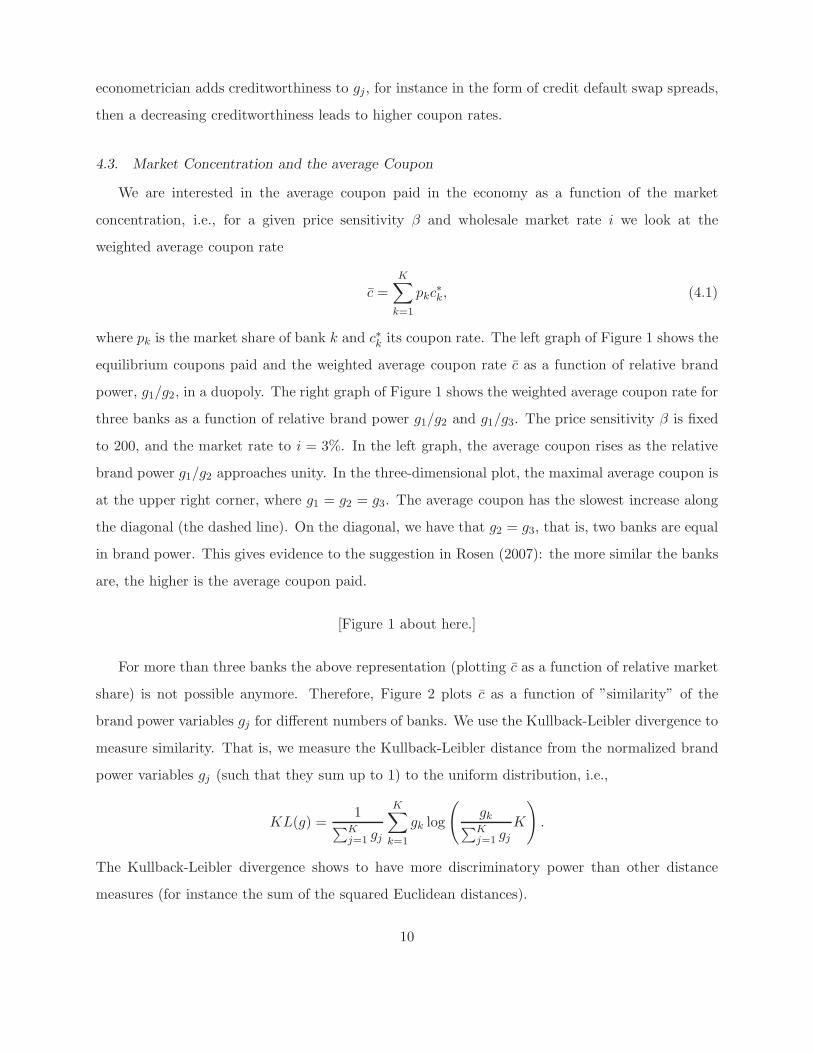
4.3. Market Concentration and the average Coupon

We are interested in the average coupon paid in the economy as a function of the market

concentration, i.e., for a given price sensitivity β and wholesale market rate i we look at the

weighted average coupon rate

c =K∑

k=1

pkc∗k, (4.1)

where pk is the market share of bank k and c∗k its coupon rate. The left graph of Figure 1 shows the

equilibrium coupons paid and the weighted average coupon rate c as a function of relative brand

power, g1/g2, in a duopoly. The right graph of Figure 1 shows the weighted average coupon rate for

three banks as a function of relative brand power g1/g2 and g1/g3. The price sensitivity β is fixed

to 200, and the market rate to i = 3%. In the left graph, the average coupon rises as the relative

brand power g1/g2 approaches unity. In the three-dimensional plot, the maximal average coupon is

at the upper right corner, where g1 = g2 = g3. The average coupon has the slowest increase along

the diagonal (the dashed line). On the diagonal, we have that g2 = g3, that is, two banks are equal

in brand power. This gives evidence to the suggestion in Rosen (2007): the more similar the banks

are, the higher is the average coupon paid.

[Figure 1 about here.]

For more than three banks the above representation (plotting c as a function of relative market

share) is not possible anymore. Therefore, Figure 2 plots c as a function of ”similarity” of the

brand power variables gj for different numbers of banks. We use the Kullback-Leibler divergence to

measure similarity. That is, we measure the Kullback-Leibler distance from the normalized brand

power variables gj (such that they sum up to 1) to the uniform distribution, i.e.,

KL(g) =1

∑Kj=1 gj

K∑

k=1

gk log

(gk∑Kj=1 gj

K

).

The Kullback-Leibler divergence shows to have more discriminatory power than other distance

measures (for instance the sum of the squared Euclidean distances).

10

[Figure 2 about here.]

Figure 2 confirms for 3, 5 and 7 banks, that the more similar the banks are, the higher is the

average coupon paid. Neuberger and Zimmerman (1990) search an explanation to the persistently

lower rates on deposits in the late eighties in California compared to the rest of the United States.

They find by statistical analysis that the lower rates can partially be explained by higher market

concentration. Our model supports this statistical finding, since higher market concentration leads

to lower coupon rates.

5. MULTI-PERIOD

In this Section, we extend our model to a multi-period economy. A multi-period optimizer sets

the same prices as a one-period optimizer. In the second part of this section, we approximate our

model by means of Taylor series. These approximations make it possible to compare our model

to the common models in the banking literature, on one hand, and to models used in Industrial

Organization theory on the other hand.

We define a closed, discrete time economy with dates t ∈ 0, 1, ..., τ. We want to invest in a

one-period riskless security, and rollover the investment. The riskless security worth 1 consumption

unit today is worth er(0) consumption units in the next period, where r(t) is the risk-free rate of

interest. At the end of the second period, the investment is worth er(0)+r(1).

By the risk neutral valuation principle, the price of a security satisfies the no arbitrage condition

if and only if there exists a probability measure Q, equivalent to the real-world measure, such that

under Q, the price process is a martingale, see Harrison and Kreps (1979).

Let (Ω,F , Fτt=0, Q) be a probability space, equipped with the finite filtration F0 ⊂ F1 ⊂ ... ⊂

Fτ . The price of the riskless security with remaining time to maturity T at time t is given by the

expected value under Q of the discounted consumption unit:

BT (t) = EQ[e−∑t+T−1

j=t r(j)|Ft]. (5.1)

Analogous, the present value of the deposit account for bank j is the expected value of the sum

of the discounted cash flows under the appropriate measure Q. The basic structure is the same

as in Jarrow and van Deventer (1998). The cash flows consist of volume increases minus coupon

11

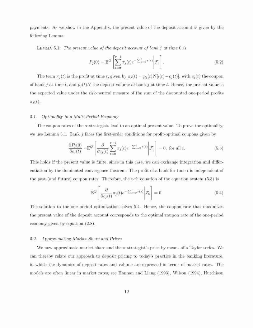
payments. As we show in the Appendix, the present value of the deposit account is given by the

following Lemma.

Lemma 5.1: The present value of the deposit account of bank j at time 0 is

Pj(0) = EQ

[τ−1∑

t=0

πj(t)e−∑t

s=0 r(s)

∣∣∣∣∣F0

]

. (5.2)

The term πj(t) is the profit at time t, given by πj(t) = pj(t)N [i(t)−cj(t)], with cj(t) the coupon

of bank j at time t, and pj(t)N the deposit volume of bank j at time t. Hence, the present value is

the expected value under the risk-neutral measure of the sum of the discounted one-period profits

πj(t).

5.1. Optimality in a Multi-Period Economy

The coupon rates of the α-strategists lead to an optimal present value. To prove the optimality,

we use Lemma 5.1. Bank j faces the first-order conditions for profit-optimal coupons given by

∂Pj(0)

∂cj(t)=EQ

[∂

∂cj(t)

τ−1∑

t=0

πj(t)e−∑t

s=0 r(s)

∣∣∣∣∣F0

]= 0, for all t. (5.3)

This holds if the present value is finite, since in this case, we can exchange integration and differ-

entiation by the dominated convergence theorem. The profit of a bank for time t is independent of

the past (and future) coupon rates. Therefore, the t-th equation of the equation system (5.3) is

EQ

[∂

∂cj(t)πj(t)e

−∑t

s=0 r(s)

∣∣∣∣∣F0

]= 0. (5.4)

The solution to the one period optimization solves 5.4. Hence, the coupon rate that maximizes

the present value of the deposit account corresponds to the optimal coupon rate of the one-period

economy given by equation (2.8).

5.2. Approximating Market Share and Prices

We now approximate market share and the α-strategist’s price by means of a Taylor series. We

can thereby relate our approach to deposit pricing to today’s practice in the banking literature,

in which the dynamics of deposit rates and volume are expressed in terms of market rates. The

models are often linear in market rates, see Hannan and Liang (1993), Wilson (1994), Hutchison

12

and Pennacchi (1996), Jarrow and van Deventer (1998), the Office of Thrift Supervision (2001),

and Kalkbrener and Willing (2004), for examples of both, linear and non-linear functions.

Using a Taylor series, the coupon rate c∗j of the α-strategist is, up to a first-order approximation,

c∗j (i, c0, ..., cj−1, cj+1, cK ; g0, ..., gj−1, gj+1, ..., gK ) ≈ c∗j (0) + i∂c∗j∂i

(0) +∑

k 6=j

ck

∂c∗j∂ck

(0), (5.5)

where the pricing formula c∗j (0) and the derivatives are evaluated at zero (i = 0, ck = 0 for all

banks). Since the function evaluations are constants, the approximated pricing formula (5.5) is a

linear function of the wholesale market rate and the competing banks’ prices. If the competing

banks set prices based on moving averages of wholesale market rates with different maturities, as

in Wilson (1994), we can replace the coupon rates ck in (5.5) by these moving averages. Then, the

α-strategist’s approximated coupon rate can be written as a linear function of wholesale market

rates as the only stochastic component.

Now, we consider the volume of the deposit account, which is Npj, with pj given by (2.5).

Omitting the time index, the logarithm of the volume deposited at bank j is

log Vj = log N + log gj + βcj − log

(∑

k

gkeβck

). (5.6)

Again, we approximate the above equation with a first-order Taylor series around zero and combine

constant terms to get

log Vj =νj0 +∑

k

νjkck + uj, (5.7)

where νjk are constants specific to bank j, and uj is an error term. If the competing banks’ prices

ck are functions of wholesale market rates, then we replace the coupons ck by these functions. In

consequence, the resulting volume model (5.7) is a function of wholesale market rates only, as the

common valuation models in the banking literature.

The coefficients of the volume model (5.7) and the coupon rate model (5.5) depend on the

brand powers, pricing strategies, and the depositor’s price sensitivity. To illustrate this, consider a

market with K banks, banks k = 1...n are short rate strategists, the remaining banks are replicating

strategists. Now, we write the volume model (5.7) as a function of the two different coupon rates.

The coefficient ν11 in the volume model is the coefficient for the coupon of the short rate strategist

13

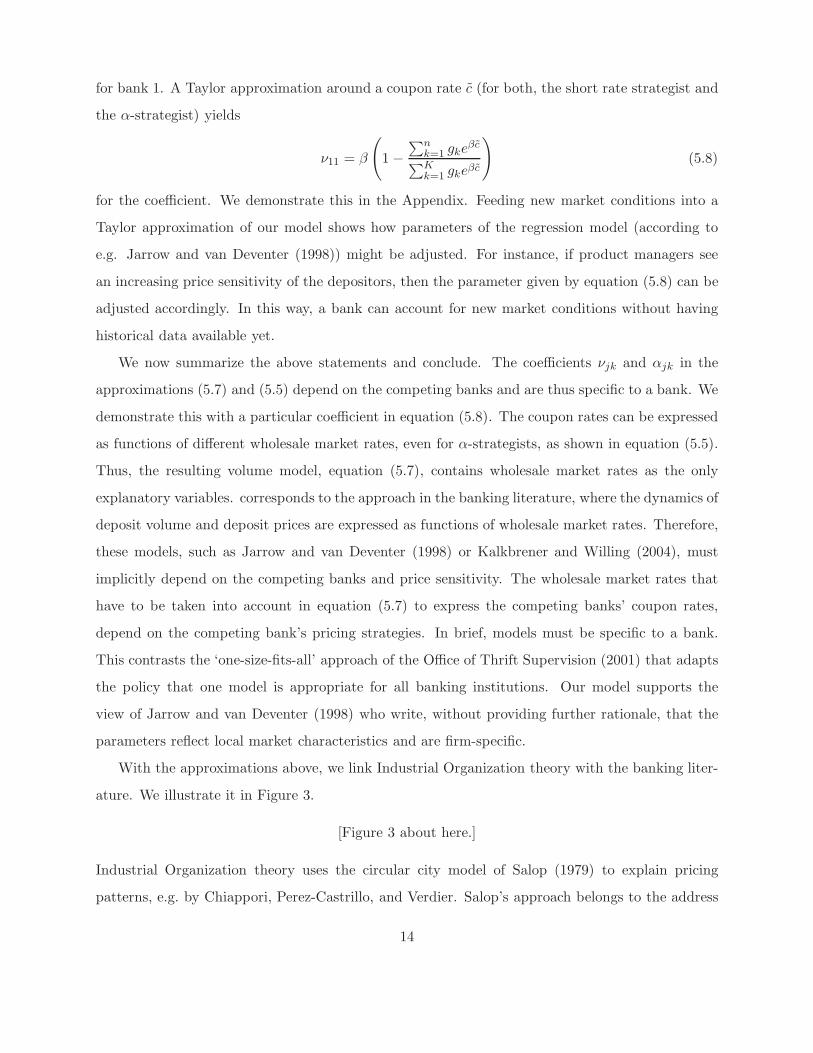
for bank 1. A Taylor approximation around a coupon rate c (for both, the short rate strategist and

the α-strategist) yields

ν11 = β

(

1 −∑n

k=1 gkeβc

∑Kk=1 gkeβc

)

(5.8)

for the coefficient. We demonstrate this in the Appendix. Feeding new market conditions into a

Taylor approximation of our model shows how parameters of the regression model (according to

e.g. Jarrow and van Deventer (1998)) might be adjusted. For instance, if product managers see

an increasing price sensitivity of the depositors, then the parameter given by equation (5.8) can be

adjusted accordingly. In this way, a bank can account for new market conditions without having

historical data available yet.

We now summarize the above statements and conclude. The coefficients νjk and αjk in the

approximations (5.7) and (5.5) depend on the competing banks and are thus specific to a bank. We

demonstrate this with a particular coefficient in equation (5.8). The coupon rates can be expressed

as functions of different wholesale market rates, even for α-strategists, as shown in equation (5.5).

Thus, the resulting volume model, equation (5.7), contains wholesale market rates as the only

explanatory variables. corresponds to the approach in the banking literature, where the dynamics of

deposit volume and deposit prices are expressed as functions of wholesale market rates. Therefore,

these models, such as Jarrow and van Deventer (1998) or Kalkbrener and Willing (2004), must

implicitly depend on the competing banks and price sensitivity. The wholesale market rates that

have to be taken into account in equation (5.7) to express the competing banks’ coupon rates,

depend on the competing bank’s pricing strategies. In brief, models must be specific to a bank.

This contrasts the ‘one-size-fits-all’ approach of the Office of Thrift Supervision (2001) that adapts

the policy that one model is appropriate for all banking institutions. Our model supports the

view of Jarrow and van Deventer (1998) who write, without providing further rationale, that the

parameters reflect local market characteristics and are firm-specific.

With the approximations above, we link Industrial Organization theory with the banking liter-

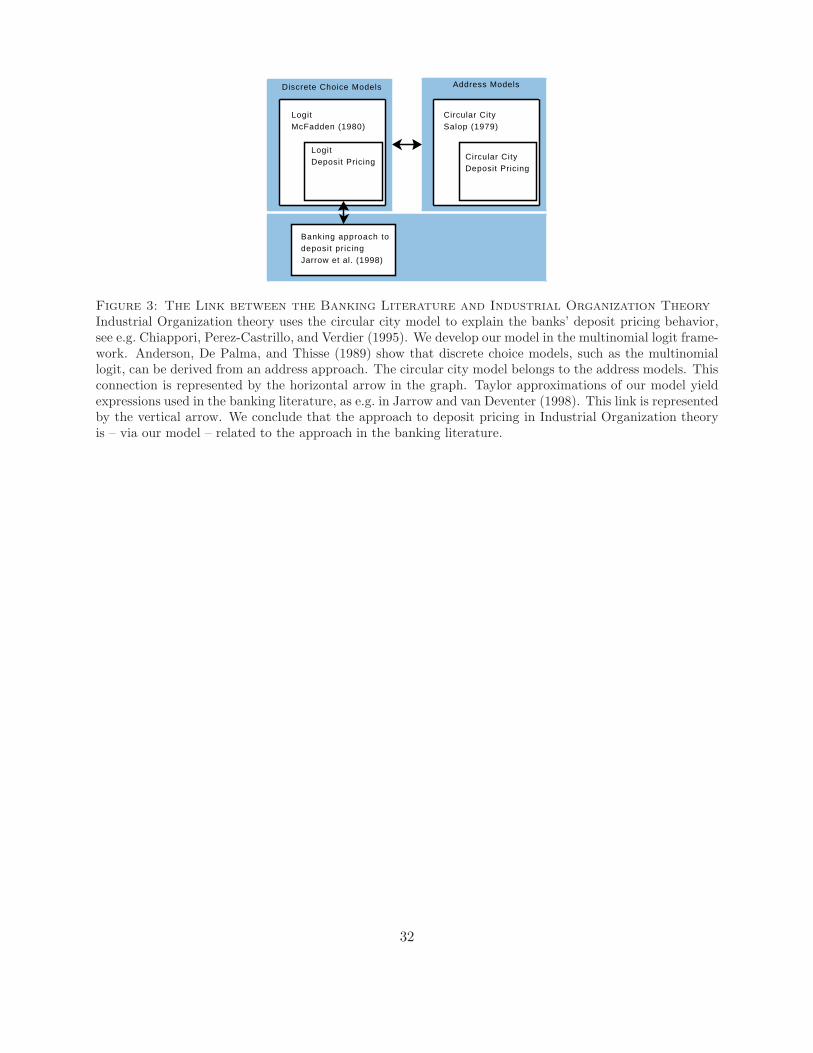
ature. We illustrate it in Figure 3.

[Figure 3 about here.]

Industrial Organization theory uses the circular city model of Salop (1979) to explain pricing

patterns, e.g. by Chiappori, Perez-Castrillo, and Verdier. Salop’s approach belongs to the address

14

models, while we develop our model in the discrete choice framework. The address approach is

connected to the discrete choice approach as shown by Anderson, De Palma, and Thisse (1989),

thereby our model is linked to Industrial Organization theory. Approximations of our model provide

the link to models employed in the banking literature (such as in Jarrow and van Deventer (1998)).

This closes the link between Industrial Organization theory and the banking literature.

In the next Section, we compare the performance of the α-strategists to other strategists. After

this, we compute the error emerging when present values are computed using the approximated

volume model (5.7).

6. SIMULATION

To compute the present value of a savings deposit account according to equation (5.2), we need

to describe the evolution of the interest rates. The short rate follows the time-discrete process

r(t) = a + br(t − 1) + ε(t), with ε(t)∼N(0, σ2

), |b| < 1, (6.1)

a discrete version of the Vasicek (1977) one-factor short rate model. The discretization unit is

one month, t + 1 is one month from t. The parameters we choose for the short rate model are

a/(1 − b) = 5.5%, b = 0.95, σ = 0.007/√

12, r(0) = 2.5%.

Banks are either α-strategists, equation (2.8), replicating strategists, or short rate strategists,

as described in the sequel. The practitioner’s approach to the replicating portfolio method is to

assume 20 percent of the deposits is highly volatile, while the remaining 80 percent are more stable,

see Wolff (2000). In this sense, we choose a replicating portfolio consisting of 20 percent 1-month

tranches and of 80 percent 5-year tranches. The resulting coupon rate of the replicating strategist

is then the weighted average of the one month rate and the moving average of 5 · 12 five year rates:

crep(t) =0.2i(t) + 0.81

60

t∑

j=t−59

i60M (j)

− M1, (6.2)

where the variable i60M is the wholesale market rate with a maturity of five years, M1 is a constant

spread. To compute (6.2), we need the closed-form solution for the zero bond yield with a maturity

of 60 months. We provide the solution in the Appendix. The short rate strategists price their

15

deposits according to Jarrow and van Deventer (1998), equation 8b of their publication, where the

coupon rate equals the wholesale market rate i minus a constant spread:

csr(t) =i(t) − M2. (6.3)

To ensure that the replicating strategists and the short rate strategists have similar chances of

profit, we choose the constant margins M1 and M2 such that both pay the same coupon rate

in average (over time). The α-strategists use the profit maximizing coupon, i.e., the fixed point

solution to equation (2.8).

6.1. Valuing different Strategists

We show the simulation results for different price strategists having identical brand power. To

compare the performance of the competing banks, we compute the present value of the deposit

accounts, integrated over state r(0):

P = EQ

[τ−1∑

t=0

πj(t)e−∑t

s=0 r(s)

]. (6.4)

To integrate over state, we allow the economy to adjust for 180 periods. We hold the market

volume N constant, this implies that depositors consume the coupon payments. We integrate over

time (τ = 5 years) and state (5000 paths) to compute the present value P . Figure 4 depicts the

simulation results, it shows expected coupons, and the present value of margin income as a function

of price sensitivity.

[Figure 4 about here.]

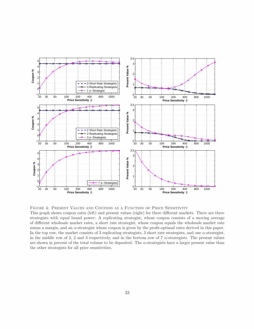
Present values of the short rate strategists and replicating strategists are close to the optimal

present value for certain price sensitivities β. This confirms the statement of Section 5.2, that

profit-optimal rates can be approximated with a function of market rates only. The coupons of

the α-strategists are low, if the price sensitivity is low. For increasing price sensitivities the curve

approaches the maximal coupon in the economy. In a market consisting of α-strategists only, the

present values collapse for high price sensitivities, since with increasing β, margins tend to zero,

as seen in Section 3.2. In the presence of only one α-strategist, his price reaches a maximum and

then decreases as β increases. This is not possible in the presence of several α-strategist, where the

price increases in β.

16

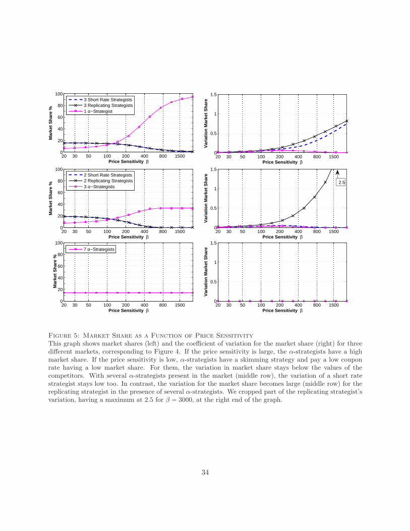
Figure 5 shows the market share and the coefficient of variation for the market share for different

strategists. Comparing the corresponding graphs of Figure 4 and Figure 5 shows that α-strategists

have a skimming strategy if price sensitivities remain low. That is, they have a low market share

and pay low coupon rates. With high price sensitivities their strategy is different, they have a large

market share and low margins.

[Figure 5 about here.]

The coefficient of variation for the market share stays relatively low for α-strategists for all

price sensitivities, whereas the conservative replicating strategists suffer from the quick reactions of

α-strategists. A short rate strategist can be viewed as the outside good in which the opportunity

rate equals the wholesale market rate minus a margin. Interestingly, the short rate strategist’s

coefficient of variation is low in the presence of several α-strategists and few other strategists. This

can possibly be explained by Proposition 3.2: α-strategists are short rate strategists if the market

consists only of α-strategists. If there are many α-strategists in the market, the pricing behavior is

dominated by them and their strategy is much like a short rate strategy. In consequence, the short

rate strategist that pays the α-strategists’ price plus a spread, has a coefficient of variation close

to the α-strategist.

6.2. Can we compute Present Values without considering the Competitors?

In Section 5.2 we showed that the deposit volume Npj of a bank, can be approximated in terms

of wholesale market rates. In this Section, we calculate present values of a short-rate strategist,

replacing the volume by the approximation given by (5.7). Omitting the index for bank j, the

approximation for a market with short rate strategists, replicating strategists, and α-strategists is

log(V (t)) = ν0 + ν1csr(t) + ν2crep(t) + u(t), (6.5)

with csr the coupon rate of the short rate strategist given by equation (6.3), crep that of a replicating

strategist given by equation (6.2). We assume u(t) to be an autocorrelated error, as in Janosi,

Jarrow, and Zullo (1999). That is, u(t) = ρu(t − 1) + ε(t), with i.i.d. normal ε(t), having mean

0 and variance σ2u, and u(0) = 0. In a first stage, we estimate the parameters νk, ρ, σ2

u of the

volume model (6.5), with the market share pj as dependent variable (using 6000 time steps and

17

averaging over 3000 paths). In a second stage, we calculate the present value P , equation (6.4),

and the resulting present value with the approximated volume model (6.5), i.e.,

P = EQ

[τ−1∑

t=0

V (t)(i(t) − csr(t))e−∑t

s=0 r(s)

]

, (6.6)

with V (t) given by equation (6.5) and csr the coupon rate of the short rate strategist given by

equation (6.3). The simulation horizon is 5 · 12 months. The error is (P − P )/P , with P given by

equation (6.4). We consider two different markets, both seen in Section 6.1. The first with 1 α-

strategist, 3 short rate strategists, and 3 replicating strategists and the second with 3 α-strategist,

2 short rate strategists, and 2 replicating strategists. Table A displays the percentage error. Note

that coupon rates, present values, market share, and the variation in market share for the scenarios

presented in Table A are displayed in Figure 4 and Figure 5.

[Table 1 about here.]

A short rate strategist that calculates the present value using the approximated volume model

given by equation (6.6) overestimates the value by about 2%. Table A also displays the estimated

parameters for the volume model. The intercept ν0 is decreasing with increasing price sensitivity.

The parameter ν3 is negative, because the short rate strategist’s market share profits from low rates

of the replicating strategist. The parameter ν1 is positive, because the short rate strategist gets more

volume if he pays higher coupon rates. We’re left to explain the size of the parameters ν1 and ν2.

In a market with 3 replicating strategists and 3 short rate strategists only, a Taylor approximation

shows that the coefficients ν1 and ν2 for the coupon rates are increasing in β (in absolute terms).

In fact we have already done this approximation for ν1 in equation (5.8), ν1 ≈ β(1 − 3/6) = β/2.

With only one α-strategist, as in the upper part of the Table, this pattern still holds. If there are

several α-strategists in the market, as in the lower part of the Table, the estimates show a u-shaped

pattern and are less straight forward to explain. We can see in the corresponding graph of Figure

5 (middle row) that the short rate strategist’s market share is almost zero for β = 800 and thus

the volume does not depend on the coupon rates anymore, so ν1 and ν2 are close to zero. If the

variation in market share is sufficiently large (see Figure 5), the error increases above 2%.

18

7. CONCLUSION

Industrial Organization theory provides models that explain banks’ deposit pricing decisions,

whereas in the banking literature, corresponding models are used to consider the risk and value of

deposit accounts. So far, these two streams have remained unrelated. If Industrial Organization

theory tells us that market conditions are crucial to the banks’ profit-optimal prices and deposit

volumes, this must somehow be incorporated in the valuation models. Otherwise the Asset-Liability

Management’s risk taking decisions, which are based on these valuations, are not as intended. We

show that the current valuation models implicitly account for local market conditions, since the

statistically estimated model parameters incorporate local market conditions. The consequence is

that the Asset-Liability Manager’s valuation models have to be reestimated on a regular basis to

account for changing market conditions.

There is no ‘one-size-fits-all’ approach to valuing deposits, meaning that models must be specific

to a bank. The Office of Thrift Supervision evaluates savings institutions’ interest rate risk by

estimating the sensitivity of their portfolio to changes in wholesale market rates. They provide a

model with parameters that differ among the type of the deposit account2 but not among banks.

Models must be bank-specific, these risk valuations and the resulting recommendations for the

thrift institutions may be seriously in error. The rationale for bank-specific models is that profit-

optimal deposit prices and deposit volumes depend on the competing banks’ prices and brand

powers. These quantities differ among markets and banks in a given market. Greater banks have

lower profit-optimal deposit rates and their pricing strategy has a large impact on the competing

banks’ optimal prices, hence: size matters.

19

A. PROOFS

Proof Of Equation (2.8), Profit Maximizing Coupon Rate. Maximizing the profit πj = Npj [i − cj ]

results in the first-order condition

0 =∂πj

∂cj= N

∂pj

∂cj[i − cj ] − Npj, (A.1)

with pj given by

pj =gje

βcj

∑Kk=1 gkeβck

. (A.2)

Now, the marginal increase in market share with a marginal increase in the coupon rate is given

by,

∂pj

∂cj=

gjecjββ

∑k 6=j gke

ckβ

[∑Kk=1 gkeckβ

]2 = βpj(1 − pj),

so that the first-order condition (A.1) for an optimal profit becomes

ecjβ = − 1

gjβ

∑

k 6=j

gkeckβ

[cj −

(i − 1

β

)]. (A.3)

The second derivative of the profit is

∂2πj

∂c2j

= (i − cj)Nβ2(1 − 2pj)pj(1 − pj) − 2Nβpj(1 − pj). (A.4)

Evaluating (A.4) at any point where the first-order condition (A.1) is met yields −Nβpj, which

is negative. Therefore the solution to the first-order condition indeed maximizes profit. To solve

equation (A.3) in cj we resort to the following Lemma that uses the Lambert W function (Corless,

Gonnet, Hare, Jeffrey, and Knuth 1996)

Lemma A.1: The solution to the transcendental algebraic equation in x of the form

e−a0x = a1 (x − b) (A.5)

with a0, a1, b ∈ R, has the solution x = b + 1a0

W(

a0a1

e−a0b)

where W (.) is the Lambert W function,

which is the inverse function of f(z) = zez with z ∈ C.

20

The proof of Lemma A.1 is straightforward, using the definition of the Lambert W function.

Equation A.5 can be restated a0/a1e−a0x = (x − b)a0, and then a0/a1e

−a0b = (x − b)a0e(x−b)a0 .

Applying the definition of W (.) yields the stated solution.

Hence, the solution to (A.3) is given by,

c∗j = i − 1

β

[1 + W

(gje

βi−1

∑k 6=j gkeckβ

)], (A.6)

when we replace a0, a1, and b in Lemma A.1 by

a0 = −β, b = i − 1

β, and a1 = − 1

gjβ∑

k 6=j

gkeckβ.

The arguments to W (.) are always positive and thus the solution is in R.

Proof Of Proposition 3.1, Unique Nash Equilibrium. Let M ≤ K be the number of α-strategists in

the economy. We define the coupon vector as c = (c1, . . . , cM )T . If M < K the coupons of the

K − M non α-strategists do not depend on the other banks’ coupons. Let C : RM → RM be the

mapping defined by applying c∗j , equation (A.6), to every coupon that belongs to an α-strategist.

Assume the initial coupon vector is c0 ∈ RM . When every bank j = 1, ...,M applies equation (A.6),

the coupon is c1 = C(c0). After two steps the coupon is c2 = C(c1) = C(C(c0)), et cetera. The

coupon vector obtained when t times applying the mapping C is ct. We define the mapping C as

C :

c1

...

cM

7→

i − 1β

[1 + W

(g1eβi−1

∑Kk=2 gkeckβ

)]

...

i − 1β

[1 + W

(gjeβi−1

∑Kk=1,k 6=j gkeckβ

)]

...

i − 1β

[1 + W

(gMeβi−1

∑Kk=1,k 6=M gkeckβ

)]

. (A.7)

The proof works as follows. We show that the infinity norm of the Jacobian of C is smaller

than one. Then, we derive an upper and a lower bound for the equilibrium coupons. We then can

apply Theorem 5.4.1 in Judd (1998).

21

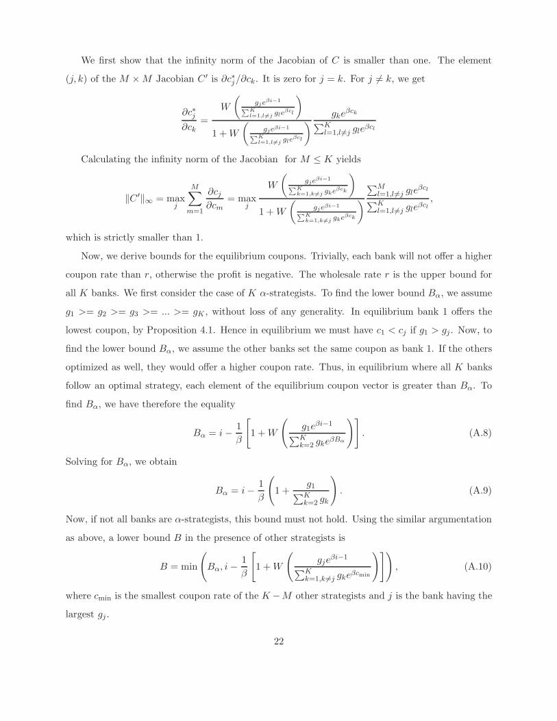
We first show that the infinity norm of the Jacobian of C is smaller than one. The element

(j, k) of the M × M Jacobian C ′ is ∂c∗j/∂ck. It is zero for j = k. For j 6= k, we get

∂c∗j∂ck

=

W

(gjeβi−1

∑Kl=1,l6=j gle

βcl

)

1 + W

(gjeβi−1

∑Kl=1,l6=j gle

βcl

) gkeβck

∑Kl=1,l 6=j gleβcl

Calculating the infinity norm of the Jacobian for M ≤ K yields

‖C ′‖∞ = maxj

M∑

m=1

∂cj

∂cm

= maxj

W

(gjeβi−1

∑Kk=1,k 6=j gkeβck

)

1 + W

(gjeβi−1

∑Kk=1,k 6=j gkeβck

)∑M

l=1,l 6=j gleβcl

∑Kl=1,l 6=j gleβcl

,

which is strictly smaller than 1.

Now, we derive bounds for the equilibrium coupons. Trivially, each bank will not offer a higher

coupon rate than r, otherwise the profit is negative. The wholesale rate r is the upper bound for

all K banks. We first consider the case of K α-strategists. To find the lower bound Bα, we assume

g1 >= g2 >= g3 >= ... >= gK , without loss of any generality. In equilibrium bank 1 offers the

lowest coupon, by Proposition 4.1. Hence in equilibrium we must have c1 < cj if g1 > gj . Now, to

find the lower bound Bα, we assume the other banks set the same coupon as bank 1. If the others

optimized as well, they would offer a higher coupon rate. Thus, in equilibrium where all K banks

follow an optimal strategy, each element of the equilibrium coupon vector is greater than Bα. To

find Bα, we have therefore the equality

Bα = i − 1

β

[1 + W

(g1e

βi−1

∑Kk=2 gkeβBα

)]. (A.8)

Solving for Bα, we obtain

Bα = i − 1

β

(

1 +g1∑K

k=2 gk

)

. (A.9)

Now, if not all banks are α-strategists, this bound must not hold. Using the similar argumentation

as above, a lower bound B in the presence of other strategists is

B = min

(Bα, i − 1

β

[1 + W

(gje

βi−1

∑Kk=1,k 6=j gkeβcmin

)]), (A.10)

where cmin is the smallest coupon rate of the K −M other strategists and j is the bank having the

largest gj .

22

We can choose any Bl, Bu ∈ R such that Bl < B and Bu > i. Altogether, we have a differentiable

contraction map on [Bl, Bu]M , since it is a closed, bounded, convex set and the matrix norm of

the Jacobi matrix is strictly smaller than one, we can apply Theorem 5.4.1 in Judd (1998), the

sequence defined by ct+1 = C(ct) converges to c∗.

Proof Of Proposition 3.2. Solving the first-order condition of the profit N∂pj/∂cj [i − cj ]−Npj = 0,

for β(i − cj) yields 1/(1 − pj), or

∑k gke

βck

∑k 6=j gkeβck

= β(i − cj) (A.11)

using c∗j = i − mj/β for the α-strategists, we can state

g0eβc0 +

∑Kk=1 gke

βi−mk

g0eβc0 +∑K

k=1,k 6=j gkeβi−mk

=mj.

This can be rewritten as

e−mj =

g0

gjeβ(c0−i) +

∑

k 6=j

gk

gje−mk

(mj − 1).

Using Lemma A.1 with a0 = 1, a1 = g0

gjeβ(c0−i) +

∑k 6=j

gk

gje−mk , b = 1, we obtain

mj = 1 + W

(gj

g0eβc0e1−βi +∑

k 6=j gke1−mk

)

, j = 1...K,

completing the proof.

Proof Of Proposition 4.1. A bank with a greater brand power has a lower optimal coupon. This

can be proven by contradiction. Bank j has brand power gj , bank m brand power gm and gj > gm.

Assume bank j offers a lower coupon than bank m. From gm > gj and cm ≥ cj , it follows

gmeβi−1

gjeβcj + G>

gjeβi−1

gmeβcm + G, (A.12)

with G =∑K

k,k 6=j,m gkeβck . Applying the pricing formula (A.6) we obtain cm < cj which contradicts

our earlier assumption that in equilibrium cm ≥ cj . Hence in equilibrium we must have cm < cj if

gm > gj .

23

Proof Of Lemma 5.1, Present Value Of The Deposit Account. The present value of the deposit ac-

count is the sum of the discounted cash flows under the risk neutral measure Q. The deposit volume

of bank j at time t is abbreviated by V (t).

Pj(0) =EQ

[V (0) +

τ−2∑

t=0

(V (t + 1) − V (t))e−∑t

s=0 r(s) − V (τ − 1)e−∑t

s=0 r(s)

∣∣∣∣∣F0

]

− EQ

[τ−1∑

t=0

cj(t)V (t)e−∑t

s=0 r(s)

∣∣∣∣∣F0

]

=EQ

[

V (0) +

τ−2∑

t=0

V (t + 1)e−∑t+1

s=0 r(s)er(t+1) −τ−1∑

t=0

V (t)e−∑t

s=0 r(s)

∣∣∣∣∣F0

]

− EQ

[τ−1∑

t=0

cj(t)V (t)e−∑t

s=0 r(s)

∣∣∣∣∣F0

]

=EQ

[τ−1∑

t=0

V (t)e−∑t

s=0 r(s)er(t) −τ−1∑

t=0

V (t)e−∑t

s=0 r(s)

∣∣∣∣∣F0

]

− EQ

[τ−1∑

t=0

cj(t)V (t)e−∑t

s=0 r(s)

∣∣∣∣∣F0

]

We use the equivalence er(t) = 1 + i(t), to get

Pj(0) =EQ

[τ−1∑

t=0

V (t)(i(t) − cj(t))e−∑t

s=0 r(s)

∣∣∣∣∣F0

]

(A.13)

=EQ

[τ−1∑

t=0

πj(t)e−∑t

s=0 r(s)

∣∣∣∣∣F0

]. (A.14)

Hence, the present value of the deposit account reduces to the expected value of the sum of the

discounted one period profits.

Derivation Of The Bond Price. If the short rate follows the time-discrete process

r(t) = a + br(t − 1) + ε(t), with ε(t)∼N(0, σ2

), |b| < 1, and t ∈ N, (A.15)

the closed-form solutions for the price of the zero bond and the zero bond yield at time t with

remaining time to maturity T ∈ N are given by

BT (t) = exp

−mT (t) +

1

2vT

and rT (t) =

1

T

mT (t) − 1

2vT

, (A.16)

24

where

mT (t) = r(t)1 − bT

1 − b+ a

(T − 1

1 − b− b

1 − bT−1

(1 − b)2

)(A.17)

vT = σ2

(T − 1

(1 − b)2− 2b

1 − bT−1

(1 − b)3+ b2 1 − b2(T−1)

(1 + b)(1 − b)3

)

. (A.18)

We obtain by iteration of equation (A.15),

r(t) =t−1∑

j=0

bj (a + εt−j) + btr(0).

Today’s price (t = 0) of a bond paying a sure dollar in time T is given by BT (0) = EQ[e−∑T−1

j=0 r(j)].

Since |b| < 1 by the properties of a geometric series,

T−1∑

t=0

r(t) =

T−1∑

t=1

t−1∑

j=0

bj (a + εt−j)

+ r(0)

T−1∑

t=0

bt

=

T−1∑

n=1

1 − bT−n

1 − b(a + εn) + r(0)

1 − bT

1 − b

=T−1∑

n=1

1 − bT−n

1 − bεn + a

(T − 1

1 − b− b

1 − bT−1

(1 − b)2

)+ r(0)

1 − bT

1 − b.

The first term on the last line is a sum of independent Gaussian variables and therefore Gaussian

as well. The mean of the first term is zero and the variance can be determined via expansion of a

geometric series,

T−1∑

n=1

(1 − bT−n

1 − b

)2

=T − 1

(1 − b)2− 2b

1 − bT−1

(1 − b)3+ b2 1 − b2(T−1)

(1 + b)(1 − b)3.

By the definitions of m(T ) and v(T ) in the Equations (A.17) and (A.18), we therefore have

T−1∑

t=0

r(t)∼N (m(T ), v(T )) .

The definition of the zero bond yield rT (0) := − 1T

log BT (0) = 1T

mT (0) − 1

2vT

as well as the

mean of the log-normal distribution, BT (t) = E

[exp(−∑t+T−1

j=t r(j))], complete the proof.

Taylor Approximation of the Volume Model, Derivation of Equation (5.8). Consider a market with

K banks. The first n banks are short rate strategists, the remaining banks are replicating strate-

25

gists. The logarithm of the volume of bank 1 is given by the logarithm of market share p1, equation

(2.5), times market volume N ,

log N + log p1 = log N + log g1 + βcsr − log

(n∑

k=1

gkeβcsr +

K∑

k=n+1

gkeβcrep

), (A.19)

where csr is the coupon rate of the short rate strategist, and crep the coupon rate of the replicating

strategist. The Taylor series approximation of the logarithm (containing the two sums) evaluated

at csr and crep is, up to first-order terms,

log(.) ≈ f0 +(csr − csr)β

∑nk=1 gke

βcsr

∑nk=1 gkeβcsr +

∑Kk=n+1 gkeβcrep

+(crep − crep)β

∑nk=1 gke

βcrep

∑nk=1 gkeβcsr +

∑Kk=n+1 gkeβcrep

,

where csr and crep are nearby coupon rates, f0 is the logarithm evaluated at crep, csr. Substituting

this Taylor approximation into (A.19), combining constant terms and rearranging, we can write

the equation as:

log N + log p1 ≈ν10 (A.20)

+ β

(1 −

∑nk=1 gke

βcsr

∑nk=1 gkeβcsr +

∑Kk=n+1 gkeβcrep

)csr (A.21)

+ β

∑nk=1 gke

βcrep

∑nk=1 gkeβcsr +

∑Kk=n+1 gkeβcrep

crep. (A.22)

The coefficient of the short rate strategist’s coupon rate is given by (A.21). We obtain equation

(5.8), when replacing csr and crep by c.

26

LITERATURE CITED

Anderson, S., and A. De Palma (1992): “The logit as a model of product differentiation,” Oxford

Economic Papers, 44(1), 51–67.

Anderson, S., A. De Palma, and J. Thisse (1989): “Demand for differentiated products, discrete

choice models, and the characteristics approach,” The Review of Economic Studies, 56(1), 21–

35.

Anderson, S., A. De Palma, and J. Thisse (2001): Discrete choice theory of product differentiation.

MIT press.

Bassett, W., and T. Brady (2002): “What drives the persistent competitiveness of small banks?,”

Finance and economics discussion series - Federal Reserve Board.

Chiappori, P.-A., D. Perez-Castrillo, and T. Verdier (1995): “Spatial competition in the banking

system: Localization, cross subsidies and the regulation of deposit rates,” European Economic

Review, 39(5), 889 – 918.

Corless, R. M., G. H. Gonnet, D. E. G. Hare, D. J. Jeffrey, and D. E. Knuth (1996): “On the

Lambert W function,” Advances in Computational Mathematics, 5, 329359.

De Palma, A., V. Ginsburgh, Y. Papageorgiou, and J. Thisse (1985): “The principle of minimum

differentiation holds under sufficient heterogeneity,” Econometrica, 53(4), 767–781.

Frauendorfer, K., and M. Schurle (2003): “Management of non-maturing deposits by multistage

stochastic programming,” European Journal of Operational Research, 151(3), 602–616.

Freixas, X., and J. Rochet (1999): Microeconomics of banking. MIT press.

Gambacorta, L. (2008): “How do banks set interest rates?,” European Economic Review, 52(5),

792–819.

Hannan, T., and A. Berger (1991): “The rigidity of prices: Evidence from the banking industry,”

The American Economic Review, 81(4), 938–945.

Hannan, T., and J. Liang (1993): “Inferring market power from time-series data: The case of the

banking firm,” International Journal of Industrial Organization, 11(2), 205–218.

27

Harrison, J., and D. Kreps (1979): “Martingales and arbitrage in multiperiod securities markets,”

Journal of economic theory, 20(3), 381–408.

Hutchison, D., and G. Pennacchi (1996): “Measuring rents and interest rate risk in imperfect fi-

nancial markets: The case of retail bank deposits,” The Journal of Financial and Quantitative

Analysis, 31(3), 399–417.

Janosi, T., R. Jarrow, and F. Zullo (1999): “An empirical analysis of the Jarrow-van Deventer

model for valuing non-maturity demand deposits,” The Journal of Derivatives, 7(1), 8–31.

Jarrow, R. A., and D. R. van Deventer (1998): “The arbitrage-free valuation and hedging of de-

mand deposits and credit card loans,” Journal of Banking & Finance, 22(3), 249–272.

Judd, K. (1998): Numerical methods in economics. The MIT Press.

Kalkbrener, M., and J. Willing (2004): “Risk management of non-maturing liabilities,” Journal of

Banking and Finance, 28(7), 1547–1568.

Klein, M. (1971): “A theory of the banking firm,” Journal of Money, Credit and Banking, 3(2),

205–218.

Luce, R., and P. Suppes (1965): “Preference, utility, and subjective probability,” Handbook of

mathematical psychology, 3, 249–410.

Manski, C., and D. McFadden (1983): Structural analysis of discrete data with econometric appli-

cations. MIT Press Cambridge, MA.

Martın-Oliver, A., V. Salas-Fumas, and J. Saurina (2007): “A test of the law of one price in retail

banking,” Journal of Money, Credit and Banking, 39(8), 2021–2040.

McFadden, D. (1980): “Econometric models for probabilistic choice among products,” The Journal

of Business, 53(3), 13–29.

McFadden, D. (1986): “The choice theory approach to market research,” Marketing Science, 5(4),

275–297.

Monti, M. (1972): “Deposit, credit, and interest rate determination under alternative bank objec-

tives,” Mathematical Methods in Investment and Finance, pp. 431–454.

28

Neuberger, J. A., and G. C. Zimmerman (1990): “Bank pricing of retail deposit accounts and ’the

California rate mystery’,” Economic Review (Federal Reserve Bank of San Francisco), 0(2), 3–16.

Office of Thrift Supervision (2001): Net Portfolio Value Model Manual, Section 6.D.

Park, K., and G. Pennacchi (2008): “Harming depositors and helping borrowers: The disparate

impact of bank consolidation,” Review of Financial Studies.

Pita Barros, P. (1999): “Multimarket competition in banking, with an example from the Portuguese

market,” International Journal of Industrial Organization, 17(3), 335–352.

Rosen, R. J. (2007): “Banking market conditions and deposit interest rates,” Journal of Banking

& Finance, 31(12), 3862 – 3884.

Salop, S. (1979): “Monopolistic competition with outside goods,” The Bell Journal of Economics,

pp. 141–156.

The Federal Reserve Board (2009): Consumer Compliance Handbook, Deposit-Related Regulations

and Statutes, Regs. Q and D.

Vasicek, O. (1977): “An equilibrium characterization of the term structure,” Journal of Financial

Economics, 5(2), 177–188.

Wilson, T. (1994): “Optimal values,” Balance sheet, 3(3), 13–20.

Wolff, A. (2000): “Valuing non-maturity deposits: two alternative approaches,” Balance Sheet, 8.

Notes

1The density function is fGum(z; κ, 1) = e(κ−z)−eκ−z

, where κ is Euler’s constant (κ ≈ 0.5772). The scale-one

assumption of the Gumbel distribution is not crucial to our analysis. One could instead assume scale µ. The weights

γ and β in (2.3) would then be replaced by γ/µ and β/µ. This would not bring further insights into our analysis and

we thus choose µ = 1.

2The Office of Thrift Supervision (2001) provides models (including parameters) for transaction accounts, NOW,

Super NOW, and other interest-bearing transaction accounts.

29

0.20.4

0.60.8

1

0.2

0.4

0.6

0.8

10

0.5

1.0

1.5

2.0

2.5

g1/g

3

3 Banks

g1/g

2

Co

up

on

%

0 0.2 0.4 0.6 0.8 1−0.5

0

0.5

1.0

1.5

2.0

2.5

Relative Brand Power g1/g

2

Co

up

on

%

2 Banks

Weighted Average CouponEquilibrium Coupon Bank 1Equilibrium Coupon Bank 2

Figure 1: Equilibrium Coupon Rates as a Function of Relative Brand Power

This Figure shows the average coupon weighted by market share as a function of relative brand power for twobanks (left) and three banks (right). Hence, the dashed line for two banks on the left plot corresponds to thesurface for three banks on the right plot. The maximal average coupon rate is paid if banks have an equalbrand power. The more the banks differ, the lower is the average coupon paid. In the three-dimensionalplot, the average coupon has the slowest decrease along the dashed diagonal. On the diagonal, bank 2 andbank 3 are equal in brand power.

30

0 0.5 1.0 1.5 2.00.5

1.0

1.5

2.0

2.5

KL Distance To The Uniform Distribution

Co

up

on

%

3 Banks

0 0.5 1.0 1.5 2.00.5

1.0

1.5

2.0

2.5

KL Distance To The Uniform DistributionC

ou

po

n %

5 Banks

0 0.5 1.0 1.5 2.00.5

1.0

1.5

2.0

2.5

KL Distance To The Uniform Distribution

Co

up

on

%

7 Banks

0 0.5 1.0 1.5 2.00.5

1.0

1.5

2.0

2.5

KL Distance To The Uniform Distribution

Co

up

on

%

8 Banks

Figure 2: Equilibrium Coupon Rates as a Function of Similarity of the Banks

This Figure shows the average coupon weighted by market share, as in Figure 1, but here as a function ofsimilarity for 3, 5, 7, and 8 banks. The similarity is measured by means of the Kullback-Leibler distancebetween the brand power variables and the uniform distribution. The distance is zero if all banks are equalin brand power. The graphs show that the more similar the banks are, the higher is the average couponrate. We can directly compare the graph for 3 banks to the three-dimensional graph of Figure 1.

31

Address Models

Circular CitySalop (1979)

Circular CityDeposit Pricing

Discrete Choice Models

LogitMcFadden (1980)

LogitDeposit Pricing

Banking approach to deposit pricingJarrow et al. (1998)

Figure 3: The Link between the Banking Literature and Industrial Organization Theory

Industrial Organization theory uses the circular city model to explain the banks’ deposit pricing behavior,see e.g. Chiappori, Perez-Castrillo, and Verdier (1995). We develop our model in the multinomial logit frame-work. Anderson, De Palma, and Thisse (1989) show that discrete choice models, such as the multinomiallogit, can be derived from an address approach. The circular city model belongs to the address models. Thisconnection is represented by the horizontal arrow in the graph. Taylor approximations of our model yieldexpressions used in the banking literature, as e.g. in Jarrow and van Deventer (1998). This link is representedby the vertical arrow. We conclude that the approach to deposit pricing in Industrial Organization theoryis – via our model – related to the approach in the banking literature.

32

20 30 50 100 200 400 800 1500−1

0

1

2

3

4

5

Co

up

on

%

Price Sensitivity β

20 30 50 100 200 400 800 15000

1

2

3

3.5

Pre

sen

t V

alu

e %

Price Sensitivity β

20 30 50 100 200 400 800 1500−1

0

1

2

3

4

5

Co

up

on

%

Price Sensitivity β

20 30 50 100 200 400 800 15000

1

2

3

3.5

Pre

sen

t V

alu

e %

Price Sensitivity β

20 30 50 100 200 400 800 1500−1

0

1

2

3

4

5

Co

up

on

%

Price Sensitivity β

20 30 50 100 200 400 800 15000

1

2

3

3.5

Pre

sen

t V

alu

e %

Price Sensitivity β

3 Short Rate Strategists3 Replicating Strategists1 α−Strategist

2 Short Rate Strategists2 Replicating Strategists3 α−Strategists

7 α−Strategists

Figure 4: Present Values and Coupons as a Function of Price Sensitivity

This graph shows coupon rates (left) and present values (right) for three different markets. There are threestrategists with equal brand power: A replicating strategist, whose coupon consists of a moving averageof different wholesale market rates, a short rate strategist, whose coupon equals the wholesale market rateminus a margin, and an α-strategist whose coupon is given by the profit-optimal rates derived in this paper.In the top row, the market consists of 3 replicating strategists, 3 short rate strategists, and one α-strategist,in the middle row of 2, 2 and 3 respectively, and in the bottom row of 7 α-strategists. The present valuesare shown in percent of the total volume to be deposited. The α-strategists have a larger present value thanthe other strategists for all price sensitivities.

33

20 30 50 100 200 400 800 15000

20

40

60

80

100

Mar

ket

Sh

are

%

Price Sensitivity β

20 30 50 100 200 400 800 15000

0.5

1

1.5

Var

iati

on

Mar

ket

Sh

are

Price Sensitivity β

20 30 50 100 200 400 800 15000

20

40

60

80

100

Mar

ket

Sh

are

%

Price Sensitivity β

20 30 50 100 200 400 800 15000

0.5

1

1.5

Var

iati

on

Mar

ket

Sh

are

Price Sensitivity β

20 30 50 100 200 400 800 15000

20

40

60

80

100

Mar

ket

Sh

are

%

Price Sensitivity β

20 30 50 100 200 400 800 15000

0.5

1

1.5

Var

iati

on

Mar

ket

Sh

are

Price Sensitivity β

3 Short Rate Strategists3 Replicating Strategists1 α−Strategist

2 Short Rate Strategists2 Replicating Strategists3 α−Strategists

7 α−Strategists

2.5

Figure 5: Market Share as a Function of Price Sensitivity

This graph shows market shares (left) and the coefficient of variation for the market share (right) for threedifferent markets, corresponding to Figure 4. If the price sensitivity is large, the α-strategists have a highmarket share. If the price sensitivity is low, α-strategists have a skimming strategy and pay a low couponrate having a low market share. For them, the variation in market share stays below the values of thecompetitors. With several α-strategists present in the market (middle row), the variation of a short ratestrategist stays low too. In contrast, the variation for the market share becomes large (middle row) for thereplicating strategist in the presence of several α-strategists. We cropped part of the replicating strategist’svariation, having a maximum at 2.5 for β = 3000, at the right end of the graph.

34

TABLE A

Present Value Errors in two different Markets.

Market Price Parameter Estimates of the Volume Model Relative

Structure Sensitivity β ν0 ν1 ν2 ρ σu Error

1α,3

Shor

tR

ate,

3R

eplica

ting 20 5.05 9.34 −9.35 0.88 0.01% 1.9%

30 5.04 13.94 −13.95 0.88 0.01% 1.9%

50 5.03 22.95 −22.98 0.88 0.04% 1.9%

100 4.98 44.28 −44.33 0.88 0.15% 1.9%

200 4.82 81.25 −81.23 0.88 0.54% 2.0%

400 4.34 149.82 −149.88 0.88 1.74% 2.1%

800 3.38 329.72 −329.04 0.88 6.46% 3.7%

1500 2.28 678.70 −677.37 0.88 19.30% 22.2%

3α,2

Shor

tR

ate,

2R

eplica

ting 20 5.25 7.73 −7.76 0.88 0.01% 1.9%

30 5.23 11.38 −11.41 0.88 0.01% 1.9%

50 5.18 18.19 −18.23 0.88 0.03% 1.9%

100 5.02 32.08 −32.13 0.88 0.13% 1.9%

200 4.57 45.77 −45.83 0.88 0.40% 1.9%

400 3.13 30.88 −30.98 0.88 0.67% 1.9%

800 −0.69 2.32 −2.46 0.85 0.16% 1.9%

1500 −7.69 −0.10 −0.02 0.75 0.01% 1.9%

Notes: This Table shows the present value errors for a short rate strategist in two different markets.Errors arise when we use an approximated volume model that ignores the competing banks. The error is(P − P )/P , where P is the present value and P the approximation of the present value. We obtain P byreplacing the volume of the replicating strategist by a Taylor approximation. The approximated volume isgiven by V (t) = exp (ν0 + ν1csr(t) + ν2crep(t) + u(t)) with u(t) = ρu(t− 1)+ ε(t). The error ε(t) is normallydistributed with mean zero and variance σ2

u. The variable crep is the coupon rate of a replicating strategist,

csr the coupon rate of a short rate strategist. For both markets and every price sensitivity, we estimate theparameters of the volume model (ν0, ν1, ν2, σu, and ρ). In a second simulation stage, we calculate P , and

P using these estimates. The error is around 2%. With few α-strategists in the market and very high pricesensitivities, the error increases.

35