optimal design of low-contrast two-phase structures for
TRANSCRIPT

HAL Id: hal-00784049https://hal.inria.fr/hal-00784049
Submitted on 4 Aug 2020
HAL is a multi-disciplinary open accessarchive for the deposit and dissemination of sci-entific research documents, whether they are pub-lished or not. The documents may come fromteaching and research institutions in France orabroad, or from public or private research centers.
L’archive ouverte pluridisciplinaire HAL, estdestinée au dépôt et à la diffusion de documentsscientifiques de niveau recherche, publiés ou non,émanant des établissements d’enseignement et derecherche français ou étrangers, des laboratoirespublics ou privés.
Optimal Design of Low-contrast Two-phase StructuresFor the Wave Equation
Grégoire Allaire, Alex Kelly
To cite this version:Grégoire Allaire, Alex Kelly. Optimal Design of Low-contrast Two-phase Structures For the WaveEquation. Mathematical Models and Methods in Applied Sciences, World Scientific Publishing, 2011,21 (7), pp.1499–1538. 10.1142/S0218202511005477. hal-00784049
ECOLE POLYTECHNIQUE
CENTRE DE MATHÉMATIQUES APPLIQUÉESUMR CNRS 7641
91128 PALAISEAU CEDEX (FRANCE). Tél: 01 69 33 46 00. Fax: 01 69 33 46 46
http://www.cmap.polytechnique.fr/
Optimal Design of Low-ContrastTwo Phase Structures for the
Wave Equation
Grégoire Allaire, Alex Kelly
R.I. 692 August 2010


Optimal Design of Low-Contrast Two Phase
Composites for Wave Propagation ∗
Grégoire Allaire and Alex KellyCMAP, Ecole Polytechnique91128 Palaiseau, FRANCE
([email protected], [email protected])
August 25, 2010
Abstract
This paper is concerned with the following optimal design problem: nd the distri-bution of two phases in a given domain that minimizes an objective function evaluatedthrough the solution of a wave equation. This type of optimization problem is known tobe ill-posed in the sense that it generically does not admit a minimizer among classicaladmissible designs. Its relaxation could be found, in principle, through homogenizationtheory but, unfortunately, it is not always explicit, in particular for objective func-tions depending on the solution gradient. To circumvent this diculty we make thesimplifying assumption that the two phases have a low constrast. Then, a second or-der asymptotic expansion with respect to the small amplitude of the phase coecientsyields a simplied optimal design problem which is amenable to relaxation by meansof H-measures. We prove a general existence theorem in a larger class of compositematerials and propose a numerical algorithm to compute minimizers in this context. Asin the case of an elliptic state equation, the optimal composites are shown to be rankone laminates. However the proof that relaxation and small amplitude limit commuteis more delicate than in the elliptic case.
Keywords: optimal design, H-measures, homogenization
1 Introduction
The homogenization method is one of the most successful approaches in shape and topologyoptimization. Most of the literature on the subject is devoted to problems where the stateequation is stationary [1], [4], [18]. We implicitly include in this body of literature the manyworks on the optimal design of structures submitted to forced vibrations (see section 2.1.2 in
∗G. A. is a member of the DEFI project at INRIA Saclay Ile-de-France. G. A. and A. K. are supportedby the Chair Mathematical modelling and numerical simulation, F-EADS - Ecole Polytechnique - INRIA.
1
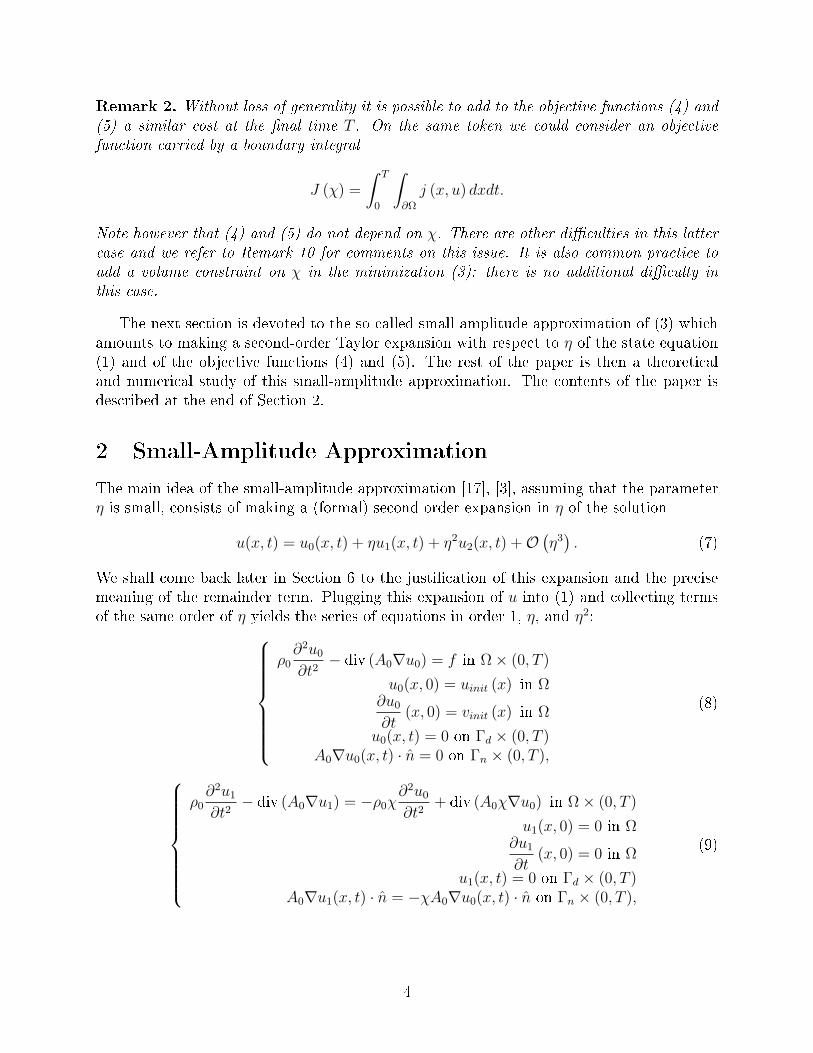
[4]), for which the state equation is of Helmholtz type, i.e. the wave equation in the frequencydomain. Very few papers are concerned with a time dependent state equation, be it the heatequation [16] or the wave equation (in the time domain) [11], [13], [15]. One possible reasonfor this lack of contributions is the additional diculties which arise in this context. From atheoretical point of view, we see at least two of them. First, there are no simple situations,like single state equations in the conductivity setting or compliance minimization in theelasticity setting, where the optimality condition helps in reducing the complexity of theoptimal microstructure. For example, optimal microstructures are unknown for any typeof objective function in the elastodynamics setting. Second, the relaxation of a gradient-based objective function relies on a corrector result which is not available for the waveequation except for well-prepared initial data [6]. Of course, these theoretical dicultieshave numerical counterparts and, even when the relaxed formulation is available, the optimalmicrostructures are complicated, typically laminates of high rank. Therefore there is room fora simplied setting, allowing for a complete theoretical and numerical treatment. Followingthe lead of [3] we suggest to consider a second order small-amplitude approximation of theproblem and to relax it by using the theory of H-measures, due to Gérard [8] and Tartar [17].The use of H-measures for studying small-amplitude composite materials was previouslyinitiated by Tartar [17]: the main advantage is the induced simplication in the analysissince the necessary tools of homogenization theory are replaced by the simpler notion ofH-measures (see Remark 13 below).
Let us present our model problem which, for simplicity, is expressed for a scalar-valuedunknown, like in a conductivity model. We hasten to say that all our results are also validin the elasticity setting or in any other multiphysics or multiple loads setting (see Remark16). In particular, all our numerical computations will be made for the linearized elasticitysystem. We consider a smooth bounded open set Ω in RN lled by two isotropic materialsof nearly equal conductivity or elasticity tensors. Specically we consider a region withcharacteristic function χ to contain a material with conductivity (or elasticity) tensor A1,the complementary region in Ω contains a second material of conductivity (or elasticity)tensor A0. The two tensors are assumed to be symmetric, coercive and related by thecontrast parameter η,
A1 = (1 + η)A0,
yielding the overall tensor
Aχ(x) = A0 (1− χ(x)) + A1χ(x) = A0 (1 + ηχ(x)) .
We assume the same contrast relation for the positive material densities, i.e., ρ1 = (1 + η) ρ0
andρχ(x) = ρ0 (1− χ(x)) + ρ1χ(x) = ρ0 (1 + ηχ(x)) .
For a given nal time 0 < T < +∞, we consider waves propagating in the domain Ω. In
2

other words, we look at the wave equation:
ρ0 (1 + ηχ)∂2u
∂t2− div (A0 (1 + ηχ)∇u) = f in Ω× (0, T )
u(x, 0) = uinit (x) in Ω∂u
∂t(x, 0) = vinit (x) in Ω
u(x, t) = 0 on Γd × (0, T )A0 (1 + ηχ)∇u(x, t) · n = 0 on Γn × (0, T ),
(1)
where Γd,Γn is a smooth partition of the boundary ∂Ω (with Γd of positive (N − 1)-dimensional measure). Introducing the function space V , dened by
V = φ ∈ H1(Ω) such that φ = 0 on Γd, (2)
we assume that uinit ∈ V and vinit ∈ L2 (Ω) are initial data and f ∈ L2 ((0, T )× Ω) isan applied force. As is well-known there exists a unique solution u of (1) in the spaceC0 ([0, T ];V )∩C1 ([0, T ];L2(Ω)). Actually we shall assume that the initial data are smootherfor an additional regularity of solutions (see Lemma 1 and Remark 12 for details and com-ments).
Remark 1. There is no conceptual diculty in replacing the homogeneous boundary datain (1) by non homogeneous Dirichlet and/or Neumann ones, having sucient smoothness.For the sake of clarity in the exposition we do not treat the case of inhomogeneous boundarydata.
An optimal design problem associated to the wave equation (1) is the minimization of anobjective function
infχ∈L∞(Ω;0,1)
J (χ) (3)
where J(χ) depends implicitly on χ through the solution u. Two typical examples of objectivefunction are
J (χ) =
∫ T
0
∫Ω
j (x, u) dxdt, (4)
and
J (χ) =
∫ T
0
∫Ω
j (x,∇u) dxdt. (5)
In both cases we assume that the integrand j(x, λ) is a Carathéodory function, of class C2
with adequate growth conditions with respect to its second argument. Typically, we assumethat there exists a constant C > 0 such that, for any x ∈ Ω and λ ∈ R (or λ ∈ RN),
|j(x, λ)| ≤ C(|λ|2 + 1), |j′(x, λ)| ≤ C(|λ|+ 1), |j′′(x, λ)| ≤ C, (6)
where the notation ′ means derivation with respect to the second argument λ. Of course,more subtle and less restrictive assumptions are possible. In the sequel, for the ease ofnotations we shall drop the dependence on x in the denition of j(x, λ).
3
Remark 2. Without loss of generality it is possible to add to the objective functions (4) and(5) a similar cost at the nal time T . On the same token we could consider an objectivefunction carried by a boundary integral
J (χ) =
∫ T
0
∫∂Ω
j (x, u) dxdt.
Note however that (4) and (5) do not depend on χ. There are other diculties in this lattercase and we refer to Remark 10 for comments on this issue. It is also common practice toadd a volume constraint on χ in the minimization (3): there is no additional diculty inthis case.
The next section is devoted to the so-called small-amplitude approximation of (3) whichamounts to making a second-order Taylor expansion with respect to η of the state equation(1) and of the objective functions (4) and (5). The rest of the paper is then a theoreticaland numerical study of this small-amplitude approximation. The contents of the paper isdescribed at the end of Section 2.
2 Small-Amplitude Approximation
The main idea of the small-amplitude approximation [17], [3], assuming that the parameterη is small, consists of making a (formal) second order expansion in η of the solution
u(x, t) = u0(x, t) + ηu1(x, t) + η2u2(x, t) +O(η3). (7)
We shall come back later in Section 6 to the justication of this expansion and the precisemeaning of the remainder term. Plugging this expansion of u into (1) and collecting termsof the same order of η yields the series of equations in order 1, η, and η2:
ρ0∂2u0
∂t2− div (A0∇u0) = f in Ω× (0, T )
u0(x, 0) = uinit (x) in Ω∂u0
∂t(x, 0) = vinit (x) in Ω
u0(x, t) = 0 on Γd × (0, T )A0∇u0(x, t) · n = 0 on Γn × (0, T ),
(8)
ρ0∂2u1
∂t2− div (A0∇u1) = −ρ0χ
∂2u0
∂t2+ div (A0χ∇u0) in Ω× (0, T )
u1(x, 0) = 0 in Ω∂u1
∂t(x, 0) = 0 in Ω
u1(x, t) = 0 on Γd × (0, T )A0∇u1(x, t) · n = −χA0∇u0(x, t) · n on Γn × (0, T ),
(9)
4

ρ0∂2u2
∂t2− div (A0∇u2) = −ρ0χ
∂2u1
∂t2+ div (A0χ∇u1) in Ω× (0, T )
u2(x, 0) = 0 in Ω∂u2
∂t(x, 0) = 0 in Ω
u2(x, t) = 0 on Γd × (0, T )A0∇u2(x, t) · n = −χA0∇u1(x, t) · n on Γn × (0, T ).
(10)
Obviously (8) contains no dependency upon the characteristic function χ and it admits aunique solution u0 in the space C0 ([0, T ];V )∩C1 ([0, T ];L2(Ω)). However problems (9) and(10) do depend upon χ and, since their right hand sides are not smooth a priori, existenceof the solutions u1 and u2 needs to be established. We postpone this matter for the momentand refer to Lemma 3 below.
We then plug the ansatz (7) into the objective function J(χ) which we want to minimize.We dene the small-amplitude objective function Jsa(χ) as its second order truncation,namely
J (χ) = Jsa (χ) +O(η3),
where, for the objective function (4), we have
Jsa (χ) =
∫ T
0
∫Ω
(j (u0) + ηj′ (u0)u1 + η2
(j′ (u0)u2 +
1
2j′′ (u0) (u1)2
))dxdt, (11)
while, for the other objective function (5), we obtain instead
Jsa (χ) =
∫ T
0
∫Ω
(j(∇u0)+ηj′(∇u0)·∇u1+η2
(j′(∇u0) · ∇u2 +
1
2j′′(∇u0)∇u1 · ∇u1
))dxdt.
(12)Again we have to prove that formula (11) or (12) makes sense for the solutions u0, u1, u2 of(8), (9) and (10) (see Lemma 3 below). Note that we have dropped the dependence on x forthe integrand j and its derivative for the sake of simplicity in the presentation.
We call the following minimization the small-amplitude optimization problem,
infχ∈L∞(Ω;0,1)
Jsa (χ) . (13)
Here Jsa is dened by (11) or (12). Although (13) is a simplied approximation of (3) itis still not a well-posed problem, namely it does not admit minimizer. Indeed, minimizingsequences of (13) do not usually converge to another characteristic function, taking onlyvalues 0 and 1 on Ω, but rather converge (weakly) to a density, taking values in the entireinterval [0, 1]. It is thus necessary to relax the small amplitude problem (13). In the caseof elliptic PDE's, this relaxation has already been carried out in [3] using the theory of H-measures. Section 4 is precisely devoted to a short presentation of this necessary tool whichis simpler than the full theory of homogenization. Before this Section 3 is devoted to variousnecessary a priori estimates which, in particular, will justify the existence of u1 and u2, aswell as the fact that the small-amplitude objective function Jsa is well dened. Section 5 willthen be devoted to the relaxation of the small-amplitude optimization problem (13). Thejustication that (13) is an approximation of the original problem (3) at order O (η3) is the
5
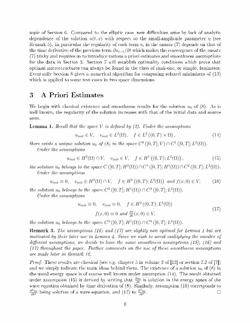
topic of Section 6. Compared to the elliptic case, new diculties arise by lack of analyticdependence of the solution u(t, x) with respect to the small-amplitude parameter η (seeRemark 5). In particular the regularity of each term ui in the ansatz (7) depends on that ofthe time derivative of the previous term ∂ui−1/∂t which makes the convergence of the ansatz(7) tricky and requires us to introduce various a priori estimates and smoothness assumptionsfor the data in Section 3. Section 7 will establish optimality conditions which prove thatoptimal microstructures can always be found in the class of rank-one, or simple, laminates.Eventually Section 8 gives a numerical algorithm for computing relaxed minimizers of (13)which is applied to some test cases in two space dimensions.
3 A Priori Estimates
We begin with classical existence and smoothness results for the solution u0 of (8). As iswell known, the regularity of the solution increases with that of the initial data and sourceterm.
Lemma 1. Recall that the space V is dened by (2). Under the assumptions
uinit ∈ V, vinit ∈ L2(Ω), f ∈ L2 ((0, T )× Ω) , (14)
there exists a unique solution u0 of (8) in the space C0 ([0, T ];V ) ∩ C1 ([0, T ];L2(Ω)).Under the assumptions
uinit ∈ H2(Ω) ∩ V, vinit ∈ V, f ∈ H1((0, T );L2(Ω)
), (15)
the solution u0 belongs to the space C ([0, T ];H2(Ω))∩C1 ([0, T ];H1(Ω))∩C2 ([0, T ];L2(Ω)).Under the assumptions
uinit ≡ 0, vinit ∈ H2(Ω) ∩ V, f ∈ H2((0, T );L2(Ω)
)and f(x, 0) ∈ V, (16)
the solution u0 belongs to the space C2 ([0, T ];H1(Ω)) ∩ C3 ([0, T ];L2(Ω)).Under the assumptions
uinit ≡ 0, vinit ≡ 0, f ∈ H3 ((0, T );L2(Ω))
f(x, 0) ≡ 0 and ∂f∂t
(x, 0) ∈ V,(17)
the solution u0 belongs to the space C3 ([0, T ];H1(Ω)) ∩ C4 ([0, T ];L2(Ω)).
Remark 3. The assumptions (16) and (17) are slightly non optimal for Lemma 1 but aremotivated by their later use in Lemma 4. Since we wish to avoid multiplying the number ofdierent assumptions, we decide to have the same smoothness assumptions (15), (16) and(17) throughout the paper. Further comments on the use of these smoothness assumptionsare made later in Remark 12.
Proof. These results are classical (see e.g. chapter 5 in volume 2 of [12] or section 7.2 of [7])and we simply indicate the main ideas behind them. The existence of a solution u0 of (8) inthe usual energy space is of course well known under assumption (14). The result obtainedunder assumption (15) is derived by writing that ∂u0
∂tis solution in the energy space of the
wave equation obtained by time derivation of (8). Similarly, assumption (16) corresponds to∂2u0
∂t2being solution of a wave equation, and (17) to ∂3u0
∂t3.
6
The next step is to prove a priori estimates for u1 and u2 that will be uniform withrespect to the characteristic function χ. To this end, we prove a lemma on a priori estimatesfor the solution of a generic wave equation, similar to (9) and (10), with an integer i ≥ 1,
ρ0∂2ui∂t2− div (A0∇ui) = −ρ0χ
∂2ui−1
∂t2+ div (A0χ∇ui−1) in Ω× (0, T )
ui(x, 0) = 0 in Ω∂ui∂t
(x, 0) = 0 in Ω
ui(x, t) = 0 on Γd × (0, T )A0∇ui(x, t) · n = −χA0∇ui−1(x, t) · n on Γn × (0, T ).
(18)
We introduce the energy space ET dened by
ET = ϕ such that∂ϕ
∂t∈ L∞
((0, T );L2(Ω)
), and ∇ϕ ∈ L∞
((0, T );L2(Ω)N
)
with the norm
‖φ‖ET=
∥∥∥∥∂φ∂t∥∥∥∥L∞((0,T );L2(Ω))
+ ‖∇φ‖L∞((0,T );L2(Ω)N ).
Lemma 2. If ui−1 belongs to ET , then there exists a unique solution ui of (18) in the spaceC0 ([0, T ];L2(Ω))∩C1 ([0, T ];V ′) where V ′ is the dual space of V dened in (2). Furthermore,there exists a constant C(T ), which does not depend on the characteristic function χ, suchthat the solution of (18) satises
‖ui‖L∞((0,T );L2(Ω)) ≤ C(T )‖ui−1‖ET. (19)
If furthermore ∂ui−1/∂t belongs to ET , then there exists a unique solution ui of (18) inthe space C0 ([0, T ];V )∩C1 ([0, T ];L2(Ω)) and there exists a constant C(T ), which does notdepend on the characteristic function χ, such that the solution of (18) satises
‖ui‖ET≤ C(T )
(‖ui−1‖ET
+ ‖∂ui−1
∂t‖ET
). (20)
Proof. The existence of solutions to (18) in the proposed spaces is classical [7], [12]. Multi-plying equation (18) by ∂ui/∂t and integrating by parts yields the usual energy equality
1
2
d
dt
∫Ω
(ρ0
∣∣∣∣∂ui∂t∣∣∣∣2 + A0∇ui · ∇ui
)dx =
∫Ω
(−ρ0χ
∂2ui−1
∂t2∂ui∂t− A0χ∇ui−1 · ∇
∂ui∂t
)dx.
Integrating by parts in time the last term in the above equality leads to
−∫ T
0
∫Ω
A0χ∇ui−1 ·∇∂ui∂tdtdx =
∫ T
0
∫Ω
A0χ∇∂ui−1
∂t·∇uidtdx−
∫Ω
A0χ∇ui−1(T )·∇ui(T )dx.
By standard arguments, and using the smoothness of ui−1, we deduce from this energyequality the estimate (20) in the energy space ET .
7
If ui−1 is less smooth, namely merely belonging to ET , we need to introduce a timeregularization, dened by
vi (x, t) =
∫ t
0
ui(x, s) ds .
The equation satised by vi is
ρ0∂2vi∂t2− div (A0∇vi) = −ρ0χ
∂ui−1
∂t+ div (A0χ∇vi−1) in Ω× (0, T )
vi(x, 0) = 0 in Ω∂vi∂t
(x, 0) = 0 in Ω
vi(x, t) = 0 on Γd × (0, T )A0∇vi(x, t) · n = −A0∇vi−1(x, t) · n on Γn × (0, T ).
(21)
The energy estimate for (21) is obtained by multiplying it by ∂vi
∂t
1
2
d
dt
∫Ω
(ρ0
∣∣∣∣∂vi∂t∣∣∣∣2 + A0∇vi · ∇vi
)dx =
∫Ω
(−ρ0χ
∂ui−1
∂t
∂vi∂t− A0χ∇vi−1 · ∇
∂vi∂t
)dx.
The rst term in the right hand side causes no problem since −ρ0χ∂ui−1
∂tis bounded in
L∞ ((0, T );L2(Ω)). For the second one we perform a time integration by parts to get
−∫ T
0
∫Ω
A0χ∇vi−1 · ∇∂vi∂tdtdx =
∫ T
0
∫Ω
A0χ∇ui−1 · ∇vidtdx−∫
Ω
A0χ∇vi−1(T ) · ∇vi(T )dx
which can easily be bounded since ui−1 belongs to ET . Therefore we deduce estimate (19).
As a consequence of Lemma 2 we obtain the following justication of all terms involvedin our small amplitude problem.
Lemma 3. Under the assumptions (15) for the data, the solution u1 of (9) belongs to theenergy space ET and the solution u2 of (10) belongs to L∞ ((0, T );L2(Ω)). Eventually, thesmall amplitude objective function (11) is well dened and has nite value. The same is truefor the other objective function (12) if we add a condition on the integrand j on the boundaryΓn, namely
j′(x, λ) = g(x, λ)A0λ ∀x ∈ Γn, λ ∈ RN , (22)
for some real valued function g(x, λ).
Proof. By our assumptions on the data, Lemma 1 implies that the solution u0 of (8) issuch that ∂u0
∂t∈ ET . Applying estimate (20) of Lemma 2 implies that u1 belongs to ET .
Subsequently, estimate (19) of Lemma 2 yields that u2 belongs to L∞ ((0, T );L2(Ω)). Inview of assumption (6) it implies that the small amplitude objective function (11) is a niteintegral. Concerning the gradient-based objective function (12), the only dicult term is∫ T
0
∫Ω
η2j′(∇u0) · ∇u2dxdt
8
because ∇u2 does not belong to L∞ ((0, T );L2(Ω)N
). However, since u0 ∈ C ([0, T ];H2(Ω)),
then j′(∇u0) belongs to C ([0, T ];H1(Ω)) and the above integral makes sense by an integra-tion by parts ∫ T
0
∫Ω
η2j′(∇u0) · ∇u2dxdt = −∫ T
0
∫Ω
η2div (j′(∇u0))u2dxdt (23)
because of the boundary conditions for u0, u2 and (22). Therefore (12) is well dened andnite.
Remark 4. One can avoid the technical assumption (22) for the gradient-based objectivefunction in Lemma 3 if we replace the smoothness assumptions (15) for the data by (16).Then, the result (28) in Lemma 4 implies directly that ∇u2 belongs to L
∞ ((0, T );L2(Ω)) andthere is no need to perform the integration by parts (23).
Remark 5. Lemma 2 suggests a lack of analyticity for the solution u of the wave equation(1) with respect to the parameter η, at least in the energy space ET . Indeed, writing u as aseries in η,
u(x, t) =∑i≥0
ηiui(x, t),
estimate (20) indicates that each term ui can be controled in ET merely by ∂ui−1
∂t, so no
convergence in ET can be expected. Let us point out that, even if (20) is not optimal (forexample, the upper bound can be evaluated in the L1-norm in time), one cannot avoid to"lose" one derivative in the norm of ui−1 controlling that of ui. This is in sharp contrastwith the elliptic case, where the solution depends analytically on the parameter η [17], andexplains the additional diculties in the sequel.
As a convincing example, we now show that this lack of analyticity is obvious, for anyreasonable Sobolev-type norm, on the explicit solution for a one-dimensional wave equationwith constant coecients on the entire line R without any source term. Indeed, in such acase the explicit solution is given as the superposition of two waves travelling in oppositedirections
u(x, t) = a+(x− ct) + a−(x+ ct)
where the functions a± are determined by the initial data and c =√A/ρ is the sound speed.
Clearly, the derivatives of u with respect to the parameter c involves derivatives of a±, whichare equivalent to time derivatives of u. Thus one cannot obtain a convergent Taylor seriesof u with respect to c if u merely belongs to a functional space involving a nite number ofderivatives (as the energy space) and is not at least ininitely dierentiable with respect to(x, t).
For the reasons detailed in Remark 5 we shall need further smoothness of the solutionof (18), beyond that provided by Lemma 2. A remarkable feature of the boundary valueproblem (18) is that the time derivative of its solution wi = ∂ui/∂t satises a system of thesame type, except with dierent initial data. This is of course a consequence of the fact thatthe characteristic function χ does not depend on time t. More precisely, for i ≥ 1, wi = ∂ui
∂t
9

is formally a solution of
ρ0∂2wi∂t2− div (A0∇wi) = −ρ0χ
∂2wi−1
∂t2+ div (A0χ∇wi−1) in Ω× (0, T )
wi(x, 0) = 0 in Ω
∂wi∂t
(x, 0) =∂2ui∂t2
(x, 0) in Ω
wi(x, t) = 0 on Γd × (0, T )A0∇wi(x, t) · n = −χA0∇wi−1(x, t) · n on Γn × (0, T ),
(24)
with the initial velocity
∂wi∂t
(x, 0) =∂2ui∂t2
(x, 0) = −χ∂2ui−1
∂t2+
1
ρ0
(div (A0∇ui) + div (A0χ∇ui−1)) . (25)
Similarly, the second-order time derivative zi = ∂2ui
∂t2formally satisifes
ρ0∂2zi∂t2− div (A0∇zi) = −ρ0χ
∂2zi−1
∂t2+ div (A0χ∇zi−1) in Ω× (0, T )
zi(x, 0) =∂2ui∂t2
(x, 0) in Ω
∂zi∂t
(x, 0) =∂2wi∂t2
(x, 0) in Ω
zi(x, t) = 0 on Γd × (0, T )A0∇zi(x, t) · n = −χA0∇zi−1(x, t) · n on Γn × (0, T )
(26)
with initial position given by (25) and initial velocity
∂zi∂t
(x, 0) =∂2wi∂t2
(x, 0) = −χ∂2wi−1
∂t2+
1
ρ0
(div (A0∇wi) + div (A0χ∇wi−1)) . (27)
Fortunately, in the sequel we need only a priori estimates for w1 and z1, which thus dependson the smoothness of u0. We therefore require additional smoothness of the data.
Lemma 4. Under the assumptions (16) for the data, we have
‖w1‖ET≤ C(T ) where w1 =
∂u1
∂t. (28)
Under the assumptions (17) for the data, we have
‖z1‖ET≤ C(T ) where z1 =
∂2u1
∂t2. (29)
In both (28) and (29) the constant C(T ) does not depend on the characteristic function χ.
Proof. We rst prove (28). By Lemma 1 the assumptions (16) imply that ∂w0
∂t= ∂2u0
∂t2∈ ET
so the source term in (24), for i = 1, belongs to the dual of ET and causes no problem. The
10

main diculty is to evaluate the smoothness of the initial velocity (25). Using equation (9),and since u1(x, 0) = 0, we compute
∂w1
∂t(x, 0) =
1
ρ0
(− χf(x, 0) + A0∇χ · ∇uinit(x)
). (30)
To obtain that w1 belongs to the energy space ET we must have ∂w1
∂t(x, 0) ∈ L2(Ω) and since
χ is discontinuous and unknown, the only possibility is to assume that uinit vanishes. Thisnishes the proof of (28).
We then prove (29). The source term in (26), for i = 1, belongs to the dual of ET if∂z0∂t
= ∂3u0
∂t3∈ ET . This is the case in view of Lemma 1 and our assumptions (17). The initial
position z1(x, 0) = ∂w1
∂t(x, 0) has already been computed in (30): it further belongs to H1(Ω)
if f(x, 0) ≡ 0 because χ is discontinuous. The initial velocity is computed through equation(24) for i = 1:
∂z1
∂t(x, 0) =
∂2w1
∂t2(x, 0) =
1
ρ0
(div (A0∇w1)− ρ0χ
∂2w0
∂t2+ div (A0χ∇w0)
)(x, 0) .
Since w1(x, 0) = 0 and using the time derivative of equation (8) we deduce
∂z1
∂t(x, 0) =
1
ρ0
(− χ∂f
∂t(x, 0) + A0∇χ · ∇vinit(x)
). (31)
To obtain that z1 belongs to the energy space ET we must have ∂z1∂t
(x, 0) ∈ L2(Ω) and sinceχ is discontinuous and unknown, the only possibility is to assume that vinit vanishes. Thisnishes the proof of (29).
4 A brief review of H-measure theory
We briey recall the denition of H-measures, introduced by Gérard [8] and Tartar [17].An H-measure is a default measure which quanties the lack of compactness of weaklyconverging sequences in L2(RN). More precisely, it indicates where in the physical space,and at which frequency in the Fourier space, are the obstructions to strong convergence.Since their inception H-measures have been the right tool for studying small amplitudehomogenization [17] and related optimal design problems [3]. All results below are due to[8] and [17], to which we refer for complete proofs.
We denote by SN−1 the unit sphere in RN , C(SN−1) is the space of continuous complex-valued functions on SN−1, and C0(RN) is that of continuous complex-valued functions de-creasing to 0 at innity in RN . As usual z denotes the complex conjugate of the complexnumber z. The Fourier transform operator in L2(RN), denoted by F , is dened by
(Fφ) (ξ) =
∫RN
φ(x)e−2iπx·ξdx ∀φ ∈ L2(RN).
Theorem 1. Let uε = (uiε)1≤i≤p be a sequence of functions dened in RN with values in Rp
which converges weakly to 0 in L2(RN)p. There exists a subsequence (still denoted by ε) and
11
a family of complex-valued Radon measures (µij(x, ξ))1≤i,j≤p on RN × SN−1 such that, forany functions φ1(x), φ2(x) ∈ C0(RN) and ψ(ξ) ∈ C(SN−1), it satises
limε→0
∫RN
F(φ1u
iε
)(ξ)F
(φ2u
jε
)(ξ)ψ
(ξ
|ξ|
)dξ =
∫RN
∫SN−1
φ1(x)φ2(x)ψ(ξ)µij(dx, dξ) .
The matrix of measures µ = (µij)1≤i,j≤p is called the H-measure of the subsequence uε. It ishermitian and non-negative, i.e.
µij = µji,
p∑i,j=1
λiλjµij ≥ 0 ∀λ ∈ Cp.
If we consider a sequence uε which converges weakly in L2(RN)p to a limit u (insteadof 0), then, applying Theorem 1 to (uε − u), and taking ψ ≡ 1, we obtain a representationformula for the limit of quadratic expressions of uε
limε→0
∫RN
φ1φ2uiεu
jε dx =
∫RN
φ1φ2uiuj dx+
∫RN
∫SN−1
φ1(x)φ2(x)µij(dx, dξ) . (32)
Therefore the H-measure appears as a default measure which gives a precise representationof the compactness default, taking into account the directions of the oscillation.
If some information is known on the derivatives of the sequence uε, then more can besaid on the H-measure: this is a localization principle for the support of the H-measure.
Theorem 2. Let uε = (uiε)1≤i≤p be a sequence of functions dened in RN with values in Rp
which converges weakly to 0 in L2(RN)p and denes an H-measure µ(x, ξ) = (µij(x, ξ))1≤i,j≤p.If, furthermore, uε satises the constraint
p∑j=1
N∑k=1
∂
∂xk
(Cjk(x)ujε
)→ 0 in H−1
loc (Ω) strongly,
where the coecients Cjk(x) are continuous functions in Ω ⊂ RN , then
p∑j=1
N∑k=1
ξkCjk(x)µjm(x, ξ) = 0 in Ω× SN−1, for any 1 ≤ m ≤ p.
We now recall the particular case of characteristic functions [10], [17].
Lemma 5. Let χε(x) be a sequence of characteristic functions that weakly-* converges to alimit θ(x) in L∞(Ω; [0, 1]). Then the corresponding H-measure µ for the sequence (χε − θ)is necessarily of the type
µ(dx, dξ) = θ(x)(
1− θ(x))ν(dx, dξ)
where, for given x, the measure ν(dx, dξ) is a probability measure with respect to ξ, i.e.ν ∈ P(Ω,SN−1) with
P(Ω,SN−1) =
ν(x, ξ) Radon measure on Ω× SN−1 such that:
ν ≥ 0,
∫SN−1
ν(x, ξ) dξ = 1 a.e. x ∈ Ω
. (33)
12

Conversely, for any such probability measure ν ∈ P(Ω,SN−1) there exists a sequence χε,which weakly-* converges to θ in L∞(Ω; [0, 1]), such that θ(1 − θ)ν is the H-measure of(χε − θ).
Remark 6. In the periodic setting the notion of H-measure has a very simple interpretationand it is often called two-point correlation function in the context of composite materials[14]. Indeed, let u(x, y) be a smooth function dened on Ω × Y , with Y = (0, 1)N , suchthat y → u(x, y) is Y -periodic. Assuming that
∫Yu(x, y)dy = 0, it is easily seen that
uε(x) = u(x, x/ε) converges weakly to 0 in L2(Ω). By using the Fourier series decompositionin Y , the H-measure µ of uε is simple to compute. Introducing
u(x, y) =∑k∈ZN
u(x, k)e2iπk·y,
we deduce
µ(x, ξ) =∑
k 6=0∈ZN
|u(x, k)|2δ(ξ − k
|k|
),
where δ is the Dirac mass.
5 Relaxed Formulation
The optimization problem (13) is not well-posed in the sense that it usually does not admit aminimizer. Indeed, a minimizing sequence of characteristic functions χε does not necessarilyconverge to a characteristic function χ0, but rather to some limit density θ. In this sectionwe give the relaxed formulation of (13) using the theory of H-measures. In other wordswe compute the limit, as ε goes to 0, of the state equations (9), (10) and of the objectivefunctions (11), (12), evaluated for the characteristic function χε.
We shall pass to the limit rst in the state equations, which requires little smoothness ofthe data, and second in the objective functions, which is more demanding on the regularityof the data. We begin with a lemma on a priori estimates for the solutions of (9) and (10).
Lemma 6. For any sequence of characteristic functions χε we denote by uε1 and uε2 therespective solutions of (9) and (10). Under the assumptions (15) for the data, there exists aconstant C(T ), which does not depend on ε, such that
‖uε1‖ET≤ C(T ), (34)
and‖uε2‖L∞((0,T );L2(Ω)) ≤ C(T ). (35)
Proof. The present lemma is just a combination of Lemmas 3 and 2. In particular, estimates(34) and (35) are simple consequences of Lemma 2.
Lemma 7. Assume that the data satisfy the smoothness assumption (15). For any sequenceof characteristic functions χε there exist a subsequence and limits θ ∈ L∞ (Ω; [0, 1]) andν ∈ P(Ω,SN−1), dened by (33), such that:
χε θ weakly * in L∞ (Ω; [0, 1]) and θ(1− θ)ν is the H-measure of (χε − θ) .
13
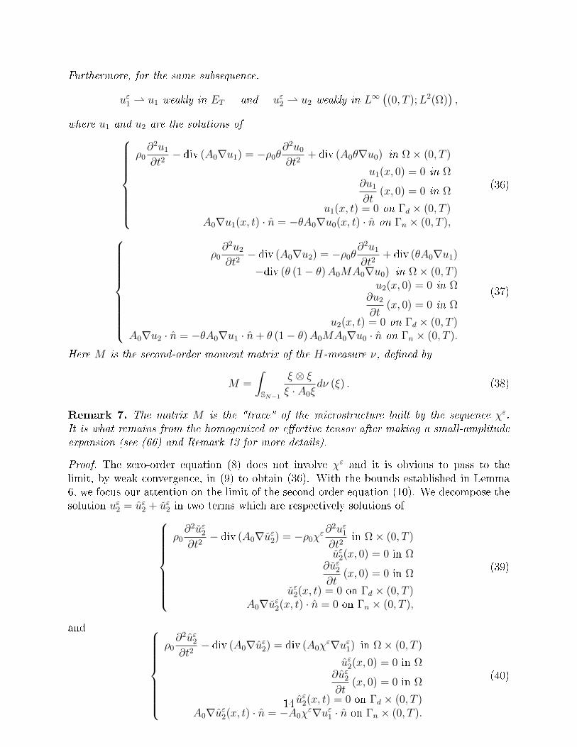
Furthermore, for the same subsequence,
uε1 u1 weakly in ET and uε2 u2 weakly in L∞((0, T );L2(Ω)
),
where u1 and u2 are the solutions of
ρ0∂2u1
∂t2− div (A0∇u1) = −ρ0θ
∂2u0
∂t2+ div (A0θ∇u0) in Ω× (0, T )
u1(x, 0) = 0 in Ω∂u1
∂t(x, 0) = 0 in Ω
u1(x, t) = 0 on Γd × (0, T )A0∇u1(x, t) · n = −θA0∇u0(x, t) · n on Γn × (0, T ),
(36)
ρ0∂2u2
∂t2− div (A0∇u2) = −ρ0θ
∂2u1
∂t2+ div (θA0∇u1)
−div (θ (1− θ)A0MA0∇u0) in Ω× (0, T )u2(x, 0) = 0 in Ω
∂u2
∂t(x, 0) = 0 in Ω
u2(x, t) = 0 on Γd × (0, T )A0∇u2 · n = −θA0∇u1 · n+ θ (1− θ)A0MA0∇u0 · n on Γn × (0, T ).
(37)
Here M is the second-order moment matrix of the H-measure ν, dened by
M =
∫SN−1
ξ ⊗ ξξ · A0ξ
dν (ξ) . (38)
Remark 7. The matrix M is the "trace" of the microstructure built by the sequence χε.It is what remains from the homogenized or eective tensor after making a small-amplitudeexpansion (see (66) and Remark 13 for more details).
Proof. The zero-order equation (8) does not involve χε and it is obvious to pass to thelimit, by weak convergence, in (9) to obtain (36). With the bounds established in Lemma6, we focus our attention on the limit of the second-order equation (10). We decompose thesolution uε2 = uε2 + uε2 in two terms which are respectively solutions of
ρ0∂2uε2∂t2− div (A0∇uε2) = −ρ0χ
ε∂2uε1∂t2
in Ω× (0, T )
uε2(x, 0) = 0 in Ω∂uε2∂t
(x, 0) = 0 in Ω
uε2(x, t) = 0 on Γd × (0, T )A0∇uε2(x, t) · n = 0 on Γn × (0, T ),
(39)
and
ρ0∂2uε2∂t2− div (A0∇uε2) = div (A0χ
ε∇uε1) in Ω× (0, T )
uε2(x, 0) = 0 in Ω∂uε2∂t
(x, 0) = 0 in Ω
uε2(x, t) = 0 on Γd × (0, T )A0∇uε2(x, t) · n = −A0χ
ε∇uε1 · n on Γn × (0, T ).
(40)
14
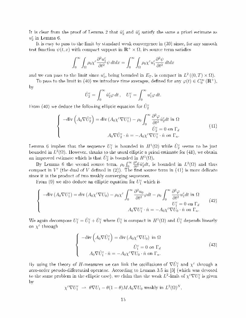
It is clear from the proof of Lemma 2 that uε2 and uε2 satisfy the same a priori estimate asuε2 in Lemma 6.
It is easy to pass to the limit by standard weak convergence in (39) since, for any smoothtest function ψ(t, x) with compact support in R+ × Ω, its source term satises∫ ∞
0
∫Ω
ρ0χε∂
2uε1∂t2
ψ dtdx =
∫ ∞0
∫Ω
ρ0χεuε1
∂2ψ
∂t2dtdx
and we can pass to the limit since uε1, being bounded in ET , is compact in L2 ((0, T )× Ω).To pass to the limit in (40) we introduce time averages, dened for any ϕ(t) ∈ C∞0 (R+),
by
U ε2 =
∫ ∞0
uε2ϕdt , U ε1 =
∫ ∞0
uε1ϕdt.
From (40) we deduce the following elliptic equation for U ε2
−div(A0∇U ε
2
)= div (A0χ
ε∇U ε1 )− ρ0
∫ ∞0
∂2ϕ
∂t2uε2dt in Ω
U ε2 = 0 on Γd
A0∇U ε2 · n = −A0χ
ε∇U ε1 · n on Γn.
(41)
Lemma 6 implies that the sequence U ε1 is bounded in H1(Ω) while U ε
2 seems to be justbounded in L2(Ω). However, thanks to the usual elliptic a priori estimate for (41), we obtainan improved estimate which is that U ε
2 is bounded in H1(Ω).
By Lemma 6 the second source term, ρ0
∫∞0
∂2ϕ∂t2uε2dt, is bounded in L2(Ω) and thus
compact in V ′ (the dual of V dened in (2)). The rst source term in (41) is more delicatesince it is the product of two weakly converging sequences.
From (9) we also deduce an elliptic equation for U ε1 which is
−div (A0∇U ε1 ) = div (A0χ
ε∇U0)− ρ0χε
∫ ∞0
∂2u0
∂t2ϕdt− ρ0
∫ ∞0
∂2ϕ
∂t2uε1dt in Ω
U ε1 = 0 on Γd
A0∇U ε1 · n = −A0χ
ε∇U0 · n on Γn.
(42)
We again decompose U ε1 = U ε
1 + U ε1 where U ε
1 is compact in H1(Ω) and U ε1 depends linearly
on χε through −div
(A0∇U ε
1
)= div (A0χ
ε∇U0) in Ω
U ε1 = 0 on Γd
A0∇U ε1 · n = −A0χ
ε∇U0 · n on Γn.
(43)
By using the theory of H-measures we can link the oscillations of ∇U ε1 and χε through a
zero-order pseudo-dierential operator. According to Lemma 3.5 in [3] (which was devotedto the same problem in the elliptic case), we claim that the weak L2-limit of χε∇U ε
1 is givenby
χε∇U ε1 θ∇U1 − θ(1− θ)MA0∇U0 weakly in L2(Ω)N ,
15
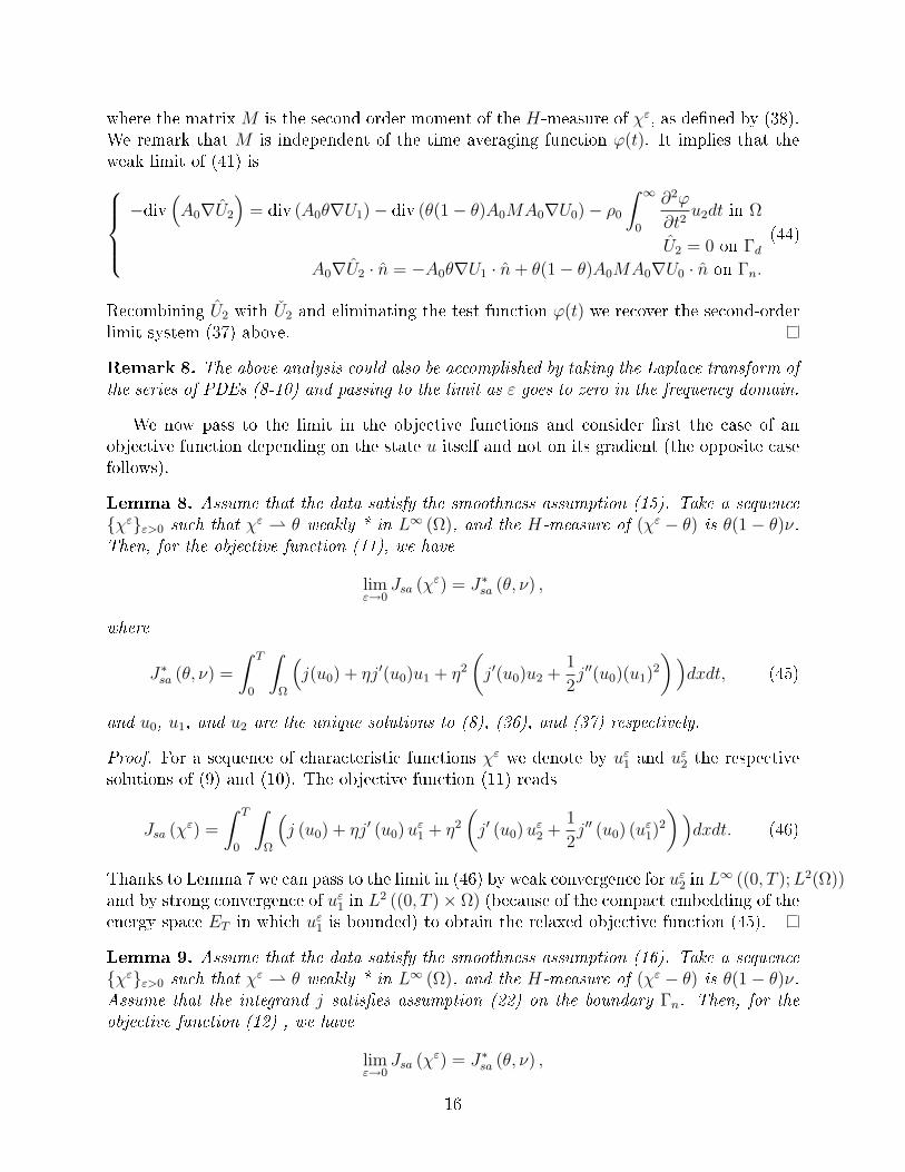
where the matrix M is the second order moment of the H-measure of χε, as dened by (38).We remark that M is independent of the time averaging function ϕ(t). It implies that theweak limit of (41) is−div
(A0∇U2
)= div (A0θ∇U1)− div (θ(1− θ)A0MA0∇U0)− ρ0
∫ ∞0
∂2ϕ
∂t2u2dt in Ω
U2 = 0 on ΓdA0∇U2 · n = −A0θ∇U1 · n+ θ(1− θ)A0MA0∇U0 · n on Γn.
(44)
Recombining U2 with U2 and eliminating the test function ϕ(t) we recover the second-orderlimit system (37) above.
Remark 8. The above analysis could also be accomplished by taking the Laplace transform ofthe series of PDEs (8-10) and passing to the limit as ε goes to zero in the frequency domain.
We now pass to the limit in the objective functions and consider rst the case of anobjective function depending on the state u itself and not on its gradient (the opposite casefollows).
Lemma 8. Assume that the data satisfy the smoothness assumption (15). Take a sequenceχεε>0 such that χε θ weakly * in L∞ (Ω), and the H-measure of (χε − θ) is θ(1 − θ)ν.Then, for the objective function (11), we have
limε→0
Jsa (χε) = J∗sa (θ, ν) ,
where
J∗sa (θ, ν) =
∫ T
0
∫Ω
(j(u0) + ηj′(u0)u1 + η2
(j′(u0)u2 +
1
2j′′(u0)(u1)2
))dxdt, (45)
and u0, u1, and u2 are the unique solutions to (8), (36), and (37) respectively.
Proof. For a sequence of characteristic functions χε we denote by uε1 and uε2 the respectivesolutions of (9) and (10). The objective function (11) reads
Jsa (χε) =
∫ T
0
∫Ω
(j (u0) + ηj′ (u0)uε1 + η2
(j′ (u0)uε2 +
1
2j′′ (u0) (uε1)2
))dxdt. (46)
Thanks to Lemma 7 we can pass to the limit in (46) by weak convergence for uε2 in L∞ ((0, T );L2(Ω))
and by strong convergence of uε1 in L2 ((0, T )× Ω) (because of the compact embedding of the
energy space ET in which uε1 is bounded) to obtain the relaxed objective function (45).
Lemma 9. Assume that the data satisfy the smoothness assumption (16). Take a sequenceχεε>0 such that χε θ weakly * in L∞ (Ω), and the H-measure of (χε − θ) is θ(1 − θ)ν.Assume that the integrand j satises assumption (22) on the boundary Γn. Then, for theobjective function (12) , we have
limε→0
Jsa (χε) = J∗sa (θ, ν) ,
16

where
J∗sa (θ, ν) =
∫ T
0
∫Ω
(j(∇u0) + ηj′(∇u0) · ∇u1 + η2j′(∇u0) · ∇u2
+1
2η2 (j′′(∇u0)∇u1 · ∇u1 + θ(1− θ)A0NA0∇u0 · ∇u0)
)dxdt,
(47)
where N(x) is a matrix dened by
N =
∫SN−1
j′′(∇u0)ξ · ξ(A0ξ · ξ)2
ξ ⊗ ξ dν(ξ) (48)
and u0, u1, and u2 are the unique solutions to (8), (36), and (37) respectively.
Remark 9. The matrix N is the "trace" of the amplication factor in the gradient caused bythe microstructure built by the sequence χε. It is what remains from the notion of correctorin homogenization theory after making a small-amplitude expansion. Recall that correctorsare necessary to get a strong convergence of the solution gradient which otherwise is merelyweak (see [1], [18] if necessary).
Proof. For a sequence of characteristic functions χε, denoting by uε1 and uε2 the respectivesolutions of (9) and (10), the objective function (12) reads
Jsa(χε) =
∫ T
0
∫Ω
(j(∇u0)+ηj′(∇u0)·∇uε1+η2
(j′(∇u0) · ∇uε2 +
1
2j′′(∇u0)∇uε1 · ∇uε1
))dxdt.
(49)To pass to the limit in the third term of (49) we perform an integration by parts, like inLemma 3 under the technical assumption (22),∫ T
0
∫Ω
j′(∇u0) · ∇uε2 dxdt = −∫ T
0
∫Ω
div (j′(∇u0))uε2 dxdt
and we use the weak convergence of uε2 as given by Lemma 7. To pass to the limit in thefourth term of (49) we use again H-measure theory but, contrary to the simple proof ofLemma 7, we need to compute the H-measure of ∇uε1 in terms of that of χε and not merelythe H-measure of a time average of ∇uε1. The argument is thus a little bit more involvedand requires the additional smoothness provided by assumption (16).
We introduce the vector-valued sequence gε(t, x) of the partial derivatives of uε1 plus thecharacteristic function χε
gε =
(∂uε1∂t
,∂uε1∂x1
, · · · , ∂uε1
∂xN, χε)
and for the ease of notations we shall denote the time t by x0. Similarly the Fourier dualvariable of t will be denoted by ξ0. Although gε(t, x) is dened on R+ × Ω we extendit by 0 outside Ω and by solving backward the wave equation (9) for negative time, sowe may consider it as a bounded sequence in L2(RN+1)N+2. In truth, gε is bounded inL∞(R;L2(RN))N+2, but multiplying it by a cut-o function ϕ(t) ∈ C∞c (R) yields the requiredL2 bound and, since (49) is an integral on a nite time interval, this cut-o trick is enough
17
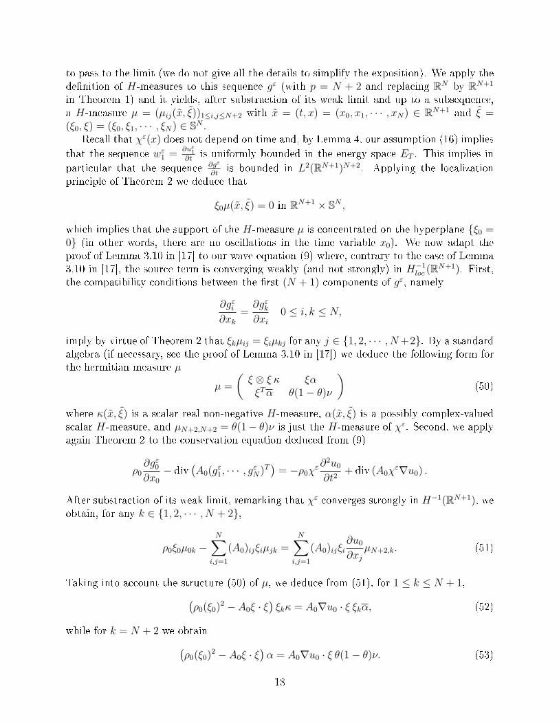
to pass to the limit (we do not give all the details to simplify the exposition). We apply thedenition of H-measures to this sequence gε (with p = N + 2 and replacing RN by RN+1
in Theorem 1) and it yields, after substraction of its weak limit and up to a subsequence,a H-measure µ = (µij(x, ξ))1≤i,j≤N+2 with x = (t, x) = (x0, x1, · · · , xN) ∈ RN+1 and ξ =(ξ0, ξ) = (ξ0, ξ1, · · · , ξN) ∈ SN .
Recall that χε(x) does not depend on time and, by Lemma 4, our assumption (16) implies
that the sequence wε1 =∂uε
1
∂tis uniformly bounded in the energy space ET . This implies in
particular that the sequence ∂gε
∂tis bounded in L2(RN+1)N+2. Applying the localization
principle of Theorem 2 we deduce that
ξ0µ(x, ξ) = 0 in RN+1 × SN ,
which implies that the support of the H-measure µ is concentrated on the hyperplane ξ0 =0 (in other words, there are no oscillations in the time variable x0). We now adapt theproof of Lemma 3.10 in [17] to our wave equation (9) where, contrary to the case of Lemma3.10 in [17], the source term is converging weakly (and not strongly) in H−1
loc (RN+1). First,the compatibility conditions between the rst (N + 1) components of gε, namely
∂gεi∂xk
=∂gεk∂xi
0 ≤ i, k ≤ N,
imply by virtue of Theorem 2 that ξkµij = ξiµkj for any j ∈ 1, 2, · · · , N+2. By a standardalgebra (if necessary, see the proof of Lemma 3.10 in [17]) we deduce the following form forthe hermitian measure µ
µ =
(ξ ⊗ ξ κ ξαξTα θ(1− θ)ν
)(50)
where κ(x, ξ) is a scalar real non-negative H-measure, α(x, ξ) is a possibly complex-valuedscalar H-measure, and µN+2,N+2 = θ(1− θ)ν is just the H-measure of χε. Second, we applyagain Theorem 2 to the conservation equation deduced from (9)
ρ0∂gε0∂x0
− div(A0(gε1, · · · , gεN)T
)= −ρ0χ
ε∂2u0
∂t2+ div (A0χ
ε∇u0) .
After substraction of its weak limit, remarking that χε converges strongly in H−1(RN+1), weobtain, for any k ∈ 1, 2, · · · , N + 2,
ρ0ξ0µ0k −N∑
i,j=1
(A0)ijξiµjk =N∑
i,j=1
(A0)ijξi∂u0
∂xjµN+2,k. (51)
Taking into account the structure (50) of µ, we deduce from (51), for 1 ≤ k ≤ N + 1,(ρ0(ξ0)2 − A0ξ · ξ
)ξkκ = A0∇u0 · ξ ξkα, (52)
while for k = N + 2 we obtain(ρ0(ξ0)2 − A0ξ · ξ
)α = A0∇u0 · ξ θ(1− θ)ν. (53)
18
Since the support of µ, and thus of κ and α, are restricted to the hyperplane ξ0 = 0, wecan simply cancel the term (ξ0)2 in (52) and (53). We also check that α is a real-valuedmeasure and combining (52) and (53) we deduce the following relation between κ and ν
κ(x, ξ) = θ(1− θ)(A0∇u0 · ξA0ξ · ξ
)2
ν(x, ξ)δ(ξ0) (54)
where δ is the usual Dirac mass. From (54) we thus obtain the H-measure of ∇uε1 =(gε1, · · · , gεN)T which is
ξ ⊗ ξκ = θ(1− θ)(A0∇u0 · ξA0ξ · ξ
)2
ξ ⊗ ξ ν(x, ξ)δ(ξ0).
Therefore, the limit of ∫ T
0
∫Ω
j′′(∇u0)∇uε1 · ∇uε1 dxdt
is∫ T
0
∫Ω
j′′(∇u0)∇u1 · ∇u1 dxdt+
∫ T
0
∫Ω
∫SN−1
θ(1− θ)j′′(∇u0)ξ · ξ(A0∇u0 · ξA0ξ · ξ
)2
dν(x, ξ) dt
which is precisely the last line of (47) with formula (48).
Theorem 3. Under the respective assumptions of Lemmas 8 and 9 (depending on our choiceof objective function), the relaxation of (13) is
min(θ,ν)∈U∗ad
J∗sa(θ, ν) (55)
where J∗sa is dened by (45), or (47), and U∗ad is dened by
U∗ad = (θ, ν) ∈ L∞(Ω; [0, 1])× P(Ω,SN−1) , (56)
where the set of probability measures P(Ω,SN−1) is dened in (33). More precisely,
1. there exists at least one minimizer (θ, ν) of (55),
2. any minimizer (θ, ν) of (55) is attained by a minimizing sequence χε of (13) in the sensethat χε converges weakly-* to θ in L∞(Ω), θ(1− θ)ν is the H-measure of (χε− θ), andlimn→+∞ Jsa(χε) = J∗sa(θ, ν),
3. any minimizing sequence χε of (13) converges in the previous sense to a minimizer(θ, ν) of (55).
Proof. It is a direct consequence of the previous Lemmas. Existence of a minimizer for (55) isobtained by taking a minimizing sequence in the original small amplitude problem (13) andpassing to the limit thanks to Lemmas 8 or 9. The fact that any minimizer of (55) is attainedby a minimizing sequence of (13) stems from Lemma 5 which states that any probabilitymeasure, upon multiplication by θ(1 − θ) is the H-measure of a sequence of characteristicfunctions χε weakly converging to a limit density θ.
19

Remark 10. In the denitions (11) and (12) of the objective functions we assumed that theintegrand j(x, λ), with λ = u(x) or λ = ∇u(x), does not directly depend on the characteristicfunction χ (but that this dependence is implicit, through the solution of the state equation).Actually, as already remarked in [3], our approach does not apply directly to an objectivefunction where the integrand depends on χ as, for example,
J(χ) =
∫ T
0
∫Ω
((1− χ)j0(u) + χj1(u)
)dxdt.
Indeed, in the second-order term of (11) we would have diculties passing to the limit, as εgoes to zero, in the integral∫ T
0
∫Ω
((1− χε)j′0(u0) + χεj′1(u0)
)uε2 dxdt (57)
because uε2 is merely weakly converging, as well as χε. It would thus be impossible to char-acterize the relaxed small amplitude objective function, at least in terms of H-measures.However, if we assume that the two integrands also have a small contrast of order η, i.e.
j1(λ) = j0(λ) + ηk(λ) ∀λ ∈ R,
then, the second order expansion yields
Jsa(u0, u1, u2) =
∫ T
0
∫Ω
j0(u0) dxdt+ η
∫ T
0
∫Ω
(j′0(u0)u1 + χk(u0)) dxdt
+η2
∫ T
0
∫Ω
(j′(u0)u2 +
1
2j′′(u0)(u1)2 + χk′(u0)u1
)dxdt
in which the highest order terms in χ are quadratic. We can thus pass to the limit by usingH-measures as before and obtain a relaxation result that we do not detail here.
6 Error estimate
The previous section was devoted to the relaxation of the small amplitude optimizationproblem (13) which is a second-order approximation of the original problem (3). However, itis not clear if the relaxed small amplitude problem (55) is still close, up to second-order, ofthe original problem (3). The purpose of the present section is thus to obtain an estimate ofthe remainder between the true solution of (1) and its second-order ansatz, which has to beuniform with respect to the characteristic function χ so it will still hold true after relaxation.In turn, it will yield an error estimate between the original objective function and its smallamplitude approximation.
Lemma 10. Dene the remainder, r = u − u0 − ηu1 − η2u2, where u, u0, u1, u2 are thesolutions of (1), (8), (9), (10), respectively. Under the assumptions (16) for the data, thereexists a constant C(T ), which depends neither on the characteristic function χ nor on thecontrast parameter η, such that
‖r‖L∞((0,T );L2(Ω)) ≤ C (T ) η3. (58)
20
Under the assumptions (17) for the data, we further have
‖r‖ET≤ C (T ) η3. (59)
Proof. Plugging the denition of r into a partial dierential equation of the type of (1) yields
ρ0(1 + ηχ)∂2r
∂t2− div (A0(1 + ηχ)∇r) = −η3
[ρ0χ
∂2u2
∂t2− div (A0χ∇u2)
](60)
with homogeneous boundary and initial conditions. Equation (60) is similar to (18) so thatLemma 2 still applies and we deduce that
‖r‖L∞((0,T );L2(Ω)) ≤ C(T )η3‖u2‖ET,
and
‖r‖ET≤ C(T )η3‖∂u2
∂t‖ET
.
Applying again Lemma 2 for i = 2 we deduce that
‖r‖L∞((0,T );L2(Ω)) ≤ C(T )η3‖∂u1
∂t‖ET
, (61)
and
‖r‖ET≤ C(T )η3‖∂
2u1
∂t2‖ET
. (62)
Lemma 4 furnishes a priori estimates on the time derivatives of u1, which are independentof χ, under appropriate smoothness assumptions on the initial data. Combining them with(61) and (62) yields the desired result.
Theorem 4. Assume that the integrand j(λ) of the objective function is a quadratic functionof λ. Under assumption (16) for the displacement-based objective function (4) and underassumption (17) for the gradient-based objective function (5), there exists a constant C > 0such that, for any characteristic function χ,
|J (χ)− Jsa (χ) | ≤ Cη3. (63)
In particular, it implies that∣∣∣∣ infχ∈L∞(Ω;0,1)
Jsa (χ)− min(θ,ν)∈U∗ad
J∗sa(θ, ν)
∣∣∣∣ ≤ Cη3.
Proof. Let us consider the case of the displacement-based objective function (4) (the prooffor the gradient-based objective function is similar). Since the integrand j is quadratic wewrite a second order Taylor expansion for which there is no remainder
j(u) = j(u0) + j′(u0)(u− u0) +1
2j′′(u0)(u− u0)2.
Furthermore we have u− u0 = ηu1 + η2u2 + r, which implies
J (χ) = Jsa (χ)+
∫ T
0
∫Ω
(j′(u0)r +
1
2j′′(u0)
(2η3u1u2 + η4(u2)2 + 2ηu1r + 2η2u2r + r2
))dt dx.
By using assumption (6) on the integrand j, assumption (16) on the data and the result(58), we easily bound the last above integral by Cη3 which yields (63).
21

Remark 11. Our assumption of a quadratic integrand j is quite restrictive but all our nu-merical examples will be of this type. With some extra assumptions it is possible to addressthe case of non-quadratic integrand as well. To avoid unnecessary technicalities we contentourselves to indicate how Theorem 4 can be generalized with the following non-optimal hy-potheses for the displacement-based objective function (4). Assume that the third derivativeof j exists and is uniformly bounded, and take assumption (17). We write a third orderTaylor expansion with exact remainder
j(u) = j(u0) + j′(u0)(u− u0) +1
2j′′(u0)(u− u0)2 +
1
6j′′′(um)(u− u0)3,
where um(x, t) is a function taking values in the non-ordered interval(u(x, t), u0(x, t)
). We
bound the new remainder term by∣∣∣∣∫ T
0
∫Ω
j′′′(um)(u− u0)3dt dx
∣∣∣∣ ≤ C‖u− u0‖3L∞((0,T );L3(Ω)) ≤ C‖∇(u− u0)‖3
L∞((0,T );L2(Ω)N )
by Sobolev embedding which is valid, at least, for the space dimensions N ≤ 6. Then, sinceu− u0 = ηu1 + η2u2 + r, we obtain
‖∇(u− u0)‖3L∞((0,T );L2(Ω)N ) ≤ C (η + ‖r‖ET
)3
which yields the desired result by virtue of Lemma 10. There is certainly room for improvingthe hypotheses, but we do not want to dwell on that issue.
Remark 12. The attentive reader has certainly already noticed that we used a graduationof three dierent smoothness assumptions on the data (initial position and velocity, appliedload). Let us draw a global picture of their respective applications so far. The minimalhypothesis is (15) which is enough to give a meaning to the small-amplitude optimizationproblem (see Lemma 3), to compute the relaxed state equations (see Lemma 7) and therelaxed displacement-based objective function (see Lemma 8). A stronger assumption is (16)(that unfortunately enforces a zero initial position) which is used to compute the relaxedgradient-based objective function (see Lemma 9) and to estimate the error made in relaxingthe displacement-based objective function (see Theorem 4). The strongest assumption (17)(that, very unfortunately, enforces both zero initial position and zero initial velocity) is usedmerely for the error estimate in the relaxation of the gradient-based objective function (seeagain Theorem 4).
Remark 13. As in the elliptic case (see section 3.3 in [3]), if the large amplitude opti-mization problem (3) is amenable to homogenization, then we can prove that the processesof relaxation and small-amplitude approximation are commutable. Indeed, our approach inthe present paper is to, rst, make a small-amplitude expansion and, second, relax by usingH-measures. A dierent strategy is, rst, to relax by using homogenization theory (which isnot always possible, unfortunately), and, second, to make a small-amplitude expansion. Letus briey indicate how this second method (if available) would lead to the same result. The
22
homogenized version of the wave equation (1) is
ρeff∂2u
∂t2− div (Aeff∇u) = f in Ω× (0, T )
u(x, 0) = uinit (x) in Ω∂u
∂t(x, 0) = vinit (x) in Ω
u(x, t) = 0 on Γd × (0, T )Aeff∇u(x, t) · n = 0 on Γn × (0, T ).
(64)
Following [17] one can compute the small-amplitude approximation of the homogenized coef-cients. For the density we exactly nd
ρeff = ρ0 (1 + ηθ) , (65)
while Tartar has proved in [17] that
Aeff = A0 + ηθA0 − θ (1− θ) η2A0
(∫SN−1
ξ ⊗ ξξ · A0ξ
dν
)A0 +O
(η3), (66)
where ν is the H-measure associated to the microstructure of Aeff . In turn, it implies thefollowing small-amplitude expansion of the solution, u, of (64)
u = u0 + ηu1 + η2u2 +O(η3)
where u0 is a solution of (8), u1 is a solution to (36), and u2 is a solution to (37). A similarexpansion has to be made in the relaxed objective function (which unfortunately is rarelyknown !): it would yield our previous formulas (45) and (47). We skip the details and referto section 3.3 in [3] for the elliptic case.
7 Optimality Conditions
After establishing a relaxed formulation of our small-amplitude optimization problem, prov-ing that it is well-posed and establishing an error estimate with the original problem, it makessense to nd optimality conditions which hopefully will simplify the problem by character-izing optimal microstructures. In Section 8 it will be an essential ingredient for numericalgradient-based optimization methods.
We rst consider the objective function (4), or (45), depending only on the state u andnot on its gradient. The relaxed objective function J∗sa (θ, ν) depends implicitly of the H-measure ν through the term u2 in (45). To eliminate u2 and make the dependence on νexplicit in J∗sa (θ, ν), we introduce a rst adjoint state p0, dened as the solution of
ρ0∂2p0
∂t2− div (A0∇p0) = j′ (u0) in Ω× (0, T )
p0 (T ) =∂p0
∂t(T ) = 0 in Ω
p0 = 0 on Γd × (0, T )(A0∇p0) · n = 0 on Γn × (0, T ).
(67)
23
Lemma 11. The relaxed objective function simplies to
J∗sa (θ, ν) =
∫ T
0
∫Ω
(j (u0) + ηj′ (u0)u1 +
1
2η2j′′ (u0) (u1)2
)dxdt (68)
+η2
∫ T
0
∫Ω
(−ρ0θ
∂2p0
∂t2u1 − θA0∇u1 · ∇p0 + θ (1− θ)MA0∇u0 · A0∇p0
)dxdt,
where M is, as before, dened by (38) as the second order moment of the H-measure ν.Furthermore, there exists a function x → ξ∗(x) from Ω to the unit sphere SN−1, whichdepends solely on ∇u0 and ∇p0 (and not on θ or u1) such that, for any density θ, an optimalH-measure is the Dirac mass δξ∗, i.e.,
J∗sa (θ, δξ∗) = minνJ∗sa (θ, ν) .
Remark 14. The precise denition of δξ∗ is δξ∗(x, ξ) = δ(ξ − ξ∗(x)
). As a consequence
of Lemma 11, in the hyperbolic case as in the elliptic one, the minimizing microstructurecan be chosen as a rank-one laminate. The lamination direction of this microstructure mayvary at each point, independently of the phase fraction eld θ. As such, the relaxed objectivefunction may be optimized with respect to the lamination direction separately from θ. Notethat there is no uniqueness of the optimal microstructure in general.
The fact that rank-one laminates are optimal is shared with the high porosity regime ofshape optimization studied in [5].
Proof. The only term to modify in denition (45) of J∗sa is∫ T
0
∫Ω
j′(u0)u2dxdt. (69)
We multiply the adjoint equation (67) by u2 and multiply equation (37) by p0, proceed tointegrate by parts and make a comparison. This classical computation yields that (69) isequal to ∫ T
0
∫Ω
(−ρ0θ
∂2u1
∂t2p0 − θA0∇u1 · ∇p0 + θ (1− θ)MA0∇u0 · A0∇p0
)dxdt.
In this last term we further perform another integration by parts in time and exploiting theinitial and nal conditions p0 (T ) = ∂p0
∂t(T ) = 0 and u1 (0) = ∂u1
∂t(0) = 0, we obtain∫ T
0
∫Ω
ρ0θ∂2u1
∂t2p0dxdt =
∫ T
0
∫Ω
ρ0θ∂2p0
∂t2u1dxdt
which nishes the proof of formula (68). This last integration by parts is useful only fornumerical considerations in order to avoid calculation of the second time derivative of therst-order displacement eld u1 which has to be evaluated at each iteration of the optimiza-tion algorithm (see Section 8).
24
It is remarkable at this point to notice that the relaxed objective function J∗sa is ane inM , which is the only term containing the H-measure ν. To minimize J∗sa (θ, ν) with respectto ν it is enough to minimize at each point x ∈ Ω the integrand∫ T
0
MA0∇u0 · A0∇p0 dt =
(∫SN−1
ξ ⊗ ξξ · A0ξ
dν(ξ)
)·(∫ T
0
A0∇p0 ⊗ A0∇u0dt
).
By linearity in ν a possible minimizer is a Dirac mass in the direction ξ∗(x) given by
ξ∗ (x) = argminξ∈SN−1
∫ T
0
(A0∇p0(x, t) · ξ)(A0∇u0(x, t) · ξ)ξ · A0ξ
dt. (70)
We readily check from (70) that the optimal H-measure δξ∗ does not depend on θ.
Remark 15. It is possible to eliminate u1 from the O (η) term in (68) by using again theadjoint state p0. This will simplify a bit the computation of the gradient of the objectivefunction. We nd
J∗sa (θ, ν) =
∫ T
0
∫Ω
(j (u0)− η
(ρ0θ
∂2u0
∂t2p0 + θA0∇u0 · ∇p0
))dxdt(71)
+η2
∫ T
0
∫Ω
(1
2j′′ (u0) (u1)2 − ρ0θ
∂2p0
∂t2u1 − θA0∇u1 · ∇p0 + θ (1− θ)MA0∇u0 · A0∇p0
)dxdt.
We now introduce a second adjoint state to compute the derivative of the objectivefunction with respect to θ. We dene p1, which is the solution to:
ρ0∂2p1
∂t2− div (A0∇p1) = −θρ0
∂2p0
∂t2+ div (θA0∇p0) + j′′(u0)u1 in Ω× (0, T ),
p1 (T ) =∂p1
∂t(T ) = 0 in Ω,
p1 = 0 on Γd × (0, T ),(A0∇p1) · n = − (θA0∇p0) · n on Γn × (0, T ).
(72)
Lemma 12. The relaxed objective function (45) is Fréchet dierentiable with respect to θand its derivative is
∇θJ∗sa(θ, ν) = −η
∫ T
0
(ρ0∂2u0
∂t2p0 + A0∇u0 · ∇p0
)dt (73)
−η2
∫ T
0
(ρ0∂2p0
∂t2u1 + A0∇u1 · ∇p0 − (1− 2θ)MA0∇u0 · A0∇p0
)dt
−η2
∫ T
0
(ρ0∂2u0
∂t2p1 + A0∇u0 · ∇p1
)dt.
Proof. The fact that J∗sa is Fréchet dierentiable with respect to θ is classical and followsfrom the fact that J∗sa, dened by (71), is obviously dierentiable with respect to θ ∈ L∞(Ω)and u1 ∈ ET , taken as independent variables, and further that u1 ∈ ET is also dierentiable
25
in terms of θ ∈ L∞(Ω) (see [2] if necessary). We denote by z = 〈∂u1
∂θ, s〉 the derivative of u1
in the direction s ∈ L∞(Ω) which satisesρ0∂2z
∂t2− div (A0∇z) = −sρ0
∂2u0
∂t2+ div (sA0∇u0) in Ω× (0, T ),
z (0) =∂z
∂t(0) = 0 in Ω,
z = 0 on Γd × (0, T ),A0∇z · n = −sA0∇u0 · n on Γn × (0, T ).
(74)
The directional derivative of the cost function (71) is then
〈∇θJsa, s〉 = −η∫ T
0
∫Ω
(sρ0
∂2u0
∂t2p0 + sA0∇u0 · ∇p0
)dxdt (75)
+η2
∫ T
0
∫Ω
(j′′(u0)u1z − sρ0
∂2p0
∂t2u1 − θρ0
∂2p0
∂t2z
− sA0∇u1 · ∇p0 − θA0∇z · ∇p0 + s (1− 2θ)A0MA0∇u0 · ∇p0
)dxdt.
To eliminate z, we use the adjoint state p1. This classical computation, similar to the onemade in the proof of Lemma 11, gives the desired result (73).
We now turn to objective functions depending on the gradient like (5) and (47). Weintroduce an alternate version of the zero-order adjoint equation
ρ0∂2p0
∂t2− div (A0∇p0) = −div (j′ (∇u0)) in Ω× (0, T )
p0 (T ) =∂p0
∂t(T ) = 0 in Ω
p0 = 0 on Γd × (0, T )A0∇p0 · n = 0 on Γn × (0, T ).
(76)
Lemma 13. The relaxed objective function simplies to
J∗sa (θ, ν) =
∫ T
0
∫Ω
(j (∇u0) + ηj′ (∇u0) · ∇u1 +
1
2η2j′′ (∇u0)∇u1 · ∇u1
)dxdt (77)
+η2
∫ T
0
∫Ω
(− ρ0θ
∂2p0
∂t2u1 − θA0∇u1 · ∇p0 + θ (1− θ)MA0∇u0 · A0∇p0
+1
2θ (1− θ)NA0∇u0 · A0∇u0
)dxdt,
where M and N are dened by (38) and (48) as second order moments of the H-measureν. Furthermore, there exists a function x → ξ∗(x) from Ω to the unit sphere SN−1, whichdepends solely on ∇u0 and ∇p0 (and not on θ or u1) such that, for any density θ, an optimalH-measure is the Dirac mass δξ∗, i.e.,
J∗sa (θ, δξ∗) = minνJ∗sa (θ, ν) .
26
Proof. The argument to obtain (77) follows exactly the proof of Lemma 11. To prove thesecond part of the lemma, we notice that the function∫ T
0
∫Ω
θ (1− θ) (∇u0 · A0MA0∇p0 +∇u0 · A0NA0∇u0) dxdt (78)
is still linear with respect to ν and can thus be minimized by selection of a minimizing Diracmass, δξ∗ dependent only upon ∇u0 and ∇p0, and independent of θ.
To calculate the directional derivative of the objective, we need to introduce anotherrst-order adjoint state equation
ρ0∂2p1
∂t2− div (A0∇p1) = −θρ0
∂2p0
∂t2+ div (θA0∇p0)− div (j′′(∇u0)∇u1) in Ω× (0, T ),
p1 (T ) =∂p1
∂t(T ) = 0 in Ω,
p1 = 0 on Γd × (0, T ),A0∇p1 · n = − (θA0∇p0 − j′′ (∇u0)∇u1) · n on Γn × (0, T ).
(79)
Lemma 14. The relaxed objective function (47) is Fréchet dierentiable with respect to θand its derivative is
∇θJ∗sa(θ, ν) = −η
∫ T
0
(ρ0∂2u0
∂t2p0 + A0∇u0 · ∇p0
)dt (80)
−η2
∫ T
0
(ρ0∂2p0
∂t2u1 + A0∇u1 · ∇p0 − (1− 2θ)MA0∇u0 · A0∇p0
)dt
−η2
∫ T
0
(ρ0∂2u0
∂t2p1 + A0∇u0 · ∇p1 −
1
2(1− 2θ)NA0∇u0 · A0∇u0
)dt.
We safely leave to the reader the proof of Lemma 14 which is parallel to that of Lemma12.
Remark 16. For simplicity we stated all our results so far in the case of a scalar waveequation, but clearly we never used the scalar character of the equation. Thus the sameresults hold true for the elastodynamic system of equations, including the result of Lemmas12 and 13 that the optimal microstructure is a rank-one laminate. The same comment appliesto any multi-physics or multiple-loads problem (see [3] for details if necessary).
8 Numerical Simulations
8.1 Descent Algorithm
We now turn to the numerical minimization of the relaxed objective functions (45) and (47)studied in the previous sections. As we have demonstrated in Section 7, this optimizationcan be accomplished through the adjustment of two design parameters: the local lamination
27

direction ξ(x), and the local phase fraction θ(x). The independence of the lamination direc-tion eld ξ from the phase fraction eld θ allows for the exact solution of the ξ eld beforeoptimization of the phase fraction. As we can see from (70) and (78), only the zero-orderdisplacement u0 (x, t), solution of (8), and the zero-order adjoint eld p0 (x, t), solution of(67) or (76), are required to calculate the optimal lamination direction. Fortunately, thesetwo elds, u0 and p0 are also seen to be independent of the local phase fraction θ. We canthus compute once and and for all the optimal lamination direction ξ at the beginning ofour algorithm. To solve the argmin problem (70) in order to nd the optimal laminationdirection, we use a simple iterative optimization algorithm such as Conjugate Gradient.
After nding the the optimal lamination direction, we iteratively minimize the objectivefunction with respect to the sole design parameter θ. We use a simple gradient descentmethod based on formulas (73) or (80) for the derivative of the objective function. Volume(weight) constraints on the design can easily be taken into account by incorporating a La-grange multiplier into the objective function gradient. Overall the algorithm writes, at eachiteration n,
θn+1 = P(θn − `∇θJ
∗sa(θ
n, δξ) + λn),
where ` > 0 is the descent step, λn is the volume Lagrange multiplier and P is the projectionoperator on the range [0, 1] of admissible density values. The Lagrange multiplier λn is solvedfor at every step through dichotomy as in, for example, the optimization examples in [1]. Weinitialize the algorithm with a constant θ0, i.e. a uniform distribution of the two phases. Ateach iteration the evaluation of the gradient ∇θJ
∗sa(θ
n, δξ) requires the rst order eld un1 and
its adjoint pn1 which, unlike u0 and p0, are dependent upon the phase fraction θn. Therefore,two PDE's have to be solved at each iteration. Remark however that the stiness and massmatrix are always the same since the density θn appears only in the right hand side. Thusthey can be factorized once, say by Cholesky method, at the rst iteration and stored forthe rest of the iterations.
In order to insure that the step is indeed a descent, un+11 and pn+1
1 are evaluated atthe proposed θn+1. If Jn+1
sa < Jnsa, the step is accepted and the descent step is possiblyincreased by a factor, say 1.1. If not, the step size is reduced, say by a factor 2, theupdated θn+1 is rejected and the iteration is repeated. The algorithm terminates when furtherreduction of the value of Jsa (θ) is impossible, either because the gradient ∇θJ
∗sa(θ
n, δξ) isvery small or because the value of the step size, `, is reduced to beneath some threshold (e.g.` ≤ 10−8). After the termination of the gradient descent algorithm we are often left withan optimal distribution of phase fractions that contains values of θ between 0 and 1. Sincethese intermediate values reect pointwise mixtures of the two phases which are not alwaysmeaningful from the applied perspective, we then commence a penalization procedure on theresult of the gradient-descent with the aim of pushing the phase fraction eld toward valuesof 0 and 1. Specically, denoting by θn+1
opt the optimal phase fraction dened by
θn+1opt = P
(θn − `∇θJ
∗sa(θ
n, δξ)),
we modify it to favor values close to 0 and 1
θn+1pen = P
(1− cos(πθn+1
pen
)2
+ λnpen
).
28
Again the Lagrange multiplier λnpen is the Lagrange multiplier for the volume constraintand is solved, as before, by dichotomy for each penalty iteration. For the examples in thispaper the results are penalized for 5 iterations. Naturally this penalization procedure standsto perturb the design slightly from the optimal distribution of the phases achieved in thegradient descent.
All computations of un0 , pn0 , u
n1 ,p
n1 , and θ are done by the nite element method, using
the FreeFEM++ package [9]. The domain Ω is meshed by triangles. For each simulationthe displacement elds (u0 and u1) and their adjoints (p0 and p1) are interpolated on P2nite elements. The volume fraction eld θ is interpolated on P0 nite elements. The timediscretization is implicit of second order.
In the sequel we plot the distribution of the stier phase. Since η shall be taken positive,we thus plot θ: white corresponds to θ = 0 (weak phase A0), and black stands for θ = 1(sti phase A1).
8.2 Elasticity setting
Although the theoretical results of the present paper have been presented in a scalar setting,all our numerical simulations are done in the elasticity setting. We emphasize again thatour approach works in this vector-valued case too and we refer to [3] for details if necessary.We briey recall the notations and dened the test problem under consideration in the nextsections.
The elastic displacement is a function u(x, t) from Ω× (0, T ) into RN which is a solutionof the elastodynamic equations
ρχ∂2u
∂t2− div (Aχe(u)) = 0 in Ω× (0, T )
u(x, 0) = 0 in Ω∂u
∂t(x, 0) = 0 in Ω
u(x, t) = 0 on Γd × (0, T )Aχe(u)(x, t) · n = f(x, t) on Γn × (0, T ),
(81)
where f(x, t) is some given applied load, a function from Γn × (0, T ) into RN . The initialdata are zero. The strain tensor is
e(u) =1
2
(∇u+ (∇u)T
),
and the stress tensor is σ = Aχe(u). We assume that both phases are isotropic, namely fori = 0, 1
Aie(u) = 2µie(u) + λi(divu)I2,
where I2 is the identity matrix and µi, λi are the Lamé coecients.
29
8.3 Compliance minimization or dissipation maximization
In the steady-state case, a common example of many shape optimization algorithms is theminimization of the work done by the applied load, or compliance,∫
Γn
f · u ds =
∫Ω
e (u) · Aχe (u) dx.
In the time-dependent case, we wish to alter this formulation slightly. Specically, we areinterested in minimizing not the work done by the applied load, but instead the objective ofinterest is its power,
J(χ) =
∫ T
0
∫Γn
f · ∂u∂t
dsdt.
This integrand somehow seems more natural as it is the time derivative of the total energy(kinetic plus potential) of the system, or energy dissipation,∫
Γn
f · ∂u∂t
ds =d
dt
(1
2
∫Ω
(ρχ
(∂u
∂t
)2
+ Aχe(u) · e(u)
)dx
),
which implies in view of (81)
J(χ) =1
2
∫Ω
(ρχ
(∂u
∂t
)2
+ Aχe(u) · e(u)
)(T )dx.
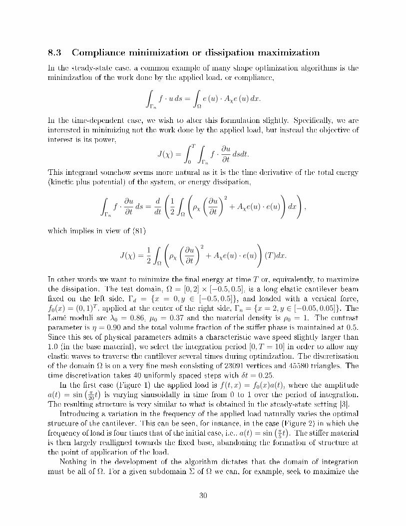
In other words we want to minimize the nal energy at time T or, equivalently, to maximizethe dissipation. The test domain, Ω = [0, 2] × [−0.5, 0.5], is a long elastic cantilever beamxed on the left side, Γd = x = 0, y ∈ [−0.5, 0.5], and loaded with a vertical force,f0(x) = (0, 1)T , applied at the center of the right side, Γn = x = 2, y ∈ [−0.05, 0.05]. TheLamé moduli are λ0 = 0.86, µ0 = 0.37 and the material density is ρ0 = 1. The contrastparameter is η = 0.90 and the total volume fraction of the stier phase is maintained at 0.5.Since this set of physical parameters admits a characteristic wave speed slightly larger than1.0 (in the base material), we select the integration period [0, T = 10] in order to allow anyelastic waves to traverse the cantilever several times during optimization. The discretizationof the domain Ω is on a very ne mesh consisting of 23091 vertices and 45580 triangles. Thetime discretization takes 40 uniformly spaced steps with δt = 0.25.
In the rst case (Figure 1) the applied load is f(t, x) = f0(x)a(t), where the amplitudea(t) = sin
(π20t)is varying sinusoidally in time from 0 to 1 over the period of integration.
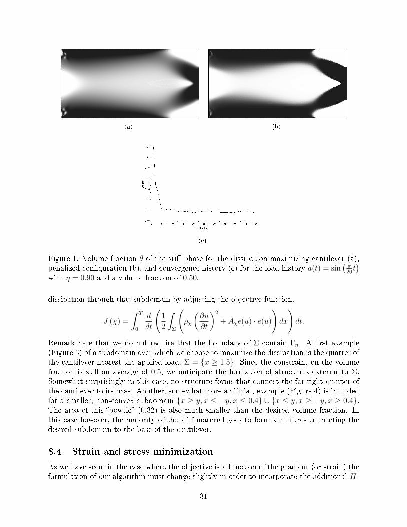
The resulting structure is very similar to what is obtained in the steady-state setting [3].Introducing a variation in the frequency of the applied load naturally varies the optimal
structure of the cantilever. This can be seen, for instance, in the case (Figure 2) in which thefrequency of load is four times that of the initial case, i.e., a(t) = sin
(π5t). The stier material
is then largely realligned towards the xed base, abandoning the formation of structure atthe point of application of the load.
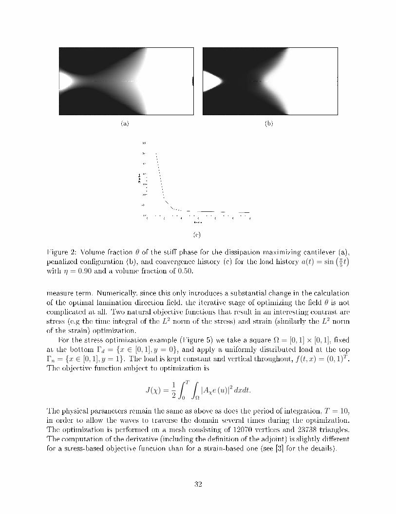
Nothing in the development of the algorithm dictates that the domain of integrationmust be all of Ω. For a given subdomain Σ of Ω we can, for example, seek to maximize the
30
(a) (b)
(c)
Figure 1: Volume fraction θ of the sti phase for the dissipation maximizing cantilever (a),penalized conguration (b), and convergence history (c) for the load history a(t) = sin
(π20t)
with η = 0.90 and a volume fraction of 0.50.
dissipation through that subdomain by adjusting the objective function.
J (χ) =
∫ T
0
d
dt
(1
2
∫Σ
(ρχ
(∂u
∂t
)2
+ Aχe(u) · e(u)
)dx
)dt.
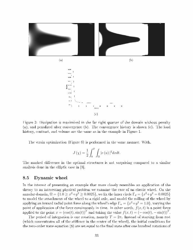
Remark here that we do not require that the boundary of Σ contain Γn. A rst example(Figure 3) of a subdomain over which we choose to maximize the dissipation is the quarter ofthe cantilever nearest the applied load, Σ = x ≥ 1.5. Since the constraint on the volumefraction is still an average of 0.5, we anticipate the formation of structures exterior to Σ.Somewhat surprisingly in this case, no structure forms that connect the far right quarter ofthe cantilever to its base. Another, somewhat more articial, example (Figure 4) is includedfor a smaller, non-convex subdomain x ≥ y, x ≤ −y, x ≤ 0.4 ∪ x ≤ y, x ≥ −y, x ≥ 0.4.The area of this bowtie (0.32) is also much smaller than the desired volume fraction. Inthis case however, the majority of the sti material goes to form structures connecting thedesired subdomain to the base of the cantilever.
8.4 Strain and stress minimization
As we have seen, in the case where the objective is a function of the gradient (or strain) theformulation of our algorithm must change slightly in order to incorporate the additional H-
31
(a) (b)
(c)
Figure 2: Volume fraction θ of the sti phase for the dissipation maximizing cantilever (a),penalized conguration (b), and convergence history (c) for the load history a(t) = sin
(π5t)
with η = 0.90 and a volume fraction of 0.50.
measure term. Numerically, since this only introduces a substantial change in the calculationof the optimal lamination direction eld, the iterative stage of optimizing the eld θ is notcomplicated at all. Two natural objective functions that result in an interesting contrast arestress (e.g the time integral of the L2 norm of the stress) and strain (similarly the L2 normof the strain) optimization.
For the stress optimization example (Figure 5) we take a square Ω = [0, 1]× [0, 1], xedat the bottom Γd = x ∈ [0, 1], y = 0, and apply a uniformly distributed load at the topΓn = x ∈ [0, 1], y = 1. The load is kept constant and vertical throughout, f(t, x) = (0, 1)T .The objective function subject to optimization is
J(χ) =1
2
∫ T
0
∫Ω
|Aχe (u)|2 dxdt.
The physical parameters remain the same as above as does the period of integration, T = 10,in order to allow the waves to traverse the domain several times during the optimization.The optimization is performed on a mesh consisting of 12070 vertices and 23738 triangles.The computation of the derivative (including the denition of the adjoint) is slightly dierentfor a stress-based objective function than for a strain-based one (see [3] for the details).
32
(a) (b)
(c)
Figure 3: Dissipation is maximized in the far right quarter of the domain without penalty(a), and penalized after convergence (b). The convergence history is shown (c). The loadhistory, contrast, and volume are the same as in the example in Figure 1.
The strain optimization (Figure 6) is performed in the same manner. With,
J (χ) =1
2
∫ T
0
∫Ω
|e (u) |2dxdt.
The marked dierence in the optimal structures is not surprising compared to a similaranalysis done in the elliptic case in [3].
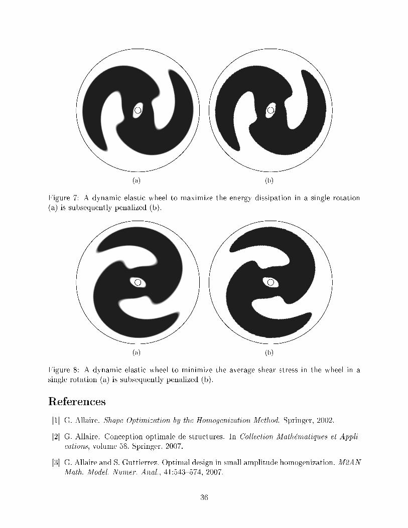
8.5 Dynamic wheel
In the interest of presenting an example that more closely resembles an application of thetheory to an interesting physical problem we examine the case of an elastic wheel. On theannular domain, Ω = 1.0 ≥ x2+y2 ≥ 0.0025, we x the inner circle Γd = x2+y2 = 0.0025to model the attachment of the wheel to a rigid axle, and model the rolling of the wheel byapplying an inward radial point force along the wheel's edge Γn = x2+y2 = 1.0, varying thepoint of application of the force continuously in time. In other words, f(x, t) is a point forceapplied to the point x = (cos(t), sin(t))T and taking the value f(x, t) = (− cos(t),− sin(t))T .
The period of integration is one rotation, namely T = 2π. Instead of starting from rest(which concentrates all of the stiener in the center of the wheel), the initial conditions forthe zero-order wave equation (8) are set equal to the nal state after one hundred rotations of
33

(a) (b)
(c)
Figure 4: Dissipation is maximized in the bowtie subdomain without penalty (a), andpenalized after convergence (b). The convergence history is shown (c). The load history,contrast, and volume are the same as in the example in Figure 1.
the wheel (so it is almost a time periodic solution). Thus optimization begins with non-zeroinitial data, contrary to the previous examples. The volume fraction of the stier phase ismaintained at 0.5.
We examine two objective functions: maximization of the dissipation (Figure 7),
J (χ) =
∫ T
0
∫Ω
(ρχ∂2u
∂t2· ∂u∂t− div (Aχe (u)) · ∂u
∂t
)dxdt,
and minimization of the shear stress (Figure 8),
J (χ) =
∫ T
0
∫Ω
1
2σ12 (u) : σ12 (u) dxdt,
on a ne mesh of 14306 vertices and 28192 triangles.The results of Figures 7 and 8 are very similar, up to a 90 degrees rotation. Because of
our initial conditions which somehow approximate time periodic boundary conditions, it isexpected that a non radial optimal design can not be unique since any rotation of it willyield a new optimal design.
34
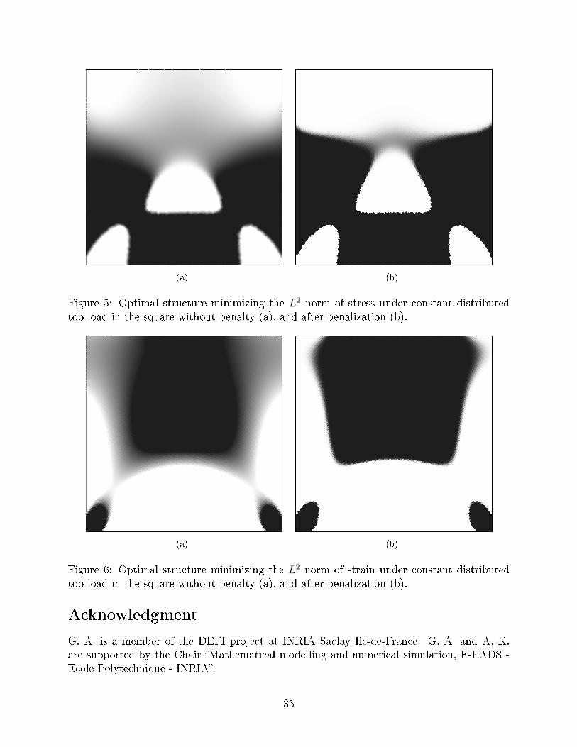
(a) (b)
Figure 5: Optimal structure minimizing the L2 norm of stress under constant distributedtop load in the square without penalty (a), and after penalization (b).
(a) (b)
Figure 6: Optimal structure minimizing the L2 norm of strain under constant distributedtop load in the square without penalty (a), and after penalization (b).
Acknowledgment
G. A. is a member of the DEFI project at INRIA Saclay Ile-de-France. G. A. and A. K.are supported by the Chair Mathematical modelling and numerical simulation, F-EADS -Ecole Polytechnique - INRIA.
35
(a) (b)
Figure 7: A dynamic elastic wheel to maximize the energy dissipation in a single rotation(a) is subsequently penalized (b).
(a) (b)
Figure 8: A dynamic elastic wheel to minimize the average shear stress in the wheel in asingle rotation (a) is subsequently penalized (b).
References
[1] G. Allaire. Shape Optimization by the Homogenization Method. Springer, 2002.
[2] G. Allaire. Conception optimale de structures. In Collection Mathématiques et Appli-cations, volume 58. Springer, 2007.
[3] G. Allaire and S. Guttierrez. Optimal design in small amplitude homogenization. M2ANMath. Model. Numer. Anal., 41:543574, 2007.
36
[4] M. Bendsoe and O. Sigmund. Topology Optimization: Theory, Methods, and Applica-tions. Springer, 2003.
[5] B. Bourdin and R. V. Kohn. Optimization of structural topology in the high-porosityregime. J. Mech. Phys. Solids, 56:10431064, 2008.
[6] S. Brahim-Otsmane, G. Francfort, and F. Murat. Correctors for the homogenization ofthe wave and heat equations. J. Math. Pures Appl., 9:197231, 1992.
[7] L. C. Evans. Partial Dierential Equations. AMS, 1997.
[8] P. Gérard. Microlocal defect measures. Comm. Partial Dierential Equations, 16:17611794, 1991.
[9] F. Hecht, O. Pironneau, and K. Ohtsuka. FreeFEM++: User's Manual.http://www.freefem.org.
[10] R. Kohn. The relaxation of a double-well energy. Contin. Mech. Thermodyn., 3:193236,1991.
[11] A. Larsen, B. Laksafoss, J. S. Jensen, and O. Sigmund. Topological material layoutin plates for vibration supression and wave propagation control. Struct. Multidiscip.Optim., 37:585594, 2009.
[12] J.-L. Lions and E. Magenes. Non-homogeneous Boundary Value Problems and Applica-tions I. Springer, 1972.
[13] K. Lurie. An Introduction to the Mathematical Theory of Dynamic Materials. Springer,2007.
[14] G. Milton. The Theory of Composites. Cambridge University Press, 2001.
[15] A. Munch, P. Pedregal, and F. Periago. Optimal design of the damping set for thestabilization of the wave equation. J. Dierential Equations, 231:331358, 2006.
[16] A. Munch, P. Pedregal, and F. Periago. Relaxation of an optimal design problem forthe heat equation. J. Math. Pures Appl., 89:225247, 2008.
[17] L. Tartar. H-measures, a new approach for studying homogenisation, oscillations, andconcentration eects in partial dierential equations. Proc. Roy. Soc. Edinburgh Sect.A, 115A:193230, 1990.
[18] L. Tartar. An introduction to the homogenization method in optimal design. In A. Cel-lina and A. Ornelas, editors, Optimal Shape Design (Tróia, 1998): Lecture Notes inMathematics 1740, pages 47156. Springer, 2000.
37