optimal design of periodic functionally graded composites

Struct Multidisc Optim (2009) 38:469–489DOI 10.1007/s00158-008-0300-1

RESEARCH PAPER

Optimal design of periodic functionally gradedcomposites with prescribed properties

Glaucio H. Paulino · Emílio Carlos Nelli Silva ·Chau H. Le

Received: 6 July 2007 / Revised: 10 May 2008 / Accepted: 5 July 2008 / Published online: 23 September 2008© Springer-Verlag 2008

Abstract The computational design of a compositewhere the properties of its constituents change grad-ually within a unit cell can be successfully achievedby means of a material design method that combinestopology optimization with homogenization. This is aniterative numerical method, which leads to changes inthe composite material unit cell until desired proper-ties (or performance) are obtained. Such method hasbeen applied to several types of materials in the lastfew years. In this work, the objective is to extend thematerial design method to obtain functionally gradedmaterial architectures, i.e. materials that are graded atthe local level (e.g. microstructural level). Consistentwith this goal, a continuum distribution of the designvariable inside the finite element domain is consideredto represent a fully continuous material variation dur-ing the design process. Thus the topology optimizationnaturally leads to a smoothly graded material system.To illustrate the theoretical and numerical approaches,numerical examples are provided. The homogenizationmethod is verified by considering one-dimensional ma-terial gradation profiles for which analytical solutionsfor the effective elastic properties are available. The

G. H. Paulino · C. H. LeDepartment of Civil and Environmental Engineering,University of Illinois at Urbana-Champaign,Newmark Laboratory, 205 North Mathews Avenue,Urbana, IL 61801, USA

E. C. N. Silva (B)Department of Mechatronics and Mechanical Systems,Escola Politécnica da Universidade de São Paulo,Av. Professor Mello Moraes, 2231,São Paulo, São Paulo 05508-900, Brazile-mail: [email protected]

verification of the homogenization method is extendedto two dimensions considering a trigonometric materialgradation, and a material variation with discontinuousderivatives. These are also used as benchmark exam-ples to verify the optimization method for functionallygraded material cell design. Finally the influence ofmaterial gradation on extreme materials is investigated,which includes materials with near-zero shear modulus,and materials with negative Poisson’s ratio.

Keywords Material design · Functionally gradedmaterials · Optimization · Homogenization ·Extreme materials · Zero shear-modulus materials ·Negative Poisson’s ratio materials

Nomenclature

List of Symbols:

A assembling operatorD elasticity tensorDijkl index notation for elasticity tensorD∗

ijkl index notation for desired tensorproperties

DH homogenized tensor propertiesDH

rspq index notation for homogenized tensorproperties

DHij matrix notation for homogenized tensor

propertiesDm elasticity tensor of the mixturedn design variables associated with nodesEm Young’s modulus of mixtureE+, E− Young’s modulus of materials + and −

470 G.H. Paulino et al.

e element ef projection functionF(mn) nodal force vector for load case mnFe(mn)

iI component of nodal force vector for loadcase mn

Fe(mn) finite element nodal force vector for loadcase mn

G shear modulusGmax, Gmin upper and lower limits of shear modulusGm shear modulus of the mixtureG+, G− shear modulus of materials + and −Hper set of Y-periodic functionsi, j, k, l indicesI identity tensorI indexK stiffness matrixKe finite element stiffness matrixKe

(iI jJ) term of finite element stiffness matrixK bulk modulusKmax, Kmin upper and lower limits of bulk modulusKm bulk modulus of the mixtureK+, K− bulk modulus of materials + and −mI elements associated with I-th nodemn load case numberNI finite element shape functionN number of finite elementsnd number of nodes per finite elementNDV number of design variablesNEXCL number of elements explicitly excluded

from the optimizationrmin radius of circlerij distance between nodes j and iR3 3D space of real numbersSi set of nodes in the domain of influence of

node iuε displacement inside the unit cellu0 zero order term of displacementu1 first-order variation of displacementv displacement vectorVi relative volume of each finite elementvi component of vector vx coordinates associated with the composite

macro-dimensionsx j position vector of node jx, y cartesian coordinatesy coordinates associated with the composite

micro-dimensionsY unit cell domainY unit cell volumeYi maximum value of coordinate i of unit cell

domainW objective function

wijkl weight coefficientw weight function∂ differential operator∂x differential operator for macro

coordinates(∂x)ij (.) index notation for differential operator

for macro coordinates∂ y differential operator for micro

coordinates(∂y

)ij (.) index notation for differential operator

for micro coordinatesχ characteristic displacement function of

the unit cellχ

(mn)

i component of characteristic displacementfunction for load case mn

χ̂ (mn) nodal values of the characteristic functionχ for load case mn

δ variational operatorδim kronecker deltaε strainεε strain inside unit cellεkl index notation for strainε parameter� function of interestκ interpolation factorvm Poisson’s ratio of mixtureν+, ν− Poisson’s ratio of materials + and − averaged volume fractionρ pseudo-density distribution function

(design variable)ρI nodal pseudo-density function

(design variable)ρlow lower bound for design variables ρI

σij index notation for stress domain volume e finite element volume∪ union operator

1 Introduction

Functionally Graded Materials (FGMs) possess con-tinuously graded properties and are characterized byspatially varying microstructures created by nonuni-form distributions of the reinforcement phase as well asby interchanging the role of reinforcement and matrix(base) materials in a continuous manner. The smoothvariation of properties may offer advantages such aslocal reduction of stress concentration and increasedbonding strength (see, for example, Miyamoto et al.1999; Suresh and Mortensen 1988; Paulino et al. 2003).

Optimal design of periodic functionally graded composites with prescribed properties 471

Standard composites result from the combination oftwo or more materials, usually resulting in materialsthat offer advantages over conventional materials. Theunit cell is the smallest structure that is periodic in thecomposite matrix. By changing the volume fraction ofthe constituents, the shape of the inclusions, or eventhe topology of the unit cell, we can obtain different ef-fective properties for the composite material (Torquato2002). Therefore, when designing composites, we cantailor the properties to a specific application (which, ingeneral, cannot be done with a single material). At themacroscale observation, traditional composites (e.g.laminated) exhibit a sharp interface among the con-stituent phases which may cause problems such as stressconcentration, and scattering (if a wave is propagatinginside the material), among others. However, a materialmade using the FGM concept would maintain some ofthe advantages of traditional composites and alleviateproblems related to the presence of sharp interfaces atthe macroscale. The design of the composite materialitself is a difficult task, and the design of a compositewhere the properties of its constituent materials changegradually in the unit cell domain is even more complex.Meanwhile, this design can be successfully achieved byusing a material design method, as described below.

The overall objective of material design is to gen-erate composite materials with prescribed or improvedproperties not found in common materials. This can beachieved by modifying the microstructure of the com-posite material (Torquato 2002). In traditional com-posite designs, such as fiber- or sphere-reinforced andlaminated materials, the change in the properties is ob-tained by modifying the location, orientation, materialconstituents, or volume fraction of the fiber, sphere,or laminar inclusion, respectively (Cherkaev and Kohn1997). This allows some control of the composite prop-erties. A more systematic approach to design compositematerials has been developed in recent years, whichcombines topology optimization with homogenizationto change the composite material unit cell topologyuntil desired properties or performance are obtained.The approach consists of finding the distribution ofdifferent material phases in a periodic unit cell thatoptimizes the properties or performance characteristicsof the resulting composite system (Cherkaev and Kohn1997; Cherkaev 2000).

In the process of designing materials with prescribedand improved properties, a natural question related tothe achievable properties in the material design processarises. Based on the fact that the constitutive elasticitymatrix must be positive definite for elastic materials,Milton and Cherkaev (1995) have shown the existence

of materials for thermodynamically admissible sets bylayering and combining an infinitely rigid materialwith voids (infinite compliance). However, the extremecondition of this admissible set, such as isotropic mater-ial with Poisson’s ratio equal to −1 (ν = −1), cannot bereached in practice because an infinitely rigid materialdoes not exist.

Other bounds were derived in the past. Consideringmaterials with finite properties, we can cite, for ex-ample, the work of Hashin and Shtrikman (1963) forbounds of an isotropic mixture of classical materialsusing energy analyses, the work of Lipton and Northrup(1994) (among others) that defined the bounds for or-thotropic mixtures of isotropic materials, and the workof Cherkaev and Gibiansky (1993) that improved theclassical Hashin and Shtrikman (1963) estimates of theeffective properties for an isotropic mixture assembledfrom two isotropic elastic materials. Bounds for elas-ticity and conductivity properties of mixtures of twomaterials (not necessarily isotropic) were developed byGibiansky and Torquato (1995) and Cherkaev andGibiansky (1996). Attainable properties for piezoelec-tric materials were discussed by Smith (1992) consid-ering the positive definiteness of a tensor involvingelastic, piezoelectric, and dielectric properties, how-ever, no bounds were obtained. Gibiansky andTorquato (1999) also discussed optimal bounds forpiezoelectric matrix laminate composites. However, theextremal properties that can be achievable by compos-ite designs is limited, and has been explored mainly forelasticity and conductivity (Sigmund 2000; Cherkaevand Gibiansky 1993; Gibiansky and Sigmund 2000;Larsen et al. 1997).

In the past few years, the material design conceptbased on topology optimization and homogenizationhas been applied to design elastic (Sigmund 1994, 1995;Neves et al. 2002; Diaz and Benard 2003; Guedes et al.2003; Neves et al. 2000), thermoelastic (Sigmund andTorquato 1996, 1997; Chen et al. 2001; Torquato et al.2003), piezoelectric (Silva et al. 1998, 1999a, b; Sigmundet al. 1998; Sigmund and Torquato 1999), phononic(Sigmund and Jensen 2003), and photonic (Cox andDobson 1999, 2000) composite materials, among oth-ers. In addition, manufacturing techniques have alsobeen studied to build such materials (Qi and Halloran2004; Van Hoy et al. 1998; Crumm and Halloran 1998;Qi et al. 2004; Mazumder et al. 1999, 2000; Crumm et al.2007). However, processing techniques have not beenexplored when material gradation is considered insidethe unit cell, and have concentrated in the traditional(1–0) design (Qi et al. 2004; Mazumder et al. 2000). Thispaper explores the computational design of periodic


functionally graded microstructures. The manufactur-ing of such materials is beyond the scope of the presentwork and is a subject of future research.

This paper is organized as follows. In Section 2, abrief introduction about topology optimization for FGMstructures is given. In Section 3, the theoretical formu-lation of homogenization for FGM composite materialsis addressed. In Section 4, the formulation of the com-posite material design problem based on continuoustopology optimization is presented, and in Section 5the material model applied is described. The numericalimplementation, including an applied gradient controlfor material gradation, is discussed in Section 6. Thesensitivity analysis is briefly described in Section 7. InSection 8, some representative results are presentedto illustrate homogenization and material design con-cepts. The influence of FGM gradation in the design ofextreme materials such as minimum shear stiffness andnegative Poisson’s ratio materials is discussed. Finally,in Section 9, concluding remarks are provided.

2 Topology optimization

A major concept in topology optimization is the ex-tended design domain, which is a large fixed domainthat must contain the whole structure to be determinedby the optimization procedure. The objective is to de-termine the holes and connectivities of the structure byadding and removing material in this domain. Becausethe extended domain is fixed, the finite element modelis not changed during the optimization process, whichsimplifies the calculation of derivatives of functions de-fined over the extended domain (Bendsøe and Kikuchi1988; Allaire 2002). In the case of material design, theextended design domain is the unit cell domain.

The discrete problem, where the amount of materialat each element can assume only values equal to eitherone or zero (i.e. void or solid material, respectively),is an ill-posed problem. A typical way to seek a solu-tion for topology optimization problems is to relax theproblem by allowing the material to assume intermedi-ate property values during the optimization procedure,which can be achieved by defining a special materialmodel (Cherkaev 2000; Allaire 2002; Kohn and Strang1986a, b, c; Murat and Tartar 1985). Essentially, the ma-terial model approximates the material distribution bydefining a function of a continuous parameter (designvariable) that determines the mixture of basic materialsthroughout the domain. In this sense, the relaxationyields a continuous material design problem that nolonger involves a discernible connectivity. A topol-ogy solution can be obtained by applying penalization

coefficients to the material model to recover the 0–1design (and thus, a discernible connectivity), and somegradient control on material distribution, such as a filteror projection (Bendsøe and Sigmund 2003).

It turns out that this relaxed problem is stronglyrelated to the FGM design problem, which essentiallyseeks a continuous transition of material properties(Paulino and Silva 2005; Silva and Paulino 2004). Thus,while the 0–1 design problem (needs complexity con-trol, such as filter) does not admit intermediate valuesof design variables, the FGM design problem admitsolutions with intermediate values of the material field.

Early work on material design followed a tradi-tional topology optimization formulation, where thedesign variables are defined in a piecewise fashion inthe discretized domain, which means that continuityof the material distribution is not realized betweenfinite elements. However, considering that the topologyoptimization results in a smoothly graded material, amore natural way of representing the material distrib-ution emerges by considering a continuous representa-tion of material properties (Matsui and Terada 2004;Rahmatalla and Swan 2004), which is achieved by inter-polating the properties inside the finite element usingshape functions (Matsui and Terada 2004; Rahmatallaand Swan 2003; Guest et al. 2004). The concept ofemploying continuum interpolation of material distri-bution inside the finite element has been implementedto model FGMs, originating the so-called “graded finiteelement” (Kim and Paulino 2002) . Thus, nodal designvariables are defined rather than the usual elementbased design variables.

The objective of the present work is to design FGMcomposites using the concept of the relaxed problem incontinuum topology optimization. Thus, the design ofelastic FGM composites to achieve desired propertiesis addressed. The problem is posed by minimizing thesquare difference between homogenized and desiredproperties. A continuum distribution of the designvariable inside the finite element domain is consid-ered allowing representation of a continuous mate-rial variation during the design process. Since we areinterested in solutions with a continuous distributionof material, we allow for intermediate materials (nopenalization). A material model based on the Hashinand Shtrikman bounds is employed to guarantee thatthe final composite can be achieved by a mixture ofbasic materials used in the design. A gradient controlconstraint in the unit cell domain is implemented basedon projection techniques (Guest et al. 2004; Carbonariet al. 2007). This gradient control capability permits toaddress the influence of FGM gradation in the designof extreme materials. It also avoids the problem of


mesh dependency in the topology optimization imple-mentation (Bendsøe and Sigmund 2003). The actualoptimization problem is solved by the MMA (“Methodof Moving Assymptotes”) algorithm (Svanberg 1987;Bruyneel et al. 2002).

3 Homogenization method

Homogenization allows the calculation of the effectiveproperties of a complex periodic composite materialfrom its unit cell topology. It is a general method forcalculating effective properties and has no limitationsregarding volume fraction or shape of the compositeconstituents. The main assumptions are that the unitcell is periodic and that the scale of the compositepart is much larger than the microstructure dimensions(Cherkaev and Kohn 1997; Allaire 2002; Guedes andKikuchi 1990).

This section addresses details of the theoretical andcomputational aspects of the homogenization methodapplied to FGM composites. Considering the standardhomogenization procedure for elastic materials, theunit cell is defined as Y = [0, Y1] × [0, Y2] × [0, Y3] andthe elastic property function Dijkl is considered to be aY-periodic function:

Dε(x) = D(x, y); D(x, y) = D(x, y+Y)

and y = x/ε , ε > 0, (1)

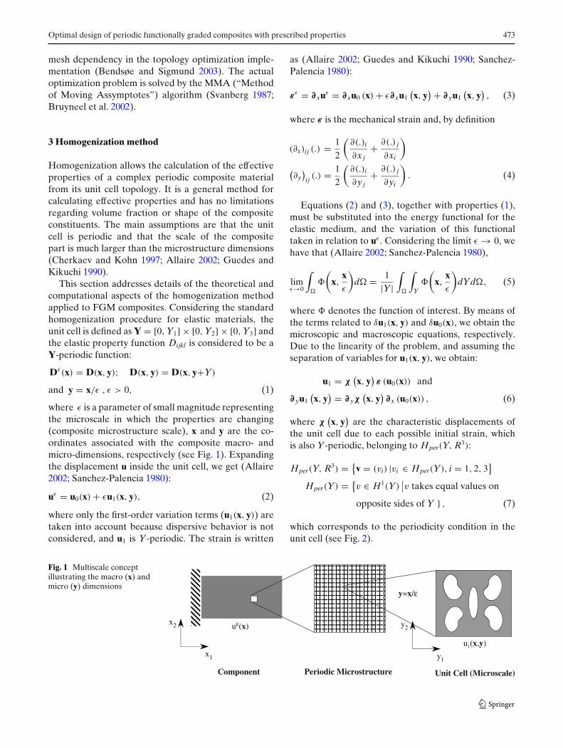
where ε is a parameter of small magnitude representingthe microscale in which the properties are changing(composite microstructure scale), x and y are the co-ordinates associated with the composite macro- andmicro-dimensions, respectively (see Fig. 1). Expandingthe displacement u inside the unit cell, we get (Allaire2002; Sanchez-Palencia 1980):

uε = u0(x) + εu1(x, y), (2)

where only the first-order variation terms (u1(x, y)) aretaken into account because dispersive behavior is notconsidered, and u1 is Y-periodic. The strain is written

as (Allaire 2002; Guedes and Kikuchi 1990; Sanchez-Palencia 1980):

εε = ∂xuε = ∂xu0 (x) + ε∂xu1(x, y

) + ∂ yu1(x, y

), (3)

where ε is the mechanical strain and, by definition

(∂x)ij (.) = 1

2

(∂(.)i

∂x j+ ∂(.) j

∂xi

)

(∂y

)ij (.) = 1

2

(∂(.)i

∂y j+ ∂(.) j

∂yi

). (4)

Equations (2) and (3), together with properties (1),must be substituted into the energy functional for theelastic medium, and the variation of this functionaltaken in relation to uε . Considering the limit ε → 0, wehave that (Allaire 2002; Sanchez-Palencia 1980),

limε→0

∫

�

(x,

xε

)d = 1

|Y|∫

∫

Y�

(x,

xε

)dYd , (5)

where � denotes the function of interest. By means ofthe terms related to δu1(x, y) and δu0(x), we obtain themicroscopic and macroscopic equations, respectively.Due to the linearity of the problem, and assuming theseparation of variables for u1(x, y), we obtain:

u1 = χ(x, y

)ε (u0(x)) and

∂ yu1(x, y

) = ∂ yχ(x, y

)∂x (u0(x)) , (6)

where χ(x, y

)are the characteristic displacements of

the unit cell due to each possible initial strain, whichis also Y-periodic, belonging to Hper(Y, R3):

Hper(Y, R3) = {v = (vi) |vi ∈ Hper(Y), i = 1, 2, 3

}

Hper(Y) = {v ∈ H1(Y)

∣∣v takes equal values on

opposite sides of Y } , (7)

which corresponds to the periodicity condition in theunit cell (see Fig. 2).

Fig. 1 Multiscale conceptillustrating the macro (x) andmicro (y) dimensions

y1

y2

x1

x2 uε(x)

u1(x,y)

y=x/ε

Component Periodic Microstructure Unit Cell (Microscale)


Periodicity ConditionsUnit Cell

Fig. 2 Periodicity conditions in the unit cell

Therefore, substituting (6) into the microscopicequations, we obtain (Allaire 2002; Guedes andKikuchi 1990; Sanchez-Palencia 1980):

1

|Y|∫

Y

[(I + ∂ yχ

(x, y

)) : D(x, y

) : ∂ yδu1(x, y)]

dY = 0,

∀δu1 ∈ Hper(Y, R3), (8)

which can be rewritten using the index notation:

1

|Y|∫

YDijkl

(x, y

)(

δimδ jn + ∂χ(mn)

i

∂y j

)

εkl (v) dY = 0,

∀v ∈ Hper(Y, R3). (9)

Substituting (6) into the macroscopic equations,we obtain the definition of the effective properties(Allaire 2002; Guedes and Kikuchi 1990; Sanchez-Palencia 1980):

DH = 1

|Y|∫

Y

[D

(x, y

) : (I + ∂ yχ

(x, y

))]dY. (10)

By using (8), one can easily show that (10) can also bewritten in the form:

DH = 1

|Y|∫

Y

[(I + ∂ yχ

(x, y

)) : D(x, y

)

: (I + ∂ yχ

(x, y

))]dY, (11)

or using the index notation:

DHrspq (x) = 1

|Y|∫

YDijkl

(x, y

)(

δipδ jq + ∂χ(pq)

i

∂y j

)

×(

δkrδls + ∂χ(rs)k

∂yl

)

dY, (12)

where DHijkl = DH

klij = DHjikl.

Table 1 Boundary conditions for faces (2D plane-stress)

Load cases b.c. at y1 = 0, y1 = Y1 b.c. at y2 = 0, y2 = Y2

m = n (1 or 2) χ(mn)1 = 0; σ21 = 0 χ

(mn)2 = 0; σ21 = 0

mn = 12 (or 21) χ(12)2 = 0; σ11 = 0 χ

(12)1 = 0; σ22 = 0

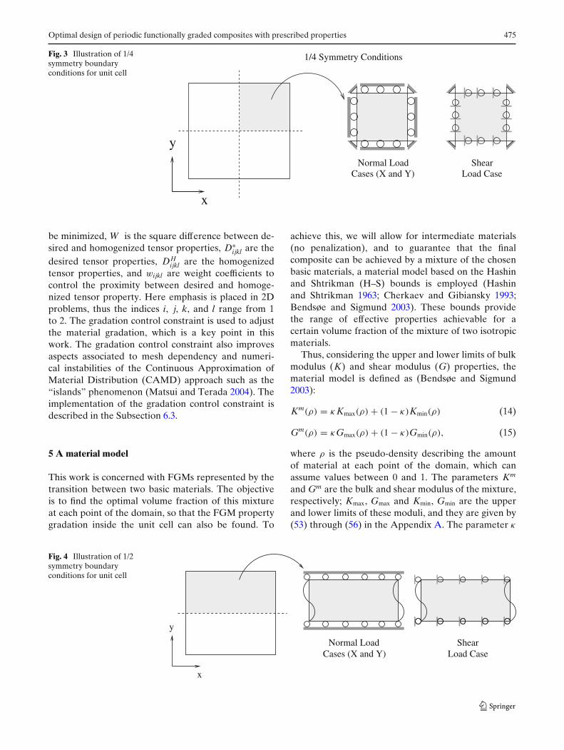
The calculation of effective properties can becomecomputationally efficient by taking advantage of sym-metry boundary conditions. An isotropic unit cell hassymmetry relative to all axes; and an orthotropic unitcell has symmetry relative to either both axes or onlyone axis. In this case, we can take advantage of theseproperties to reduce the computational cost and to con-duct the optimization and homogenization in only onepart of the domain. However, the appropriate bound-ary conditions must be considered for the displacementcharacteristic function χ . For a 2D plane-strain case,Table 1 describes the boundary conditions that must bespecified when only one fourth or half of the unit cell isconsidered (Silva et al. 1998), as described in Figs. 3 and4, respectively. For the half symmetry case, the actualconditions to be employed must be taken according tothe type of symmetry (along x-axis as in Fig. 4 or alongthe y-axis).

4 Material design method

The material design optimization problem consists offinding a distribution of material inside the unit cell thatwill achieve specified homogenized properties. Thisproblem is also known as the inverse homogenizationproblem (Cherkaev 2000; Sigmund 1994; Bendsøe andSigmund 2003). The optimization problem consists ofminimizing a cost function related to the density dis-tribution inside the unit cell subjected to equality con-straints on the elastic properties. Thus, the optimizationproblem can be stated in continuous form as follows(Sigmund 1994, 1995):

Minimize :ρ(x)

W (ρ) =2∑

i, j,k,l=1

wijkl

(D∗

ijkl − DHijkl

)2

Subjected to : 1

|Y|∫

Y

[(I + ∂ yχ

(x, y

)) : D(x, y

) :

∂ yδu1(x, y)]

dY = 0

∀δu1 ∈ Hper(Y, R3)

0 ≤ ρ(x) ≤ 1

gradation control, (13)

where ρ(x) is the pseudo-density distribution functionalong the unit cell domain, W(ρ) is a cost function to


Fig. 3 Illustration of 1/4symmetry boundaryconditions for unit cell

Load CaseShear

Cases (X and Y)Normal Load

y

x

1/4 Symmetry Conditions

be minimized, W is the square difference between de-sired and homogenized tensor properties, D∗

ijkl are thedesired tensor properties, DH

ijkl are the homogenizedtensor properties, and wijkl are weight coefficients tocontrol the proximity between desired and homoge-nized tensor property. Here emphasis is placed in 2Dproblems, thus the indices i, j, k, and l range from 1to 2. The gradation control constraint is used to adjustthe material gradation, which is a key point in thiswork. The gradation control constraint also improvesaspects associated to mesh dependency and numeri-cal instabilities of the Continuous Approximation ofMaterial Distribution (CAMD) approach such as the“islands” phenomenon (Matsui and Terada 2004). Theimplementation of the gradation control constraint isdescribed in the Subsection 6.3.

5 A material model

This work is concerned with FGMs represented by thetransition between two basic materials. The objectiveis to find the optimal volume fraction of this mixtureat each point of the domain, so that the FGM propertygradation inside the unit cell can also be found. To

achieve this, we will allow for intermediate materials(no penalization), and to guarantee that the finalcomposite can be achieved by a mixture of the chosenbasic materials, a material model based on the Hashinand Shtrikman (H–S) bounds is employed (Hashinand Shtrikman 1963; Cherkaev and Gibiansky 1993;Bendsøe and Sigmund 2003). These bounds providethe range of effective properties achievable for acertain volume fraction of the mixture of two isotropicmaterials.

Thus, considering the upper and lower limits of bulkmodulus (K) and shear modulus (G) properties, thematerial model is defined as (Bendsøe and Sigmund2003):

Km(ρ) = κKmax(ρ) + (1 − κ)Kmin(ρ) (14)

Gm(ρ) = κGmax(ρ) + (1 − κ)Gmin(ρ), (15)

where ρ is the pseudo-density describing the amountof material at each point of the domain, which canassume values between 0 and 1. The parameters Km

and Gm are the bulk and shear modulus of the mixture,respectively; Kmax, Gmax and Kmin, Gmin are the upperand lower limits of these moduli, and they are given by(53) through (56) in the Appendix A. The parameter κ

Fig. 4 Illustration of 1/2symmetry boundaryconditions for unit cell

ShearCases (X and Y)

Normal Load

y

x

Load Case


is an interpolation factor to define a curve interpolatingthe upper and lower limits of bulk and shear modulus.In this work, κ = 0.5. The basic materials of the mixturewill be designated by the symbols (+) and (−). Theyhave bulk and shear modulus equal to K+, K− and G+,G−, respectively, such that K+ > K− and G+ > G−.The values of Kmax, Kmin, Gmax, and Gmin are functionsof those properties (Appendix A). For ρ equal to 0 thematerial is equal to material (−) and for ρ equal to 1 itis equal to material (+).

The Young’s modulus (Em) and Poisson’s ratio (νm)of the mixture can be written as a function of Km andGm through the expressions:

Em(ρ) = 9Km(ρ)

1 + 3 Km(ρ)

Gm(ρ)

; νm(ρ) = 1 − 2/3 Gm(ρ)

Km(ρ)

2 + 2/3 Gm(ρ)

Km(ρ)

. (16)

Regarding the capability of traditional microme-chanical models to evaluate effective properties, Reiteret al. (1997) have investigated the Mori-Tanaka andSelf-consistent models to estimate these properties.Their main conclusion is that these models can be ap-plied to the regions where the inclusion and the matrixphases can be easily distinguished. For the transitionregion, these models may be valid depending on theratio of phase properties.

The use of traditional micromechanical models forFGMs has been questioned in the literature because thecontinuous transition of microstructure causes a non-uniform macroscopic distribution of properties. Thustraditional approaches have limitations, and the readeris referred to the technical literature in the subject(Pindera et al. 1995; Yin et al. 2004). The computationalframework presented here is general, and thus othermaterial models can easily replace the present onebased on H-S bounds (which assumes that the FGMgradation law is smooth enough for its application).

6 Numerical implementation

The concept of the continuum distribution of designvariable based on the CAMD method (Matsui andTerada 2004; Rahmatalla and Swan 2004) discussedabove is considered. Thus, (14) and (15) are consideredfor each node, and the pseudo-density (ρ) inside eachfinite element is given by

ρ (x) =nd∑

I=1

ρI NI, (17)

where ρI is the nodal design variable, NI is the fi-nite element shape function that must be selected toprovide non-negative values of the design variables,

and nd is the number of nodes at each element (forexample, four in the 2D case). This formulation allowsa continuous distribution of material along the designdomain instead of the traditional piecewise constantmaterial distribution applied by previous formulationsof topology optimization (Bendsøe and Sigmund 2003).

6.1 Homogenization

The numerical implementation of homogenization ispresented considering the CAMD concept. Equation(8) is solved using FEM. The unit cell is discretized byN finite elements, thus:

Y = ∪Ne=1

e, (18)

where e is the domain of each element. A four-node bilinear element with two displacements degreesof freedom per node that uses bilinear interpolationfunctions was applied. Thus, the characteristic functionspreviously defined are expressed at each element usingthe shape functions (NI):

χ(mn)

i∼=

nd∑

I=1

NIχ(mn)

iI , (19)

Similar relations hold for the virtual displacement v.Substituting (19) in (8), and assembling the individualmatrices for each element, we obtain the followingglobal matrix system for each load case mn:

Kχ̂ (mn) = F(mn), (20)

where χ̂ (mn) are the corresponding nodal values ofthe characteristic function χ , respectively. The globalstiffness is the assembly of each element’s individualmatrix, and the global force (F) is the assembly of theindividual force vectors for all elements.

K = ANe=1Ke; F(mn) = AN

e=1Fe(mn). (21)

The element matrices and vectors are given by theexpressions:

Ke(iI jJ) =

∫

eDipjq

∂ NI

∂yp

∂ NJ

∂yqd e;

Fe(mn)

iI =∫

eDijmn

∂ NI

∂y jd e. (22)

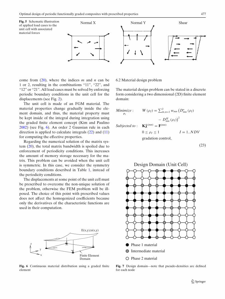
Thus, for the 2D problem, there are three load casesto be solved independently as illustrated in Fig. 5. They


Fig. 5 Schematic illustrationof applied load cases to theunit cell with associatedmaterial forces

Normal X ShearNormal Y

come from (20), where the indices m and n can be1 or 2, resulting in the combinations “11”, “22”, and“12” or “21”. All load cases must be solved by enforcingperiodic boundary conditions in the unit cell for thedisplacements (see Fig. 2).

The unit cell is made of an FGM material. Thematerial properties change gradually inside the ele-ment domain, and thus, the material property mustbe kept inside of the integral during integration usingthe graded finite element concept (Kim and Paulino2002) (see Fig. 6). An order 2 Gaussian rule in eachdirection is applied to calculate integrals (22) and (11)for computing the effective properties.

Regarding the numerical solution of the matrix sys-tem (20), the total matrix bandwidth is spoiled due toenforcement of periodicity conditions. This increasesthe amount of memory storage necessary for the ma-trix. This problem can be avoided when the unit cellis symmetric. In this case, we consider the symmetryboundary conditions described in Table 1, instead ofthe periodicity conditions.

The displacements at some point of the unit cell mustbe prescribed to overcome the non-unique solution ofthe problem, otherwise the FEM problem will be ill-posed. The choice of this point with prescribed valuesdoes not affect the homogenized coefficients becauseonly the derivatives of the characteristic functions areused in their computation.

DomainFinite Element

υ(x,y)E(x,y),

y

z

x

Fig. 6 Continuous material distribution using a graded finiteelement

6.2 Material design problem

The material design problem can be stated in a discreteform considering a two dimensional (2D) finite elementdomain:

Minimize :ρ I

W (ρI) = ∑2m,n=1 wmn

(D∗

mn (ρI)

− DHmn (ρI)

)2

Subjected to : Kχ̂ (mn) = F(mn)

0 ≤ ρI ≤ 1 I = 1..NDV

gradation control,

(23)

Phase 1 material

Design Domain (Unit Cell)

Phase 2 material

Intermediate material

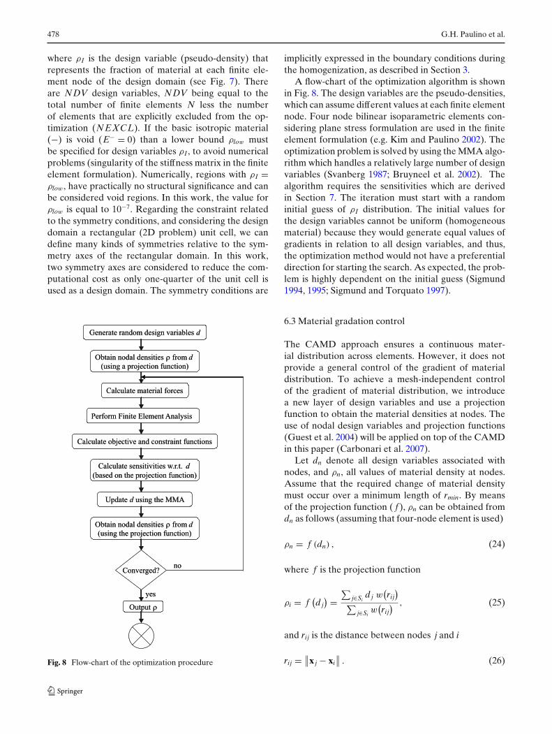
Fig. 7 Design domain—note that pseudo-densities are definedfor each node


where ρI is the design variable (pseudo-density) thatrepresents the fraction of material at each finite ele-ment node of the design domain (see Fig. 7). Thereare NDV design variables, NDV being equal to thetotal number of finite elements N less the numberof elements that are explicitly excluded from the op-timization (NEXCL). If the basic isotropic material(−) is void (E− = 0) than a lower bound ρlow mustbe specified for design variables ρI , to avoid numericalproblems (singularity of the stiffness matrix in the finiteelement formulation). Numerically, regions with ρI =ρlow, have practically no structural significance and canbe considered void regions. In this work, the value forρlow is equal to 10−7. Regarding the constraint relatedto the symmetry conditions, and considering the designdomain a rectangular (2D problem) unit cell, we candefine many kinds of symmetries relative to the sym-metry axes of the rectangular domain. In this work,two symmetry axes are considered to reduce the com-putational cost as only one-quarter of the unit cell isused as a design domain. The symmetry conditions are

Fig. 8 Flow-chart of the optimization procedure

implicitly expressed in the boundary conditions duringthe homogenization, as described in Section 3.

A flow-chart of the optimization algorithm is shownin Fig. 8. The design variables are the pseudo-densities,which can assume different values at each finite elementnode. Four node bilinear isoparametric elements con-sidering plane stress formulation are used in the finiteelement formulation (e.g. Kim and Paulino 2002). Theoptimization problem is solved by using the MMA algo-rithm which handles a relatively large number of designvariables (Svanberg 1987; Bruyneel et al. 2002). Thealgorithm requires the sensitivities which are derivedin Section 7. The iteration must start with a randominitial guess of ρI distribution. The initial values forthe design variables cannot be uniform (homogeneousmaterial) because they would generate equal values ofgradients in relation to all design variables, and thus,the optimization method would not have a preferentialdirection for starting the search. As expected, the prob-lem is highly dependent on the initial guess (Sigmund1994, 1995; Sigmund and Torquato 1997).

6.3 Material gradation control

The CAMD approach ensures a continuous mater-ial distribution across elements. However, it does notprovide a general control of the gradient of materialdistribution. To achieve a mesh-independent controlof the gradient of material distribution, we introducea new layer of design variables and use a projectionfunction to obtain the material densities at nodes. Theuse of nodal design variables and projection functions(Guest et al. 2004) will be applied on top of the CAMDin this paper (Carbonari et al. 2007).

Let dn denote all design variables associated withnodes, and ρn, all values of material density at nodes.Assume that the required change of material densitymust occur over a minimum length of rmin. By meansof the projection function ( f ), ρn can be obtained fromdn as follows (assuming that four-node element is used)

ρn = f (dn) , (24)

where f is the projection function

ρi = f(d j

) =∑

j∈Sid j w

(rij

)

∑j∈Si

w(rij

) , (25)

and rij is the distance between nodes j and i

rij = ∥∥x j − xi∥∥ . (26)


and Si is the set of nodes in the domain under influenceof node i, which consists of a circle of radius rmin andcenter at node i. The weight function w is defined asfollows.

w(rij

) ={ rmin−rij

rminif x j ∈ Si

0 otherwise, (27)

Figure 9 illustrates the idea of the projectiontechnique.

The topology optimization problem definition is re-vised as follows.

Minimize :dI

W (dI) = ∑2m,n=1 wmn

(D∗

mn (dI)

−DHmn (dI)

)2

Subjected to : Kχ̂ (mn) = F(mn)

0 ≤ f (dI) ≤ 1 I = 1..NDV

gradation control.

(28)

Sensitivities with respect to design variables are ob-tained based on those with respect to nodal densitiesusing chain-rule

∂ (.)

∂di=

∑

j∈

∂ (.)

∂ρ j

∂ρ j

∂di, (29)

where is the entire domain, but ∂ρ j/∂di is non-zeroonly at nodes j whose influence domain (S j) containsnode i. Moreover

∂ρ j

∂di= w(rij)∑

k∈S jw(rkj)

. (30)

where ∂ (.) /∂ρ j is obtained by using traditional meth-ods such as the adjoint method, as described in the nextsection.

rmin

i

w(r)

1

rmin rmin

r

Fig. 9 Projection technique concept

7 Sensitivity analysis

To solve the optimization problem defined above, itis necessary to calculate the sensitivity of objectivefunction and constraints in relation to the design vari-ables. The sensitivities of the homogenized propertiesare well-known in the literature (Sigmund 1994, 1995),however, here the formulation is described consideringthe CAMD concept.

Differentiating (11) in relation to the design variableand considering (8), after some algebraic manipulation,we get (Sigmund 1994; Sigmund and Torquato 1997):

∂DH

∂ρI= 1

|Y|∫

Y

[(I + ∂ yχ

(x, y

)) : ∂Dm(x, y

)

∂ρI

: (I + ∂ yχ

(x, y

)) ]dY. (31)

However, considering the material models, given by(14) and (15),

∂Dm(x, y

)

∂ρI= ∂Dm

(x, y

)

∂ρ

∂ρ

∂ρI, (32)

and the continuous distribution of the design variablegiven by (17) inside each finite element is

ρ (x) =nd∑

I=1

ρI NI =⇒ ∂ρ

∂ρI= NI(x). (33)

By discretizing the domain into finite elements, theabove integral will include all mI elements associatedwith I-th node, thus:

∂DH

∂ρI= 1

|Y|mI∑

e=1

[∫

e

[(I+∂ yχ

(x, y

)) : NI(x)∂Dm

(x, y

)

∂ρ

: (I + ∂yχ

(x, y

))]

d e]

. (34)

The calculation of gradients is straightforward and fast(low computational cost) which contributes to the ef-ficiency of the optimization. The calculation of sensi-tivity ∂Dm

(x, y

)/∂ρ is described in Appendix B. In the

case of plane stress, the tensor properties Dm for a two-dimensional problem is given by

Dm = Em

1 − (vm)2

⎡

⎣1 vm 0vm 1 00 0 1−vm

2

⎤

⎦ . (35)


8 Results

To illustrate the theoretical and numerical approaches,numerical examples are provided. The homogenizationmethod is verified by considering one-dimensional ma-terial gradation profiles for which analytical solutionsfor the effective elastic properties are available. Theverification of the homogenization method is also ex-tended to two dimensions considering a trigonometricmaterial gradation, and a material variation with dis-continuous derivatives. These are also used as bench-mark examples to verify the optimization method forFGM cell design. Finally the influence of materialgradation on extreme materials is investigated, whichincludes materials with near-zero shear modulus, andmaterials with negative Poisson’s ratio. The examplesprovided are listed below:

• Verification of homogenization for one-dimensionalgradation

• Homogenization of two-dimensional FGM unitcells

1. Trigonometric material gradation2. Material with discontinuous derivatives

• Optimized FGM cell design

1. Trigonometric material gradation2. Material with discontinuous derivatives3. Near-zero shear modulus materials4. Negative Poisson’s ratio materials

The material design requires the volume fractionof material in the optimization process. The averagedvolume fraction is defined by the expression:

=∫

ρd =⇒ ∼=NDV∑

i=1

ρiVi, (36)

where Vi is the relative volume of each finite elementin the unit cell.

8.1 Verification for one-dimensional gradation

To verify the numerical implementation of the ho-mogenization method for FGM composites, a two-dimensional (2-D) problem with one-dimensionalgradation will be considered (Y = [0, 1]), so that analyt-ical results of the effective properties can be obtained.To ensure that the FGM can be obtained by a mixtureof two materials, the FGM gradation is defined for the

pseudo-density (ρ) and the properties at each point ofthe domain are obtained using the H-S bounds (seeAppendix A). The (idealized) gradation is given by

ρ (x) = (cos 2πx + 1) /2 and 0 ≤ x ≤ 1, (37)

with E+ = 8, ν+ = 0.3, and E− = 1, ν− = 0.3.From reference (Bendsøe and Sigmund 2003), the

effective elastic properties for this type of compositecan be obtained by solving the analytical expressions:

DH11 = 1

∫ 10

1D11

dx; DH

12 =∫ 1

0D12D11

dx∫ 1

01

D11dx

DH22 =

∫ 1

0D22dx −

∫ 1

0

D212

D11dx +

(∫ 10

D12D11

dx)2

∫ 10

1D11

dx;

DH33 = 1

∫ 10

1D33

dx. (38)

Thus, by computing the above integrals, the followingeffective properties are readily obtained:

DH =⎡

⎣1.817 0.554 00.554 2.460 0

0 0 0.632

⎤

⎦ . (39)

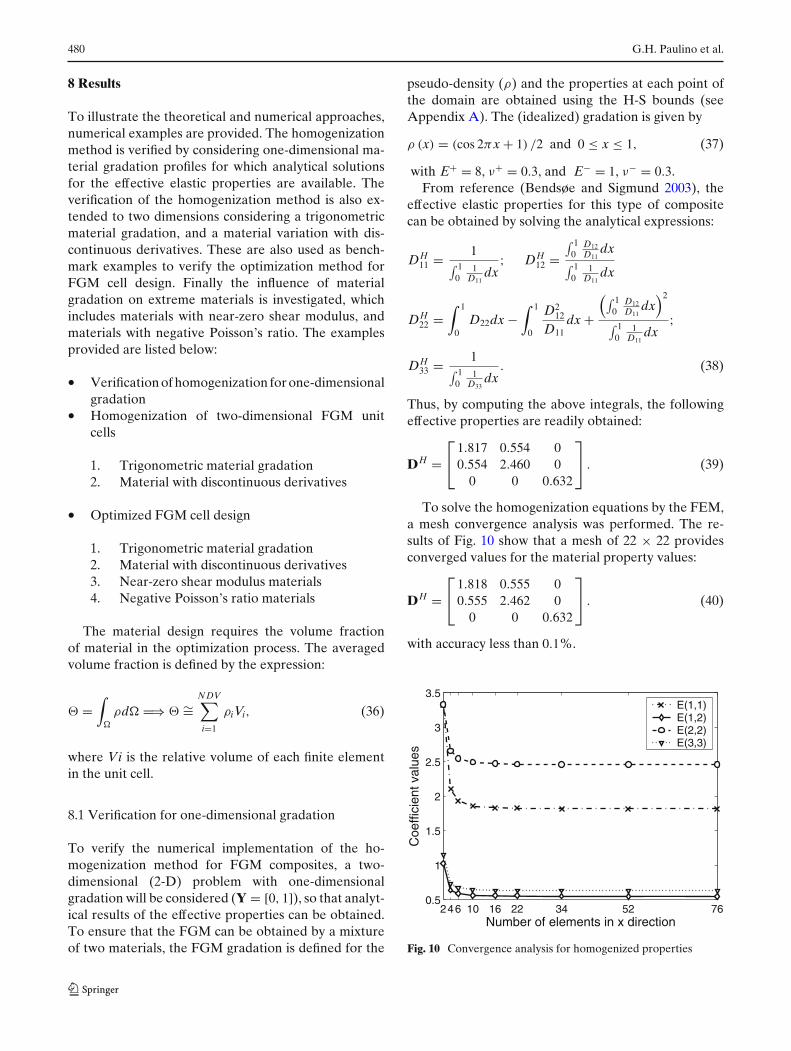
To solve the homogenization equations by the FEM,a mesh convergence analysis was performed. The re-sults of Fig. 10 show that a mesh of 22 × 22 providesconverged values for the material property values:

DH =⎡

⎣1.818 0.555 00.555 2.462 0

0 0 0.632

⎤

⎦ . (40)

with accuracy less than 0.1%.

246 10 16 22 34 52 760.5

1

1.5

2

2.5

3

3.5

Number of elements in x direction

Coe

ffici

ent v

alue

s

E(1,1)E(1,2)E(2,2)E(3,3)

Fig. 10 Convergence analysis for homogenized properties


Fig. 11 a Trigonometric material gradation; b material with discontinuous derivatives

8.2 Homogenization of FGM unit cells

To illustrate the potentiality of the method, some two-dimensional (2-D) FGM composite unit cells (Y =[0, 1] × [0, 1]) with two-dimensional gradation were ho-mogenized. The same homogenized properties wereused as input for the material design problem inSection 4 to check its capability to recover the materialdistribution.

8.2.1 Example 1 – trigonometric material gradation

The first gradation law considered (for the pseudo-density) is given by:

ρ (x, y) = (sin 2πx sin 2πy + 1) /2 and

0 ≤ x ≤ 1; 0 ≤ y ≤ 1. (41)

as shown in Fig. 11a.

(a) (b)

Fig. 12 Benchmark material with trigonometric gradation.a Pseudo-density distribution in the unit cell; b correspondingcomposite material matrix

Figure 12a and b describe the pseudo-density distri-bution in the unit cell and the corresponding compositematerial matrix. The calculated effective property val-ues using a 40 × 40 mesh are

DH =⎡

⎣2.7148 0.9180 00.9180 2.7148 0

0 0 1.0266

⎤

⎦ . (42)

8.2.2 Example 2—material with discontinuousderivatives

The second gradation law considered (for the pseudo-density) is given by:

ρ (x, y) =

⎧⎪⎪⎨

⎪⎪⎩

1 − 2x and 0 ≤ x ≤ 1/2; x ≤ y ≤ 1 − x2x − 1 and 1/2 ≤ x ≤ 1; 1 − x ≤ y ≤ x1 − 2y and 0 ≤ y ≤ 1/2; y ≤ x ≤ 1 − y2y − 1 and 1/2 ≤ y ≤ 1; 1 − y ≤ x ≤ y

.

(43)

as shown in Fig. 11b.Notice that this gradation does not have continuous

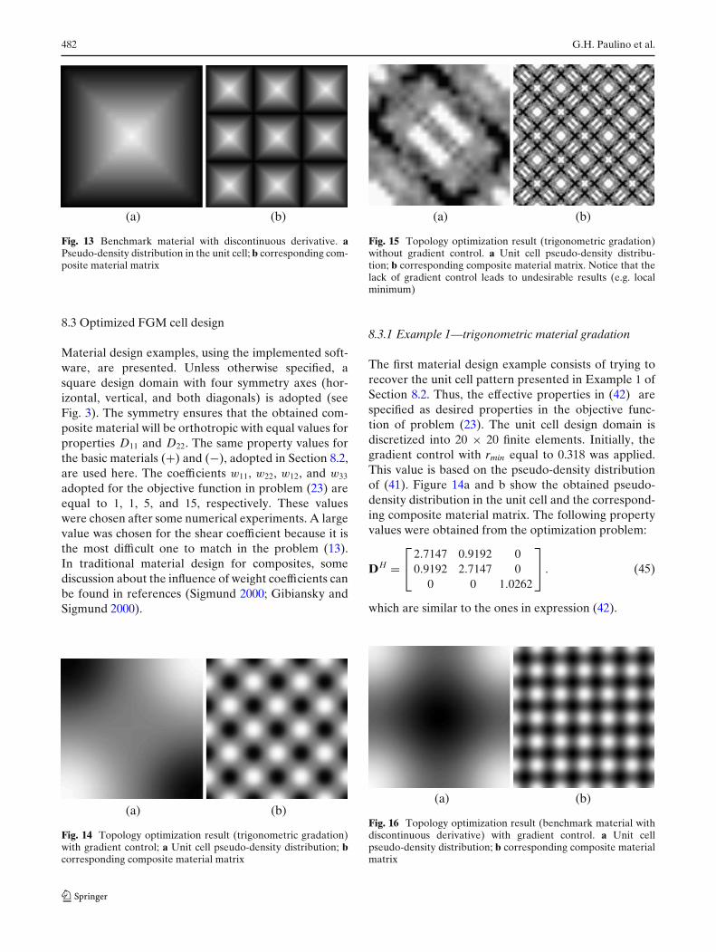
derivatives. Figure 13a and b describe the pseudo-density distribution in the unit cell and the correspond-ing composite material matrix. The calculated effectiveproperty values using a 40 × 40 mesh are

DH =⎡

⎣4.0457 1.1507 01.1507 4.0457 0

0 0 1.2954

⎤

⎦ . (44)


(a) (b)

Fig. 13 Benchmark material with discontinuous derivative. aPseudo-density distribution in the unit cell; b corresponding com-posite material matrix

8.3 Optimized FGM cell design

Material design examples, using the implemented soft-ware, are presented. Unless otherwise specified, asquare design domain with four symmetry axes (hor-izontal, vertical, and both diagonals) is adopted (seeFig. 3). The symmetry ensures that the obtained com-posite material will be orthotropic with equal values forproperties D11 and D22. The same property values forthe basic materials (+) and (−), adopted in Section 8.2,are used here. The coefficients w11, w22, w12, and w33

adopted for the objective function in problem (23) areequal to 1, 1, 5, and 15, respectively. These valueswere chosen after some numerical experiments. A largevalue was chosen for the shear coefficient because it isthe most difficult one to match in the problem (13).In traditional material design for composites, somediscussion about the influence of weight coefficients canbe found in references (Sigmund 2000; Gibiansky andSigmund 2000).

(a) (b)

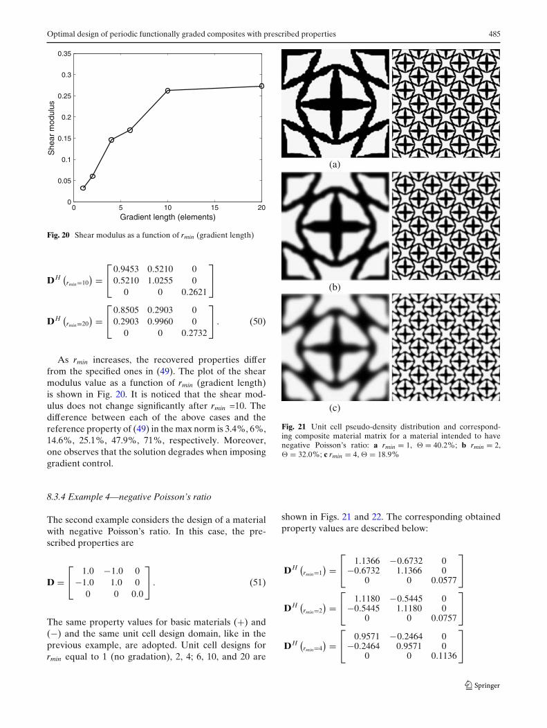
Fig. 14 Topology optimization result (trigonometric gradation)with gradient control; a Unit cell pseudo-density distribution; bcorresponding composite material matrix

(a) (b)

Fig. 15 Topology optimization result (trigonometric gradation)without gradient control. a Unit cell pseudo-density distribu-tion; b corresponding composite material matrix. Notice that thelack of gradient control leads to undesirable results (e.g. localminimum)

8.3.1 Example 1—trigonometric material gradation

The first material design example consists of trying torecover the unit cell pattern presented in Example 1 ofSection 8.2. Thus, the effective properties in (42) arespecified as desired properties in the objective func-tion of problem (23). The unit cell design domain isdiscretized into 20 × 20 finite elements. Initially, thegradient control with rmin equal to 0.318 was applied.This value is based on the pseudo-density distributionof (41). Figure 14a and b show the obtained pseudo-density distribution in the unit cell and the correspond-ing composite material matrix. The following propertyvalues were obtained from the optimization problem:

DH =⎡

⎣2.7147 0.9192 00.9192 2.7147 0

0 0 1.0262

⎤

⎦ . (45)

which are similar to the ones in expression (42).

(a) (b)

Fig. 16 Topology optimization result (benchmark material withdiscontinuous derivative) with gradient control. a Unit cellpseudo-density distribution; b corresponding composite materialmatrix


Notice that the recovered pattern shown in Fig. 14bis similar to the original one shown in Fig. 12b. Quanti-tavely, the averaged volume fraction () of the recov-ered pattern for material (+) is equal to 0.5, exactly thesame value for the original pattern.

If no gradient control is used, the results shown inFigs. 15a and b are obtained, which are different fromthe original pattern shown in Fig. 12a and b, and thefollowing property values are obtained:

DH =⎡

⎣2.7147 0.9173 00.9173 2.7147 0

0 0 1.0267

⎤

⎦ . (46)

These results are similar to the ones in expressions(42) and (45). However, in this case, the averagedvolume fraction of the recovered pattern is equal to0.483, which is different from the original pattern. Thisexample shows that the use of gradient control is quitesignificant for designing FGM microstructures.

8.3.2 Example 2—material with discontinuousderivatives

This example consists of recovering the unit cell pat-tern of Example 2 presented in Section 8.2. Thus, theeffective properties in (44) are specified as desiredproperties in the objective function of problem (23).The same design domain as the previous example isadopted.

Initially, the gradient control with rmin equal to 0.5was applied. Figure 16a and b show the pseudo-density

(a) (b)

Fig. 17 Topology optimization result (benchmark mate-rial with discontinuous derivative) without gradient control.a Unit cell pseudo-density distribution; b corresponding compos-ite material matrix. Again, the lack of gradient control leads toundesirable results (e.g. local minimum)

distribution in the unit cell and the corresponding com-posite material matrix. The following properties wereobtained from the optimization problem:

DH =⎡

⎣3.9669 1.1735 01.1735 3.9669 0

0 0 1.3204

⎤

⎦ . (47)

which are similar to the ones in expression (44).In the original pattern, the material gradation deriv-

atives are not continuous. Thus, by using gradient con-trol we cannot expect to recover the same pattern asshown in Fig. 13a and b. However, the method pro-vides the best solution close to the desired one in theminimum square sense. Quantitatively, the averaged

(a)

(b)

(c)

Fig. 18 Unit cell pseudo-density distribution and correspond-ing composite material matrix for a material with near zeroshear modulus: a rmin = 1 , = 43.4%; b rmin = 2, = 36.1%;c rmin = 4, = 25.4%


volume fraction of the recovered pattern for material(+) is equal to 0.658, while for the original pattern is0.666.

If no gradient control is used, the results in Fig. 17aand b are obtained, which are different from the origi-nal pattern shown in Fig. 13a and b, however, it recov-ers the property values ( (44) and (47)):

DH =⎡

⎣4.045 1.1510 0

1.1510 4.045 00 0 1.2951

⎤

⎦ . (48)

The average volume fraction of the recovered pattern isequal to 0.649, which is different from the original pat-tern (0.666). As expected, the FGM gradation imposes

(a)

(b)

(c)

Fig. 19 Unit cell pseudo-density distribution and correspond-ing composite material matrix for a material with near zeroshear modulus: a rmin = 6, = 19.5%; b rmin = 10, = 11.3%;c rmin = 20, = 13.4%

additional constraints in the material design process,which means that not all property values that could befeasible in a unit cell design without this constraint, canbe obtained.

8.3.3 Example 3—near zero shear modulus

The objective of this example is to analyze the influenceof FGM gradation in the design of extreme materials. Itis known that extreme materials can only be obtainedwith solid-void (0–1) designs and steep material varia-tion (Sigmund 2000). However, usually, some gradationis obtained in the manufacturing processes of suchmaterials. Thus, the question is how this gradation influ-ences the behavior of a designed extreme material. Toillustrate this point, we consider the design of materialswith zero shear modulus and negative Poisson’s ratio.First, the design of a material with zero shear modulusis considered.

Such material consists essentially of a mechanism,thus in the case of material design there will be always aminimum value for the shear modulus. The prescribedproperties are

D =⎡

⎣1.0 1.0 01.0 1.0 00 0 0.0

⎤

⎦ . (49)

In this problem, Young’s modulus, E+ and E−, andPoisson’s ratio, ν+ and ν−, of basic materials are equalto 27.3, 0.0, 0.3, and 0.0, respectively. The unit cell de-sign domain is discretized into 40 × 40 finite elements.The unit cell designs for rmin equal to 1 (no gradation),2, 4; 6, 10, and 20 are shown in Figs. 18 and 19. Thecorresponding computed property values are describedbelow:

DH (rmin=1

) =⎡

⎣1.0356 0.9662 00.9662 1.0356 0

0 0 0.0324

⎤

⎦

DH (rmin=2

) =⎡

⎣1.0549 0.9412 00.9412 1.0549 0

0 0 0.0602

⎤

⎦

DH (rmin=4

) =⎡

⎣1.0064 0.8593 00.8593 1.0064 0

0 0 0.1463

⎤

⎦

DH (rmin=6

) =⎡

⎣1.0357 0.7493 00.7493 1.0357 0

0 0 0.1688

⎤

⎦


0 5 10 15 200

0.05

0.1

0.15

0.2

0.25

0.3

0.35

Gradient length (elements)

She

ar m

odul

us

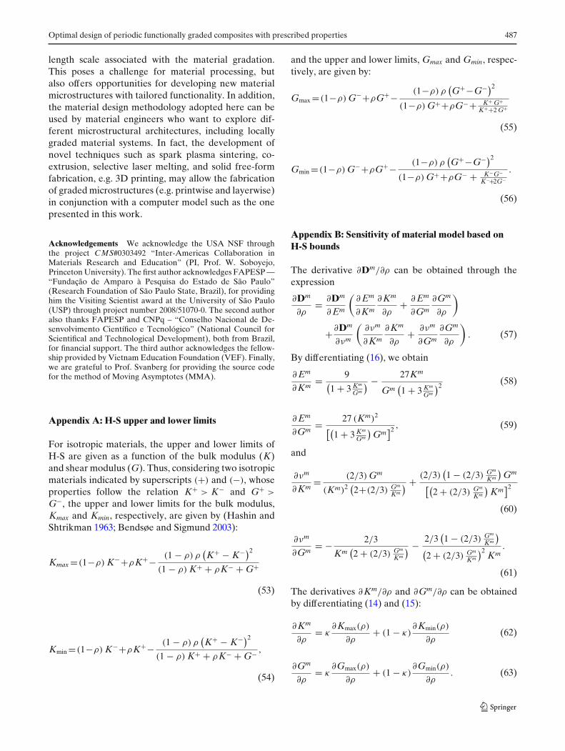
Fig. 20 Shear modulus as a function of rmin (gradient length)

DH (rmin=10

) =⎡

⎣0.9453 0.5210 00.5210 1.0255 0

0 0 0.2621

⎤

⎦

DH (rmin=20

) =⎡

⎣0.8505 0.2903 00.2903 0.9960 0

0 0 0.2732

⎤

⎦ . (50)

As rmin increases, the recovered properties differfrom the specified ones in (49). The plot of the shearmodulus value as a function of rmin (gradient length)is shown in Fig. 20. It is noticed that the shear mod-ulus does not change significantly after rmin =10. Thedifference between each of the above cases and thereference property of (49) in the max norm is 3.4%, 6%,14.6%, 25.1%, 47.9%, 71%, respectively. Moreover,one observes that the solution degrades when imposinggradient control.

8.3.4 Example 4—negative Poisson’s ratio

The second example considers the design of a materialwith negative Poisson’s ratio. In this case, the pre-scribed properties are

D =⎡

⎣1.0 −1.0 0

−1.0 1.0 00 0 0.0

⎤

⎦ . (51)

The same property values for basic materials (+) and(−) and the same unit cell design domain, like in theprevious example, are adopted. Unit cell designs forrmin equal to 1 (no gradation), 2, 4; 6, 10, and 20 are

(a)

(b)

(c)

Fig. 21 Unit cell pseudo-density distribution and correspond-ing composite material matrix for a material intended to havenegative Poisson’s ratio: a rmin = 1, = 40.2%; b rmin = 2, = 32.0%; c rmin = 4, = 18.9%

shown in Figs. 21 and 22. The corresponding obtainedproperty values are described below:

DH (rmin=1

) =⎡

⎣1.1366 −0.6732 0

−0.6732 1.1366 00 0 0.0577

⎤

⎦

DH (rmin=2

) =⎡

⎣1.1180 −0.5445 0

−0.5445 1.1180 00 0 0.0757

⎤

⎦

DH (rmin=4

) =⎡

⎣0.9571 −0.2464 0

−0.2464 0.9571 00 0 0.1136

⎤

⎦


(a)

(b)

(c)

Fig. 22 Unit cell pseudo-density distribution and correspondingcomposite material matrix for a material intended to have nega-tive Poisson’s ratio: a rmin = 6, = 8.8%; b rmin = 10, = 4.3%;c rmin = 20, = 10.3%

DH (rmin=6

) =⎡

⎣0.7399 − 0.0408 0

−0.0408 0.7399 00 0 0.1141

⎤

⎦

DH (rmin=10

) =⎡

⎣0.4792 0.0363 00.0363 0.4792 0

0 0 0.0553

⎤

⎦

DH (rmin=20

) =⎡

⎣0.2830 0.0467 00.0467 0.2830 0

0 0 0.0624

⎤

⎦ . (52)

For the 0–1 problem a Poisson’s ratio close to −1could not be obtained. The reason is that the methoddid not allow for flexible hinges, thus, the lower valuefor the Poisson’s ratio that could be obtained was−0.6732 . The plot of the Poisson’s ratio value as a func-

0 5 10 15 20-0.7

-0.6

-0.5

-0.4

-0.3

-0.2

-0.1

0

0.1

Gradient length (elements)

Poi

son'

s ra

tio

Fig. 23 Poisson’s ratio as a function of rmin (gradient length)

tion of rmin (gradient length) is shown in Fig. 23. Like inthe previous example, it is noticed that the Poisson’sratio value does not change significantly after rmin =10.The difference between each of the above cases and thereference property of (51) in the max norm is 32.7%,45.6%, 75.4%, 95.9%, 103.6%, 104.7%, respectively. Asin the previous section, one observes that the solutiondegrades when imposing gradient control. Moreover, atthe end (largermin), the Poisson’s ratio is not negative.

9 Conclusions

This work shows that the material design method basedon the continuum topology optimization together witha gradient control technique is applicable to the de-sign of FGM microstructures. The continuous materialdistribution leads to a natural representation of thechange of material properties inside the design domainin a continuous fashion, which is closely related to theFGM concept. The gradient control introduces a lengthscale in the process, which allows local control of theFGM gradation, and thus leads to feasible results. Asexpected, in the case of extreme materials, the presenceof gradation moves the property values far from theextreme material property values. After a certain gra-dation control magnitude, the material behavior doesnot seem to be affected significantly.

The present work offers room for further exten-sions such as exploring graded three-dimensional archi-tectures. Moreover, as indicated in the introduction,the present simulation framework can be used inconjunction with manufacturing techniques to achievecomposites with locally graded microstructures. Wenotice that the resulting architecture has an additional


length scale associated with the material gradation.This poses a challenge for material processing, butalso offers opportunities for developing new materialmicrostructures with tailored functionality. In addition,the material design methodology adopted here can beused by material engineers who want to explore dif-ferent microstructural architectures, including locallygraded material systems. In fact, the development ofnovel techniques such as spark plasma sintering, co-extrusion, selective laser melting, and solid free-formfabrication, e.g. 3D printing, may allow the fabricationof graded microstructures (e.g. printwise and layerwise)in conjunction with a computer model such as the onepresented in this work.

Acknowledgements We acknowledge the USA NSF throughthe project CMS#0303492 “Inter-Americas Collaboration inMaterials Research and Education” (PI, Prof. W. Soboyejo,Princeton University). The first author acknowledges FAPESP —“Fundação de Amparo à Pesquisa do Estado de São Paulo”(Research Foundation of São Paulo State, Brazil), for providinghim the Visiting Scientist award at the University of São Paulo(USP) through project number 2008/51070-0. The second authoralso thanks FAPESP and CNPq – “Conselho Nacional de De-senvolvimento Científico e Tecnológico” (National Council forScientifical and Technological Development), both from Brazil,for financial support. The third author acknowledges the fellow-ship provided by Vietnam Education Foundation (VEF). Finally,we are grateful to Prof. Svanberg for providing the source codefor the method of Moving Asymptotes (MMA).

Appendix A: H-S upper and lower limits

For isotropic materials, the upper and lower limits ofH-S are given as a function of the bulk modulus (K)and shear modulus (G). Thus, considering two isotropicmaterials indicated by superscripts (+) and (−), whoseproperties follow the relation K+ > K− and G+ >

G−, the upper and lower limits for the bulk modulus,Kmax and Kmin, respectively, are given by (Hashin andShtrikman 1963; Bendsøe and Sigmund 2003):

Kmax =(1−ρ) K−+ρK+− (1 − ρ) ρ(K+ − K−)2

(1 − ρ) K+ + ρK− + G+

(53)

Kmin =(1−ρ) K−+ρK+− (1 − ρ) ρ(K+ − K−)2

(1 − ρ) K+ + ρK− + G− ,

(54)

and the upper and lower limits, Gmax and Gmin, respec-tively, are given by:

Gmax =(1−ρ) G−+ρG+− (1−ρ) ρ(G+−G−)2

(1−ρ) G++ρG−+ K+ G+K++2 G+

(55)

Gmin =(1−ρ) G−+ρG+− (1−ρ) ρ(G+−G−)2

(1−ρ) G++ρG− + K−G−K−+2G−

.

(56)

Appendix B: Sensitivity of material model based onH-S bounds

The derivative ∂Dm/∂ρ can be obtained through theexpression

∂Dm

∂ρ= ∂Dm

∂ Em

(∂ Em

∂Km

∂Km

∂ρ+ ∂ Em

∂Gm

∂Gm

∂ρ

)

+∂Dm

∂νm

(∂νm

∂Km

∂Km

∂ρ+ ∂νm

∂Gm

∂Gm

∂ρ

). (57)

By differentiating (16), we obtain

∂ Em

∂Km= 9

(1 + 3 Km

Gm

) − 27Km

Gm(1 + 3 Km

Gm

)2 (58)

∂ Em

∂Gm= 27 (Km)2

[(1 + 3 Km

Gm

)Gm

]2 , (59)

and

∂νm

∂Km= (2/3) Gm

(Km)2 (2+(2/3) Gm

Km

) + (2/3)(1 − (2/3) Gm

Km

)Gm

[(2 + (2/3) Gm

Km

)Km

]2

(60)

∂νm

∂Gm= − 2/3

Km(2 + (2/3) Gm

Km

) − 2/3(1 − (2/3) Gm

Km

)

(2 + (2/3) Gm

Km

)2Km

.

(61)

The derivatives ∂Km/∂ρ and ∂Gm/∂ρ can be obtainedby differentiating (14) and (15):

∂Km

∂ρ= κ

∂Kmax(ρ)

∂ρ+ (1 − κ)

∂Kmin(ρ)

∂ρ(62)

∂Gm

∂ρ= κ

∂Gmax(ρ)

∂ρ+ (1 − κ)

∂Gmin(ρ)

∂ρ. (63)


Finally, considering Kmax(ρ), Kmin(ρ), Gmax(ρ), andGmin(ρ) given by (53), (54), (55), and (56), we obtain

∂Kmax

∂ρ= −K− + K+ + ρ

(K+ − K−)2

(1 − ρ) K+ + ρK− + G+

− (1 − ρ)(K+ − K−)2

(1 − ρ) K+ + ρK− + G+

+ (1 − ρ) ρ(K+ − K−)2 (

K− − K+)

((1 − ρ) K+ + ρK− + G+)2 (64)

∂Kmin

∂ρ= −K− + K+ + ρ

(K+ − K−)2

(1 − ρ) K+ + ρK− + G−

− (1 − ρ)(K+ − K−)2

(1 − ρ) K+ + ρK− + G−

+ (1 − ρ) ρ(K+ − K−)2 (

K− − K+)

((1 − ρ) K+ + ρK− + G−)2 (65)

∂Gmax

∂ρ= −G− + G+ + ρ

(G+ − G−)2

(1 − ρ) G+ + ρG− + K+G+K++2G+

− (1 − ρ)(G+ − G−)2

(1 − ρ) G+ + ρG− + K+G+K++2G+

+ (1 − ρ) ρ(G+ − G−)2 (

G− − G+)

((1 − ρ) G+ + ρG− + K+G+

K++2G+)2 (66)

∂Gmin

∂ρ= −G− + G+ + ρ

(G+ − G−)2

(1 − ρ) G+ + ρG− + K−G−K−+2G−

− (1 − ρ)(G+ − G−)2

(1 − ρ) G+ + ρG− + K−G−K−+2G−

+ (1 − ρ) ρ(G+ − G−)2 (

G− − G+)

((1 − ρ) G+ + ρG− + K−G−

K−+2G−)2 . (67)

Thus, the sensitivity for the material model based onthe H-S bounds can be obtained.

References

Allaire G (2002) Shape optimization by the homogenizationmethod. Applied mathematical sciences, vol 146. ISBN-10:0387952985. Springer, New York

Bendsøe MP, Kikuchi N (1988) Generating optimal topologies instructural design using a homogenization method. ComputMethods Appl Mech Eng 71(2):197–224

Bendsøe MP, Sigmund O (2003) Topology optimization: theory,methods and application. Springer, Berlin

Bruyneel M, Duysinx P, Fleury C (2002) A family of MMAapproximations for structural optimization. Struct MultidiscOptim 24(4):263–276

Carbonari RC, Silva ECN, Paulino GH (2007) Topology opti-mization design of functionally graded bimorph-type piezo-electric actuators. Smart Mater Struct 16(6):2605–2620

Chen BC, Silva ECN, Kikuchi N (2001) Advances in computa-tional design and optimization with application to MEMS.Int J Numer Methods Eng 52(1–2):23–62

Cherkaev A (2000) Variational methods for structural opti-mization. Applied mathematical sciences, vol 140. ISBN-10:0387984623. Springer, New York

Cherkaev A, Gibiansky LV (1993) Coupled estimates for thebulk and shear moduli of a 2-dimensional isotropic elasticcomposite. J Mech Phys Solids 41(5):937–980

Cherkaev A, Gibiansky LV (1996) Extremal structures of mul-tiphase heat conducting composites. Int J Solids Struct33(18):2609–2623

Cherkaev A, Kohn R (1997) Topics in the mathematicalmodelling of composite materials. ISBN-10: 3764336625.Birkhauser, Boston

Cox SJ, Dobson DC (1999) Maximizing band gaps intwo-dimensional photonic crystals. SIAM J Appl Math59(6):2108–2120

Cox SJ, Dobson DC (2000) Band structure optimization of two-dimensional photonic crystals in H-polarization. J ComputPhys 158(2):214–224

Crumm AT, Halloran JW (1998) Fabrication of microconfiguredmulticomponent ceramics. J Am Ceram Soc 81(4):1053–1057

Crumm AT, Halloran JW, Silva ECN, de Espinosa FM (2007)Microconfigured piezoelectric artificial materials for hy-drophones. J Mater Sci 42(11):3944–3950

Diaz AR, Benard A (2003) Designing materials with prescribedelastic properties using polygonal cells. Int J Numer MethodsEng 57(3):301–314

Gibiansky LV, Sigmund O (2000) Multiphase composites withextremal bulk modulus. J Mech Phys Solids 48(3):461–498

Gibiansky LV, Torquato S (1995) Rigorous link between the con-ductivity and elastic-moduli of fiber-reinforced composite-materials. Philos Trans R Soc Lond Ser A Math Phys Sci353(1702):243–278

Gibiansky LV, Torquato S (1999) Matrix laminate composites:realizable approximations for the effective moduli of piezo-electric dispersions. J Mater Res 14(1):49–63

Guedes JM, Kikuchi N (1990) Preprocessing and postprocess-ing for materials based on the homogenization method withadaptive finite-element methods. Comput Methods ApplMech Eng 83(2):143–198

Guedes JM, Rodrigues HC, Bendsøe MP (2003) A material op-timization model to approximate energy bounds for cellu-lar materials under multiload conditions. Struct MultidiscOptim 25(5–6):446–452

Guest JK, Prévost JH, Belytschko T (2004) Achieving minimumlength scale in topology optimization using nodal designvariables and projection functions. Int J Numer MethodsEng 61:238–254

Hashin Z, Shtrikman S (1963) A variational approach of thetheory of elastic behavior of multiphase materials. J MechPhys Solids 11:127–140

Kim JH, Paulino GH (2002) Isoparametric graded finite elementsfor nonhomogeneous isotropic and orthotropic materials.ASME J Appl Mech 69(4):502–514

Kohn RV, Strang G (1986a) Optimal design and relaxationof variational problems, part I. Commun Pure Appl Math39(1):113–137


Kohn RV, Strang G (1986b) Optimal design and relaxation ofvariational problems, part II. Commun Pure Appl Math39(2):139–182

Kohn RV, Strang G (1986c) Optimal design and relaxation ofvariational problems, part III. Commun Pure Appl Math39(3):353–377

Larsen UD, Sigmund O, Bouwstra S (1997) Design and fabri-cation of compliant micromechanisms and structures withnegative Poisson’s ratio. J Microelectromechanical Syst 6(2):99–106

Lipton R, Northrup J (1994) Optimal bounds on the inplaneshear moduli for orthotropic elastic composites. SIAM JAppl Math 54(2):428–442

Matsui K, Terada K (2004) Continuous approximation of ma-terial distribution for topology optimization. Int J NumerMethods Eng 59:1925–1944

Mazumder J, Schifferer A, Choi J (1999) Direct materials depo-sition: designed macro and microstructure. Mater Res Innov3(3):118–131

Mazumder J, Dutta D, Kikuchi N, Ghosh A (2000) Closed loopdirect metal deposition: art to part. Opt Lasers Eng 34(4–6):397–414

Milton GW, Cherkaev AV (1995) Which elasticity tensors are rea-lizable? J Eng Mater Technol Trans ASME 117(4): 483–493

Miyamoto Y, Kaysser WA, Rabin BH, Kawasaki A, Ford RG(1999) Functionally graded materials: design, processing andapplications. Kluwer Academic, Dordrecht

Murat F, Tartar L (1985) Optimality conditions and homogeniza-tion. In: Mario A, Modica L, Spagnolo S (eds) Nonlinearvariational problems. Pitman, Boston, pp 1–8

Neves MM, Rodrigues H, Guedes JM (2000) Optimal designof periodic linear elastic microstructures. Comput Struct 76(1–3):421–429

Neves MM, Sigmund O, Bendsøe MP (2002) Topology opti-mization of periodic microstructures with a penalization ofhighly localized buckling modes. Int J Numer Methods Eng54(6):809–834

Paulino GH, Jin Z-H, Dodds Jr RH (2003) Failure of functionallygraded materials. In: Karihaloo B, Knauss WG (eds) Com-prehensive structural integrity, vol 2, chapter 13. ElsevierScience, Oxford, pp 607–644

Paulino GH, Silva ECN (2005) Design of functionally gradedstructures using topology optimization. Mat Sci Forum 492–493:435–440

Pindera M-J, Aboudi J, Arnold SM (1995) Limitations of theuncoupled, RVE-based micromechanical approach in theanalysis of functionally graded composites. Mech Mater20(1):77–94

Qi H, Kikuchi N, Mazumder J (2004) Interface study and bound-ary smoothing on designed composite material microstruc-tures for manufacturing purposes. Struct Multidisc Optim26(5):326–332

Qi J, Halloran JW (2004) Negative thermal expansion artificialmaterial from iron-nickel alloys by oxide co-extrusion withreductive sintering. J Mater Sci 39(13):4113–4118

Rahmatalla S, Swan CC (2003) Form finding of sparse structureswith continuum topology optimization. ASCE J Struct Eng129(12):1707–1716

Rahmatalla SF, Swan CC (2004) A Q4/Q4 continuum topol-ogy optimization implementation. Struct Multidisc Optim27:130–135

Reiter T, Dvorak GJ, Tvergaard V (1997) Micromechanical mod-els for graded composite materials. J Mech Phys Solids45(8):1281–1302

Sanchez-Palencia E (1980) Non-homogeneous media and vibra-tion theory. Lectures notes in physics 127. Springer, Berlin

Sigmund O (1994) Materials with prescribed constitutiveparameters—an inverse homogenization problem. Int JSolids Struct 31(17):2313–2329

Sigmund O (1995) Tailoring materials with prescribed elasticproperties. Mech Mater 20(4):351–368

Sigmund O (2000) A new class of extremal composites. J MechPhys Solids 48(2):397–428

Sigmund O, Jensen JS (2003) Systematic design of phononicband-gap materials and structures by topology optimiza-tion. Philos Trans R Soc Lond Ser A Math Phys Sci361(1806):1001–1019

Sigmund O, Torquato S (1996) Composites with extremalthermal expansion coefficients. Appl Phys Lett 69(21):3203–3205

Sigmund O, Torquato S (1997) Design of materials withextreme thermal expansion using a three-phase topologyoptimization method. J Mech Phys Solids 45(6):1037–1067

Sigmund O, Torquato S (1999) Design of smart compositematerials using topology optimization. Smart Mater Struc8(3):365–379

Sigmund O, Torquato S, Aksay IA (1998) On the design of 1–3piezocomposites using topology optimization. J Mater Res13(4):1038–1048

Silva ECN, Fonseca JSO, Kikuchi N (1998) Optimal design ofperiodic piezocomposites. Comput Methods Appl Mech Eng159(1–2):49–77

Silva ECN, Fonseca JSO, de Espinosa FM, Crumm AT, BradyGA, Halloran JW, Kikuchi N (1999a) Design of piezocom-posite materials and piezoelectric transducers using topol-ogy optimization - Part I. Arch Comput Methods Eng 6(2):117–182

Silva ECN, Nishiwaki S, Fonseca JSO, Kikuchi N (1999b)Optimization methods applied to material and flex-tensional actuator design using the homogenizationmethod. Comput Methods Appl Mech Eng 172(1–4):241–271

Silva ECN, Paulino GH (2004) Topology optimization applied tothe design of functionally graded material (FGM) structures.In: Proceedings of 21st international congress of theoreticaland applied mechanics (ICTAM) 2004, 15–21 August 2004,Warsaw

Smith WA (1992) Limits to the enhancement of piezoelectrictransducers achievable by materials engineering. Proc IEEEUltrason Symp 1:697–702

Suresh S, Mortensen A (1988) Fundamentals of functionallygraded materials. IOM Communications, London

Svanberg K (1987) The method of moving asymptotes—a newmethod for structural optimization. Int J Numer MethodsEng 24:359–373

Torquato S (2002) Random heterogeneous materials—microstructure and macroscopic properties. ISBN-10:0387951679. Springer, New York

Torquato S, Hyun S, Donev A (2003) Optimal design of manufac-turable three-dimensional composites with multifunctionalcharacteristics. J Appl Phys 94(9):5748–5755

Van Hoy C, Barda A, Griffith M, Halloran JW (1998) Micro-fabrication of ceramics by co-extrusion. J Am Ceram Soc81(1):152–158

Yin HM, Sun LZ, Paulino GH (2004) Micromechanics-basedelastic model for functionally graded materials with particleinteractions. Acta Mater 52(12):3535–3543

optimal design of periodic functionally graded composites

Documents