optimal design solutions of concrete bridges …1293043/fulltext01.pdfoptimal design solutions of...
TRANSCRIPT

Optimal design solutions of concrete bridges considering
environmental impact and investment cost
ELISA KHOURI CHALOUHI
Licentiate Thesis Stockholm, Sweden 2019

TRITA-ABE-DLT-194 ISBN 978-91-7873-114-5
KTH School of ABE SE-100 44 Stockholm
Sweden
Akademisk avhandling som med tillstånd av KTH i Stockholm framlägges till offentlig granskning för avläggande av teknisk licentiatexamen i brobyggnad fredagen den 22 mars 2019 klockan 13:00 i sal M108, KTH, Brinellvägen 23, Stockholm. Avhandlingen försvaras på engelska. © Elisa Khouri Chalouhi, March 2019 Tryck: Universitetsservice US-AB
iii
Abstract
The most used design approach for civil engineering structures is a trial and error procedure; the designer chooses an initial configuration, tests it and changes it until all safety requirements are met with good material utilization. Such a procedure is time consuming and eventually leads to a feasible solution, while several better ones could be found. Indeed, together with safety, environmental impact and investment cost should be decisive factors for the selection of structural solutions. Thus, structural optimization with respect to environmental impact and cost has been the subject of many researches in the last decades. However, design techniques based on optimization haven’t replaced the traditional design procedure yet. One of the reasons might be the constructive feasibility of the optimal solution. Moreover, concerning reinforced concrete beam bridges, to the best of the author knowledge, no study in the literature has been published dealing with the optimization of the entire bridge including both the structural configuration and cross-section dimensions. In this thesis, a two-steps automatic design and optimization procedure for reinforced concrete road beam bridges is presented. The optimization procedure finds the solution that minimizes the investment cost and the environmental impact of the bridge, while fulfilling all requirements of Eurocodes. In the first step, given the soil morphology and the two points to connect, it selects the optimal number of spans, type of piers-deck connections and piers location taking into account any obstacle the bridge has to cross. In the second and final step, it finds the optimal dimensions of the deck cross-section and produces the detailed reinforcement design. Constructability is considered and quantified within the investment cost to avoid a merely theoretical optimization. The well-known Genetic Algorithm (GA) and Pattern Search optimization algorithms have been used. However, to reduce the computational effort and make the procedure more user-friendly, a memory system has been integrated and a modified version of GA has been developed. Moreover, the design and optimization procedure is

iv
used to study the relationship between the optimal solutions concerning investment cost and environmental impact. One case study concerning the re-design of an existing road bridge is presented. Potential savings obtained using the proposed method instead of the classic design procedure are presented. Finally, parametric studies on the total bridge length have been carried out and guidelines for designers have been produced regarding the optimal number of spans.
Keywords: Structural optimization; Automated design; Beam bridges; Environmental impact; Investment cost
v
Sammanfattning
Den mest använda designmetoden för konstruktioner är ett s.k. ”trial and error” förfarande; konstruktören väljer en grundkonfiguration, testar den och ändrar det till dess alla säkerhetskrav är uppfyllda. Ett sådant förfarande är tidsödande men leder så småningom till en genomförbar lösning, dock kan flera bättre lösningar existera. Det är en självklarhet att säkerhet, miljöpåverkan och investeringskostnad ska vara avgörande faktorer för val av strukturella lösningar. Strukturell optimering med avseende på miljöpåverkan och kostnad har således varit föremål för många undersökningar under de senaste decennierna. Dock har tekniken som bygger på optimering inte ersatt det traditionella design förfarandet ännu. En av anledningarna till det kan vara byggbarhet av den optimerade lösningen. Dessutom har ingen studie gällande armerade betongbalkbroar som behandlar optimering av hela bron inklusive både strukturella konfigurationen och dimensioner hittats i litteraturstudien. I denna avhandling presenteras ett två-stegs automatiskt dimensioneringsförfarande för armerade betongbalkbroar för vägtrafik. Algoritmen beräknar fram den lösning som minimerar brons investeringskostnad och miljöpåverkan och samtidigt uppfyller samtliga krav i Eurokoderna. I det första steget, där markens beskaffenhet och anslutningspunkter beaktas, väljer algoritmen det optimala antalet spann, typ av lager och stödens läge med hänsyn till eventuella hinder under bron. I det andra och sista steget, hittar algoritmen de optimala dimensionerna av brofarbanan och producerar detaljutformningen och placering av armering. Byggbarheten beaktas och kvantifieras inom investeringskostnaden för att undvika suboptimala lösningar. De välkända optimeringsalgoritmerna ”Genetic Algorithm (GA)” och ”Pattern Search Algorithm” har använts. För att minska beräkningstiden och göra programmet mer användarvänligt, har en minnesfunktion integrerats och en modifierad version av GA har utvecklats. Den utvecklade algoritmen har också använts för att studera sambandet mellan optimala lösningar beträffande investeringskostnad och miljöpåverkan.

vi
En fallstudie av en befintlig vägbro presenteras. Potentiella besparingar som erhålls med den föreslagna metoden i stället för ett normalt dimensioneringsförfarande presenteras. Slutligen, har parametriska studier för olika brolängder genomförts och riktlinjer för konstruktörer presenterats för optimala antalet brospann.
Nyckelord: Strukturell optimering; Automatiserad dimensionering; Balkbroar; Miljöpåverkan; Investeringskostnad

vii
Preface
The research work presented in this thesis was carried out at the Department of Civil and Architectural Engineering, KTH Royal Institute of Technology, Stockholm. It has been appreciatively financed by the Swedish Transport Administration (Trafikverket) and ELU Konsult AB. I would like to express my most sincere gratitude towards my supervisors Professor Raid Karoumi and Professor Costin Pacoste for their guidance and continuous support. Special thanks go to Dr. Peter Simonsson for his time and his feedbacks and to Professor Jean-Marc Battini for taking the time to review this thesis. I would also like to thank my colleagues and friends at the Division of Structural Engineering and Bridges. Not only they shared their knowledge and experience with me, but they have always been there for a talk and a laugh. Sincere thanks go to my friends who are my second family. Finally and most importantly, thank to my amazing parents and my beloved brother for always believing in me and making me feel loved regardless of the physical distance.
Stockholm, March 2019 Elisa Khouri Chalouhi


ix
List of publications
Part of the work of this thesis resulted in a journal paper
Khouri Chalouhi, E., Pacoste, C. and Karoumi, R. Topological and size optimization of RC beam bridges: an automated design approach for cost effective and environmental friendly solutions. Submitted to Engineering Structures in December 2018.

xi
Contents
Abstract .............................................................................................................. iii
Sammanfattning .................................................................................................. v
Preface ............................................................................................................... vii
List of publications ............................................................................................ ix
Contents .............................................................................................................. xi
List of Abbreviations ........................................................................................ xv
1 Introduction ............................................................................................ 1
1.1 Background .................................................................................... 1
1.2 Aim and scope ................................................................................ 4
1.3 Outline of the thesis ....................................................................... 5
2 Optimization theory ............................................................................... 7
2.1 Design variables ............................................................................. 8
2.2 Objective functions ........................................................................ 8
2.3 Constraints ..................................................................................... 9
2.4 Optimization algorithms ............................................................... 10
3 Optimization of RC beam bridges ....................................................... 13
3.1 Design and optimization procedure .............................................. 13

CONTENTS
xii
3.2 Objective functions ....................................................................... 15
3.2.1 Investment cost ............................................................. 15
3.2.2 Environmental impact ................................................... 22
3.3 Constraints .................................................................................... 26
3.3.1 ULS and SLS ................................................................ 26
3.3.2 Infeasible regions for piers............................................ 30
3.3.3 Minimum vertical clearance ......................................... 30
3.3.4 Cross-section dimensions and span length .................... 31
3.4 Optimization algorithms ............................................................... 32
3.4.1 Genetic Algorithm ........................................................ 33
3.4.2 Pattern Search ............................................................... 36
4 Case study: Bridge over Norrtälje River ............................................ 39
4.1 The built structure ........................................................................ 39
4.2 Optimal solution: results and discussion ...................................... 40
4.2.1 Effect of the initial deck dimensions on the optimal static system ...................................................................................... 42
4.2.2 Optimal static system .................................................... 45
4.2.3 Optimal deck dimensions .............................................. 47
4.2.4 Effect of initial mesh size on the deck dimensions ....... 54
4.2.5 Effect of number of variables on the performance of the optimization .................................................................................. 62
4.2.6 Easy-to-build optimal solutions .................................... 66
4.2.7 Effect of reduced unit impacts of materials .................. 68
5 Parametric studies ................................................................................ 71
5.1 Optimal number of spans .............................................................. 71
5.2 Effect of material prices on the optimal number of spans ............ 74
5.3 Effect of unit emissions on the optimal number of spans ............. 76
6 Concluding remarks ............................................................................. 79

CONTENTS
xiii
6.1 Conclusions .................................................................................. 79
6.2 Further research ............................................................................ 81
Bibliography ...................................................................................................... 83

xv
List of Abbreviations
ABC
ANN
BOS
BS
CS
EI
EPSO
ESO
FB
FEM
GA
GFRP
HCS
Artificial bee colony
Artificial neural network
Buildable optimal solution
Built solution
Cross-section
Environmental impact
Enhanced particle swarm optimization
Evolutionary structural optimisation
Fixed bearing
Finite element method
Genetic algorithm
Glass fiber reinforced polymer
Hybrid cable-stayed suspension

LIST OF ABBREVIATIONS
xvi
IC
LC
LCA
LCC
LCI
LCIA
MB
MCBO
MC
OS
PC
PS
RC
SLS
SVM
ULS
Investment cost
Labour cost
Life cycle assessment
Life cycle cost
Life cycle inventory
Life cycle impact assessment
Movable bearing
Modified colliding bodies optimization
Material cost
Optimal solution
Prestressed concrete
Pattern search
Reinforced concrete
Serviceability limit state
Support vector machine
Ultimate limit state

1
1 Introduction
1.1 Background
The most used design approach for civil engineering structures is a trial and error procedure; the designer chooses an initial configuration for the structure, applies loads and check that all the safety requirements are met. Whenever they are not, the dimensions of the structure are changed until a feasible solution is found. Such a procedure has been used for decades in all engineering fields; however, besides being time consuming, it eventually leads to one feasible solution, while several better ones could exist. Indeed, safety is not the only requirement that the structure has to meet. The construction sector accounts for 39% of energy-related CO2 emissions (UN environment and International Energy Agency, 2017). In particular, concerning concrete structures, the cement industry by itself is responsible for around 5% of the global emissions of CO2 (Worrell, et al., 2001). Moreover, the economic burden of important infrastructures such as bridges is not negligible. Therefore, together with safety, environmental impact and investment cost should be decisive factors for the selection of structural solutions. The current design practice paired with years of experience can give rise to rules-of-thumbs for preliminary design (Paya-Zaforteza, et al., 2009) that could result in a good solution, but can’t guarantee the cost and emission-efficiency of the structure. To do so, several different solutions should be considered and compared in order to choose the optimal one. Thus, structural optimization with respect to environmental impact and cost has become of major interest in the last decades. Studies have been carried out on several types of civil engineering structures and different materials. Concerning
Chapter
1.1 BACKGROUND
2
buildings, Kaziolas et al. (2015), focused their work on minimizing the total life cost of timber buildings over a life span of 20 years. The environmental impact of concrete frames has been studied in several works by Paya-Zaforteza et al., who proposed a procedure for minimizing CO2 emissions and material cost simultaneously using simulated annealing (Paya-Zaforteza, et al., 2008). Camp & Huq (2013) tackled the same topic applying a hybrid form of a more recently developed algorithm: the big bang-big crunch algorithm (Erol & Eksin, 2006). Eleftheriadis et al. (2018) proposed a design and optimization approach based on BIM for the cost and CO2 optimization of reinforced concrete (RC) buildings. During the last decades, the bridge sector has been interested in structural optimization as well. Topology optimization has been applied in some studies to identify the best material layout for several types of bridges. Hong et al. (2003) applied the principal stress based evolutionary structural optimization (ESO) method to arch, cable-stayed and suspension bridges. Xie et al. (2018) optimized suspension, truss and shell bridges applying a bi-directional ESO technique. When the attention is focused on one particular bridge type, size optimization is a common area of research; some works consider also materials as design variables, while few works optimize the structural configuration. Concerning portal frame bridges, Perea et al. (2008) performed an economic optimization of road box frames with four different heuristic algorithms. Concrete type has been included as a variable together with the bridge dimensions. Yavari et al. (2017) performed the size optimization of RC slab frame bridges concerning environmental impact using Pattern Search. A case study is presented in this paper and the environmental-friendly solution is compared with the cost effective one obtained in a previous study (Yavari, et al., 2016). Regarding cable-stayed bridges, Hassan (2013) integrated FEM, B-spline curves and genetic algorithm to cost optimize the stay cables. Lee et al. (2008) considered asymmetric cable-stayed bridges under construction and applied the unit load method to cost optimize the prestressing force in the cables. Lute et al. (2009) used support vector machine (SVM) to reduce the computational time of the material cost optimization of cable stayed bridges using the genetic algorithm. Suspension bridges have also been subject of research. Kusano et al. (2015) obtained the minimum main cable and bridge girder volumes with a reliability based design optimization. Lonetti & Pascuzzo (2014) present a method for the prediction of the optimum post-tensioning forces and to dimension the cable system in hybrid cable-stayed suspension (HCS) bridges. To improve the computational efficiency, Cao et al. (2017) used enhanced particle swarm optimization (EPSO) to handle constraints instead of the penalty method for the layout and size optimization of suspension bridges. Concerning beam bridges, the main subject of study is the deck. Kaveh et al. (2016) applied a modified version of the Colliding Bodies Optimization (MCBO) algorithm to minimize the cost of the post-tensioned concrete box girder of a simply supported single span bridge. The same type of bridge deck has been studied by Garcia-Segura & Yepes (2016) as well, who proposed a multiobjective approach considering cost,
CHAPTER 1. INTRODUCTION
3
CO2 emissions and overall safety factor. A size optimization for precast-prestressed concrete U-beam bridges is presented by Yepes et al. (2015) with the aim of minimizing cost and CO2 emissions. Rana et al. (2013) implemented an evolutionary operations-based global optimization algorithm and applied it to minimize the cost of the prestressed concrete I-girder of a two span continuous bridge. Not only prestressed concrete (PC) decks have been studied; Jahjouh et al. (2013), for instance, show the efficiency of the Artificial Bee Colony (ABC) algorithm in the optimization of RC beams with rectangular cross-section. In a work by Orcesi et al. (2018), five design options for steel-concrete composite bridge decks are compared in terms of agency costs, user cost and total environmental impact. They differ by steel quality and, as a consequence, maintenance strategy and material amount. Akin & Saka (2010) presented a minimum cost design of RC continuous beams including cross-section dimensions and reinforcement layout. Pedro et al. (2017) proposed a method to minimize material cost of simply supported steel-concrete composite I-girder bridges. To reduce the computational time, the optimization is performed in two steps: a simplified model is used in the first one to identify the optimum region for the consequent local search using a detailed FEM model. With the same aim of reducing computational time, artificial neural networks (ANN) have been paired with genetic algorithms (GA) in the optimization of a T-girder bridge deck in terms of cost in a work by Srinivas & Ramanjaneyulu, (2007). The studies listed above are only a part of the most recent studies; the academic world has been active in the field of structural optimization of bridges at least since 1970 (Aguilar et al., 1973, Wills, 1973, Surtees & Tordoff, 1981). Several optimization algorithms have been developed and tested against each other and methods have been proposed to reduce the computational time. However, such techniques haven’t replaced the traditional design procedure yet. Pedro et al. (2017) identify the reason of the gap between research and industrial application in the constructive feasibility of the optimal solution. Moreover, most of the studies optimize one component of the structure, for instance the deck; system optimization including structural configuration and component sizes is rare (Hassanain & Loov, 2003). Concerning reinforced concrete beam bridges, to the best of the author knowledge, no article in the literature has been published dealing with the optimization of the entire bridge including both the structural configuration and cross-section dimensions. The study that gets the closest to this aim has been carried out by Aydin & Ayvaz (2013). The purpose was to cost optimize PC bridges by selecting the optimal number of spans, number of girders and deck dimensions, assuming that the superstructure consists in a series of adjacent simply supported girders. Thus, the aim of this work is to cover the gap between theoretical studies and actual application. A new design and optimization approach for reinforced concrete beam bridges is presented. Given the soil morphology and the two

1.2 AIM AND SCOPE
4
points to connect, this method produces a complete optimal solution including: number of spans, piers location, piers-deck connections, deck cross-sections dimensions and corresponding reinforcement amount and layout. Investment cost or environmental impact of the entire bridge is minimized. Cost optimization in literature mainly deals only with material cost. However, labour cost, time needed to erect the structure and formwork play an important role in the economy of cast in place structures (Wight & MacGregor, 2008) such as RC beam bridges, which are the object of this work. Therefore, these quantities are included in the investment cost calculation to avoid optimal solutions inappropriate for actual construction. In this way, material will be minimized only in the elements and in the locations that would benefit the cost and the environmental impact without risking the loss of constructive feasibility. The well-known Genetic Algorithm and Pattern Search algorithms are used. However, to reduce the computational time by avoiding redundant structural analyses and to make the procedure more user-friendly, a memory system has been integrated and a modified version of GA has been proposed.
1.2 Aim and scope
The objectives of this study are: Develop an automated design and optimization procedure for reinforced
concrete beam bridges and test it against the current design practice. Study the relationship between the optimal solutions concerning
investment cost and environmental impact. The aim is to understand if the two quantities are conflicting and there is a need for multi-objective optimization.
Draw general conclusions and formulate them in terms of diagrams and tables containing recommendations for designers to consider investment cost and environmental impact from the early design stage.
In order to reach these objectives, a software application has been developed in MATLAB® and integrated with a FEM software for the structural analyses. This work is subject to the following limitations and simplifying assumptions:
The developed software deals with straight bridges with constant width, thus centrifugal forces are neglected.
The dimensions of the piers are pre-assigned, while the number of foundation piles and the dimensions of the foundation slab are actually designed.
CHAPTER 1. INTRODUCTION
5
In the structural analysis, foundations are replaced by springs with an equivalent spring stiffness to reduce the computational time.
For the torsional stiffness of the deck cross-section, only the web is considered, while the cantilevers are neglected.
Pavement and edge beams dead weights are considered; however, they are not included in the properties (area, second moment of inertia etc.) of the resisting cross-section of the deck.
In the structural analysis, dead weight and stiffness of reinforcement are neglected.
Concerning the loads, all the loads and their combinations requested by the Eurocode 1 (European Commitee for Standardization, 2003) and the national Swedish standard TRVK Bro 11 (Trafikverket, 2011) are considered. Traffic loads, dead weight, braking/acceleration forces, wind force, support displacements, temperature loading and concrete creep and shrinkage are considered. Accidental loads, however, are neglected.
No dynamic effects have been considered. Cost and environmental impact of bearings and expansion joints have
not been included. The quantification of the potential environmental impact is performed
with the life cycle assessment (LCA) technique. Concerning the life cycle stages, a cradle-to-gate approach, which considers only the material production phase has been used.
1.3 Outline of the thesis
In Chapter 1, the subject of this work is introduced. A literature review on similar researches is presented to show the context in which this work has been performed. Finally, the purpose of the study, its goals and limitations are described. In Chapter 2, the general formulation of an optimization problem is introduced together with its main components. A list of possible types of constraints and associated issues is presented together with a typical classification of optimization algorithms. The aim is to introduce the readers to the specific terminology and prepare them for understanding the specific choices made in this study. Chapter 3 follows the same structure of Chapter 2 applied to the specific case of the optimization of RC beam bridges. The problem is formulated in details and
1.3 OUTLINE OF THE THESIS
6
critical points with corresponding solutions are highlighted. The formulations of all considered constraints and of the two possible objective functions are presented as well. The optimization algorithms used in this work are introduced and general information on their methods of operating is given. Finally, based on the limitation of such algorithms, the improvements introduced by the author are presented. Chapter 4 describes a case study: an existing RC beam bridge is re-designed applying the proposed methodology. Parametric studies are performed to assess the sensitivity of the method to preassigned parameters and to suggest how to select them in order to get the best performance. A comparison between the built solution and the optimal ones obtained with the proposed method is performed to show its potential. Finally, conclusions are drawn on the relationship between investment cost and environmental impact for this type of structures. In Chapter 5, the proposed design method is applied to several cases with varying total bridge length in order to produce guidelines for designers. Sensitivity analyses are also performed to test the robustness of results. Finally, Chapter 6 summarizes the work done and draws general conclusions. Indications about possible further research are given as well.
7
2 Optimization theory
The following chapter presents the general formulation of an optimization problem and all its components. The mathematical formulation has been taken from the book by Griva et al. (2009), where more information can be found. The general mathematic formulation of a nonlinear optimization problem is:
minimize fi(x), i = 1, 2, …, M
subject to gj(x) 0, j = 1, 2, …, J
hk(x) = 0, k = 1, 2, …, K
where x = (x1, x2, …, xd) x ∊ [xmin, xmax] ⊂ d.
where fi(x) are called objective functions, while gj(x) and hk(x) are the constraints of the problem. Every set of design variables x that satisfies the constraints is called feasible solution and contains input values belonging to the search space.
Chapter

2.1 DESIGN VARIABLES
8
2.1 Design variables
The quantities that the optimization algorithm can independently vary in order to minimize the objective function are denoted as design variables. All the other quantities needed to describe the problem are denoted as preassigned parameters and are defined by the user. Design variables can be discrete or continuous based on the structural property they represent. Four categories of variables can be identified in the field of structural optimization of discrete structures:
Material properties; Structural system topology (i.e. connections between structural
members); Structural system shape and Structural members’ size.
While design variables belonging to the last two categories are usually continuous, the rest are discrete. Since discrete variables are more difficult to optimize, especially when combined with continuous ones, it is common to treat some of the discrete variables (e.g. material properties) as preassigned parameters. It is really important to carefully choose the quantities to treat as design variables; the complexity and efficiency of the optimization problem is strongly affected by the number of variables.
2.2 Objective functions
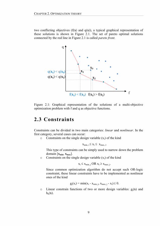
During an optimization process, several individuals (i.e. sets of values of the variables) are tested. For each of them, corresponding values of the objective functions are calculated. A process characterized by only one objective function is classified as single-objective optimization and identifies the solution with the individual with the lowest value of the objective function. Whenever several functions have to be minimized at the same time, the process takes the name of multi-objective optimization. In this case, if the objectives are conflicting, no unique solution which minimizes all of them simultaneously can be found. Instead, a set of solutions called pareto optimal solutions is identified. In order to understand what pareto solutions are, the concept of dominating solutions must be introduced. Considering as objective functions fi(x) with i = 1, 2, …, M, solution x1 dominates solution x2 if fi(x1) < fi(x2) for at least one index i and fi(x1) ≤ fi(x2) for all indices i. Considering this definition, pareto optimal solutions are not dominated by any other solution. In other words, starting from a pareto optimal solution, any change in the variables values that would improve one of the objective functions, would degrade one or more of the others. Considering
CHAPTER 2. OPTIMIZATION THEORY
9
two conflicting objectives (f(x) and q(x)), a typical graphical representation of these solutions is shown in Figure 2.1. The set of pareto optimal solutions connected by the red line in Figure 2.1 is called pareto front.
Figure 2.1: Graphical representation of the solutions of a multi-objective optimization problem with f and q as objective functions.
2.3 Constraints
Constraints can be divided in two main categories: linear and nonlinear. In the first category, several cases can occur:
o Constraints on the single design variable (xi) of the kind
xmin, i xi xmax, i.
This type of constraints can be simply used to narrow down the problem domain [xmin, xmax].
o Constraints on the single design variable (xi) of the kind
xi xmin, j OR xi xmax, j.
Since common optimization algorithm do not accept such OR-logic constraint, these linear constraints have to be implemented as nonlinear ones of the kind
gj(xi) = min(xi - xmin, j, xmax, j - xi) 0.
o Linear constrain functions of two or more design variables: gj(x) and hk(x).

2.4 OPTIMIZATION ALGORITHMS
10
The latter, together with nonlinear constraints, makes constrained optimization problems more difficult to handle than unconstrained ones. To address this issue, a strategy can be that of solving an equivalent unconstrained problem instead of the original constrained one using the penalty method (Griva, et al., 2009). The objective function f(x), which here is assumed to be unique for the sake of simplicity, is replaced by the penalized objective function in Eq. (2.1).
(x, , ) = f(x) + P(x, , ) (2.1)
P(x, , ) is the penalty term; it has several popular definitions and the one used in the present work is given in Eq. (2.2) (Yang, 2014).
P , , μ H g g H h h (2.2)
Thus, the penalty term is proportional to the magnitude of the constraints violations. In Eq. (2.2), j > 0 and k ≫ 1, while the terms Hj[gj(x)] and Hk[hk(x)] are defined in Eq. (2.3) and Eq. (2.4).
H g0ifg 0,1otherwise,
(2.3)
H h0ifh 0,1otherwise,
(2.4)
The penalty method, however, handles the constraints issue while computing the objective function; this implies all the intermediate steps between assigning the design variable values and computing the corresponding objective function. This entire process can be time consuming; an alternative could be to evaluate constraints as soon as the solution has been generated and discard it in case it is not feasible (direct approach).
2.4 Optimization algorithms
The only way to be sure to find the absolute minimum of the objective functions would be an exhaustive search, which consists in testing all possible values of the design variables. However, this technique is extremely time-consuming. In order to make the process more efficient based on the results of previous iterations, optimization algorithms have the role of creating new sets of variables to test in the current iteration. In other words, they are responsible of directing
CHAPTER 2. OPTIMIZATION THEORY
11
the search towards the domain areas that most highly contain the optimal solution based on previous experience. Optimization algorithms can be classified in several ways. However, it is worth remarking that classification of optimization algorithms is not binary: several algorithms combining two or more of the classes exist. One first distinction is between derivative-based and derivative-free algorithms. The first ones calculate the gradient of the objective function to guide the selection of the variables values for the next step. Derivative-free optimization algorithms, instead, use only the value of the objective function and do not compute any derivative. Therefore, derivative-based algorithms can be use only when the objective function is continuous and its derivatives can be computed, which is not always the case in structural optimization. Another possible classification is between deterministic and stochastic algorithms. Deterministic algorithms work in a mechanical deterministic manner without any random nature, while stochastic algorithms use randomization. As a consequence, the latter could escape the optimal solution at each iteration making the process more time-consuming or even unsuccessful. On the other hand, escaping a local minimum can be useful to increase the possibility of finding the global one. Lastly, optimization algorithms can be classified as local or global search algorithms. The first ones start from a set of variables values and update the solution moving to the improving configuration in its neighbourhood. Global search algorithms, instead, do not stick to the neighbourhood of the previous solution, but generate diverse solutions by exploring the search domain on a global scale by searching in regions not associated with the current best solution. This exploration is often done due to randomization. Two main limits of local search algorithms are evident: 1) whenever the solution approaches a local minimum it cannot escape, 2) the success of the search is strictly related to the initial configuration and, from a practical point of view, it relies on the experience and ability of the user who defines it. The other side of the coin is that local search algorithms are much faster and efficient whenever those two problems do not occur. Finally, metaheuristic optimization algorithms can be defined as hybrid algorithms with a trade-off between global exploration and local search. In many of them, the global exploration is possible due to randomization, which classifies them as stochastic. In general, no algorithm is better than another for all problems; therefore, it is important to consider the type of objective function and its dependence on the variables of the specific problem to select the most suitable algorithm.


13
3 Optimization of RC beam bridges
This chapter presents the software application for optimal design of road beam bridges that has been developed in MATLAB®. The computer code aims to find, in a reasonable time, the solution that minimizes the investment cost or the environmental impact of the entire structure. One of the most important features of this work is the focus on the complete bridge instead of optimizing individual members; indeed, both the static system configuration and the deck cross section sizes are considered as design variables.
3.1 Design and optimization procedure
In the following, an iterative optimization procedure divided in several modules (Figure 3.1) is presented. In Module 1, a set of values for the design variables that describe the three-dimensional model of the bridge is assumed. At this point, an external FEM software able to handle moving traffic loads and all the required load combinations is called by the main program. In the present work, a Swedish FEM software called Strip-Step 3 has been used and Timoshenko beam elements have been employed. In Module 2, it applies the loads and their combinations requested by the Eurocode 1 (European Commitee for Standardization, 2003) and in Module 3 it calculates the internal forces and moments in the bridge deck. These values are then used in Module 4 to calculate the deck reinforcement required by the Eurocode 2 (European Commitee for
Chapter

3.1 DESIGN AND OPTIMIZATION PROCEDURE
14
Standardization, 2005) to satisfy the Ultimate Limit State (ULS) and the Serviceability Limit State (SLS). At this point the geometry of the bridge is completely defined and material quantities can be computed in Module 5. Finally, in Module 6, the investment cost and the environmental impact of the bridge are calculated. Once the last module has been reached, an optimization algorithm varies the values of the design variables of Module 1 and the cycle starts again. The process stops when one of the stopping criteria of the optimization algorithm is met.
Figure 3.1: Design and optimization process.
In this work, the design variables are:
Number of spans (in an admissible range defined by the user), Longitudinal position of each intermediate pier, Type of connection between each intermediate pier and the deck, Dimensions of the concrete deck cross sections at several locations in
each span (the number of cross sections per span is defined by the user). Therefore, the total number of variables is function of the number of spans. Since optimization algorithms require a fixed number of design variables, it was not possible to optimize all variables at the same time. Therefore, the approach proposed by El Mourabit (2016) has been adopted: the problem has been divided in two consecutive levels and several sub-levels. Level 1 has the goal of optimizing the static system by defining the first three groups of variables listed above, while Level 2 has the goal of optimizing the cross sections dimensions. Level 1, in turn, is divided in sub-levels: each of them can be considered as an optimization problem to be solved through the procedure of Figure 3.1. The deck
CHAPTER 3. OPTIMIZATION OF RC BEAM BRIDGES
15
cross-section is assumed constant, with dimensions defined by the user. In each sub-problem the number of spans is fixed, thus the only variables are the intermediate piers locations and their connections with the superstructure. At the end of level 1, the optimal static system configurations for all sub-problems (i.e. for all possible numbers of spans) are compared. The one resulting in the lowest investment cost or environmental impact is selected and used in level 2. The latter follows the procedure of Figure 3.1 as well, but has all cross-sectional dimensions of the deck as design variables. Dividing the procedure in two levels not only solves the problem of varying number of variables but also allows for finding the optimal solution in a faster way by reducing the total number of variables treated simultaneously.
3.2 Objective functions
The developed software performs a single-objective optimization using investment cost or environmental impact as fitness function. However, during the process, both values are calculated; therefore, once the investment cost has been minimized, the associated environmental impact is computed and vice versa.
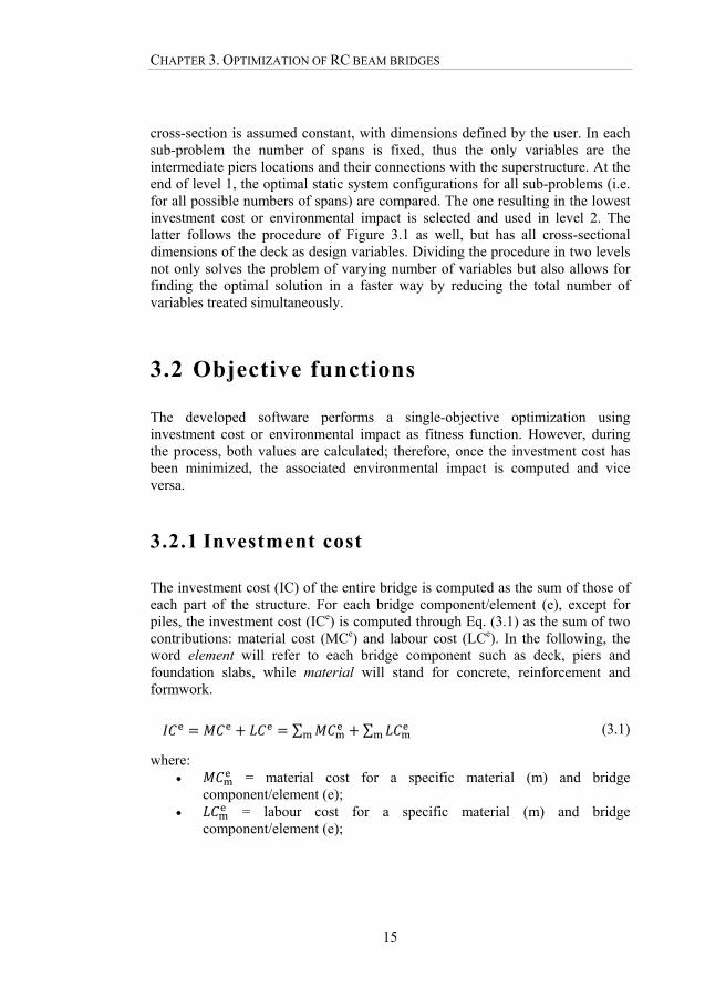
3.2.1 Investment cost
The investment cost (IC) of the entire bridge is computed as the sum of those of each part of the structure. For each bridge component/element (e), except for piles, the investment cost (ICe) is computed through Eq. (3.1) as the sum of two contributions: material cost (MCe) and labour cost (LCe). In the following, the word element will refer to each bridge component such as deck, piers and foundation slabs, while material will stand for concrete, reinforcement and formwork.
∑ ∑ (3.1)
where: = material cost for a specific material (m) and bridge
component/element (e); = labour cost for a specific material (m) and bridge
component/element (e);

3.2 OBJECTIVE FUNCTIONS
16
For what concern piles, since their construction and installation is different from that of other components, investment cost (ICpile) is computed as in Eq. (3.2).
(3.2)
where: = unit price for pile including material and labour (Table 3.1); = length of the pile.
Table 3.1: Unit prices for piles.
Pyle type Unit price Cpile (SEK/m)
Concrete piles SP1 450
Concrete piles SP2 550
Concrete piles SP3 700
Steel core piles ϕ90 3500
Steel core piles ϕ100 4250
Steel core piles ϕ120 4750
Steel core piles ϕ150 5500
3.2.1.1 Material cost
Material cost is purely dependent on the national and international market and its fluctuation and on the amount of material (i.e. solution dimensions). Considering a specific material (m) and element (e), it is calculated as in Eq. (3.3).
(3.3)
where: = unit price for material m; = amount of material m in the considered element e.

CHAPTER 3. OPTIMIZATION OF RC BEAM BRIDGES
17
Values used in this work can be found in Table 3.2. The formwork has more than one value depending on the element it refers to: indeed, the type of material used is different based on the shape and the structural role of the element to be constructed.
Table 3.2: Unit prices for materials (piers types in Figure 3.2).
Material Unit price Cm
Concrete C32/40 17001 SEK/m3
Concrete C35/45 1800 SEK/m3
Concrete C50/60 2000 SEK/m3
Reinforcement 9000 SEK/ton
Formwork: deck
Distance from the ground ≤ 5 m 10002 SEK/m2
Formwork: deck
Distance from the ground: 5 - 7 m 1250 SEK/m2
Formwork for piers, type 1 300 SEK/m2
Formwork for piers, type 2 700 SEK/m2
Formwork for foundation slabs 200 SEK/m2
3.2.1.2 Labour cost and constructability coefficients
To properly evaluate the labour cost, practical considerations about constructability are necessary. Indeed, what determines the labour cost is the time needed to build an element, which is not only related to the amount of material, but also to the complexity of the considered element. Based on the
1 Concrete prices include transport for 20-30 km. Consider an increase of 50 SEK/m3 for every 10 km of additional distance site - concrete supplier. 2 The price of the formwork for the deck includes also scaffolding.

3.2 OBJECTIVE FUNCTIONS
18
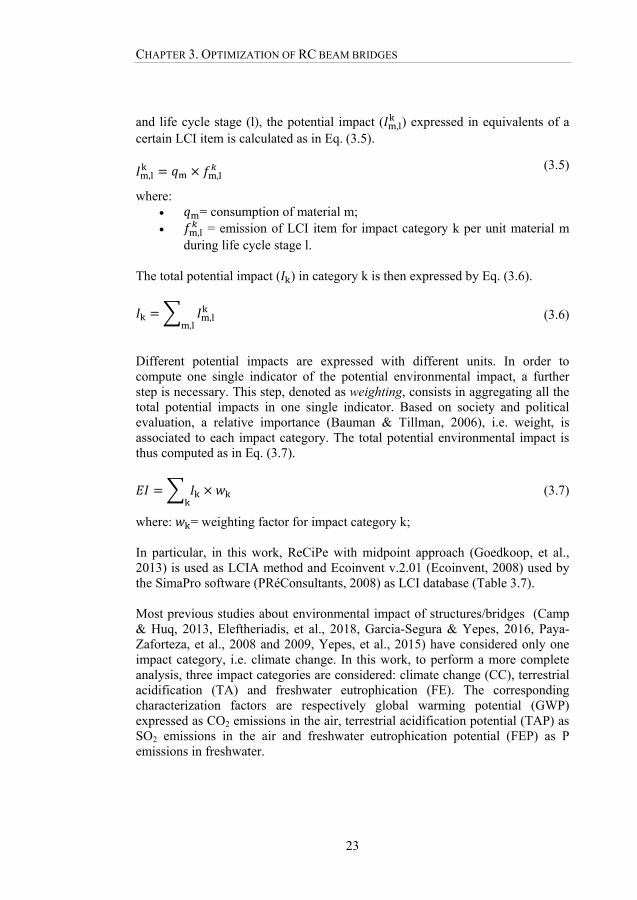
shape, location and function of the element, the time needed to build it can vary significantly. The following examples will clarify the concept. Example 1: When constructing a pier, if concrete was poured all at once, the pressure on the formwork at the base of the column would be too high with the risk of formwork collapse. Hence, it is necessary to divide the process in steps: i) pour concrete up to a reference height, ii) vibrate, iii) wait for the material to start hardening and then repeat steps i-iii. This procedure is not necessary when constructing e.g. a slab foundation since the thickness is not big enough to give rise to excessive pressure on the formwork. As a consequence, the labour time in the case of a unit volume of concrete for slab foundations is less than for piers. Example 2: One element can have several shapes as for the deck or the piers in Figure 3.2; as a consequence, the labour cost for the same amount of material can assume several values. Indeed, e.g. reinforcement labour is of increasing difficulty and thus takes longer going from cross-section type 1 to type 3.
Figure 3.2: (a) Possible cross-section shapes for the bridge deck and (b) Possible pier types.
(a) (b)
CHAPTER 3. OPTIMIZATION OF RC BEAM BRIDGES
19
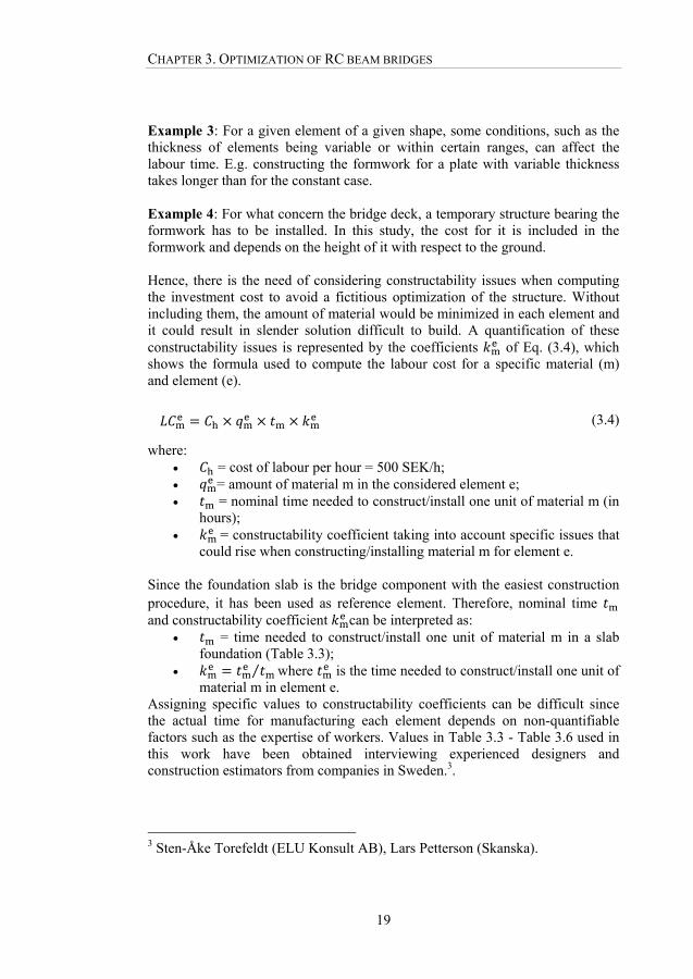
Example 3: For a given element of a given shape, some conditions, such as the thickness of elements being variable or within certain ranges, can affect the labour time. E.g. constructing the formwork for a plate with variable thickness takes longer than for the constant case. Example 4: For what concern the bridge deck, a temporary structure bearing the formwork has to be installed. In this study, the cost for it is included in the formwork and depends on the height of it with respect to the ground. Hence, there is the need of considering constructability issues when computing the investment cost to avoid a fictitious optimization of the structure. Without including them, the amount of material would be minimized in each element and it could result in slender solution difficult to build. A quantification of these constructability issues is represented by the coefficients of Eq. (3.4), which shows the formula used to compute the labour cost for a specific material (m) and element (e).
(3.4)
where: = cost of labour per hour = 500 SEK/h; = amount of material m in the considered element e; = nominal time needed to construct/install one unit of material m (in
hours); = constructability coefficient taking into account specific issues that
could rise when constructing/installing material m for element e. Since the foundation slab is the bridge component with the easiest construction procedure, it has been used as reference element. Therefore, nominal time and constructability coefficient can be interpreted as:
= time needed to construct/install one unit of material m in a slab foundation (Table 3.3);
⁄ where is the time needed to construct/install one unit of material m in element e.
Assigning specific values to constructability coefficients can be difficult since the actual time for manufacturing each element depends on non-quantifiable factors such as the expertise of workers. Values in Table 3.3 - Table 3.6 used in this work have been obtained interviewing experienced designers and construction estimators from companies in Sweden.3.
3 Sten-Åke Torefeldt (ELU Konsult AB), Lars Petterson (Skanska).

3.2 OBJECTIVE FUNCTIONS
20
Lastly, two possible types of pier-deck connection have been considered in the study: fixed and movable bearing. Fixed bearings are those where all rotations and translations are fixed. Movable bearing, instead, allow for longitudinal translation and bending rotation. Fixed bearings cause an increase of the internal forces and moments in the substructure. However, the developed program does not design the piers and the reinforcement in the foundation slab, but assumes pre-assigned values. Thus, a multiplying factor equal to 1.2 has been employed to increase the cost of the substructure (pier, foundation slab and piles if present) in case of fixed connection.
Table 3.3: Nominal time for material installation.
Material Time Unit
Concrete 1 h/m3
Reinforcement 20 h/ton
Formwork 1 h/m2
Table 3.4: Constructability coefficients for concrete. Cross-section and piers types are shown respectively in Figure 3.2.
Element Constructability
coefficient Description
Deck 1 Cross-section type 1
Deck 1.1 Cross-section type 2
Deck 1.3 Cross-section type 3
Piers 1 Pier type 1
Piers 2 Pier type 2
Foundation slabs 1 -

CHAPTER 3. OPTIMIZATION OF RC BEAM BRIDGES
21
Table 3.5: Constructability coefficients for reinforcement. Cross-section and piers types are shown respectively in Figure 3.2.
Element Constructability
coefficient Description
Deck 1 Cross-section type 1
Deck 1.15 Cross-section type 2
Deck 1.25 Cross-section type 3
Piers 1.2 Pier type 1
Piers 1.7 Pier type 2
Foundation slabs 1 -
Table 3.6: Constructability coefficients for formwork. Piers types are shown Figure 3.2b.
Element Constructability
coefficient Description
Deck 2 Distance from the ground:
up to 5 m
Deck 2.3 Distance from the ground:
5 - 7 m
Piers 1.2 Pier type 1
Piers 2.5 Pier type 2
Foundation slabs 1 -
3.2 OBJECTIVE FUNCTIONS
22
3.2.2 Environmental impact
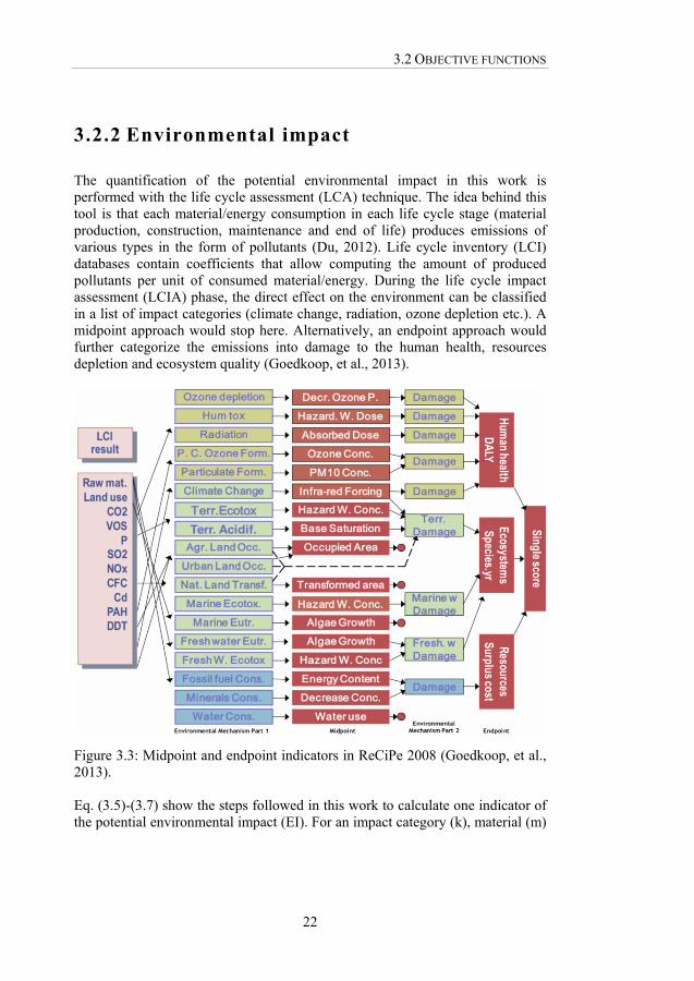
The quantification of the potential environmental impact in this work is performed with the life cycle assessment (LCA) technique. The idea behind this tool is that each material/energy consumption in each life cycle stage (material production, construction, maintenance and end of life) produces emissions of various types in the form of pollutants (Du, 2012). Life cycle inventory (LCI) databases contain coefficients that allow computing the amount of produced pollutants per unit of consumed material/energy. During the life cycle impact assessment (LCIA) phase, the direct effect on the environment can be classified in a list of impact categories (climate change, radiation, ozone depletion etc.). A midpoint approach would stop here. Alternatively, an endpoint approach would further categorize the emissions into damage to the human health, resources depletion and ecosystem quality (Goedkoop, et al., 2013).
Eq. (3.5)-(3.7) show the steps followed in this work to calculate one indicator of the potential environmental impact (EI). For an impact category (k), material (m)
Figure 3.3: Midpoint and endpoint indicators in ReCiPe 2008 (Goedkoop, et al.,2013).
CHAPTER 3. OPTIMIZATION OF RC BEAM BRIDGES
23
and life cycle stage (l), the potential impact ( , ) expressed in equivalents of a certain LCI item is calculated as in Eq. (3.5).
, , (3.5)
where: = consumption of material m; , = emission of LCI item for impact category k per unit material m
during life cycle stage l.
The total potential impact ( ) in category k is then expressed by Eq. (3.6).
,,
(3.6)
Different potential impacts are expressed with different units. In order to compute one single indicator of the potential environmental impact, a further step is necessary. This step, denoted as weighting, consists in aggregating all the total potential impacts in one single indicator. Based on society and political evaluation, a relative importance (Bauman & Tillman, 2006), i.e. weight, is associated to each impact category. The total potential environmental impact is thus computed as in Eq. (3.7).
(3.7)
where: = weighting factor for impact category k; In particular, in this work, ReCiPe with midpoint approach (Goedkoop, et al., 2013) is used as LCIA method and Ecoinvent v.2.01 (Ecoinvent, 2008) used by the SimaPro software (PRéConsultants, 2008) as LCI database (Table 3.7). Most previous studies about environmental impact of structures/bridges (Camp & Huq, 2013, Eleftheriadis, et al., 2018, Garcia-Segura & Yepes, 2016, Paya-Zaforteza, et al., 2008 and 2009, Yepes, et al., 2015) have considered only one impact category, i.e. climate change. In this work, to perform a more complete analysis, three impact categories are considered: climate change (CC), terrestrial acidification (TA) and freshwater eutrophication (FE). The corresponding characterization factors are respectively global warming potential (GWP) expressed as CO2 emissions in the air, terrestrial acidification potential (TAP) as SO2 emissions in the air and freshwater eutrophication potential (FEP) as P emissions in freshwater.
3.2 OBJECTIVE FUNCTIONS
24
Concerning the lifecycle stages, a cradle-to-gate approach, which considers only the material production phase, has been chosen for several reasons. First of all, previous studies (Flower & Sanjayan, 2007, Du & Karoumi, 2013) have shown that this stage for bridges is the most influential one. Furthermore, the main aim of this work is to find the best solution, in terms of static system and dimensions, for one particular structural type (i.e. reinforced concrete beam bridge). The construction method is assumed to be the same regardless of the solution. As a consequence, it is reasonable to expect that this phase will not significantly affect the choice of one solution instead of another. Moreover, due to their re-use, the production of material for temporary structures (i.e. scaffolding and formwork) hasn’t been included in the calculations. Thus, only concrete, steel for reinforcement bars and RC for piles have been used as materials in Eq. (3.5) and Eq. (3.6). Finally, concerning the weighting system, results of previous studies with similar aim (Yavari, et al., 2017 and Ahlroth & Finnveden, 2011) show no great differences between the solutions of the optimization problem obtained using two different weighting systems that monetarize the environmental impact: Ecotax02 (Finnveden, et al., 2006) and Ecovalue (Ahlroth & Finnveden, 2011, Finnveden, et al., 2013). The values in Table 3.7 help understanding why no significant differences have been obtained with the two weighting systems. Both concrete and reinforcement steel in production phase emit much more CO2 than SO2 or P per unit material. As a consequence, regardless of the adopted weighting system, climate change is always the leading impact category. Therefore, Ecovalue12 is used in this work since it is the most recent one. It aggregates all the emissions in a monetary value based on individual willingness-to-pay for the loss of benefits due to environmental degradation (Ahlroth & Finnveden, 2011) and its significant values for this work are shown in Table 3.8.

CHAPTER 3. OPTIMIZATION OF RC BEAM BRIDGES
25
Table 3.7: Emission of LCI items from Ecoinvent database (Ecoinvent, 2008).
Material m Impact category
k Unit
Concrete C25/30
CC 261 kg CO2/m3
TA 0.44 kg SO2/m3
FE 0.014 kg P/m3
Other concrete
(form C30/37 to C55/67)
CC 288 kg CO2/m3
TA 0.50 kg SO2/m3
FE 0.016 kg P/m3
Reinforcement A500HW
CC 1446 kg CO2/ton
TA 4.74 kg SO2/ton
FE 0.87 kg P/ton
RC piles C40/50
CC 404 kg CO2/m
TA 0.88 kg SO2/m
FE 0.085 kg P/m
Table 3.8: Ecovalue12 weighting set (Finnveden, et al., 2013).
Impact category Weighting factor
Global warming 2.85 SEK/kg CO2-eq
Terrestrial acidification 30 SEK/kg SO2-eq
Freshwater eutrophication 670 SEK/kg P

3.3 CONSTRAINTS
26
3.3 Constraints
When it comes to structural optimization, two main types of constraints have to be considered: structural and operational constraints. To the first category belong all the requirements of the Eurocodes and the national codes regarding ULS and SLS. Furthermore, one must remember that bridges are infrastructures built in order to cross obstacles such as rivers, highways, footpaths etc. Therefore, there are areas where piers can’t be place and minimum vertical clearance must be guaranteed. Such limitations together with others based on the common practice fall in the previously mentioned category of operational constraints.
3.3.1 ULS and SLS
3.3.1.1 Beam bridge deck
In this work, the deck cross-sections are checked for crack width (w), bending moment (M), shear (V) and torsion (T). In the Eurocode 2, they all have the form
E ≤ R or w ≤ wmax where R is the resistance and E the effect of the action. Following the general mathematic formulation of a nonlinear optimization problem shown in chapter 2, they have been expresses as
g 1 0 or g 1 0.
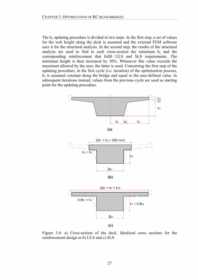
At the current stage, the focus has been on cross-sections with the shape shown in Figure 3.4a, which has been simplified as in Figure 3.4b and c for the ULS and SLS checks in the longitudinal direction. To better understand the formulation of the constraints in this section, the reinforcement design procedure is explained in the following. Before starting the optimization, the user has to assign all dimensions of the deck cross-section and decide to keep constant the web width (2b1) or the web inclination (b2/h1). All dimensions of the deck except for the web height (h1) are kept constant along the bridge during level 1. The web height instead is constantly updated and varies along the deck.
CHAPTER 3. OPTIMIZATION OF RC BEAM BRIDGES
27
The h1 updating procedure is divided in two steps. In the first step, a set of values for the web height along the deck is assumed and the external FEM software uses it for the structural analysis. In the second step, the results of the structural analysis are used to find in each cross-section the minimum h1 and the corresponding reinforcement that fulfil ULS and SLS requirements. The minimum height is then increased by 30%. Whenever this value exceeds the maximum allowed by the user, the latter is used. Concerning the first step of the updating procedure, in the first cycle (i.e. iteration) of the optimization process, h1 is assumed constant along the bridge and equal to the user-defined value. In subsequent iterations instead, values from the previous cycle are used as starting point for the updating procedure.
(b)
(c)
Figure 3.4: a) Cross-section of the deck. Idealized cross sections for thereinforcement design in b) ULS and c) SLS
(a)
3.3 CONSTRAINTS
28
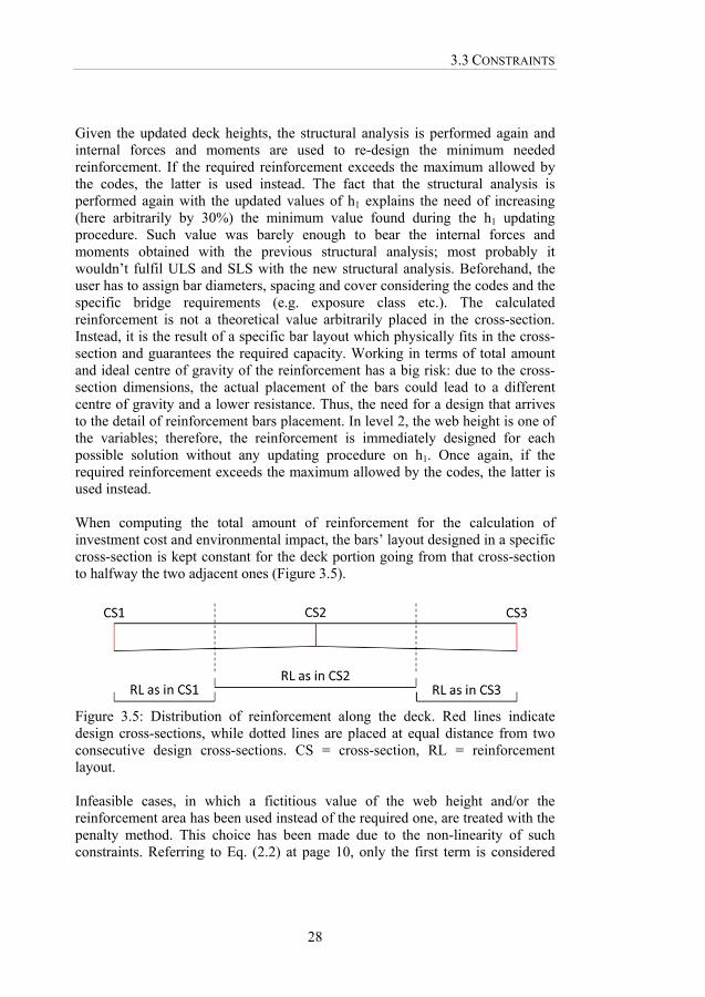
Given the updated deck heights, the structural analysis is performed again and internal forces and moments are used to re-design the minimum needed reinforcement. If the required reinforcement exceeds the maximum allowed by the codes, the latter is used instead. The fact that the structural analysis is performed again with the updated values of h1 explains the need of increasing (here arbitrarily by 30%) the minimum value found during the h1 updating procedure. Such value was barely enough to bear the internal forces and moments obtained with the previous structural analysis; most probably it wouldn’t fulfil ULS and SLS with the new structural analysis. Beforehand, the user has to assign bar diameters, spacing and cover considering the codes and the specific bridge requirements (e.g. exposure class etc.). The calculated reinforcement is not a theoretical value arbitrarily placed in the cross-section. Instead, it is the result of a specific bar layout which physically fits in the cross-section and guarantees the required capacity. Working in terms of total amount and ideal centre of gravity of the reinforcement has a big risk: due to the cross-section dimensions, the actual placement of the bars could lead to a different centre of gravity and a lower resistance. Thus, the need for a design that arrives to the detail of reinforcement bars placement. In level 2, the web height is one of the variables; therefore, the reinforcement is immediately designed for each possible solution without any updating procedure on h1. Once again, if the required reinforcement exceeds the maximum allowed by the codes, the latter is used instead. When computing the total amount of reinforcement for the calculation of investment cost and environmental impact, the bars’ layout designed in a specific cross-section is kept constant for the deck portion going from that cross-section to halfway the two adjacent ones (Figure 3.5).
Figure 3.5: Distribution of reinforcement along the deck. Red lines indicate design cross-sections, while dotted lines are placed at equal distance from two consecutive design cross-sections. CS = cross-section, RL = reinforcement layout. Infeasible cases, in which a fictitious value of the web height and/or the reinforcement area has been used instead of the required one, are treated with the penalty method. This choice has been made due to the non-linearity of such constraints. Referring to Eq. (2.2) at page 10, only the first term is considered
CHAPTER 3. OPTIMIZATION OF RC BEAM BRIDGES
29
and the magnitude of the constraints violations for each cross-section is computed as in Eq. (3.8)-(3.10).
g/
/
/
1 (3.8)
g _ 1 (3.9)
[(6.29)-EC2]
g 1 (3.10)
where: UE/LE = upper edge/lower edge; Ed = action on the cross-section; Rd = resistance of the cross-section.
3.3.1.2 Cantilever slab
In addition to the above mentioned constraints in the longitudinal direction, cross-sections are verified and reinforcement is designed in the cantilever slab for bending, shear and limited crack width. All possible locations of vehicles on the cantilever are considered together with the scenario of missing edge beam due to replacement. Load models LM1 and LM2 are considered as required by Eurocode 1. In this stage, the cantilever has been isolated from the rest of the deck. It has been studied as a slab with varying thickness, free in correspondence of the edge beam and clamped at the opposite edge. The effect of the edge beam is taken into account by extending the slab. The length of the added portion is computed in such a way that it has the same flexural rigidity of the edge beam (Veganzones Muñoz, 2016). For every considered load scenario, the flexural moment is computed at the clamped edge using the influence surfaces proposed by Homberg & Ropers, (1965). Shear forces, instead, are computed in the most critical cross-sections according to Swedish regulations (Trafikverket, 2011). In the current practice, shear reinforcement in the cantilever slab is avoided. Therefore, bending reinforcement is calculated both for the moment at the clamped edge and to provide enough shear resistance in absence of stirrups. The required reinforcement varies along the cantilever; however, to reduce complexity during construction, the final design can contain a maximum of two

3.3 CONSTRAINTS
30
groups of reinforcement bars. One group goes from edge beam to edge beam all along the deck flange and a shorter group connects the midpoints of the two cantilever slabs. To account for infeasible solutions, once the reinforcement has been designed, the possible constraint violation is computed using Eq. (3.8) and Eq. (3.9) without torsion.
3.3.2 Infeasible regions for piers
As previously mentioned, bridges are built to cross obstacles. The consequence is that there are specific regions where it is not possible to place piers. In level 1, such constraints have the form
xi xmin, j OR xi xmax, j,
that, as explained in section 2.3, are implemented in the non-linear form
gj(xi) = min(xi - xmin, j, xmax, j - xi) 0,
where xmin, j and xmax, j represent the coordinate of the obstacle to cross. Since it has been decided to avoid non-linearly constrained problems, the direct approach has been employed in this case. For solution with piers in infeasible regions no structural analyses are performed. Instead, a fictitious value for the objective function is assumed. To make the optimization algorithm discard such solutions in favour of feasible ones, this default value is set at one order of magnitude higher than the expected output for a feasible solution.
3.3.3 Minimum vertical clearance
Concerning the minimum vertical clearance, it is checked in both levels since the cross-section heights vary in both. The magnitude of the constraint violation is computed as in Eq. (3.11).
g . .,
1 (3.11)
where:

CHAPTER 3. OPTIMIZATION OF RC BEAM BRIDGES
31
= height under the bridge deck in a cross-section; , = the minimum vertical clearance for j-th obstacle.
Once the number of design cross-section per span is defined by the user, they are placed along the span at equal distance one from each other. Therefore, there is no guarantee that they are aligned with regions with minimum vertical clearance. As a consequence, is calculated by linearly interpolating height values in design sections. The constraint on the minimum vertical clearance in level 2 is thus a linear function of more than one variable. In level 1 instead, the cross-section heights are not directly variables of the problem and they are computed as explained in section 3.3.1; thus, in this case the constraint is non-linear. As explained in section 2.3, linear constraints of more than one variables and non-linear once are difficult to handle, thus the use of the penalty method again.
3.3.4 Cross-section dimensions and span length
The only linear constraints considered in this work are defined by the user in terms of limitations on each cross-section dimension and on span lengths. Since in level 2 cross-section dimensions are the variables of the problem, these linear constraints are simply used to narrow down the searching space [xmin, xmax]. Such procedure can’t be applied to the limitation of span lengths since each length is function of two variables of level 1 (i.e. pier locations). Therefore, a linear constraint is given as input to the optimization algorithm selected for level 1 and is implemented in the form of Eq (3.12).
∙ (3.12)
where: = matrix of 1 and 0 built such that each row of the product ∙
represents the length of one of the spans; = vector containing the minimum and maximum values for each span
length; = vector containing the variables of level 1.
3.4 OPTIMIZATION ALGORITHMS
32
3.4 Optimization algorithms
The selection of the type of optimization algorithm to use is influenced by the nature of the problem and of the objective functions. Moreover, when it comes to practical problem, computational time plays an important role as well. Regardless of the algorithm used, in order to make the optimization procedure faster, a memory system has been integrated. First of all, the user has to choose accuracies for the variables (decimetres for pier locations and centimetres for cross-section dimensions are suggested). At the beginning of iterations, variable values are rounded according to the accuracies. Then, results for every studied individual are saved in a continuously updated database and re-used in future iterations. In such a way, the optimization algorithm still works with continuous instead of difficult-to-handle discrete variables but a large portion of the computational time is saved. Indeed, the FEM software is not called for individuals that differ from those in the database by less than the preassigned accuracies. Indeed, the most time-consuming step of the procedure explained in section 3.1 is the use of a FEM software application. Such a step is performed for each individual (i.e. set of tested variables) of each iteration. Furthermore, in level 1, the structural analysis is performed twice per individual as explained in section 3.3.1. Considering this and the large number of variables in level 2, it is not reasonable to employ exhaustive search in this problem. Instead, using an optimization algorithm that searches in several areas of the domain to find the best solution in the shortest time is preferable. Thus, the combination of local and global search is fundamental for this problem and metaheuristic optimization algorithms could be an appropriate choice. Especially in level 1, another issue points towards the choice of metaheuristic optimization algorithms: some variables are continuous (i.e. pier locations), while others are discontinuous (i.e. pier-deck connection can only be fixed or movable). The complexity of a mixed-integer optimization problem and the consequent discontinuity of the objective function can be handled by the robustness of metaheuristic algorithms. Both in level 1 and 2, the two objective functions are strictly related to the amount of materials. Concerning concrete, this amount is the result of geometric calculation based only on the variable values. The reinforcement amount instead is the result of a design procedure which takes into account several load scenarios and verifications. Thus, the relationship between the variables and the objective function is implicit and non-continuous. As a consequence, derivative-
CHAPTER 3. OPTIMIZATION OF RC BEAM BRIDGES
33
based optimization algorithms can’t be used for the studied problem in neither of the two levels. Moreover, in level 1 the deck heights are computed based on the results of a structural analysis carried out with provisional cross-sections heights from the previous iteration (section 2.3.3). Such provisional heights have no relation with the variable values of the current iteration. It results in the introduction of random noise in the objective function of level 1, which suggests the use of stochastic optimization algorithms. Furthermore, the fact that stochastic algorithms can be slower than deterministic ones is not a major problem in level 1 since the number of variables is much lower than in level 2. For all the reasons listed above, two gradient-free optimization algorithms have been chosen: Genetic Algorithm (GA) for level 1 and Pattern Search (PS) for level 2. GA can be classified as a metaheuristic optimization algorithm that combines local and global search using randomization (i.e. stochastic). On the other hand, PS is a deterministic local search algorithm. Level 2 shows fewer difficulties than level 1 and a more straight-forward relationship variables-objective function; therefore, a local search algorithm such as PS is expected to work well. The author tried to apply GA also to level 2; however, it performed worse compared to PS. In the present work, the GA and PS (also called direct search) provided in MATLAB® Optimization Toolbox (The MathWorks, Inc., R2016b) has been used. The general way of working of GA and PS is explained in the following together with specific options selected for the current work. When not specified, the default option has been used. For more detailed information and for possible alternatives, the author suggests reading the toolbox guide (The MathWorks, Inc., R2018b).
3.4.1 Genetic Algorithm
Genetic algorithm (GA) is a metaheuristic optimization technique inspired by Darwin’s Theory of Evolution (McCall, 2005) and used to solve several structural optimization problems (Camp, et al., 2002, Govindaraj & Ramasamy, 2005, Srinivas & Ramanjaneyulu, 2007).

3.4 OPTIMIZATION ALGORITHMS
34
3.4.1.1 Population
The algorithm starts from a population made of a user-defined number of individuals. Each of them is characterized by a specific set of genes (i.e. values of the design variables) randomly selected. In order to generate a new population, the algorithm performs the following preliminary steps (The MathWorks, Inc., R2018b):
The objective function is evaluated for all individuals of the current population, thus a set of raw fitness scores is generated.
To get a measure of how fit individuals are for survival, a scaling function is applied to raw fitness scores to get expectation values.
Based on expectation values, the parents for the next generation are selected in a stochastic way. However, individuals with lower raw fitness score (i.e. more fit for survival) have higher probability of being selected.
The new generation is then formed by: Elite children: individuals identical to those with the lowest raw fitness
scores of the previous population. Mutation children: individuals obtained by randomly modifying the
genes of one parent. Crossover children: individuals created extracting genes from two
parents. The numbers of children belonging to the three categories listed above are defined by the user. Referring to the concepts introduced in section 2.4, elite and crossover children represent the local component of the search, while mutation ones the global component obtained through randomization.
3.4.1.2 Default stopping criteria
The algorithm stops generating new populations when one of its stopping criteria is met. Some stopping criteria are introduced in order to limit the computational time:
The algorithm stops when the maximum number of iterations (i.e. new populations) has been reached.
The algorithm stops when the time limit has been exceeded. The risk of stopping the process due to one of them is that the algorithm doesn’t manage to get close enough to the optimum. To avoid it, default values for such stopping criteria are defined in a way that the algorithm generates a really high
CHAPTER 3. OPTIMIZATION OF RC BEAM BRIDGES
35
number of populations. Thus, using the default values imply long computational time. In this work, instead of modifying the default values to make the process faster, other strategies have been used: a memory system has been integrated and customized stopping criteria have been added. Another stopping criterion is particularly useful when the aim is to limit the fitness function value instead of minimizing it:
The algorithm stops when the lowest raw fitness score is lower than a preassigned minimum.
However, such a criterion doesn’t guarantee the minimum but only an upper limit of the objective function. Thus, the default value that has been used in this work is very low. Finally, the last two stopping criteria are based on convergence towards the optimal solution:
The algorithm stops when there has been no improvement in the objective function for a certain amount of time.
For each population, the algorithm saves the minimum raw fitness score. It computes the relative average change in these values over a user-defined number of consecutive iterations. The algorithm stops when such average is lower than a threshold.
Concerning the first one, the time limit has to be set quite high. Indeed, it is not uncommon that several consecutive iterations have the same optimum even far from convergence. Regarding the second one, the average threshold would represent the saving of the objective function that can be considered non-significant for the studied problem. However, the default stopping criterion computes the average over all consecutive iterations regardless of the fact that they are improving or not (i.e. zero relative change). In such a way, the non-improving iterations lower the average and make the threshold loose its original meaning. The solution to this issue would be increasing the number of iterations to reduce the influence of non-improving ones while decreasing the threshold. However, this would lead to a more time-consuming process. Moreover, how much the threshold should be reduced is unclear. The solution proposed in this work is a customized stopping criterion that follows the same idea but gets rid of the above mentioned problems.
3.4.1.3 Customized stopping criteria
Two customized stopping criteria have been added to the default ones of GA. The first one is a more user-friendly version of the last stopping
criterion of section 3.4.1.2. The customized stopping criterion, considers only the improving iterations. Thus, the process is faster and
3.4 OPTIMIZATION ALGORITHMS
36
the definition of the threshold and the number of iterations to compute the average on is more straight-forward for the user.
When the optimal solution is approached, the amount of non-improving iterations increases. The risk is that the process could keep going because the algorithm doesn’t find enough improving iterations to compute the average on. In these situations, it has been noticed that GA tends to create population of almost identical individuals. Therefore, the second ad hoc stopping criterion consists in terminating the optimization when a user-defined amount of individuals of the current population are identical and no improvement in the fitness function has been achieved from the previous iteration.
To prove the efficiency of the customized optimization algorithms with integrated memory system, a simple example with only two spans (i.e. 2 variables in level 1) has been considered. Results showed a reduction of 66% in the computational time with no significant differences in the optimal solution.
3.4.2 Pattern Search
Pattern Search (PS), also known as direct search, is an optimization technique based on examination of trial solutions, comparison with the current best solution and consequent individuation of the next set of trail solutions (Hooke & Jeeves, 1961). This algorithm has previously been applied to solve structural optimization problems (Surtees & Tordoff, 1981, Yavari, et al., 2016 and 2017).
3.4.2.1 Trial solutions and polls
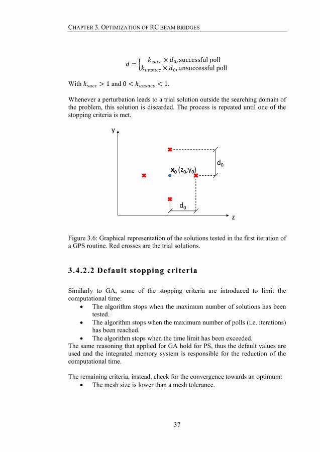
The generalized pattern search (GPS) method used in this work (The MathWorks, Inc., R2018b) starts from an initial solution (x0) and an initial mesh size (d0). During the first iteration, the value of the objective function in x0 is computed and a first set of trial solutions is tested. They are defined starting from the variable values of the initial solution and perturbing one of them at the time of ± d0. In a bi-dimensional problem (z and y as variables), the trial solutions would be those of Figure 3.6. The value of the objective function for the trial solutions is compared with that of the initial point. If the best solution results being the starting point, the poll occurred to be unsuccessful, otherwise, it is defined as successful poll. The starting point (i.e. the equivalent to the centre in Figure 3.6) for the next iteration is the best solution of the current one. The mesh size varies as follows:
CHAPTER 3. OPTIMIZATION OF RC BEAM BRIDGES
37
, successfulpoll, unsuccessfulpoll
With 1 and 0 1.
Whenever a perturbation leads to a trial solution outside the searching domain of the problem, this solution is discarded. The process is repeated until one of the stopping criteria is met.
Figure 3.6: Graphical representation of the solutions tested in the first iteration of a GPS routine. Red crosses are the trial solutions.
3.4.2.2 Default stopping criteria
Similarly to GA, some of the stopping criteria are introduced to limit the computational time:
The algorithm stops when the maximum number of solutions has been tested.
The algorithm stops when the maximum number of polls (i.e. iterations) has been reached.
The algorithm stops when the time limit has been exceeded. The same reasoning that applied for GA hold for PS, thus the default values are used and the integrated memory system is responsible for the reduction of the computational time. The remaining criteria, instead, check for the convergence towards an optimum:
The mesh size is lower than a mesh tolerance.
3.4 OPTIMIZATION ALGORITHMS
38
After a successful poll, the improvement in the objective function is lower than a function tolerance and the mesh size is lower than a pre-assigned value.
After a successful poll, both the mesh size and the distance between the last two best solutions are lower than a pre-assigned value.
Concerning the first one, with a small enough tolerance and d0 far from this value, it represents convergence to a minimum because the mesh size decreases only during unsuccessful polls. Therefore, very low values can be reached only after a long series of unsuccessful polls (i.e. polls pointing at the same solution, the optimal one). The other stopping criteria, instead, terminate the process when the changes in the solutions and the corresponding objective functions become insignificant. One problem of this algorithm is hidden behind the concept of mesh size. Indeed, as explained in section 3.4.2.1, the trial solutions are obtained perturbing one variable at the time with the same mesh regardless of the nature of the variables and of its domain. Thus, the same mesh size can be very little or very big for two different variables. This is the typical case of the web inclination defined as the ratio between two cross-sectional dimensions and the dimensions themselves expressed in millimetres. To avoid such a case, the variable used by the PS algorithm in the deck size optimization (i.e. level 2) is the web inclination amplified by a factor of 103 instead of the actual value. Moreover, it can be difficult to define a value for the function tolerance without knowing a priori what the minimum objective function will be. Therefore, it has been defined as a percentage (3% in results presented in the following) of the minimum objective function reached in the static system optimization (i.e. level 1).
39
4 Case study: Bridge over Norrtälje River
The proposed procedure has been applied to re-design an existing road beam bridge crossing Norrtälje River, Sweden. The bridge had been designed in 2013 by the Swedish company ELU Konsult AB according to Eurocodes requirements.
4.1 The built structure
The shape of the cross-section of the deck and the elevation of the bridge are shown in Figure 3.4a (page 27) and Figure 4.1 respectively. The bridge has five spans (21.5 + 27 + 27 + 27 + 21.5 m) and crosses three foot paths with a minimum vertical clearance of 3 m and Norrtälje River (Table 4.1). The deck has constant width of 10 m except for the first span from the left and part of the second one where it varies from 15.4 m to 10 m. The cantilever part of the deck is constant along the bridge and has minimum thickness (h3) of 200 mm, maximum one (h2+h3) of 350 mm and length (b3) of 2690 mm. The web inclination (b2/h1) is constant as well and equal to 0.38. The total height of the deck cross-section is equal to 1150 mm at all mid-spans and at the abutments, while it is 1650 mm at the intermediate piers (i.e. web height of 800 and 1300 mm). Concerning the vertical alignment, the roadway has a slope of 0.68%, while in the horizontal plane it is slightly curved. The concrete in the
Chapter

4.2 OPTIMAL SOLUTION: RESULTS AND DISCUSSION
40
superstructure is of quality C35/45, that in the substructure is C30/37 and the reinforcement is B500B.
Figure 4.1: Elevation of the Bridge over Norrtälje River. MB stands for movable bearing and FB for fixed bearing (El Mourabit, 2016).
Table 4.1: Location (distance from the first pier on the left) of the obstacles the bridge over Norrtälje River crosses. FP stands for foot path.
Obstacle Location (m)
FP1 6.2 - 10.2
FP2 40.4 - 44.4
Norrtälje River 51.5 - 72.5
FP3 86.4 - 90.4
The developed software deals with straight bridges with constant width; therefore, to allow a fair comparison with the optimal solution found by the software, the built solution (BS) used in the following is a modified version of the existing structure. A constant total deck width of 10 m all along the bridge has been assumed. The reinforcement is computed with the same procedure used during the optimization. Finally, the two curvatures have been neglected.
4.2 Optimal solution: results and discussion
During the optimization of the static system (level 1), only the piers locations have been used as variables. Type and cost of expansion joints depends on the
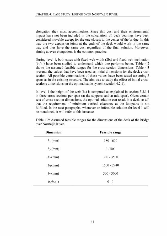
CHAPTER 4. CASE STUDY: BRIDGE OVER NORRTÄLJE RIVER
41
elongation they must accommodate. Since this cost and their environmental impact have not been included in the calculation, all deck bearings have been considered movable except for the one closest to the center of the bridge. In this way the two expansion joints at the ends of the deck would work in the same way and thus have the same cost regardless of the final solution. Moreover, aiming at even elongations is the common practice. During level 1, both cases with fixed web width (2b1) and fixed web inclination (b2/h1) have been studied to understand which one performs better. Table 4.2 shows the assumed feasible ranges for the cross-section dimensions. Table 4.3 presents the values that have been used as initial dimensions for the deck cross-section. All possible combinations of these values have been tested assuming 5 spans as in the existing structure. The aim was to study the effect of initial cross-sections dimensions on the optimal static system (section 4.2.1). In level 1 the height of the web (h1) is computed as explained in section 3.3.1.1 in three cross-sections per span (at the supports and at mid-span). Given certain sets of cross-section dimensions, the optimal solution can result in a deck so tall that the requirement of minimum vertical clearance at the footpaths is not fulfilled. In the next paragraphs, whenever an infeasible solution for level 1 will be mentioned, it will refer to this instance.
Table 4.2: Assumed feasible ranges for the dimensions of the deck of the bridge over Norrtälje River.
Dimension Feasible range
h3 (mm) 180 - 600
h2 (mm) 0 - 500
h1 (mm) 300 - 3500
b3 (mm) 1500 - 2940
b1 (mm) 500 - 3000
b2/h1 (-) 0 - 1
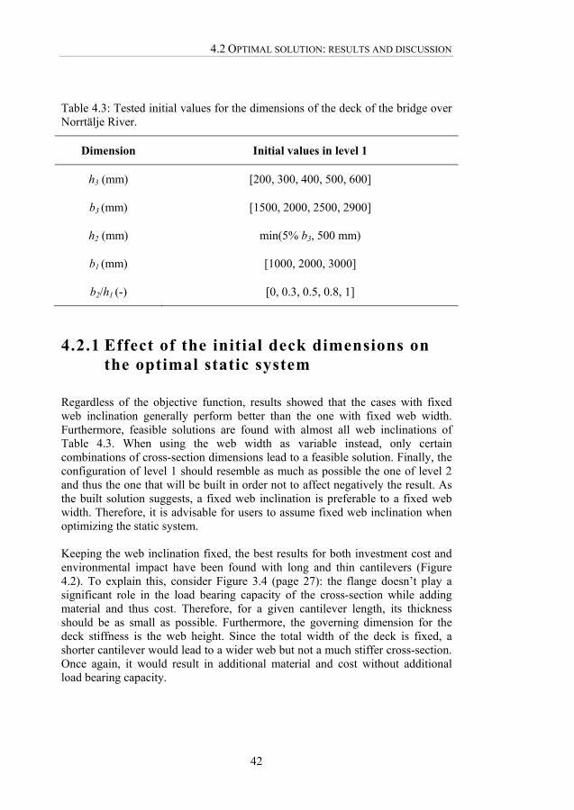
4.2 OPTIMAL SOLUTION: RESULTS AND DISCUSSION
42
Table 4.3: Tested initial values for the dimensions of the deck of the bridge over Norrtälje River.
Dimension Initial values in level 1
h3 (mm) [200, 300, 400, 500, 600]
b3 (mm) [1500, 2000, 2500, 2900]
h2 (mm) min(5% b3, 500 mm)
b1 (mm) [1000, 2000, 3000]
b2/h1 (-) [0, 0.3, 0.5, 0.8, 1]
4.2.1 Effect of the initial deck dimensions on the optimal static system
Regardless of the objective function, results showed that the cases with fixed web inclination generally perform better than the one with fixed web width. Furthermore, feasible solutions are found with almost all web inclinations of Table 4.3. When using the web width as variable instead, only certain combinations of cross-section dimensions lead to a feasible solution. Finally, the configuration of level 1 should resemble as much as possible the one of level 2 and thus the one that will be built in order not to affect negatively the result. As the built solution suggests, a fixed web inclination is preferable to a fixed web width. Therefore, it is advisable for users to assume fixed web inclination when optimizing the static system. Keeping the web inclination fixed, the best results for both investment cost and environmental impact have been found with long and thin cantilevers (Figure 4.2). To explain this, consider Figure 3.4 (page 27): the flange doesn’t play a significant role in the load bearing capacity of the cross-section while adding material and thus cost. Therefore, for a given cantilever length, its thickness should be as small as possible. Furthermore, the governing dimension for the deck stiffness is the web height. Since the total width of the deck is fixed, a shorter cantilever would lead to a wider web but not a much stiffer cross-section. Once again, it would result in additional material and cost without additional load bearing capacity.
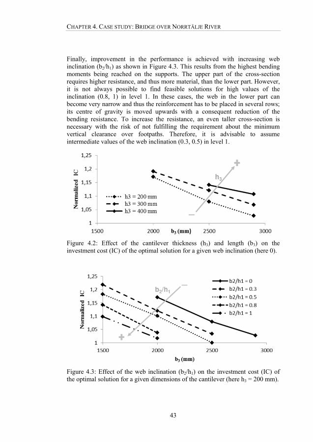
CHAPTER 4. CASE STUDY: BRIDGE OVER NORRTÄLJE RIVER
43
Finally, improvement in the performance is achieved with increasing web inclination (b2/h1) as shown in Figure 4.3. This results from the highest bending moments being reached on the supports. The upper part of the cross-section requires higher resistance, and thus more material, than the lower part. However, it is not always possible to find feasible solutions for high values of the inclination (0.8, 1) in level 1. In these cases, the web in the lower part can become very narrow and thus the reinforcement has to be placed in several rows; its centre of gravity is moved upwards with a consequent reduction of the bending resistance. To increase the resistance, an even taller cross-section is necessary with the risk of not fulfilling the requirement about the minimum vertical clearance over footpaths. Therefore, it is advisable to assume intermediate values of the web inclination (0.3, 0.5) in level 1.
Figure 4.2: Effect of the cantilever thickness (h3) and length (b3) on the investment cost (IC) of the optimal solution for a given web inclination (here 0).
Figure 4.3: Effect of the web inclination (b2/h1) on the investment cost (IC) of the optimal solution for a given dimensions of the cantilever (here h3 = 200 mm).
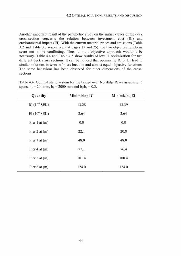
4.2 OPTIMAL SOLUTION: RESULTS AND DISCUSSION
44
Another important result of the parametric study on the initial values of the deck cross-section concerns the relation between investment cost (IC) and environmental impact (EI). With the current material prices and emissions (Table 3.2 and Table 3.7 respectively at pages 17 and 25), the two objective functions seem not to be conflicting. Thus, a multi-objective approach wouldn’t be necessary. Table 4.4 and Table 4.5 show results of level 1 optimization for two different deck cross sections. It can be noticed that optimizing IC or EI lead to similar solutions in terms of piers location and almost equal objective functions. The same behaviour has been observed for other dimensions of the cross-sections.
Table 4.4: Optimal static system for the bridge over Norrtälje River assuming: 5 spans, h3 = 200 mm, b3 = 2000 mm and b2/h1 = 0.3.
Quantity Minimizing IC Minimizing EI
IC (106 SEK) 13.28 13.39
EI (106 SEK) 2.64 2.64
Pier 1 at (m) 0.0 0.0
Pier 2 at (m) 22.1 20.8
Pier 3 at (m) 48.0 48.0
Pier 4 at (m) 77.1 76.4
Pier 5 at (m) 101.4 100.4
Pier 6 at (m) 124.0 124.0

CHAPTER 4. CASE STUDY: BRIDGE OVER NORRTÄLJE RIVER
45
Table 4.5: Optimal static system for the bridge over Norrtälje River assuming: 5 spans, h3 = 400 mm, b3 = 2500 mm and b2/h1 = 0.8.
Quantity Minimizing IC Minimizing EI
IC (106 SEK) 12.42 12.45
EI (106 SEK) 2.46 2.46
Pier 1 at (m) 0.0 0.0
Pier 2 at (m) 21.2 20.7
Pier 3 at (m) 48.1 48.0
Pier 4 at (m) 76.6 77.4
Pier 5 at (m) 102.9 103.3
Pier 6 at (m) 124.0 124.0
It is important to mention that values of IC and EI shown in this work are obtained as explained in sections 3.2.1 and 3.2.2. In particular, IC won’t be the actual total investment cost of the built solution since several contributions have not been considered (e.g. rent of machineries, cost of design etc.). Values of IC and EI shown in the tables should be treated as scores associated to solutions to allow ranking them. What matters the most are the relative differences/savings between solutions and not the absolute values. However, the way IC and EI have been formulated in this work makes them suitable objective functions for this optimization problem. Indeed, the neglected contributions won’t change significantly going from one solution to another; IC and EI here consider only what actually differentiates a solution from another in terms of material amount and buildability.
4.2.2 Optimal static system
Based on all considerations in section 4.2.1, the following values have been assumed for the initial deck cross-section: h3 = 200 mm, b3 = 2500 mm and b2/h1 = 0.5. Three possible configurations have been studied for level 1: 4, 5 and 6

4.2 OPTIMAL SOLUTION: RESULTS AND DISCUSSION
46
spans. The optimization has been performed twice: once minimizing EI and once minimizing IC. No feasible solutions have been found for 4 spans in both cases. Concerning the cases with 5 and 6 spans, results are summarized in Table 4.6 and Table 4.7. For the specific case study, the difference in terms of EI and IC for the cases with 5 and 6 spans isn’t significant (0.2 - 0.3%); therefore, the user can decide which static system to use in level 2 based on other criteria. In the presented work, the case with 5 spans has been selected. From the esthetical point of view, a more symmetric static system has been considered more pleasant. Considering the case that minimizes EI, indeed, the span lengths for the configurations with 5 and 6 spans are respectively 22.1 + 25.8 + 28.4 + 26 + 21.7 m and 15.7 + 14.5 + 18 + 27.8 + 25.4 + 22.6 m. Moreover, this choice allows for a more fair comparison with the built solution that presents 5 spans. Once again, referring to Table 4.6 and Table 4.7, IC and EI are not conflicting in the current case study: minimizing one leads to a low value of the other as well. It can also be noticed that the solution that minimize EI in the case with 6 spans reach lower values of IC than that minimizing IC itself. However, the difference is not significant (0.4%).
Table 4.6: Optimal static system for the bridge over Norrtälje River assuming: 5 spans, h3 = 200 mm, b3 = 2500 mm and b2/h1 = 0.5.
Quantity Minimizing IC Minimizing EI
IC (106 SEK) 11.99 12.00
EI (106 SEK) 2.32 2.32
Pier 1 at (m) 0.0 0.0
Pier 2 at (m) 22.0 22.1
Pier 3 at (m) 48.0 47.9
Pier 4 at (m) 76.3 76.3
Pier 5 at (m) 101.2 102.3
Pier 6 at (m) 124.0 124.0
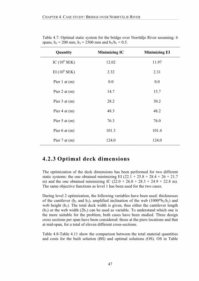
CHAPTER 4. CASE STUDY: BRIDGE OVER NORRTÄLJE RIVER
47
Table 4.7: Optimal static system for the bridge over Norrtälje River assuming: 6 spans, h3 = 200 mm, b3 = 2500 mm and b2/h1 = 0.5.
Quantity Minimizing IC Minimizing EI
IC (106 SEK) 12.02 11.97
EI (106 SEK) 2.32 2.31
Pier 1 at (m) 0.0 0.0
Pier 2 at (m) 14.7 15.7
Pier 3 at (m) 28.2 30.2
Pier 4 at (m) 48.3 48.2
Pier 5 at (m) 76.3 76.0
Pier 6 at (m) 101.3 101.4
Pier 7 at (m) 124.0 124.0
4.2.3 Optimal deck dimensions
The optimization of the deck dimensions has been performed for two different static systems: the one obtained minimizing EI (22.1 + 25.8 + 28.4 + 26 + 21.7 m) and the one obtained minimizing IC (22.0 + 26.0 + 28.3 + 24.9 + 22.8 m). The same objective functions as level 1 has been used for the two cases. During level 2 optimization, the following variables have been used: thicknesses of the cantilever (h2 and h3), amplified inclination of the web (1000*b2/h1) and web height (h1). The total deck width is given, thus either the cantilever length (b3) or the web width (2b1) can be used as variable. To understand which one is the more suitable for the problem, both cases have been studied. Three design cross sections per span have been considered: those at the piers locations and that at mid-span, for a total of eleven different cross-sections. Table 4.8-Table 4.11 show the comparison between the total material quantities and costs for the built solution (BS) and optimal solutions (OS). OS in Table

4.2 OPTIMAL SOLUTION: RESULTS AND DISCUSSION
48
4.10 and Table 4.11 are obtained minimizing EI, while in Table 4.8 and Table 4.9 minimizing IC. The optimization procedure applied to find OS in Table 4.8 and Table 4.10 used 2b1 as design variable, while that to find OS in Table 4.9 and Table 4.11 used b3. Eleven cross-sections have been considered with five design variables each for a total of 55 variables. For the sake of brevity, the obtained dimensions of the deck cross-sections are summarized in Table 4.12-Table 4.15. Once again, the two quantities used as objective functions appear not to be conflicting. Regardless of the used design variable and the objective function, a reduction of 8-15% on both IC and EI is obtained (Table 4.8-Table 4.11). Regarding the cross-section dimensions, all cases show big variations in the web height as expected for a continuous beam. However, the cases with 2b1 as design variable (Table 4.12 and Table 4.14), present shorter sections at the supports (i.e. lower maximum values of h1). Concerning the cantilever, all cases tend to make it as slender as possible as expected for the same reasons explained in section 4.2.1. However, the cases with 2b1 as design variable (Table 4.12 and Table 4.14), have longer cantilever than the others and thus steeper web inclinations (i.e. lower values). The consequence of these differences is that the performance of the optimization process with b3 (Table 4.9 and Table 4.11) as variable is slightly better. The geometric differences listed above have an effect on the savings in terms of materials. It can be noticed that high savings in the reinforcement amount (~20% in Table 4.9 and Table 4.11) correspond to high saving in both EI and IC. When the reinforcement amount is slightly increased in order to reduce the concrete (Table 4.8), IC gets slightly higher, while EI lower. However, if the increase in the reinforcement amount is significant, despite of a significant reduction of concrete (Table 4.10), the performance is poorer. These results are a first hint of the fact that the optimization is mainly led by the reinforcement amount regardless of the objective function. However, IC is more sensitive to changes in reinforcement amount than EI, while the latter is more sensitive to changes in concrete amount.
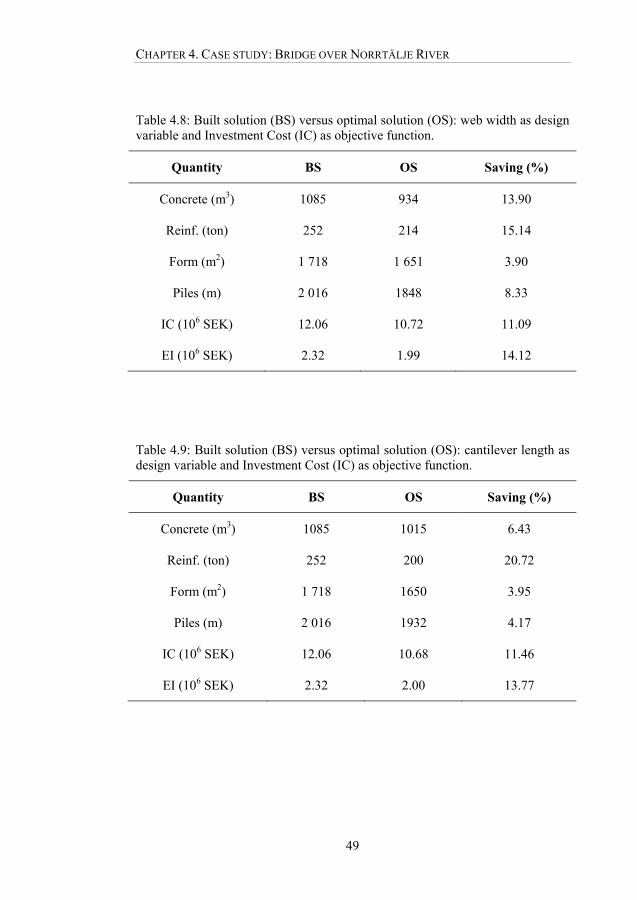
CHAPTER 4. CASE STUDY: BRIDGE OVER NORRTÄLJE RIVER
49
Table 4.8: Built solution (BS) versus optimal solution (OS): web width as design variable and Investment Cost (IC) as objective function.
Quantity BS OS Saving (%)
Concrete (m3) 1085 934 13.90
Reinf. (ton) 252 214 15.14
Form (m2) 1 718 1 651 3.90
Piles (m) 2 016 1848 8.33
IC (106 SEK) 12.06 10.72 11.09
EI (106 SEK) 2.32 1.99 14.12
Table 4.9: Built solution (BS) versus optimal solution (OS): cantilever length as design variable and Investment Cost (IC) as objective function.
Quantity BS OS Saving (%)
Concrete (m3) 1085 1015 6.43
Reinf. (ton) 252 200 20.72
Form (m2) 1 718 1650 3.95
Piles (m) 2 016 1932 4.17
IC (106 SEK) 12.06 10.68 11.46
EI (106 SEK) 2.32 2.00 13.77

4.2 OPTIMAL SOLUTION: RESULTS AND DISCUSSION
50
Table 4.10: Built solution (BS) versus optimal solution (OS): web width as design variable and Environmental Impact (EI) as objective function.
Quantity BS OS Saving (%)
Concrete (m3) 1085 901 16.91
Reinf. (ton) 252 230 8.61
Form (m2) 1 718 1 663 3.18
Piles (m) 2 016 1 848 8.33
IC (106 SEK) 12.06 11.02 8.65
EI (106 SEK) 2.32 2.05 11.87
Table 4.11: Built solution (BS) versus optimal solution (OS): cantilever length as design variable and Environmental Impact (EI) as objective function.
Quantity BS OS Saving (%)
Concrete (m3) 1085 1010 6.86
Reinf. (ton) 252 201 20.37
Form (m2) 1 718 1656 3.62
Piles (m) 2 016 2016 0.00
IC (106 SEK) 12.06 10.74 10.92
EI (106 SEK) 2.32 2.01 13.43
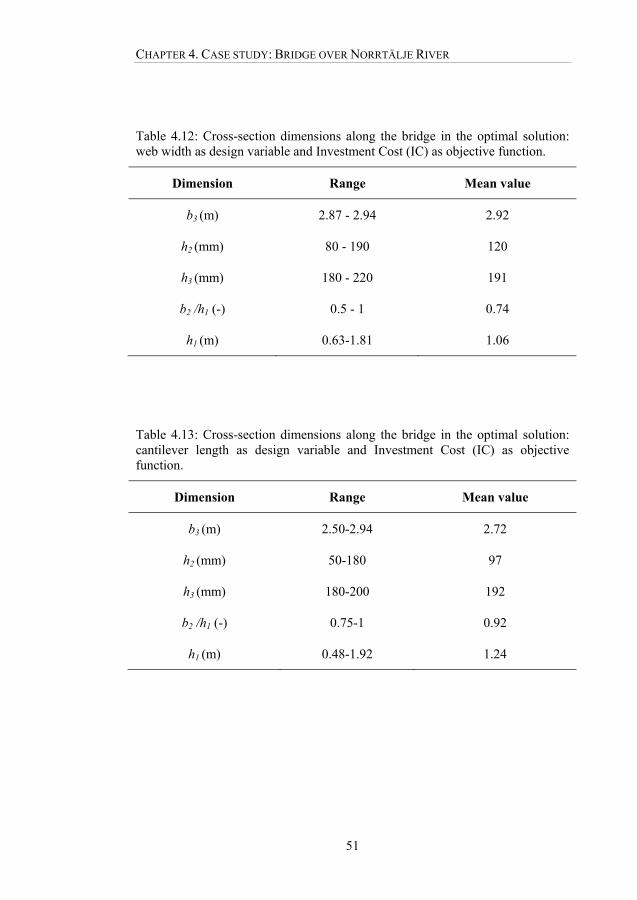
CHAPTER 4. CASE STUDY: BRIDGE OVER NORRTÄLJE RIVER
51
Table 4.12: Cross-section dimensions along the bridge in the optimal solution: web width as design variable and Investment Cost (IC) as objective function.
Dimension Range Mean value
b3 (m) 2.87 - 2.94 2.92
h2 (mm) 80 - 190 120
h3 (mm) 180 - 220 191
b2 /h1 (-) 0.5 - 1 0.74
h1 (m) 0.63-1.81 1.06
Table 4.13: Cross-section dimensions along the bridge in the optimal solution: cantilever length as design variable and Investment Cost (IC) as objective function.
Dimension Range Mean value
b3 (m) 2.50-2.94 2.72
h2 (mm) 50-180 97
h3 (mm) 180-200 192
b2 /h1 (-) 0.75-1 0.92
h1 (m) 0.48-1.92 1.24

4.2 OPTIMAL SOLUTION: RESULTS AND DISCUSSION
52
Table 4.14: Cross-section dimensions in the optimal solution: web width as design variable and Environmental Impact (EI) as objective function.
Dimension Range Mean value
b3 (m) 2.88 - 2.94 2.93
h2 (mm) 20 - 140 95
h3 (mm) 180 - 260 199
b2 /h1 (-) 0 – 0.93 0.52
h1 (m) 0.48-1.67 0.97
Table 4.15: Cross-section dimensions in the optimal solution: cantilever length as design variable and Environmental Impact (EI) as objective function.
Dimension Range Mean value
b3 (m) 2.50-2.93 2.73
h2 (mm) 50-130 80
h3 (mm) 180-230 199
b2 /h1 (-) 0.78-1 0.91
h1 (m) 0.51-1.92 1.22

CHAPTER 4. CASE STUDY: BRIDGE OVER NORRTÄLJE RIVER
53
Consider now the optimal solution obtained minimizing EI and using as design variable the cantilever length. Figure 4.4 shows the variation of the amount of building materials, EI and IC during the optimization process. The vertical line represents the passage from level 1 to level 2, which needs many more generations (i.e. iterations) to find the optimal solution due to the higher number of variables. All quantities are normalized with respect to the corresponding values in the first feasible solution. The trends of the investment cost and the environmental impact are similar, thus confirming the idea that the two objective functions are not conflicting.
Figure 4.4: Variation of the amount of building materials, EI and IC during the optimization. The vertical line represents the passage from level 1 to level 2.
The considerations about the relationships between materials amount and objective functions of section 4.2.3 meet the results in Figure 4.4 and Figure 4.5. In some portions of the first graph, the environmental impact shows a slightly stronger dependence on the concrete amount than the investment cost. Such result is confirmed by Figure 4.5 that shows the materials contribution on EI and IC for the optimal solution. Since IC includes the form and scaffolding, while EI doesn’t, a modified IC that considers only concrete, reinforcement and RC piles has been computed. In this way the comparison between IC and EI in terms of materials contributions is easier. The graphs of Figure 4.5 clearly show that concrete has a higher impact on EI than it has on IC. However, reinforcement contributes the most to both IC and EI.
0 20 40 60 80 100 120 140 160 180 200Generations
0.8
0.85
0.9
0.95
1
1.05
Nor
mal
ized
qua
ntit
ies
Optimizing the Environmental impact
Investment CostEnvironment CostConcrete volumeSteel massForm workpile length

4.2 OPTIMAL SOLUTION: RESULTS AND DISCUSSION
54
Finally, concerning the impact categories, Figure 4.6 shows that the highest contribution to the total environmental impact comes from the global warming as expected (section 3.2.2).
Figure 4.5: Materials contributions to the total environmental impact, the total investment cost and the modified investment cost (i.e. investment cost of only concrete, reinforcement and RC piles).
Figure 4.6: Impact categories contributions to the total environmental impact.
4.2.4 Effect of initial mesh size on the deck dimensions
Referring to the description of the Pattern Search (PS) algorithm in section 3.4.2.1, it is easy to understand that the result of such a deterministic search is affected by the starting point and the initial mesh size. In the current application, the starting point is represented by the dimensions of all cross-sections at the end of level one. Most of them have been pre-assigned as described in section 4.2.1, while the web height is the result of the design procedure of section 3.3.1.1. Concerning the initial mesh size, a value equal to 150 has been used to obtain all the solutions shown up to now. A sensitivity analysis considering three different values for the initial mesh size (0.0150, 1.5, 150) has been performed considering EI as objective function and using the cantilever length as design variable. The complete solutions in terms of design variables are shown in Figure

CHAPTER 4. CASE STUDY: BRIDGE OVER NORRTÄLJE RIVER
55
4.7-Figure 4.9 and Table 4.16, Table 4.18 and Table 4.20, while the comparison with the built solution in Table 4.17, Table 4.19 and Table 4.21. In terms of number of iterations required to reach the optimum, these values are 227, 293 and 185 for mesh sizes 0.0150, 1.5 and 150 respectively.
It can be observed that higher savings have been achieved with smaller initial mesh sizes. Concerning the web inclination and the cantilever dimensions, the three solutions don’t differ too much: they all point towards long and thin cantilever and high web inclination (i.e. almost 45º). Concerning the distribution of web heights long the deck. All the solutions show:
Almost constant height in the first and last half spans, Taller cross sections at the bearings than in the field, Almost symmetrical cross-sections in each span, except for the first and
the last one. However, there are some significant differences between the h1 values for the case with lowest savings (i.e. that with initial mesh size equal to 150) and the other two: Better results are obtained when:
The cross-sections are symmetric not only in each span but also with respect to the center of the bridge.
The height of the cross-section at the two central piers is reduces to match that at the other supports.
To conclude, the initial mesh size plays an important role in the level 2 optimization. The design variables in this case study were of the order of magnitude 103 (b3 and h1) and 102 (h2, h3 and 1000b2/h1). The optimizations with the best results have been obtained with initial mesh sizes much smaller than the variables (at least two orders of magnitude). However, it is not possible to draw a general conclusion since only one case study has been analyzed: further researches are required for determining the optimal initial mesh size applicable to other case studies.

4.2 OPTIMAL SOLUTION: RESULTS AND DISCUSSION
56
Span 1: length 22.100 m b1: 1000 b2: 1100 b3: 2900 h1: 1110 h2: 90 h3: 200 b1: 1001 b2: 1079 b3: 2920 h1: 1080 h2: 80 h3: 200 b1: 1002 b2: 1498 b3: 2500 h1: 1720 h2: 60 h3: 190 Intermediate pier 1: movable bearing Span 2: length 25.800 m b1: 1002 b2: 1498 b3: 2500 h1: 1720 h2: 60 h3: 190 b1: 1507 b2: 693 b3: 2800 h1: 700 h2: 70 h3: 200 b1: 1004 b2: 1496 b3: 2500 h1: 1870 h2: 50 h3: 200 Intermediate pier 2: fixed bearing Span 3: length 28.400 m b1: 1004 b2: 1496 b3: 2500 h1: 1870 h2: 50 h3: 200 b1: 1088 b2: 982 b3: 2930 h1: 1180 h2: 80 h3: 200 b1: 1000 b2: 1500 b3: 2500 h1: 1910 h2: 60 h3: 190 Intermediate pier 3: movable bearing Span 4: length 26.000 m b1: 1000 b2: 1500 b3: 2500 h1: 1910 h2: 60 h3: 190 b1: 1457 b2: 773 b3: 2770 h1: 780 h2: 130 h3: 180 b1: 1001 b2: 1499 b3: 2500 h1: 1920 h2: 50 h3: 230 Intermediate pier 4: movable bearing Span 5: length 21.700 m b1: 1001 b2: 1499 b3: 2500 h1: 1920 h2: 50 h3: 230 b1: 1591 b2: 509 b3: 2900 h1: 510 h2: 80 h3: 200 b1: 1607 b2: 603 b3: 2790 h1: 650 h2: 130 h3: 200
Figure 4.7: Optimal solution: Environmental Impact (EI) as objectivefunction and initial mesh size 150.
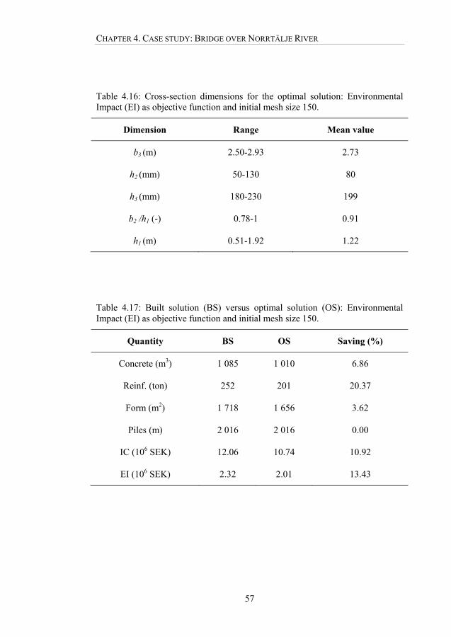
CHAPTER 4. CASE STUDY: BRIDGE OVER NORRTÄLJE RIVER
57
Table 4.16: Cross-section dimensions for the optimal solution: Environmental Impact (EI) as objective function and initial mesh size 150.
Dimension Range Mean value
b3 (m) 2.50-2.93 2.73
h2 (mm) 50-130 80
h3 (mm) 180-230 199
b2 /h1 (-) 0.78-1 0.91
h1 (m) 0.51-1.92 1.22
Table 4.17: Built solution (BS) versus optimal solution (OS): Environmental Impact (EI) as objective function and initial mesh size 150.
Quantity BS OS Saving (%)
Concrete (m3) 1 085 1 010 6.86
Reinf. (ton) 252 201 20.37
Form (m2) 1 718 1 656 3.62
Piles (m) 2 016 2 016 0.00
IC (106 SEK) 12.06 10.74 10.92
EI (106 SEK) 2.32 2.01 13.43
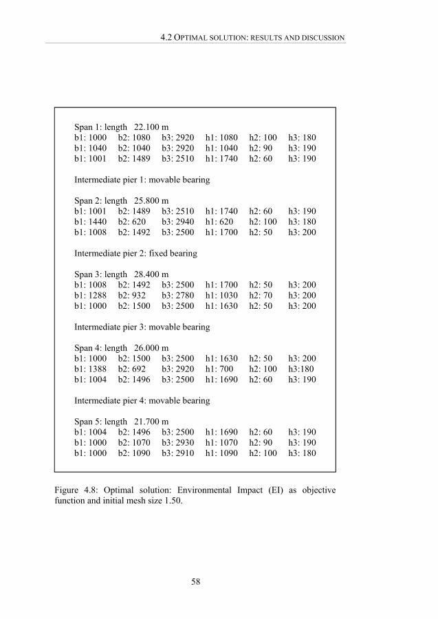
4.2 OPTIMAL SOLUTION: RESULTS AND DISCUSSION
58
Span 1: length 22.100 m b1: 1000 b2: 1080 b3: 2920 h1: 1080 h2: 100 h3: 180 b1: 1040 b2: 1040 b3: 2920 h1: 1040 h2: 90 h3: 190 b1: 1001 b2: 1489 b3: 2510 h1: 1740 h2: 60 h3: 190 Intermediate pier 1: movable bearing Span 2: length 25.800 m b1: 1001 b2: 1489 b3: 2510 h1: 1740 h2: 60 h3: 190 b1: 1440 b2: 620 b3: 2940 h1: 620 h2: 100 h3: 180 b1: 1008 b2: 1492 b3: 2500 h1: 1700 h2: 50 h3: 200 Intermediate pier 2: fixed bearing Span 3: length 28.400 m b1: 1008 b2: 1492 b3: 2500 h1: 1700 h2: 50 h3: 200 b1: 1288 b2: 932 b3: 2780 h1: 1030 h2: 70 h3: 200 b1: 1000 b2: 1500 b3: 2500 h1: 1630 h2: 50 h3: 200 Intermediate pier 3: movable bearing Span 4: length 26.000 m b1: 1000 b2: 1500 b3: 2500 h1: 1630 h2: 50 h3: 200 b1: 1388 b2: 692 b3: 2920 h1: 700 h2: 100 h3:180 b1: 1004 b2: 1496 b3: 2500 h1: 1690 h2: 60 h3: 190 Intermediate pier 4: movable bearing Span 5: length 21.700 m b1: 1004 b2: 1496 b3: 2500 h1: 1690 h2: 60 h3: 190 b1: 1000 b2: 1070 b3: 2930 h1: 1070 h2: 90 h3: 190 b1: 1000 b2: 1090 b3: 2910 h1: 1090 h2: 100 h3: 180
Figure 4.8: Optimal solution: Environmental Impact (EI) as objectivefunction and initial mesh size 1.50.
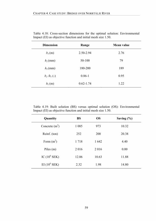
CHAPTER 4. CASE STUDY: BRIDGE OVER NORRTÄLJE RIVER
59
Table 4.18: Cross-section dimensions for the optimal solution: Environmental Impact (EI) as objective function and initial mesh size 1.50.
Dimension Range Mean value
b3 (m) 2.50-2.94 2.76
h2 (mm) 50-100 79
h3 (mm) 180-200 189
b2 /h1 (-) 0.86-1 0.95
h1 (m) 0.62-1.74 1.22
Table 4.19: Built solution (BS) versus optimal solution (OS): Environmental Impact (EI) as objective function and initial mesh size 1.50.
Quantity BS OS Saving (%)
Concrete (m3) 1 085 973 10.32
Reinf. (ton) 252 200 20.38
Form (m2) 1 718 1 642 4.40
Piles (m) 2 016 2 016 0.00
IC (106 SEK) 12.06 10.63 11.88
EI (106 SEK) 2.32 1.98 14.80

4.2 OPTIMAL SOLUTION: RESULTS AND DISCUSSION
60
Span 1: length 22.100 m b1: 1005 b2: 1055 b3: 2940 h1: 1090 h2: 90 h3: 200 b1: 1036 b2: 1124 b3: 2840 h1: 1140 h2: 80 h3: 190 b1: 1000 b2: 1500 b3: 2500 h1: 1610 h2: 60 h3: 240 Intermediate pier 1: movable bearing Span 2: length 25.800 m b1: 1000 b2: 1500 b3: 2500 h1: 1610 h2: 60 h3: 240 b1: 1393 b2: 667 b3: 2940 h1: 680 h2: 80 h3: 200 b1: 1026 b2: 1104 b3: 2870 h1: 1460 h2: 140 h3: 200 Intermediate pier 2: fixed bearing Span 3: length 28.400 m b1: 1026 b2: 1104 b3: 2870 h1: 1460 h2: 140 h3: 200 b1: 1038 b2: 1042 b3: 2920 h1: 1150 h2: 100 h3: 180 b1: 1002 b2: 1068 b3: 2930 h1: 1720 h2: 80 h3: 230 Intermediate pier 3: movable bearing Span 4: length 26.000 m b1: 1002 b2: 1068 b3: 2930 h1: 1720 h2: 80 h3: 230 b1: 1462 b2: 628 b3: 2910 h1: 630 h2: 80 h3: 200 b1: 1000 b2: 1500 b3: 2500 h1: 1550 h2: 60 h3: 190 Intermediate pier 4: movable bearing Span 5: length 21.700 m b1: 1000 b2: 1500 b3: 2500 h1: 1550 h2: 60 h3: 190 b1: 1038 b2: 1122 b3: 2840 h1: 1140 h2: 90 h3: 190 b1: 1000 b2: 1210 b3: 2790 h1: 1220 h2: 70 h3: 200
Figure 4.9: Optimal solution: Environmental Impact (EI) as objectivefunction and initial mesh size 0.0150.

CHAPTER 4. CASE STUDY: BRIDGE OVER NORRTÄLJE RIVER
61
Table 4.20: Cross-section dimensions for the optimal solution: Environmental Impact (EI) as objective function and initial mesh size 0.0150.
Dimension Range Mean value
b3 (m) 2.50-2.94 2.82
h2 (mm) 60-140 85
h3 (mm) 180-240 202
b2 /h1 (-) 0.62-1 0.92
h1 (m) 0.63-1.72 1.22
Table 4.21: Built solution (BS) versus optimal solution (OS): Environmental Impact (EI) as objective function and initial mesh size 0.0150.
Quantity BS OS Saving (%)
Concrete (m3) 1 085 970 10.44
Reinf. (ton) 252 199 21.11
Form (m2) 1 718 1 650 3.96
Piles (m) 2 016 2 016 0.00
IC (106 SEK) 12.06 10.60 12.09
EI (106 SEK) 2.32 1.97 15.23
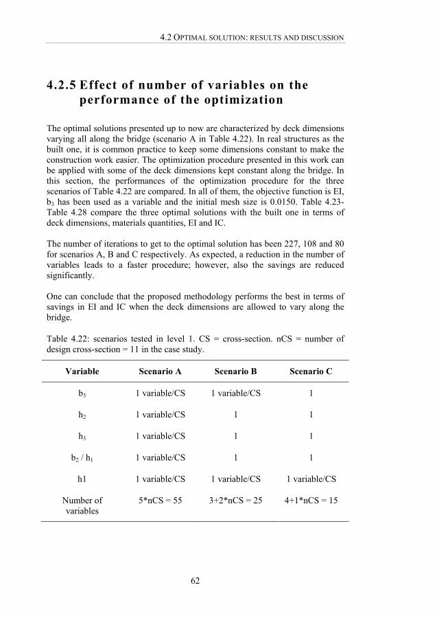
4.2 OPTIMAL SOLUTION: RESULTS AND DISCUSSION
62
4.2.5 Effect of number of variables on the performance of the optimization
The optimal solutions presented up to now are characterized by deck dimensions varying all along the bridge (scenario A in Table 4.22). In real structures as the built one, it is common practice to keep some dimensions constant to make the construction work easier. The optimization procedure presented in this work can be applied with some of the deck dimensions kept constant along the bridge. In this section, the performances of the optimization procedure for the three scenarios of Table 4.22 are compared. In all of them, the objective function is EI, b3 has been used as a variable and the initial mesh size is 0.0150. Table 4.23-Table 4.28 compare the three optimal solutions with the built one in terms of deck dimensions, materials quantities, EI and IC. The number of iterations to get to the optimal solution has been 227, 108 and 80 for scenarios A, B and C respectively. As expected, a reduction in the number of variables leads to a faster procedure; however, also the savings are reduced significantly. One can conclude that the proposed methodology performs the best in terms of savings in EI and IC when the deck dimensions are allowed to vary along the bridge.
Table 4.22: scenarios tested in level 1. CS = cross-section. nCS = number of design cross-section = 11 in the case study.
Variable Scenario A Scenario B Scenario C
b3 1 variable/CS 1 variable/CS 1
h2 1 variable/CS 1 1
h3 1 variable/CS 1 1
b2 / h1 1 variable/CS 1 1
h1 1 variable/CS 1 variable/CS 1 variable/CS
Number of variables
5*nCS = 55 3+2*nCS = 25 4+1*nCS = 15
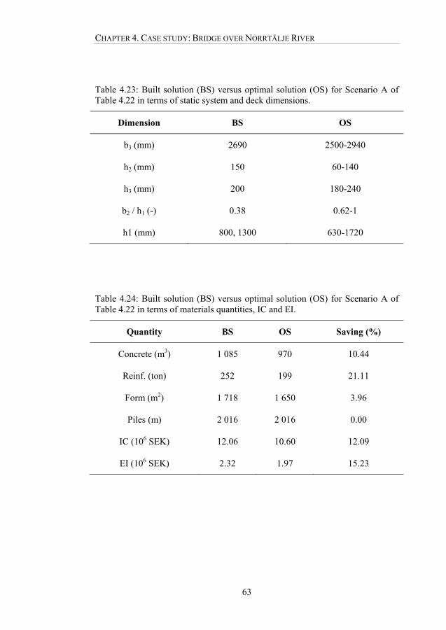
CHAPTER 4. CASE STUDY: BRIDGE OVER NORRTÄLJE RIVER
63
Table 4.23: Built solution (BS) versus optimal solution (OS) for Scenario A of Table 4.22 in terms of static system and deck dimensions.
Dimension BS OS
b3 (mm) 2690 2500-2940
h2 (mm) 150 60-140
h3 (mm) 200 180-240
b2 / h1 (-) 0.38 0.62-1
h1 (mm) 800, 1300 630-1720
Table 4.24: Built solution (BS) versus optimal solution (OS) for Scenario A of Table 4.22 in terms of materials quantities, IC and EI.
Quantity BS OS Saving (%)
Concrete (m3) 1 085 970 10.44
Reinf. (ton) 252 199 21.11
Form (m2) 1 718 1 650 3.96
Piles (m) 2 016 2 016 0.00
IC (106 SEK) 12.06 10.60 12.09
EI (106 SEK) 2.32 1.97 15.23

4.2 OPTIMAL SOLUTION: RESULTS AND DISCUSSION
64
Table 4.25: Built solution (BS) versus optimal solution (OS) for Scenario B of Table 4.22 in terms of static system and deck dimensions.
Dimension BS OS
b3 (mm) 2690 2500-2840
h2 (mm) 150 80
h3 (mm) 200 190
b2 / h1 (-) 0.38 0.75
h1 (mm) 800, 1300 650 - 1990
Table 4.26: Built solution (BS) versus optimal solution (OS) for Scenario B of Table 4.22 in terms of materials quantities, IC and EI.
Quantity BS OS Saving (%)
Concrete (m3) 1 085 997 8.10
Reinf. (ton) 252 207 17.95
Form (m2) 1 718 1 664 3.14
Piles (m) 2 016 2 016 0.00
IC (106 SEK) 12.06 10.85 10.01
EI (106 SEK) 2.32 2.03 12.64
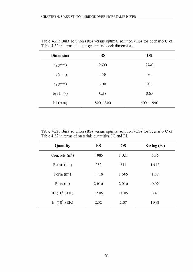
CHAPTER 4. CASE STUDY: BRIDGE OVER NORRTÄLJE RIVER
65
Table 4.27: Built solution (BS) versus optimal solution (OS) for Scenario C of Table 4.22 in terms of static system and deck dimensions.
Dimension BS OS
b3 (mm) 2690 2740
h2 (mm) 150 70
h3 (mm) 200 200
b2 / h1 (-) 0.38 0.63
h1 (mm) 800, 1300 600 - 1990
Table 4.28: Built solution (BS) versus optimal solution (OS) for Scenario C of Table 4.22 in terms of materials quantities, IC and EI.
Quantity BS OS Saving (%)
Concrete (m3) 1 085 1 021 5.86
Reinf. (ton) 252 211 16.15
Form (m2) 1 718 1 685 1.89
Piles (m) 2 016 2 016 0.00
IC (106 SEK) 12.06 11.05 8.41
EI (106 SEK) 2.32 2.07 10.81
4.2 OPTIMAL SOLUTION: RESULTS AND DISCUSSION
66
4.2.6 Easy-to-build optimal solutions
Instead of obtaining a solution more construction-friendly as shown in the previous section, it is possible to manually modify the optimal one obtained in Scenario A (Table 4.22). That solution is characterized by spans of various lengths and deck dimensions varying all along the bridge. A more buildable solution (Buildable Optimal Solution BOS) has been designed based on it. Concerning the static system, the aim was to have a symmetrical structure. The span lengths for BOS have been computed averaging the values of the optimal one. An accuracy of 0.5 m for the span lengths has been used to allow for an easier construction. Concerning the deck cross-section, the cantilever part and the web inclination have been kept constant as in the built solution, while the web height varies. The indications in section 4.2.4 have been followed. Moreover, it has been observed in Figure 4.9 that the field of the second and second to last spans required shorter cross-sections than the other spans. The comparison between the proposed Buildable Optimal Solution (BOS) and the built solution (BS) is presented in Table 4.29 and Table 4.30. The comparison in Table 4.29 shows that simply adjusting the spans lengths, increasing the deck height and web inclination and adding one design cross-section, gives savings of more than 10% both for EI and IC (Table 4.30). Such savings are possible without having to change the bridge type, the construction method, the material etc. The BOS designed in this way gives higher savings than the ones obtained by fixing some of the deck dimensions during the optimization (i.e. Scenarios B and C in Table 4.22). Thus, it is confirmed that the best use of the proposed design and optimization methodology consists in:
Assuming that all deck dimensions can vary along the bridge during the optimization process.
Manually adjust the optimal solution at the end to meet aesthetic and functional requirements.
The results presented in this section are very promising. Indeed, the Bridge over Norrtälje River has been designed by an experienced engineer, as similarities between BS and OS prove. If the application of the design procedure proposed in this work leads to savings of 10-15% for such a structure, even better results can be expected for other structures. Moreover, this procedure would allow engineers with limited experience to design optimal solutions saving materials and lowering the environmental impact.

CHAPTER 4. CASE STUDY: BRIDGE OVER NORRTÄLJE RIVER
67
Table 4.29: Built solution (BS) versus buildable optimal solution (BOS) in terms of static system and deck dimensions. MB = movable bearing, FB = fixed bearing.
Variable BS BOS
Spans lengths (m) 21.5 27 27 27 21.5 22 26 28 26 22
Bearings MB MB MB FB MB MB MB MB FB MB MB MB
b3 (mm) 2690 2750
h2 (mm) 150 100
h3 (mm) 200 180
b2 / h1 (-) 0.38 (i.e. h1 = 2.6·b2) 0.91 (i.e. h1 = 1.1·b2)
h1 (mm)
800: field of all spans
800: abutments
1300: intermediate supports
1100: field of spans 1-3-5 600: field of spans 2-4
1100: abutments
1700: intermediate supports
Table 4.30: Built solution (BS) versus buildable optimal solution (BOS) in terms of materials quantities, IC and EI.
Quantity BS BOS Saving (%)
Concrete (m3) 1 085 988 8.87
Reinf. (ton) 252 207 17.80
Form (m2) 1 718 1 677 2.37
Piles (m) 2 016 2 016 0.00
IC (106 SEK) 12.06 10.83 10.17
EI (106 SEK) 2.32 2.02 12.88

4.2 OPTIMAL SOLUTION: RESULTS AND DISCUSSION
68
4.2.7 Effect of reduced unit impacts of materials
Promising results have been obtained both for the investment cost and the environmental impact by slightly changing the dimensions of bridge. The next step consists of investigating the effect of a reduction in the unit emissions of materials. Concerning reinforcement, one way for reducing the impact is to increase the amount of recycled steel. Regarding concrete, cement producers could work on the used materials and on enhancing the manufacturing process. In this section, a fictitious reduction of 30% in the emissions of concrete and reinforcement has been applied separately. The two optimal solutions (minimizing EI) for the Bridge over Norrtälje River are compared. The aim is to identify in which direction research and industries should move concerning the reduction of emissions in the production phase. Table 4.31 compares the two optimal solutions. The one obtained assuming reduced emissions of steel leads to a more environmental friendly and cost effective solution compared to the solution obtained assuming reduced emissions of concrete. However, it presents a higher content of reinforcement. This result is reasonable: reducing the unit emission of reinforcement makes the concrete a bigger problem for the environmental impact. As a consequence, the optimization procedure tries to minimize the concrete amount thus increasing the reinforcement amount. This idea gets clearer looking at Table 4.32 and Table 4.33. They present the comparison between the optimal solutions (OS) with reduced impacts and the built one. For a fair comparison, EI for the built solution (BS) has been re-computed assuming reduced emissions of materials. In the case with reduced unit emission of concrete, the optimization tends to focus on reducing the reinforcement amount. On the other hand, when producing reinforcement gets more environmental-friendly, the reductions are moved towards concrete amount as well. Furthermore, by reducing the unit emissions associated with reinforcement production, EI for the built solution decreases. To conclude, one can say that a reduction in the unit emissions of reinforcement would be more beneficial than the same reduction in the unit emission of concrete.

CHAPTER 4. CASE STUDY: BRIDGE OVER NORRTÄLJE RIVER
69
Table 4.31: Comparison between the optimal solutions obtained reducing the unit emissions of concrete and reinforcement.
Quantity Reducing concrete unit emission by
30%
Reducing steel unit emission by
30%
Difference
(%)
Concrete (m3) 1 032 931 10.33
Reinf. (ton) 198 209 -5.40
Form (m2) 1 695 1 635 3.53
Piles (m) 2 016 1 932 4.17
IC
(106 SEK) 10.79 10.64 1.40
EI
(106 SEK) 1.75 1.67 4.73
Table 4.32: Built solution (BS) versus optimal solution (OS) with reduced concrete unit emission by 30%.
Quantity BS OS Saving (%)
Concrete (m3) 1 085 1 032 4.87
Reinf. (ton) 252 198 21.30
Form (m2) 1 718 1 695 1.34
Piles (m) 2 016 2 016 0.00
IC (106 SEK) 12.06 10.79 10.53
EI (106 SEK) 2.05 1.75 14.24

4.2 OPTIMAL SOLUTION: RESULTS AND DISCUSSION
70
Table 4.33: Built solution (BS) versus optimal solution (OS) with reduced steel unit emission by 30%.
Quantity BS OS Saving (%)
Concrete (m3) 1 085 931 14.21
Reinf. (ton) 252 209 17.05
Form (m2) 1 718 1 635 4.82
Piles (m) 2 016 1 932 4.17
IC (106 SEK) 12.06 10.64 11.78
EI (106 SEK) 1.96 1.67 14.52

71
5 Parametric studies
Chapter 4 showed the potential of replacing the current design practice with the use of the developed software in one case study. In this chapter, a further step is done: the design and optimization procedure is applied to several cases in order to draw general conclusions and produce guidelines for designers.
5.1 Optimal number of spans
As previously explained, level 1 aims to find the optimal static system including the optimal number of spans. To do so, the optimization of the static system is performed as many times as the number of different configurations (i.e. number of spans) the user wants to test. The configuration corresponding to the lowest value of the objective function is then used during level 2. The graphs in Figure 5.1 and Figure 5.2 are obtained by performing level 1 optimization on a set of total bridge lengths. As in the case of the Bridge over Norrtälje River, the deck cross-section has been assumed to have constant width of 10 m. Moreover, the following values have been assumed for the other deck dimensions: h3 = 200 mm, b3 = 2500 mm and b2/h1 = 0.5. The distance between the deck upper surface and the ground level has been assumed to be constant all along the bridge and equal to 5 m. A minimum clearance of 3 m all along the bridge has been assumed as well. No infeasible regions for the piers have been considered and only numbers of spans which allowed for spans length in the range 8-404 m have
4 For spans longer than 40 m prestressed decks are usually used.
Chapter
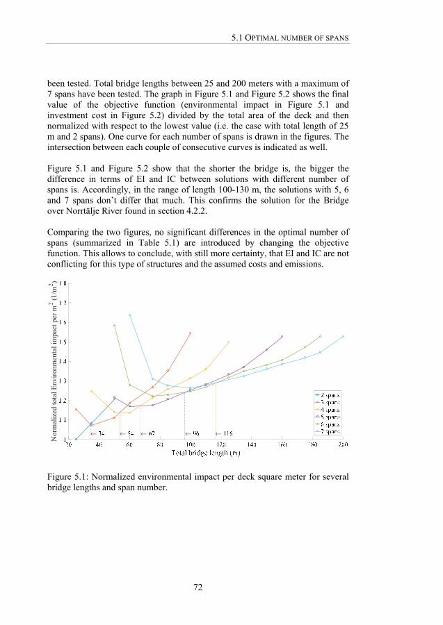
5.1 OPTIMAL NUMBER OF SPANS
72
been tested. Total bridge lengths between 25 and 200 meters with a maximum of 7 spans have been tested. The graph in Figure 5.1 and Figure 5.2 shows the final value of the objective function (environmental impact in Figure 5.1 and investment cost in Figure 5.2) divided by the total area of the deck and then normalized with respect to the lowest value (i.e. the case with total length of 25 m and 2 spans). One curve for each number of spans is drawn in the figures. The intersection between each couple of consecutive curves is indicated as well. Figure 5.1 and Figure 5.2 show that the shorter the bridge is, the bigger the difference in terms of EI and IC between solutions with different number of spans is. Accordingly, in the range of length 100-130 m, the solutions with 5, 6 and 7 spans don’t differ that much. This confirms the solution for the Bridge over Norrtälje River found in section 4.2.2. Comparing the two figures, no significant differences in the optimal number of spans (summarized in Table 5.1) are introduced by changing the objective function. This allows to conclude, with still more certainty, that EI and IC are not conflicting for this type of structures and the assumed costs and emissions.
Figure 5.1: Normalized environmental impact per deck square meter for several bridge lengths and span number.
Nor
mal
ized
tota
l Env
iron
men
tal i
mpa
ct p
er m
2 (1/
m2 )

CHAPTER 5. PARAMETRIC STUDIES
73
Figure 5.2: Normalized investment cost per deck square meter for several bridge lengths and span number.
Table 5.1: Optimal number of spans to minimize the environmental impact and the investment cost per deck square meter.
Total bridge length (m) Optimal number of spans
25-35 2
35-55 3
55-65 4
65-95 5
95-130 5-6-7
130-200 ≥7
Nor
mal
ized
tota
l Inv
estm
ent c
ost p
er m
2 (1/
m2 )
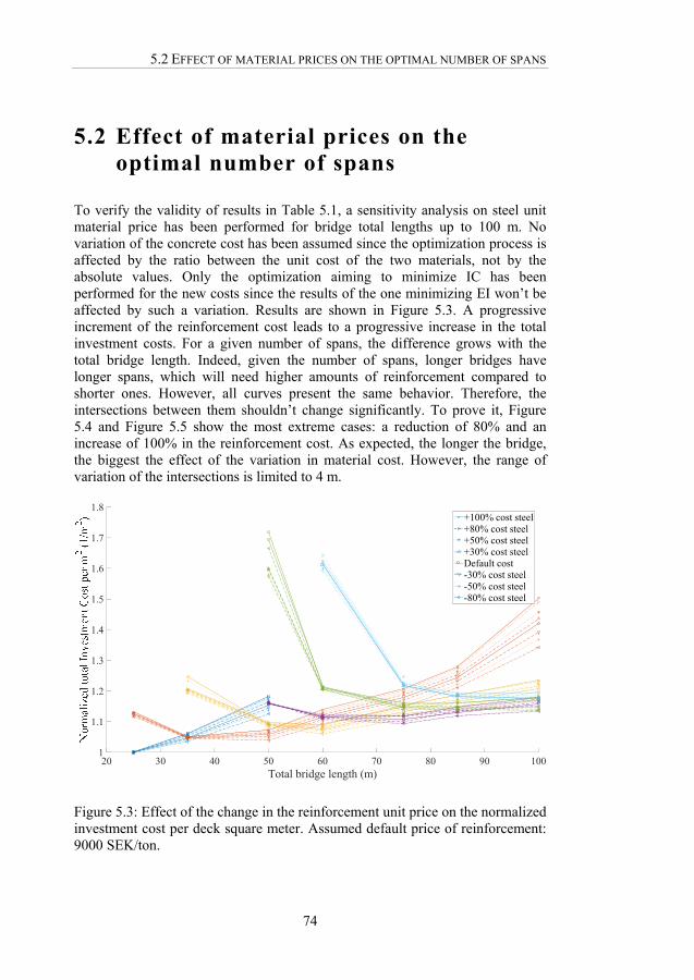
5.2 EFFECT OF MATERIAL PRICES ON THE OPTIMAL NUMBER OF SPANS
74
5.2 Effect of material prices on the optimal number of spans
To verify the validity of results in Table 5.1, a sensitivity analysis on steel unit material price has been performed for bridge total lengths up to 100 m. No variation of the concrete cost has been assumed since the optimization process is affected by the ratio between the unit cost of the two materials, not by the absolute values. Only the optimization aiming to minimize IC has been performed for the new costs since the results of the one minimizing EI won’t be affected by such a variation. Results are shown in Figure 5.3. A progressive increment of the reinforcement cost leads to a progressive increase in the total investment costs. For a given number of spans, the difference grows with the total bridge length. Indeed, given the number of spans, longer bridges have longer spans, which will need higher amounts of reinforcement compared to shorter ones. However, all curves present the same behavior. Therefore, the intersections between them shouldn’t change significantly. To prove it, Figure 5.4 and Figure 5.5 show the most extreme cases: a reduction of 80% and an increase of 100% in the reinforcement cost. As expected, the longer the bridge, the biggest the effect of the variation in material cost. However, the range of variation of the intersections is limited to 4 m.
Figure 5.3: Effect of the change in the reinforcement unit price on the normalized investment cost per deck square meter. Assumed default price of reinforcement: 9000 SEK/ton.
20 30 40 50 60 70 80 90 100Total bridge length (m)
1
1.1
1.2
1.3
1.4
1.5
1.6
1.7
1.8+100% cost steel+80% cost steel+50% cost steel+30% cost steelDefault cost-30% cost steel-50% cost steel-80% cost steel

CHAPTER 5. PARAMETRIC STUDIES
75
Figure 5.4: Normalized investment cost per deck square meter for several bridge lengths and span number. Assumed cost of reinforcement: 0.2*9000 SEK/ton.
Figure 5.5: Normalized investment cost per deck square meter for several bridge lengths and span number. Assumed cost of reinforcement: 2*9000 SEK/ton.
Nor
mal
ized
tota
l Inv
estm
ent c
ost p
er m
2 (1/
m2 )
Nor
mal
ized
tota
l Inv
estm
ent c
ost p
er m
2 (1/
m2 )

5.3 EFFECT OF UNIT EMISSIONS ON THE OPTIMAL NUMBER OF SPANS
76
To conclude, the concrete-steel price ratio has a small effect on the optimal number of spans and the indications of Table 5.1 are still valid in the length range 25-100 m.
5.3 Effect of unit emissions on the optimal number of spans
Concerning the optimization that uses as objective function EI, once again, results are affected by the ratio between the unit emissions of concrete and steel, not by the absolute values. However, instead of finding the optimal solutions increasing and then decreasing the emissions of only one material; the unit emissions of both have been dicreased saparately. In this way, two analysis can be performed. The first one aims, as in the case of IC, to analyze the sensitivity of results in Table 5.1 to the values assumed for the unit emissions. Such analysis is of major importance: unit emissions used in this work (Table 3.7 at page 25) are taken from the Ecoinvent v.2.01 (Ecoinvent, 2008) database that considers the typical European technologies and averages data collected in Europe and Worldwide. The single producer could use different technologies and thus give different values, which could lead to a different optimal configuration. Results of the sensitivity analysis are shown in Figure 5.6. Figure 5.7 and Figure 5.8 show the most extreme cases: a reduction of 50% in the reinforcement and concrete unit emissions. As in the previous section, the optimal number of spans isn’t strongly affected by these variations. Once again, the sensitivity increases for longer bridges. Thus, indications in Table 5.1 can still be used. The second type of analysis is similar to the one performed on the Bridge over Norrtälje River in section 4.2.7. It assumes values in Table 3.7 (i.e. taken from Ecoinvent v.2.01) as baseline and aims to understand which production technology should be improved in order to further reduce the environmental impact of this type of bridges. Referring to Figure 5.7 and Figure 5.8, given a total bridge length, all curves in the case of reduced concrete unit emission are higher than those with reduced reinforcement unit emission. In other words, a reduction in the unit emissions of reinforcement would be more beneficial for the environmental impact than the same reduction in the unit emission of concrete. This result confirms what has been found for the Bridge over Norrtälje River.
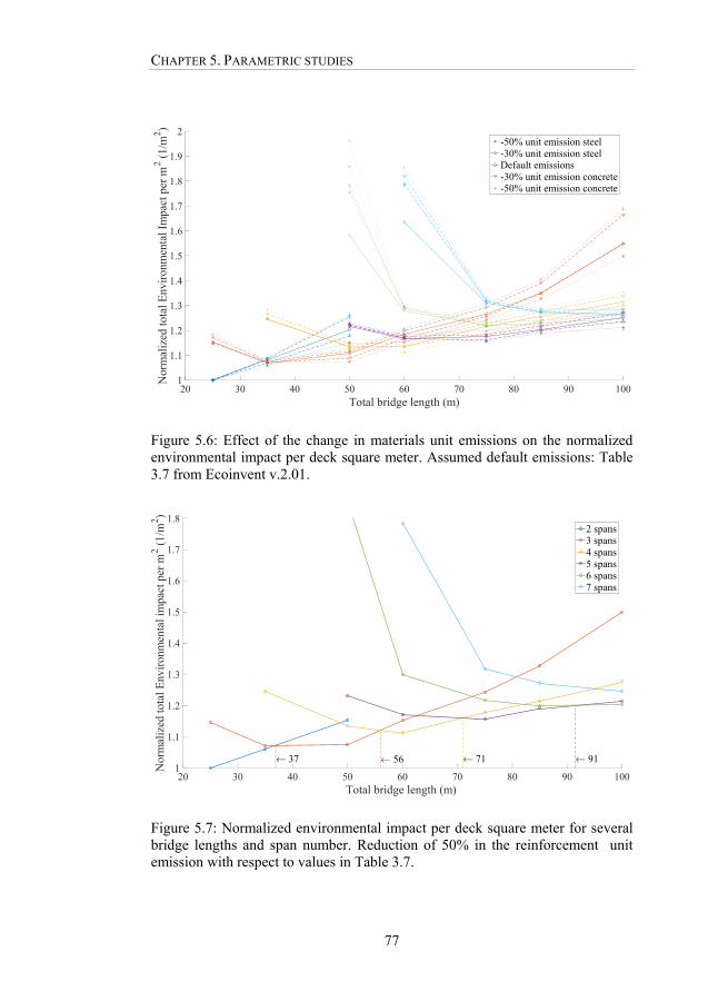
CHAPTER 5. PARAMETRIC STUDIES
77
Figure 5.6: Effect of the change in materials unit emissions on the normalized environmental impact per deck square meter. Assumed default emissions: Table 3.7 from Ecoinvent v.2.01.
Figure 5.7: Normalized environmental impact per deck square meter for several bridge lengths and span number. Reduction of 50% in the reinforcement unit emission with respect to values in Table 3.7.
20 30 40 50 60 70 80 90 100Total bridge length (m)
1
1.1
1.2
1.3
1.4
1.5
1.6
1.7
1.8
1.9
2
Nor
mal
ized
tota
l Env
iron
men
tal I
mpa
ct p
er m
2 (1/
m2 )
-50% unit emission steel-30% unit emission steelDefault emissions-30% unit emission concrete-50% unit emission concrete
20 30 40 50 60 70 80 90 100Total bridge length (m)
1
1.1
1.2
1.3
1.4
1.5
1.6
1.7
1.8
Nor
mal
ized
tota
l Env
iron
men
tal i
mpa
ct p
er m
2 (1/
m2 )
37 56 71 91
2 spans3 spans4 spans5 spans6 spans7 spans
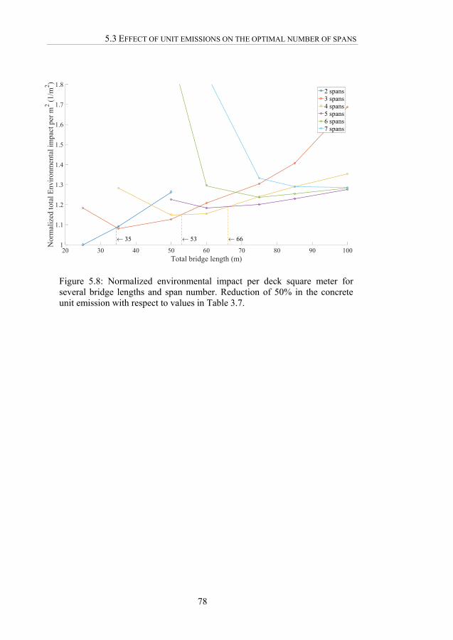
5.3 EFFECT OF UNIT EMISSIONS ON THE OPTIMAL NUMBER OF SPANS
78
Figure 5.8: Normalized environmental impact per deck square meter for several bridge lengths and span number. Reduction of 50% in the concrete unit emission with respect to values in Table 3.7.
20 30 40 50 60 70 80 90 100Total bridge length (m)
1
1.1
1.2
1.3
1.4
1.5
1.6
1.7
1.8
Nor
mal
ized
tota
l Env
iron
men
tal i
mpa
ct p
er m
2 (1/
m2 )
35 53 66
2 spans3 spans4 spans5 spans6 spans7 spans
79
6 Concluding remarks
In this chapter, the research work presented in this thesis is summarized, together with its main findings.
6.1 Conclusions
In this thesis, a two-steps automatic design and optimization procedure for RC road beam bridges has been presented. It finds the solution that minimizes the investment cost and the environmental impact of the bridge, while fulfilling all requirements of Eurocodes. In the first step, given the soil morphology and the two points to connect, it selects the optimal number of spans, type of piers-deck connections and piers location taking into account any obstacle the bridge has to cross. In the second and final step, it finds the optimal dimensions of the deck cross-sections. Furthermore, the required reinforcement for the deck is designed in a detailed way: given the bars diameters, spacing and cover, the total amount of bars and the exact layout are computed. A software for the application of the proposed procedure has been developed in MATLAB® and integrated with a commercial FEM software for the structural analysis of bridges. An application for the detailed design of reinforcement in RC sections has been developed as well. Pattern Search provided in MATLAB® Optimization Toolbox has been used as optimization algorithms together with a modified version of Genetic Algorithm. A memory system has been integrated to make the process faster and treat continuous variables in a discrete way.
Chapter
6.1 CONCLUSIONS
80
The software has been tested on an existing bridge recently designed according to Eurocodes standards. Several analyses have been carried out in this case study leading to the following results.
The performance of the optimization procedure is affected by the user
choices in terms of number and type of variables, initial dimensions and parameters used by the optimization algorithms. Indications on how to select them in order to get the best performance are given in sections 4.2.1, 4.2.4 and 4.2.5.
Environmental impact is more sensitive than investment cost to variations in the total amount of concrete. However, best results for both investment cost and environmental impact are reached when the optimization aims to reduce the amount of reinforcement.
Environmental impact (EI) and investment cost (IC) are not conflicting: while minimizing one of the two, the other one is significantly decreased.
Comparing the built solution (BS) with the buildable optimal solution (BOS), savings in terms of EI and IC in the range 10-15% have been reached. The proposed solution follows the same aesthetic principles as the built one and its construction shouldn’t be more difficult to execute. Thus, the proposed procedure is proved to perform better than the current design practice.
A reduction of 30% in the unit emissions of reinforcement and concrete have been simulated separately. The comparison between the two optimal solutions shows that the reduction in steel emissions leads to a more environmental friendly solution. Thus, to further reduce the environmental impact of bridges, the proposed method should be combined with enhanced production techniques of steel aiming to reduce its unit emissions. As an alternative, constructors could increase the amount of recycled steel in new structures.
In addition to the above mentioned case study, the proposed design procedure has been applied in a parametric study with various total bridge lengths in order to determine the optimal static system.
Indications about the optimal number of spans for bridges of lengths in
the range 25-200 m are given through Figure 5.1-Figure 5.8 and Table 5.1.
CHAPTER 6. CONCLUDING REMARKS
81
Solutions have been obtained both minimizing the investment cost and
the environmental impact. The results in terms of optimal number of spans for the two cases don’t differ significantly. This proves what inferred in the case study as well: investment cost and environmental impact are not conflicting for this type of bridges.
The two main materials used in these structures are concrete and reinforcement steel bars; thus, results of the optimization procedure aim to minimize IC are sensitive to the ratio between the unit costs of the two materials. A sensitivity analysis has been performed varying the unit cost of reinforcement and keeping constant that of concrete. Results in terms of optimal number of spans don’t vary significantly for bridges of length 25-100 m.
Analogously, a sensitivity analysis first reducing the unit emissions of reinforcement and then those of concrete has been performed for the optimization aimed to minimize EI. Once again, results in terms of optimal number of spans don’t vary significantly for bridges of length 25-100 m.
In line with what obtained in the case study, results of the sensitivity analysis on materials unit emissions also show that a reduction of steel emissions is more effective than the same reduction of concrete emissions to decrease the total environmental impact of the bridge.
6.2 Further research
In this thesis, the potential of the proposed methodology has been shown. However, additional work could be done to improve it and move further in the research of this topic. In this section, some suggestions for further studies are given:
More case studies should be considered in order to confirm the results shown in this thesis.
The current formulation considers only the material production stage in the environmental impact quantification. Analogously, the investment cost includes only material cost and labour cost during construction.
6.2 FURTHER RESEARCH
82
The analysis could be extended to include the whole life-cycle of the bridge through a life cycle cost analysis (LCCA) and an extended LCA.
In a life-cycle perspective, edge beams plays a significant role. A
previous work by Veganzones Muñoz (2016) studied the structural effect of removing the edge beam. Thus, optimal solutions with and without edge beams could be compared from a LCC/LCA perspective.
The results shown in this thesis led to the conclusion that investment cost and environmental impact limited to the material production phase are not conflicting objectives. The minimization of both objectives has been obtained through the reduction of materials (concrete and reinforcement). However, a highly optimized structure could result in a mass reduction such that the dynamic behaviour might be decisive. Thus, dynamic analysis should be included and a multi-objective optimization considering dynamic performance and LCA could be performed.
The guidelines presented in Chapter 5 support designers in the selection of the optimal number of spans for RC beam bridges. Similar indications could be given regarding other deck types (e.g. steel-concrete composite deck). The combined used of these guidelines would allow the identification of the optimal deck type for a given total bridge length.
Optimal solutions using, for instance, glass fiber reinforced polymer (GFRP) rebar instead of steel reinforcement in some components of the bridge could be considered as well.
83
Bibliography
Aguilar , R. J., Movassaghi, K., Brewer, J. A. & Porter, J. C., 1973. Computerized optimization of bridge structures. Computers & Structures, 3(3), pp. 429-442.
Ahlroth, S. & Finnveden, G., 2011. Ecovalue08-A new valuation set for environmental system analysis tool. Journal of Cleaner Production, pp. 1994-2003.
Akin, A. & Saka, M. P., 2010. Optimum Detailed Design of Reinforced Concrete Continuous Beams using the Harmony Search Algorithm. Proceedings of the Tenth International Conference on Computational Structures Technology.
Aydin, Z. & Ayvaz, Y., 2013. Overall cost optimization of prestressed concrete bridge using genetic algorithm. KSCE Journal of Civil Engineering, 17(4), pp. 769-776.
Bauman, H. & Tillman, A.-M., 2006. The Hitch Hiker's Guide to LCA: An orientation in LCA methodology and application. u.o.:Studentlitteratur.
Camp, C. V. & Huq, F., 2013. CO2 and cost optimization of reeinforced concrete frames using a big bang-big crunch algorithm. Engineering Structures, Volym 48, pp. 363-372.
Camp, C. V., Pezeshk, S. & Hansson, H., 2002. Flexural Design of Reinforced Concrete Frames Using a Genetic Algorithm. Journal of Structural Engineering, 129(1), pp. 105-115.
Cao, H., Qian, X., Chen, Z. & Zhu, H., 2017. Layout and size optimization of suspension bridges based on coupled modelling approach and enhanced particle swarm optimization. Enginering Structures, Volym 146, pp. 170-183.
Du, G., 2012. Towards sustainable construction: Life Cysle Assessment of railway bridges, u.o.: Licentiate Thesis.

BIBLIOGRAPHY
84
Du, G. & Karoumi, R., 2013. Life cycle assessment of a railway bridge: comparison of two superstructure designs. Structure and Infrastructure Engineering, 9(11), pp. 1149-1160.
Ecoinvent, 2008. Ecoinvent Database v2.01, u.o.: Swiss Center for Life Cycle Inventories.
El Mourabit, S., 2016. Optimization of Concrete Beam Bridges - Development of Software for Design Automation and Cost Optimization. u.o.:[MSc Thesis].
Eleftheriadis, S. et al., 2018. Investigating relationships between cost and CO 2 emissions in reinforced concrete structures using a BIM-based design optimisation approach. Energy & Buildings, Volume 166, pp. 330-346.
Erol, O. K. & Eksin, I., 2006. A new optimization method: Big Bang–Big Crunch. Advances in Engineering Software , 37(2), pp. 106-111.
European Commitee for Standardization, 2003. EN 1991-2. Eurocode 1: Actions on structures - Part 2: Traffic loads on bridges. Bruxelles: u.n.
European Commitee for Standardization, 2005. EN 1992-2. Eurocode 2: Design of concrete structures - Part 2: Concrete bridges _ Design and detailing rules. Bruxelles: u.n.
Finnveden, G., Eldh, P. & Johansson, J., 2006. Weighting in LCA based on ecotaxes - Development of a mid-point method and experiences from case studies.. The international journal of Life Cycle Assessment, Volym 11, pp. 81-88.
Finnveden, G., Håkansson, C. & Noring, M., 2013. A new set of valuation factors for LCA and LCC based on damage cost - Ecovalue 2012. Perspectives on managing life cycles: Proceedings of the 6th International Conference on Life Cycle Management, pp. 197-200.
Flower, D. J. M. & Sanjayan, J. G., 2007. Greenhouse gas emissions due to concrete manifacture. The International Journal of Life Cycle Assessment, Volym 12.
Frischknecht, R. o.a., 2005. The ecoinvent Database: Overview and Methodological Framework. The International Journal of Life Cycle Assessment, 10(1), pp. 3-9.
Garcia-Segura, T. & Yepes, V., 2016. Multiobjective optimization of post-tensioned concrete box-girder road bridges considering cost, CO2 emissions, and safety. Engineering Structures, Volym 125, pp. 325-336.
Goedkoop, M. o.a., 2013. ReCiPe 2008: A life cycle impact assessment methodwhich comprises harmonised category indicatorsat the midpoint and the endpoint level, The Hague: u.n.

BIBLIOGRAPHY
85
Govindaraj, V. & Ramasamy, J. V., 2005. Optimum detailed design of reinforced concrete continuous beams using Genetic Algorithms. J.V. Ramasamy, 84(1-2), pp. 34-48.
Griva, I., Nash, S. G. & Sofer, A., 2009. Linear and Nonlinear Optimization: Second Edition. u.o.:Society for Industrial and Applied Mathematics (SIAM).
Guan, H. o.a., 2003. Bridge topology optimisation with stress, displacement and frequency constraints. Computers and Structures, Volym 81, p. 131–145.
Hassanain , M. A. & Loov, R. E., 2003. Cost optimization of concrete bridge infrastructure. Canadian Journal of Civil Engineering, Volym 30, p. 841–849.
Hassan, M. M., 2013. Optimization of stay cables in cable-stayed bridges using finite element, genetic algorithm, and B-spline combined technique. Engineering Structures, Volym 49, pp. 643-654.
Homberg, H. & Ropers, W., 1965. Fahrbahnplatten mit veränderlicher Dicke. Erster Band: Kragplatten - Beidseitig eingespannte Platten, Dreifeldplatten verschiedener Stützweiten. Berlin: Springer-Verlag.
Hooke , R. & Jeeves, T. A., 1961. "Direct Search" Solution of Numerical and Statistical Problems. Journal of the ACM , 8(2), pp. 212-229.
Jahjouh, M. M., Arafa, M. H. & Alqedra, M. A., 2013. Artificial Bee Colony (ABC) algorithm in the design optimization of RC continuous beams. Structural and Multidisciplinary Optimization, 47(6), pp. 963-979.
Kaveh, A., Maniat, M. & Arab Naeini, M., 2016. Cost optimum design of post-tensioned concrete bridges using a modified colliding bodies optimization algorithm. Advances in Engineering Software, Volym 98, pp. 12-22.
Kaziolas, D. N., Bekas, G. K., Zygomalas, I. & Stavroulakis, G. E., 2015. Lyfe cyle analysis and optimization of a timber Building. Energy Procedia - 7th International Conference on Sustainability in Energy and Buildings, pp. 41-49.
Kusano, I., Baldomir, A., Jurado, J. Á. & Hernández, S., 2015. Probabilistic optimization of the main cable and bridge deck of long-span suspension bridges under flutter constraint. Journal of Wind Engineering and Industrial Aerodynamics, Volym 146, pp. 59-70.
Lee, T.-Y., Kim , Y.-H. & Kang, S.-W., 2008. Optimization of tensioning strategy for asymmetric cable-stayed bridge and its effect on construction process. Structural and Multidisciplinary Optimization, Volym 35, p. 623–629 .
Lonetti , P. & Pascuzzo, A., 2014. Optimum design analysis of hybrid cable-stayed suspension bridges. Advances in Engineering Software, Volym 73, p. 53–66.

BIBLIOGRAPHY
86
Lute, V., Upadhyay, A. & Singh, K. K., 2009. Computationally efficient analysis of cable-stayed bridge for GA-based optimization. Engineering Applications of Artificial Intelligence, 22(4-5), pp. 750-758.
McCall, J., 2005. Genetic algorithms for modelling and optimization. Journal of Computational and Applied Mathematics, Volym 184, pp. 205-222.
Orcesi, A., Cremona, C. & Ta, B., 2018. Optimization of design and life-cycle management for steel-concrete composite bridges. Structural Engineering International, 28(2), pp. 185-195.
Paya-Zaforteza, I., Yepes, V., Gonzalez-Vidosa, F. & Hospitaler, A., 2008. Multiobjective optimization of concrete frames by simulated annealing. Computer-Aided Civil and Infrastructure Engineering, Volym 23, pp. 596-610.
Paya-Zaforteza, I., Yepes, V., Hospitaler, A. & Gonzalez-Vidosa, F., 2009. CO2-optimization of reinforced concrete frames by simulated annealing. Engineering Structures, 31(7), pp. 1501-1508.
Pedro, R. L., Demarche, J., Miguel, L. F. F. & Lopez, R. H., 2017. An efficient approach for the optimization of simply supported steel-concrete composite I-girder bridges. Advances in Engineering Software, Volym 112, pp. 31-45.
Perea , C. et al., 2008. Design of reinforced concrete bridge frames by heuristic optimization. Advances in Engineering Software, Volume 39, pp. 676-688.
PRéConsultants, 2008. SimaPro 7.1.5, u.o.: u.n.
Rana, S., Islam, N., Ahsan, R. & Ghani, S. N., 2013. Application of evolutionary operation to the minimum cost design of continuous prestressed concrete bridge structure. Engineering Structures, Volym 46, pp. 38-48.
Srinivas, V. & Ramanjaneyulu, K., 2007. An integrated approach for optimum design of bridge decks using genetic algorithms and artificial neural networks. Advances in Engineering Software, 38(7), pp. 475-487.
Surtees, J. O. & Tordoff, D., 1981. The Application of Direct Search Optimisation to Structural Design. Journal of Constructional Steel Research, 1(2), pp. 39-44.
The MathWorks, Inc., R2016b. MATLAB and Optimization Toolbox. Massachusetts: u.n.
The MathWorks, Inc., R2018b. Genetic Algorithm Options. [Online] Available at: https://se.mathworks.com/help/gads/genetic-algorithm-options.html
The MathWorks, Inc., R2018b. How Pattern Search Polling Works. [Online] Available at: https://se.mathworks.com/help/gads/how-pattern-search-polling-works.html
BIBLIOGRAPHY
87
The MathWorks, Inc., R2018b. How The Genetic Algorithm Works. [Online] Available at: https://se.mathworks.com/help/gads/how-the-genetic-algorithm-works.html
Trafikverket, 2011. TRVR Bro 11. Trafikverkets tekniska krav Bro. TRV publ nr 2011:085, Borlänge: u.n.
UN environment and International Energy Agency, 2017. Towards a zero-emission, efficient, and resilient buildings an construction sector. Global status report.
Veganzones Muñoz, J. J., 2016. Bridge Edge Beams - LCCA and Structural Analysis for the Evaluation of New Concepts. u.o.:[Licentiate Thesis].
Wight, J. & MacGregor, J., 2008. Reinforced concrete mechanics and design. 5 red. Englewood Cliffs, NJ: Prentice Hall.
Wills, J., 1973. A mathematical optimization procedure and its application to the design of bridge structures, Wokingham, UK: Transport and Road Research Laboratory.
Worrell, E. o.a., 2001. Carbon dioxide emissions from the global cement industry. Annual Review of Energy and the Environment, 26(1), pp. 303-329.
Xie, Y. M. o.a., 2018. Application of Topological Optimisation Technology to Bridge Design. Structural Engineering International, 24(2), pp. 185-191.
Yang, X.-S., 2014. Nature-Inspired Optimization Algorithms. u.o.:Elsevier.
Yavari, M. S., Du, G., Pacoste, C. & Karoumi, R., 2017. Environmental Impact Optimization of Reinforced Concrete Slab Frame Bridges. Journal of Civil Engineering and Architecture, pp. 313-324.
Yavari, M. S., Pacoste, C. & Karoumi, R., 2016. Structural Optimization of Concrete Slab Frame Bridges Considering Investment Cost. Journal of Civil Engineering and Architecture, Volym 10, pp. 982-994.
Yepes, V., Martì, J. V. & Garcia-Segura, T., 2015. Cost and CO2 emission optimization of precast-prestressed concrete U-beam road bridges by a hibrid glowwarm swarm algorithm. Automation in construction, Volym 49, pp. 123-134.

List of Bulletins from the previous Department of Structural Engineering, currently Division of Concrete Structures and Division of Structural Design and Bridges at KTH Royal Institute of Technology, Stockholm, Sweden
Pacoste, C., On the Application of Catastrophe Theory to Stability Analyses of Elastic Structures. Doctoral Thesis, 1993. Bulletin 1. Stenmark, A-K., Dämpning av 13 m lång stålbalk � "Ullevibalken". Utprovning av dämpmassor och fastsättning av motbalk samt experimentell bestämning av modformer och förlustfaktorer. Vibration tests of full-scale steel girder to determine optimum passive control. Licentiatavhandling, 1993. Bulletin 2. Silfwerbrand, J., Renovering av asfaltgolv med cementbundna plastmodifierade avjämningsmassor. 1993. Bulletin 3. Norlin, B., Two-Layered Composite Beams with Nonlinear Connectors and Geometry � Tests and Theory. Doctoral Thesis, 1993. Bulletin 4. Habtezion, T., On the Behaviour of Equilibrium Near Critical States. Licentiate Thesis, 1993. Bulletin 5. Krus, J., Hållfasthet hos frostnedbruten betong. Licentiatavhandling, 1993. Bulletin 6. Wiberg, U., Material Characterization and Defect Detection by Quantitative Ultrasonics. Doctoral Thesis, 1993. Bulletin 7. Lidström, T., Finite Element Modelling Supported by Object Oriented Methods. Licentiate Thesis, 1993. Bulletin 8. Hallgren, M., Flexural and Shear Capacity of Reinforced High Strength Concrete Beams without Stirrups. Licentiate Thesis, 1994. Bulletin 9. Krus, J., Betongbalkars lastkapacitet efter miljöbelastning. 1994. Bulletin 10. Sandahl, P., Analysis Sensitivity for Wind-related Fatigue in Lattice Structures. Licentiate Thesis, 1994. Bulletin 11.
TRITA‐BKN. Bulletin is from February 2018 replaced by the common publication series of the School of Architecture and the Built Environment (ABE) TRITA‐ABE‐DLT‐YYX
Sanne, L., Information Transfer Analysis and Modelling of the Structural Steel Construction Process. Licentiate Thesis, 1994. Bulletin 12. Zhitao, H., Influence of Web Buckling on Fatigue Life of Thin-Walled Columns. Doctoral Thesis, 1994. Bulletin 13. Kjörling, M., Dynamic response of railway track components. Measurements during train passage and dynamic laboratory loading. Licentiate Thesis, 1995. Bulletin 14. Yang, L., On Analysis Methods for Reinforced Concrete Structures. Doctoral Thesis, 1995. Bulletin 15. Petersson, Ö., Svensk metod för dimensionering av betongvägar. Licentiatavhandling, 1996. Bulletin 16. Lidström, T., Computational Methods for Finite Element Instability Analyses. Doctoral Thesis, 1996. Bulletin 17. Krus, J., Environment- and Function-induced Degradation of Concrete Structures. Doctoral Thesis, 1996. Bulletin 18. Editor, Silfwerbrand, J., Structural Loadings in the 21st Century. Sven Sahlin Workshop, June 1996. Proceedings. Bulletin 19. Ansell, A., Frequency Dependent Matrices for Dynamic Analysis of Frame Type Structures. Licentiate Thesis, 1996. Bulletin 20. Troive, S., Optimering av åtgärder för ökad livslängd hos infrastruktur¬konstruktioner. Licentiatavhandling, 1996. Bulletin 21. Karoumi, R., Dynamic Response of Cable-Stayed Bridges Subjected to Moving Vehicles. Licentiate Thesis, 1996. Bulletin 22. Hallgren, M., Punching Shear Capacity of Reinforced High Strength Concrete Slabs. Doctoral Thesis, 1996. Bulletin 23. Hellgren, M., Strength of Bolt-Channel and Screw-Groove Joints in Aluminium Extrusions. Licentiate Thesis, 1996. Bulletin 24. Yagi, T., Wind-induced Instabilities of Structures. Doctoral Thesis, 1997. Bulletin 25.
Eriksson, A., and Sandberg, G., (editors), Engineering Structures and Extreme Events � proceedings from a symposium, May 1997. Bulletin 26. Paulsson, J., Effects of Repairs on the Remaining Life of Concrete Bridge Decks. Licentiate Thesis, 1997. Bulletin 27. Olsson, A., Object-oriented finite element algorithms. Licentiate Thesis, 1997. Bulletin 28. Yunhua, L., On Shear Locking in Finite Elements. Licentiate Thesis, 1997. Bulletin 29. Ekman, M., Sprickor i betongkonstruktioner och dess inverkan på beständigheten. Licentiate Thesis, 1997. Bulletin 30. Karawajczyk, E., Finite Element Approach to the Mechanics of Track-Deck Systems. Licentiate Thesis, 1997. Bulletin 31. Fransson, H., Rotation Capacity of Reinforced High Strength Concrete Beams. Licentiate Thesis, 1997. Bulletin 32. Edlund, S., Arbitrary Thin-Walled Cross Sections. Theory and Computer Implementation. Licentiate Thesis, 1997. Bulletin 33. Forsell, K., Dynamic analyses of static instability phenomena. Licentiate Thesis, 1997. Bulletin 34. Ikäheimonen, J., Construction Loads on Shores and Stability of Horizontal Formworks. Doctoral Thesis, 1997. Bulletin 35. Racutanu, G., Konstbyggnaders reella livslängd. Licentiatavhandling, 1997. Bulletin 36. Appelqvist, I., Sammanbyggnad. Datastrukturer och utveckling av ett IT-stöd för byggprocessen. Licentiatavhandling, 1997. Bulletin 37. Alavizadeh-Farhang, A., Plain and Steel Fibre Reinforced Concrete Beams Subjected to Combined Mechanical and Thermal Loading. Licentiate Thesis, 1998. Bulletin 38. Eriksson, A. and Pacoste, C., (editors), Proceedings of the NSCM-11: Nordic Seminar on Computational Mechanics, October 1998. Bulletin 39.

Luo, Y., On some Finite Element Formulations in Structural Mechanics. Doctoral Thesis, 1998. Bulletin 40. Troive, S., Structural LCC Design of Concrete Bridges. Doctoral Thesis, 1998. Bulletin 41. Tärno, I., Effects of Contour Ellipticity upon Structural Behaviour of Hyparform Suspended Roofs. Licentiate Thesis, 1998. Bulletin 42. Hassanzadeh, G., Betongplattor på pelare. Förstärkningsmetoder och dimensioneringsmetoder för plattor med icke vidhäftande spännarmering. Licentiatavhandling, 1998. Bulletin 43. Karoumi, R., Response of Cable-Stayed and Suspension Bridges to Moving Vehicles. Analysis methods and practical modeling techniques. Doctoral Thesis, 1998. Bulletin 44. Johnson, R., Progression of the Dynamic Properties of Large Suspension Bridges during Construction - A Case Study of the Höga Kusten Bridge. Licentiate Thesis, 1999. Bulletin 45. Tibert, G., Numerical Analyses of Cable Roof Structures. Licentiate Thesis, 1999. Bulletin 46. Ahlenius, E., Explosionslaster och infrastrukturkonstruktioner - Risker, värderingar och kostnader. Licentiatavhandling, 1999. Bulletin 47. Battini, J-M., Plastic instability of plane frames using a co-rotational approach. Licentiate Thesis, 1999. Bulletin 48. Ay, L., Using Steel Fiber Reinforced High Performance Concrete in the Industrialization of Bridge Structures. Licentiate Thesis, 1999. Bulletin 49. Paulsson-Tralla, J., Service Life of Repaired Concrete Bridge Decks. Doctoral Thesis, 1999. Bulletin 50. Billberg, P., Some rheology aspects on fine mortar part of concrete. Licentiate Thesis, 1999. Bulletin 51. Ansell, A., Dynamically Loaded Rock Reinforcement. Doctoral Thesis, 1999. Bulletin 52. Forsell, K., Instability analyses of structures under dynamic loads. Doctoral Thesis, 2000. Bulletin 53.

Edlund, S., Buckling of T-Section Beam-Columns in Aluminium with or without Transverse Welds. Doctoral Thesis, 2000. Bulletin 54. Löfsjögård, M., Functional Properties of Concrete Roads − General Interrelationships and Studies on Pavement Brightness and Sawcutting Times for Joints. Licentiate Thesis, 2000. Bulletin 55. Nilsson, U., Load bearing capacity of steel fibree reinforced shotcrete linings. Licentiate Thesis, 2000. Bulletin 56. Silfwerbrand, J. and Hassanzadeh, G., (editors), International Workshop on Punching Shear Capacity of RC Slabs − Proceedings. Dedicated to Professor Sven Kinnunen. Stockholm June 7-9, 2000. Bulletin 57. Wiberg, A., Strengthening and repair of structural concrete with advanced, cementitious composites. Licentiate Thesis, 2000. Bulletin 58. Racutanu, G., The Real Service Life of Swedish Road Bridges - A case study. Doctoral Thesis, 2000. Bulletin 59. Alavizadeh-Farhang, A., Concrete Structures Subjected to Combined Mechanical and Thermal Loading. Doctoral Thesis, 2000. Bulletin 60. Wäppling, M., Behaviour of Concrete Block Pavements - Field Tests and Surveys. Licentiate Thesis, 2000. Bulletin 61. Getachew, A., Trafiklaster på broar. Analys av insamlade och Monte Carlo genererade fordonsdata. Licentiatavhandling, 2000. Bulletin 62. James, G., Raising Allowable Axle Loads on Railway Bridges using Simulation and Field Data. Licentiate Thesis, 2001. Bulletin 63. Karawajczyk, E., Finite Elements Simulations of Integral Bridge Behaviour. Doctoral Thesis, 2001. Bulletin 64. Thöyrä, T., Strength of Slotted Steel Studs. Licentiate Thesis, 2001. Bulletin 65. Tranvik, P., Dynamic Behaviour under Wind Loading of a 90 m Steel Chimney. Licentiate Thesis, 2001. Bulletin 66. Ullman, R., Buckling of Aluminium Girders with Corrugated Webs. Licentiate Thesis, 2002. Bulletin 67.

Getachew, A., Traffic Load Effects on Bridges. Statistical Analysis of Collected and Monte Carlo Simulated Vehicle Data. Doctoral Thesis, 2003. Bulletin 68. Quilligan, M., Bridge Weigh-in-Motion. Development of a 2-D Multi-Vehicle Algorithm. Licentiate Thesis, 2003. Bulletin 69. James, G., Analysis of Traffic Load Effects on Railway Bridges. Doctoral Thesis 2003. Bulletin 70. Nilsson, U., Structural behaviour of fibre reinforced sprayed concrete anchored in rock. Doctoral Thesis 2003. Bulletin 71. Wiberg, A., Strengthening of Concrete Beams Using Cementitious Carbon Fibre Composites. Doctoral Thesis 2003. Bulletin 72. Löfsjögård, M., Functional Properties of Concrete Roads – Development of an Optimisation Model and Studies on Road Lighting Design and Joint Performance. Doctoral Thesis 2003. Bulletin 73. Bayoglu-Flener, E., Soil-Structure Interaction for Integral Bridges and Culverts. Licentiate Thesis 2004. Bulletin 74. Lutfi, A., Steel Fibrous Cement Based Composites. Part one: Material and mechanical properties. Part two: Behaviour in the anchorage zones of prestressed bridges. Doctoral Thesis 2004. Bulletin 75. Johansson, U., Fatigue Tests and Analysis of Reinforced Concrete Bridge Deck Models. Licentiate Thesis 2004. Bulletin 76. Roth, T., Langzeitverhalten von Spannstählen in Betonkonstruktionen. Licentitate Thesis 2004. Bulletin 77. Hedebratt, J., Integrerad projektering och produktion av industrigolv – Metoder för att förbättra kvaliteten. Licentiatavhandling, 2004. Bulletin 78. Österberg, E., Revealing of age-related deterioration of prestressed reinforced concrete containments in nuclear power plants – Requirements and NDT methods. Licentiate Thesis 2004. Bulletin 79. Broms, C.E., Concrete flat slabs and footings New design method for punching and detailing for ductility. Doctoral Thesis 2005. Bulletin 80. Wiberg, J., Bridge Monitoring to Allow for Reliable Dynamic FE Modelling - A Case Study of the New Årsta Railway Bridge. Licentiate Thesis 2006. Bulletin 81.
Mattsson, H-Å., Funktionsentreprenad Brounderhåll – En pilotstudie i Uppsala län. Licentiate Thesis 2006. Bulletin 82. Masanja, D. P, Foam concrete as a structural material. Doctoral Thesis 2006. Bulletin 83. Johansson, A., Impregnation of Concrete Structures – Transportation and Fixation of Moisture in Water Repellent Treated Concrete. Licentiate Thesis 2006. Bulletin 84. Billberg, P., Form Pressure Generated by Self-Compacting Concrete – Influence of Thixotropy and Structural Behaviour at Rest. Doctoral Thesis 2006. Bulletin 85. Enckell, M., Structural Health Monitoring using Modern Sensor Technology – Long-term Monitoring of the New Årsta Railway Bridge. Licentiate Thesis 2006. Bulletin 86. Söderqvist, J., Design of Concrete Pavements – Design Criteria for Plain and Lean Concrete. Licentiate Thesis 2006. Bulletin 87. Malm, R., Shear cracks in concrete structures subjected to in-plane stresses. Licentiate Thesis 2006. Bulletin 88. Skoglund, P., Chloride Transport and Reinforcement Corrosion in the Vicinity of the Transition Zone between Substrate and Repair Concrete. Licentiate Thesis 2006. Bulletin 89. Liljencrantz, A., Monitoring railway traffic loads using Bridge Weight-in-Motion. Licentiate Thesis 2007. Bulletin 90. Stenbeck, T., Promoting Innovation in Transportation Infrastructure Maintenance – Incentives, Contracting and Performance-Based Specifications. Doctoral Thesis 2007. Bulletin 91. Magnusson, J., Structural Concrete Elements Subjected to Air Blast Loading. Licentiate Thesis 2007. Bulletin 92. Pettersson, L., G., Full Scale Tests and Structural Evaluation of Soil Steel Flexible Culverts with low Height of Cover. Doctoral Thesis 2007. Bulletin 93 Westerberg, B., Time-dependent effects in the analysis and design of slender concrete compression members. Doctoral Thesis 2008. Bulletin 94
Mattsson, H-Å, Integrated Bridge Maintenance. Evaluation of a pilot project and future perspectives. Doctoral Thesis 2008. Bulletin 95 Andersson, A., Utmattningsanalys av järnvägsbroar. En fallstudie av stålbroarna mellan Stockholm Central och Söder Mälarstrand, baserat på teoretiska analyser och töjningsmätningar. Licentiate Thesis 2009. Bulletin 96 Malm, R., Predicting shear type crack initiation and growth in concrete with non-linear finite element method. Doctoral Thesis 2009. Bulletin 97 Bayoglu Flener, E., Static and dynamic behavior of soil-steel composite bridges obtained by field testing. Doctoral Thesis 2009. Bulletin 98 Gram, A., Numerical Modelling of Self-Compacting Concrete Flow Licentiate Thesis 2009. Bulletin 99 Wiberg, J., Railway bridge response to passing trains. Measurements and FE model updating. Doctoral Thesis 2009. Bulletin 100 Athuman M.K. Ngoma, Characterisation and Consolidation of Historical Lime Mortars in Cultural Heritage Buildings and Associated Structures in East Africa. Doctoral Thesis 2009. Bulletin 101 Ülker-Kaustell, M., Some aspects of the dynamic soil-structure interaction of a portal frame railway bridge. Licentiate Thesis 2009. Bulletin 102 Vogt, C., Ultrafine particles in concrete. Doctoral Thesis 2010. Bulletin 103 Selander, A., Hydrophobic Impregnation of Concrete Structures. Doctoral Thesis 2010. Bulletin 104 Ilina, E., Understanding the application of knowledge management to safety critical facilities. Doctoral Thesis 2010. Bulletin 105 Leander, J., Improving a bridge fatigue life prediction by monitoring. Licentiate Thesis 2010. Bulletin 106 Andersson, A., Capacity assessment of arch bridges with backfill – Case of the old Årsta railway bridge. Doctoral Thesis 2011. Bulletin 107 Enckell, M., Lessons Learned in Structural Health Monitoring of Bridges Using Advanced Sensor Technology. Doctoral Thesis 2011. Bulletin 108

Hansson, H., Warhead penetration in concrete protective structures. Licentiate Thesis 2011. Bulletin 109 Gonzalez Silva, I., Study and Application of Modern Bridge Monitoring Technique. Licentiate Thesis 2011. Bulletin 110 Safi, M., LCC Applications for Bridges and Integration with BMS. Licentiate Thesis 2012. Bulletin 111 Guangli, D., Towards sustainable construction, life cycle assessment of railway bridges. Licentiate Thesis 2012. Bulletin 112 Hedebratt, J., Industrial Fibre Concrete Slabs – Experiences and Tests on Pile-Supported Slab. Doctoral Thesis 2012. Bulletin 113 Ahmed, L., Models for analysis of shotcrete on rock exposed to blasting. Licentiate Thesis 2012. Bulletin 114 Le, T., N., Corotational formulation for nonlinear dynamic analysis of flexible beam structures. Licentiate Thesis 2012. Bulletin 115 Johansson, C., Simplified dynamic analysis of railway bridges under high-speed trains. Licentiate Thesis 2013. Bulletin 116 Jansson, R., Fire Spalling of Concrete – Theoretical and Experimental Studies. Doctoral Thesis 2013. Bulletin 117 Leander, J., Refining the fatigue assessment procedure of existing steel bridges. Doctoral Thesis 2013. Bulletin 118 Le, T., N., Nonlinear dynamics of flexible structures using corotational beam elements. Doctoral Thesis 2013. Bulletin 119 Ülker-Kaustell, M., Essential modelling details in dynamic FE-analyses of railway bridges. Doctoral Thesis 2013. Bulletin 120 Safi, M., Life-Cycle Costing. Applications and Implementations in Bridge Investment and Management. Doctoral Thesis 2013. Bulletin 121 Arvidsson, T., Train-Bridge Interaction: Literature Review and Parameter Screening. Licentiate Thesis 2014. Bulletin 122 Rydell, C., Seismic high-frequency content loads on structures and components within nuclear facilities. Licentiate Thesis 2014. Bulletin 123
Bryne, L. E., Time dependent material properties of shotcrete for hard rock tunnelling. Doctoral Thesis 2014. Bulletin 124 Wennström, J., Life Cycle Costing in Road Planning and Management: A Case Study on Collisionfree Roads. Licentiate Thesis 2014. Bulletin 125 Gonzalez Silva, I., Application of monitoring to dynamic characterization and damage detection in bridges. Doctoral Thesis 2014. Bulletin 126 Sangiorgio, F., Safety Format for Non-linear Analysis of RC Structures Subjected to Multiple Failure Modes. Doctoral Thesis 2015. Bulletin 127 Gram, A., Modelling of Cementitious Suspensial Flow – Influence of Viscosity and Aggregate Properties. Doctoral Thesis 2015. Bulletin 128 Du, G., Life Cycle Assessment of bridges, model development and Case Studies. Doctoral Thesis 2015. Bulletin 129 Zhu, J., Towards a Viscoelastic Model for Phase Separation in Polymer Modified Bitumen. Licentiate Thesis 2015. Bulletin 130 Chen, F., The Future of Smart Road Infrastructure. A Case Study for the eRoad. Licentiate Thesis 2015. Bulletin 131 Ahmed, L., Models for analysis of young cast and sprayed concrete subjected to impact-type loads. Doctoral Thesis 2015. Bulletin 132 Albrektsson, J., Durability of Fire Exposed Concrete – Experimental Studies Focusing on Stiffness & Transport Properties. Licentiate Thesis 2015. Bulletin 133 Wallin, J., Systematic planning and execution of finite element model updating. Licentiate Thesis 2015. Bulletin 134 Wadi, A., Flexible Culverts in Sloping Terrain. Licentiate Thesis 2015. Bulletin 135 McCarthy, R., Self-Compacting Concrete for Improved Construction Technology. Licentiate Thesis 2015. Bulletin 136 Veganzones Munõs,J.J., Bridge Edge Beams: LCCA and Structural Analysis for the Evaluation of New Concepts. Licentiate Thesis 2016. Bulletin 137
Abbasiverki, R., Analysis of underground concrete pipelines subjected to seismic high-frequency loads. Licentiate Thesis 2016. Bulletin 138 Gasch, T., Concrete as a multi-physical material with applications to hydro power facilities. Licentiate Thesis 2016. Bulletin 139 Ali, M., M., Use of Macro Basalt Fibre Concrete for Marine Applications. Licentiate Thesis 2016. Bulletin 140 Döse, M., Ionizing Radiation in Concrete and Concrete Buildings – Empirical Assessment. Licentiate Thesis 2016. Bulletin 141 Khan, A., Fundamental investigation to improve the quality of cold mix asphalt. Licentiate Thesis 2016. Bulletin 142 Zhu, J., Storage Stability and Phase Separation Behaviour of Polymer-Modified Bitumen. Doctoral Thesis 2016. Bulletin 143 Chen, F., Sustainable Implementation of Electrified Roads. Doctoral Thesis 2016. Bulletin 144 Svedholm, C., Efficient modelling techniques for vibration analyses of railway bridges. Doctoral Thesis 2017. Bulletin 145 Solat Yavari, M., Slab Frame Bridges, Structural Optimization Considering Investment Cost and Environmental Impacts. Licentiate Thesis 2017. Bulletin 146 Tell, S., Vibration mitigation of high-speed railway bridges, Application of fluid viscous dampers. Licentiate Thesis 2017. Bulletin 147 Elgazzar, H., End-Shield Bridges for Highspeed Railway – Full scale dynamic testing and numerical simulations. Licentiate Thesis 2017. Bulletin 148 Sousa Neves, A. C., Structural Health Monitoring of Bridges: Model-free damage detection method using Machine Learning. Licentiate Thesis 2017. Bulletin 149 Sjölander, A., Analyses of shotcrete stress states due to varying lining thickness and irregular rock surfaces. Licentiate Thesis 2017. Bulletin 150 Heng, P., Simplified Mechanical Models for the Nonlinear Dynamic Analysis of Elasto-plastic Steel Structures Impacted by a Rigid Body. Doctoral Thesis 2017. Bulletin 151
Mohammadi Mohaghegh, A., Structural Properties of High-Performance Macro Basalt Fibre Concrete; Flexure, Shear, Punching Shear and Fire Spalling. Doctoral Thesis 2018. Bulletin 152 Zangeneh Kamali, A., Dynamic Soil-Structure Interaction of Railway Bridges: Numerical and Experimental results. Licentiate Thesis 2018. ABE-DLT-182 Zäll, E., Footbridge Dynamics – Human-Structure Interaction. Licentiate Thesis 2018. ABE-DLT-183 Liu, F., Dynamic analysis of hollow core concrete floors. Licentiate Thesis 2018. ABE-DLT-184 Eriksson, D., Numerical models for degradation of concrete in hydraulic structure due to long-term contact with water. Licentiate Thesis 2018. ABE-DLT-185 Arvidsson, T., Train - Track - Bridge Interaction for the Analysis of Railway Bridges and Train Running Safety. Doctoral Thesis 2018. ABE-DLT-186 Chhang, S., Energy-momentum conserving time-stepping algorithms for nonlinear dynamics of planar and spatial Euler-Bernoulli/Timoshenko beams. Doctoral Thesis 2018. ABE-DLT-1836 Wadi, A. H. H., Soil-Steel Composite Bridges: Research advances and application. Doctoral Thesis 2018. ABE-DLT-1842

