optimal eeg channels and rhythm selection for task

Wright State University Wright State University

CORE Scholar CORE Scholar

Browse all Theses and Dissertations Theses and Dissertations

2007

Optimal EEG Channels and Rhythm Selection for Task Optimal EEG Channels and Rhythm Selection for Task

Classification Classification

Vikramvarun Kannan Adikarapatti Wright State University

Follow this and additional works at: https://corescholar.libraries.wright.edu/etd_all

Part of the Biomedical Engineering and Bioengineering Commons

Repository Citation Repository Citation Adikarapatti, Vikramvarun Kannan, "Optimal EEG Channels and Rhythm Selection for Task Classification" (2007). Browse all Theses and Dissertations. 97. https://corescholar.libraries.wright.edu/etd_all/97

This Thesis is brought to you for free and open access by the Theses and Dissertations at CORE Scholar. It has been accepted for inclusion in Browse all Theses and Dissertations by an authorized administrator of CORE Scholar. For more information, please contact [email protected].

https://corescholar.libraries.wright.edu/

https://corescholar.libraries.wright.edu/etd_all

https://corescholar.libraries.wright.edu/etd_comm

https://corescholar.libraries.wright.edu/etd_all?utm_source=corescholar.libraries.wright.edu%2Fetd_all%2F97&utm_medium=PDF&utm_campaign=PDFCoverPages

http://network.bepress.com/hgg/discipline/229?utm_source=corescholar.libraries.wright.edu%2Fetd_all%2F97&utm_medium=PDF&utm_campaign=PDFCoverPages

https://corescholar.libraries.wright.edu/etd_all/97?utm_source=corescholar.libraries.wright.edu%2Fetd_all%2F97&utm_medium=PDF&utm_campaign=PDFCoverPages

mailto:[email protected]

OPTIMAL EEG CHANNELS AND RHYTHM SELECTION FOR TASK CLASSIFICATION

A thesis submitted in partial fulfillment of the requirements for the degree of

Masters of Science in Engineering

By

VIKRAMVARUN ADIKARAPATTI B.E., Madras University, India, 2004

2007 Wright State University

WRIGHT STATE UNIVERSITY

SCHOOL OF GRADUATE STUDIES

April 11. 2007

I HEREBY RECOMMEND THAT THE THESIS PREPARED UNDER MY SUPERVISION BY VIKRAMVARUN ADIKARAPATTI

ENTITLED OPTIMAL EEG CHANNELS AND RHYTHM SELECTION FOR TASK CLASSIFICATION

BE ACCEPTED IN PARTIAL FULFILLMENT OF THE REQUIREMENTS FOR THE DEGREE OF MASTERS OF SCIENCE IN ENGINEERING.

Dr. Ping He, Ph.D. Thesis or

Dr. S.Narayanan, Ph.D. Department Chair

Committee on Final Examination

Dr. Ping He, Ph.D.

Dr. David B. Reynolds, Ph.D.

Dr. Thaddueus Tarpey, Ph.D.

Dr. Joseph F. Thomas, Jr, Ph.D.

Dean, School of Graduate Studies

iii

Abstract

Vikramvarun Adikarapatti M.S. Egr, Department of Biomedical Engineering, Wright State University, 2006. Optimal Channels and Rhythm Selection for Task Classification.

The Primary Objective of this research is to implement an automatic

method for selecting the most optimal EEG channels for task

classification purposes. The secondary objective of this research is to

choose the most optimal EEG rhythm from which the optimal EEG channels

would be selected automatically. The automatic selection of the optimal

channels is enabled by implementing the Common Spatial Patterns

algorithm (CSP).

Common spatial analysis is performed on the data recorded. By choosing

the channels with high spatial pattern values the optimal channels are

chosen. The optimal frequency bands are chosen by splitting the data

from a single channel into different frequency bands such as the alpha,

beta, theta and gamma bands and classifying the data obtained from each

bands. The feature vector for a particular task is computed by

application of the common spatial filter on the data recorded. A linear

Fisher’s discriminant method is used for classification process. The

entire data analysis for this project is done using MATLAB.

iv

Table of Contents

1. Introduction .................................................................................................................................... 1

2. Generation and Measurement of EEG Signals ............................................................... 4

2.1. Types of Artifacts............................................................................................................. 8

2.2. Classification of EEG Signals ................................................................................ 11

2.3. Classification of EEG Rhythms ................................................................................ 12

3. Signal Processing....................................................................................................................... 14

4. Optimal EEG Rhythm and Channel Pairs Selection.................................................. 18

4.1. Real Time Data .................................................................................................................... 19

4.2. Extraction of EEG Data for Each Rhythm ........................................................... 20

4.3. Linear Classifier Design ............................................................................................ 22

4.4. Results of Data Separability in Each Rhythm ............................................... 23

4.5. Interpretation of the Results ................................................................................ 28

4.6. Selection of Optimal Channel using CSP Method .......................................... 30

4.7. Validation of the CSP Method with Simulated EEG...................................... 34

4.8. Selection of Optimal Channels using Real Time Data .............................. 43

4.9 Method for Decreasing Misclassification Percentage ................................. 45

5. Discussion ....................................................................................................................................... 48

6. Conclusion & Future Works.................................................................................................... 49

References .............................................................................................................................................. 50

Appendix A – Acronyms .................................................................................................................... 52

Appendix B – Labeling of the Electrodes ......................................................................... 53

Appendix C – Optimal Rhythm selection(MATLAB Code) ............................................... 54

Appendix D – Simulation of EEG with AR Modeling(MATLAB Code) ....................... 58

Appendix E – Simulation of EEG with IIR Modeling (MATLAB Code)................... 61

Appendix F – Optimal Channel Selection Using CSP(MATLAB Code) ..................... 65

Appendix G – Data Separability of the Optimal Channels selected (MATLAB Code) .......................................................................................................................................................... 70

v

List of Figures

Figure 1 : Frequency Spectrum of Normal EEG.................................................................. 6 Figure 2 : The international 10/20 system seen from left ................................... 8 Figure 3 : The international 10/20 system seen from top ..................................... 8 Figure 4 : Types of Artifacts ................................................................................................... 9 Figure 5 : Original and Reconstructed EEG Power Spectrum ................................. 11 Figure 6 : Example of Alpha, Beta, Theta and Delta EEG Signals................... 13 Figure 7 : EEG based classification system Block Diagram ................................. 14 Figure 8 : An example of linear classifier .................................................................. 16 Figure 9 : An example of a two dimensional non linear classifier.............. 17 Figure 10 : Plot for good separable data ....................................................................... 29 Figure 11 : Plot for poor separable data ....................................................................... 29 Figure 12 : Magnitude Response Plots (Channel Pair 2) ........................................ 38 Figure 13 : Magnitude Response Plots (Channel Pair 1) ........................................ 39 Figure 14 : Magnitude Response Plots (Channel Pair 3) ........................................ 40 Figure 15 : Magnitude Response Plots (Channel Pair 7) ........................................ 41

vi

List of Tables

Table 1: Code sequence used for recording data from a subject ..................... 19 Table 2: Channels Used For Recording ................................................................................ 20 Table 3: Data separability in the delta rhythm......................................................... 24 Table 4: Data separability in the theta rhythm......................................................... 25 Table 5: Data separability in the alpha rhythm......................................................... 26 Table 6: Data separability in the beta rhythm ........................................................... 27 Table 7: Results of Simulation with auto regressive parameters................... 35 Table 8: Results of Simulation with IIR digital filter design ..................... 42 Table 9: Percentage of Misclassification for the Direct Method................... 44 Table 10: Percentage of Misclassification for the CSP Method ....................... 44 Table 11: Percentage of Misclassification for Optimal Channels................... 45 Table 12: Labeling of Optimal Channel Combination.................................................. 45 Table 13: Percentage of Misclassification for Each Combination................... 46

vii

Acknowledgements

I would first like to thank my advisor Dr. Ping He for giving me this

wonderful opportunity of working on a research under his guidance. I’m

grateful to all the help and guidance that he offered me though out my

graduate studies. I’m also thankful to Dr. Thaddeus Tarpey for being

part of my thesis committee. I’m grateful to the time he spent with me

to solve certain aspects of the research problems. I also thank my

committee member Dr. David B. Reynolds for critiquing my work and for

his suggestions. I would like to thank my family and friends for their

continuous support they provided through out.

1

1. Introduction

Electroencephalogram (EEG) is defined as electrical activity of an

alternating type recorded from the scalp surface in the head by

electrodes [12]. EEG signals electrophysiological measures of brain

function. Various actions performed mentally and physically produce

different EEG signals, which itself becomes a unique pattern for it.

Measuring the brain state while performing a certain task plays a vital

role in analyzing the performance of the person performing the task.

This is very critical in fields that require accuracy and alertness.

For example pilots in the fighter planes need to alert and should have

accurate judgments while flying the fighter planes. Lack of

concentration would result in disaster. In such cases the state of the

brain can be analyzed to check if the pilot is experiencing any

difficulties in performing the assigned task. Several researches have

been performed to differentiate the brain functions while body

movements are being performed [1, 3, 8, 9]. Similar to differentiating

the body movements with the EEG signals the nature of the task

performed can also be predicted.

The EEG data recorded for classification purposes are usually high

dimensional in nature. The time taken for a classification process

would be high if the recorded data is huge. It is very important to

reduce the size of the data that is used for the classification

purposes. The reduction in the data must be achieved in such a way that

the quality of the classification must not be lost at the same time the

classification process takes less time. These two conditions are very

2

important in order to implement it real time. This research addresses

the issue of reduction of data in such classification purposes.

The aim of this research is to extract the optimal EEG channels and

optimal EEG rhythm for classifying two tasks which are labeled as high

work load and low work load. Optimal EEG channels are those channels

that contribute to useful information and optimal EEG rhythm is the

frequency band associated with the EEG signal which shows good

variability with in that band. The optimal EEG rhythm was selected

based on a direct comparison of EEG channel pairs in each rhythm by

subjecting it to a classification procedure and the Common Spatial

Patterns (CSP) method was used to select the optimal EEG channels.

The Classification methods can be categorized into two main divisions:

1. Offline method: In this method the entire process of classification

only begins after the data is acquired. Offline methods generally

exhibit more accuracy as it enables us to choose the right set of

data for classification. Offline process also helps in data

reduction and hence processes the data faster. Offline methods are

usually used for training purposes [3].

2. Online or Real time processing: In this method the classification

process is performed while the data is being acquired. This method

is much quicker than the offline method as the entire process of

classification is completed with in a short span of time after the

data is acquired. Online classification methods exhibit lower

accuracy than the offline methods as there is no choice in choosing

the optimal data for classification [3].

3

This research follows the offline method technique. In this research

for a particular subject optimal channels and rhythm is selected. The

set of optimal channels can vary from subject to subject, but after

good training of channel selection one can associate a set of optimal

channels for a particular subject to record and classify data at any

point of time.

EEG signals recorded while performing a certain task shows a certain

variation when compared with the EEG signal recorded while performing

another task. The variation can be the variation in the variance of the

signals, the mean power spectrum of the signals etc. The variation is

usually the feature of that particular EEG signal which can be compared

with feature obtained from another EEG signal for classification

purposes.

4

2. Generation and Measurement of EEG Signals

EEG signals are electrical potential generated by the nerve cell in the

cerebral cortex. EEG represents an electrical signal (postsynaptic

potentials) from a large number of neurons. EEG signals are measured as

voltage differences between the reference electrode and the electrode

of interest. The potential difference measured is actually the action

potential generated in the brain.

The number of nerve cells in the brain has been estimated to be on the

order of 1011. Cortical neurons are strongly interconnected. The resting

voltage is around -70 mV, and the peak of the action potential is

positive. The amplitude of the nerve impulse is about 100 mV; it lasts

about 1 ms. All bioelectric potentials observed on the skin are caused

by the flow of ion-based electrical currents within the volume of the

body. These macroscopic currents are the net summation of microscopic

currents contributed by large populations of individual, electrically

active cells. This is similar to electrocardiogram (ECG). When brain

cells are activated localized current flows are produced. Ions like

Na+, K+, Ca++ and Cl- are pumped through various channels in the brain

cell membranes causing flow of current which results in a potential

difference across the walls of the membranes [12].

The electrical activity of neurons may be divided into two categories:

1. Regenerative Action Potentials (AP)

2. Postsynaptic Potentials (PSP)

PSPs occur when neurotransmitters released by a pre-synaptic neuron

alter the permeability of ion channels in the postsynaptic neuron's

5

cell membrane, altering its transmembrane ionic concentration gradients

and thus its transmembrane voltage. The magnitude of an isolated PSP is

proportional to the number of postsynaptic receptors that have bound

agonist. Because neurotransmitter release is a localized phenomenon,

the resulting changes in resting membrane potential also tend to be

focal. The magnitude of the voltage change decreases exponentially with

distance from the synapse and a membrane constant known as the length

constant, . The length constant, is analogous to a time constant in

describing the exponential decay of a perturbation. In this case, the

length constant depends on the characteristics of the cell membrane and

describes the distance along the membrane at which the voltage

disturbance has decayed to 37% of Delta V0.

The value of the length constant is often in the range of 0.1-1.0 mm,

thus rendering PSPs a localized phenomenon. The ion of the change in

membrane potential can be either positive (depolarizing) or negative

(hyperpolarizing) depending on which ionic species has its membrane

permeability altered by the neurotransmitter. Synaptic activity thus

creates focal patches of altered membrane potential, and ionic current

flow occurs between these disturbances. PSPs slowly decay over time,

bringing the membrane potential back to its resting value. The

mechanism of decay is a combination of cessation of ligand-triggered

channel activity, either resulting from removal of the neurotransmitter

on inactivation of the ion channels or the PSP-induced currents that

redistribute ionic charge to counteract the PSP. Decay times of PSPs

range in 10s of milliseconds to seconds [6].

If the membrane potential of a neuron is depolarized beyond its

intrinsic threshold value, an AP is initiated. APs propagate rapidly

6

along the membrane without diminution in amplitude, sustained by

voltage-sensitive sodium and potassium channels and the transmembrane

concentration gradients of these species. Typically at a given point on

the membrane, the excursion in potential caused by an AP lasts for

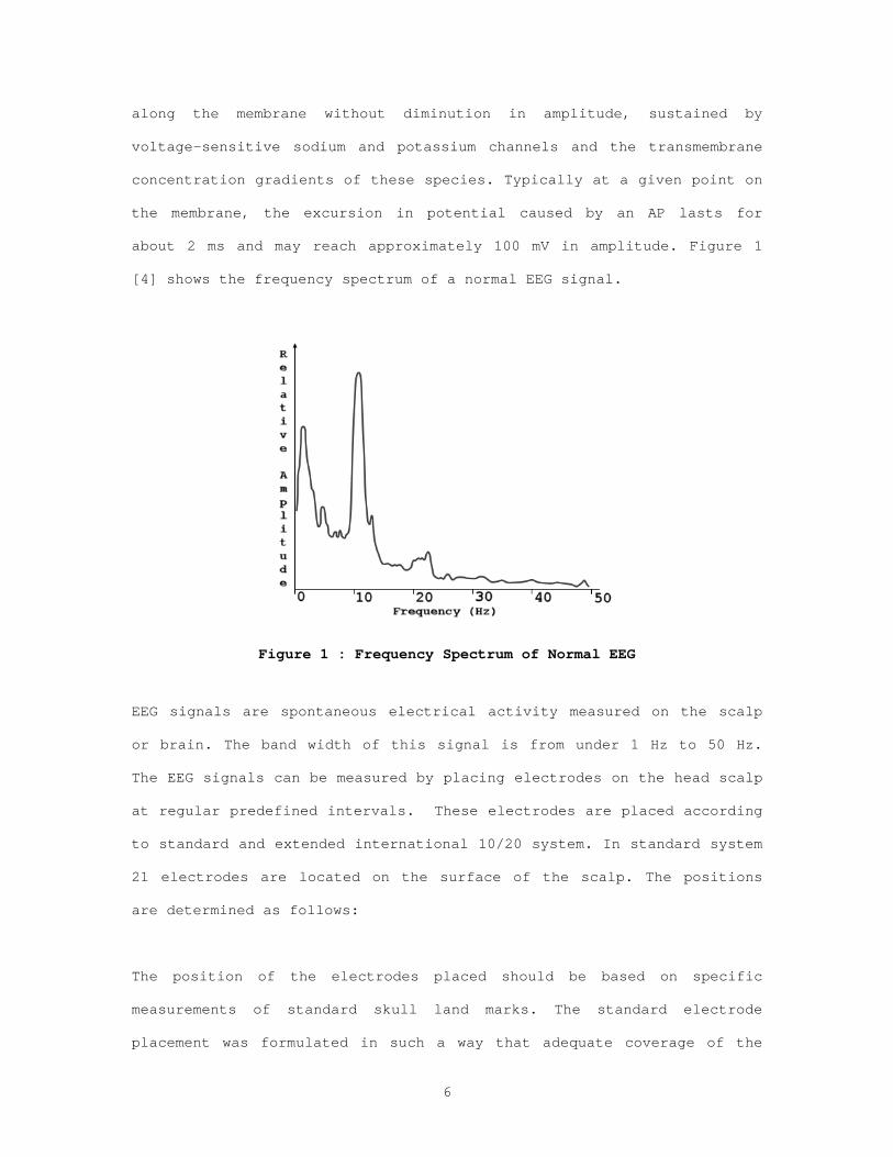
about 2 ms and may reach approximately 100 mV in amplitude. Figure 1

[4] shows the frequency spectrum of a normal EEG signal.

Figure 1 : Frequency Spectrum of Normal EEG

EEG signals are spontaneous electrical activity measured on the scalp

or brain. The band width of this signal is from under 1 Hz to 50 Hz.

The EEG signals can be measured by placing electrodes on the head scalp

at regular predefined intervals. These electrodes are placed according

to standard and extended international 10/20 system. In standard system

21 electrodes are located on the surface of the scalp. The positions

are determined as follows:

The position of the electrodes placed should be based on specific

measurements of standard skull land marks. The standard electrode

placement was formulated in such a way that adequate coverage of the

7

scalp was possible. The electrode naming/designation are done

according to its position or the brain areas the electrode covers. The

three important reference points used in 10/20 system are

- nasion, which is the delve at the top of the nose, level with the

eyes

- inion, which is the bony lump at the base of the skull on the

midline at the back of the head

- Preauricular points, which is located near the ears [13].

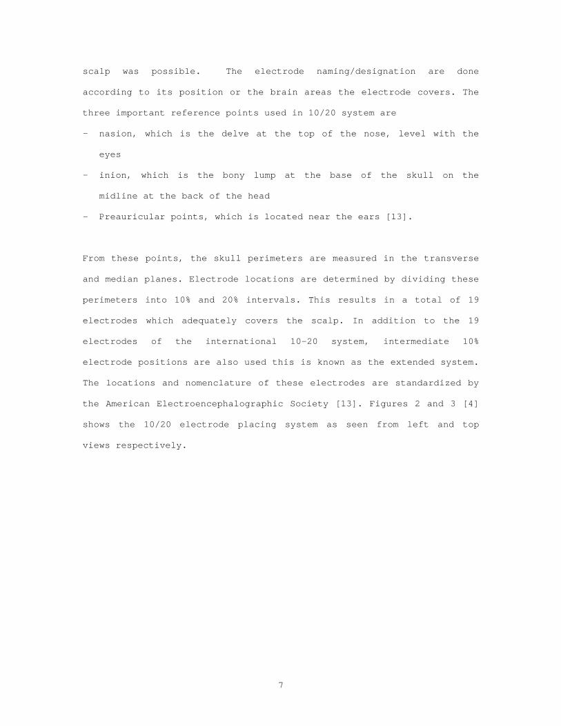
From these points, the skull perimeters are measured in the transverse

and median planes. Electrode locations are determined by dividing these

perimeters into 10% and 20% intervals. This results in a total of 19

electrodes which adequately covers the scalp. In addition to the 19

electrodes of the international 10-20 system, intermediate 10%

electrode positions are also used this is known as the extended system.

The locations and nomenclature of these electrodes are standardized by

the American Electroencephalographic Society [13]. Figures 2 and 3 [4]

shows the 10/20 electrode placing system as seen from left and top

views respectively.

8

Figure 2 : The international 10/20 system seen from left

Figure 3

: The international 10/20 system seen from top

2.1. Types of Artifacts

Before the raw data can be given as input for further processing, it

has to be preprocessed to correct it for EOGs and EMGs. Also noise from

power line has to be eliminated. Artifacts are unwanted signals

recorded during the data acquisition process. Artifacts affect the

quality of the signal hence it makes it difficult for visualization.

Artifacts can lead to wrong interpretation of data and it can change

the basic characteristics of the signal. Figure 4 [10] shows various

artifacts recorded during EEG recording.

9

Figure 4 : Types of Artifacts

Some of the commonly observed artifacts in the EEG recordings are

1. Electro Ocular Gram (EOG): EEG basically reflects the activity of

the brain. While recording the data some times the subjects might

blink hence a false signal or an artifact called EOG is generated.

The eye forms an electric dipole (Cornea being positive and retina

being negative) any eye movement would produce an electric field

around the eye which would traverse into the scalp and recorded as

an artifact while acquiring the EEG [14]. The EOG is a high

amplitude signal which masks the original signal recorded at the

particular instance of blinking with in it. If uncorrected the high

amplitude data recorded in the form of EOG can very well be

misunderstood as the signal of interest and this would lead to

faulty conclusions. Though EOG on its own can be a signal of use,

it is considered an artifact when it is not needed. For example EOG

recordings can be used to determine the gaze ions, but in

10

classification purposes using EEG, EOG is hardly considered as a

relevant data. The EOG can be eliminated by placing two electrodes

on the eye lids and record the ocular signal. This ocular signal can

be subtracted with the EEG signal recorded at that particular

instance when the eye blinks. Other way to avoid EOG is to instruct

the subject not to blink their eyes during the data acquisition. EOG

can also be eliminated by designing adaptive filters [14].

2. Electromyogram (EMG): EEG signals sometimes are intermingled with

electrical activity of the muscle tissue overlaying the skull. Also

the EMG produced by the muscles in other parts of the body

propagates through the body and can also reach the skull. Muscle

artifacts are usually observed in higher frequencies and can be

easily identified due to their high values as comparing the local

back ground activity [15].

3. Electrocardiogram (ECG): ECGs represent the activity of the heart.

Though the heart functions independent of the brain, the electrical

activity produced by the heart in the form of ECGs are recorded by

the EEG electrodes. Again an EEG wave form uncorrected for ECGs and

EMGs would look distorted and would lead to faulty analysis of the

recorded signal. The ECG artifact is not always observed.

4. Power Line Noise: Power Line signal is induced due to the power line

to which the data acquisition system is connected to. The frequency

associated with this noise is 60 Hz. The noise from the power line

can be eliminated by designing a notch filter at 60 Hz which would

remove the data at 60 Hz and thus eliminating the noise from the

power line.

11

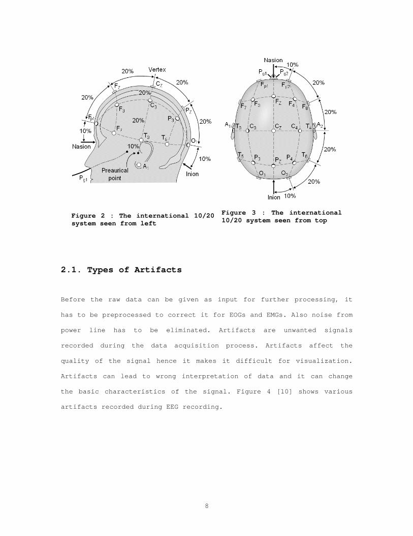
Figure 5 [11] shows the EEG power spectrum corrected for the artifacts

discussed above.

Figure 5 : Original and Reconstructed EEG Power Spectrum

2.2. Classification of EEG Signals

The EEG signals can be classified as the following

1. Evoked Potentials: Evoked potentials are signals generated due to an

external stimulus or internal stimulus [3].

2. Spontaneous Potentials: Spontaneous potentials does not depend any

external stimulus to be recorded. A good example of this would be

the EEG rhythms over sensor motor cortex [3].

3. Slow Cortical Potentials (SCP): The lowest frequency features of the

scalp recorded EEG are slow voltage changes generated in cortex.

These potentials shifts occur over 0.5-10 seconds. Negative SCP is

12

associated with movements and other functions involving cortical

activation. Positive SCP is associated with reduced with cortical

activation. People can learn to control SCPs. This can be applied to

move cursors on the computer screens [3].

4. P300 Evoked Potentials: Significant auditory, visual or

somatosensory stimuli, when interspersed with frequent or routine

stimuli it evoke EEG over the Parietal cortex which has a positive

peak at about 300 ms hence the name P300 evoked potential. Evoked

potentials are different from P300 evoked potentials as evoked

potentials do not require frequent stimuli [3].

2.3. Classification of EEG Rhythms

1. Alpha Rhythms: When people are awake, primary sensory or motor

cortical areas often display 8-13 Hz EEG activity when they are

engaged in processing sensory input or producing motor output. This

idling activity is called Alpha rhythm when focused over

somatosensory or motor cortex. Research shows that the Alpha rhythm

comprises of different 8-13 Hz rhythms, distinguished from each

other by location, frequency and relationship to concurrent sensory

input or motor output [3].

2. Beta Rhythms: Beta rhythms are associated with Alpha rhythms. Beta

rhythms are between 18-26 Hz and some Beta rhythms are harmonics of

Alpha rhythms [3].

13

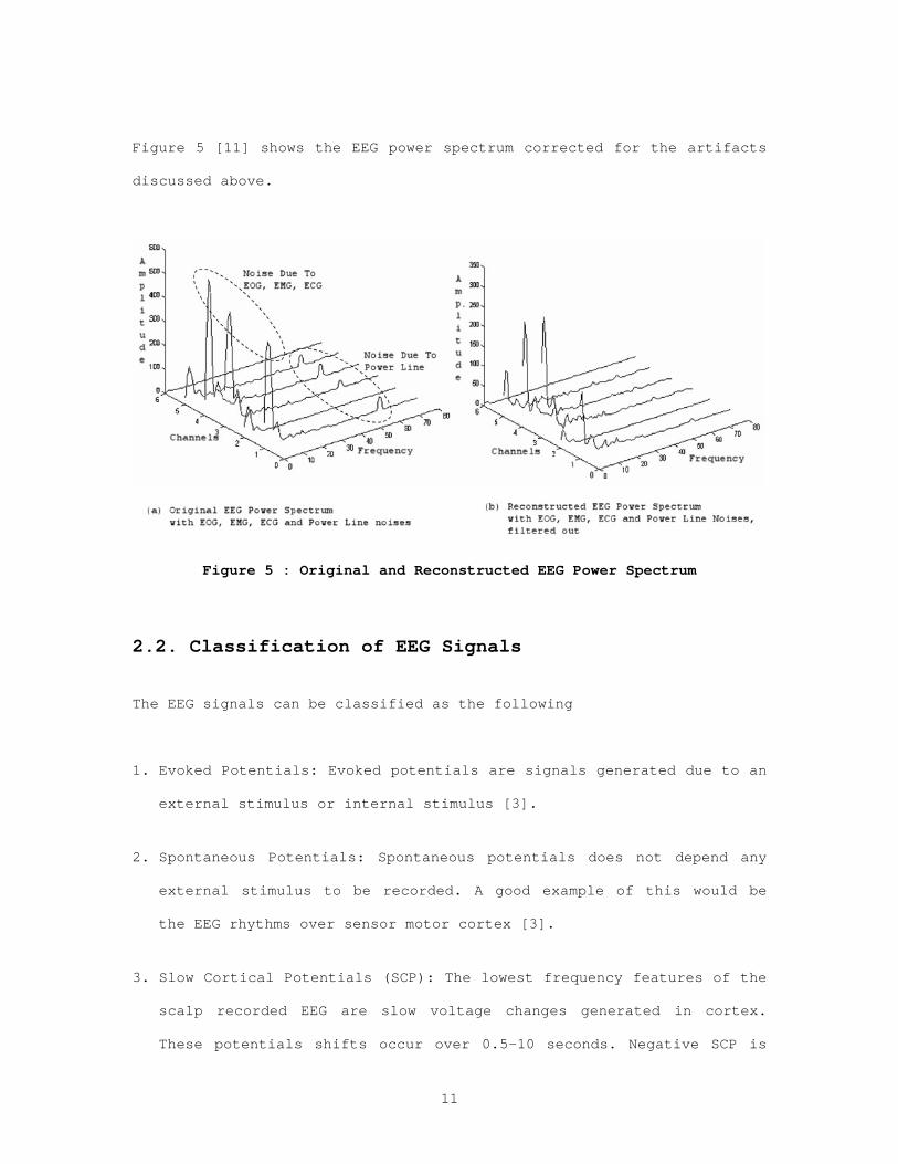
3. Delta and Theta Rhythms: Delta rhythm occupies a bandwidth of 0.5 -

4 Hz and Theta rhythms occupy a bandwidth of 4-8 Hz. These rhythms

basically reflect the EEG activity in sleeping infants and adults

respectively [3].

0 0.5 1 1.5 2 2.5 3 3.5 4 4.5 5-4-2024

Delta waves between .5 to 4 Hz

Am

plitu

de

0 0.5 1 1.5 2 2.5 3 3.5 4 4.5 5

-101

Theta waves between 4 to 8 Hz

Am

plitu

de

0 0.5 1 1.5 2 2.5 3 3.5 4 4.5 5-2

0

2

Alpha waves between 8 to 13 Hz

Am

plitu

de

0 0.5 1 1.5 2 2.5 3 3.5 4 4.5 5

-202

Beta waves between 18 to 26 Hz

Time in seconds

Am

plitu

de

Figure 6 : Example of Alpha, Beta, Theta and Delta EEG Signals

14

3. Signal Processing

Signal processing of an EEG is done to enhance and aid the recognition

of some aspect of the EEG that correlates with the physiology and

pharmacology of interest. Figure 7 shows the block diagram of a typical

EEG based task classification system.

Figure 7 : EEG based classification system Block Diagram

The signal processing consists of the following steps:

1. Filtering of raw data: The raw EEG is filtered for noise induced

from the power lines, EMG and EOG etc. Though EMG and EOG might be

useful in extracting some vital information most of the times they

hinder in proper classification. The task of filtering is

accomplished by implementing various filters like band pass filters,

low pass filters, high pass filters, and adaptive filters and by

visual inspection [8, 14].

15

2. Digitization of raw data: Digitization of raw data is performed to

convert the analog raw data into digital data. Analog signals are

continuous and smooth. Analog signals are continuous in both time

and signal. They can be measured or displayed with any degree of

precision at any moment in time. Digital signals are fundamentally

different because they represent discrete points in time and their

values are quantities to a fixed resolution rather than continuous.

The binary world of computers and digital signal processors operates

on binary numbers, which are sets of bits. Digital signals are also

quantized in time, unlike analog signals, which vary smoothly from

moment to moment. When translation from analog to digital occurs, it

occurs at specific points in time. The inverse of the separating of

the time points which is constant is called sampling frequency and

it is expressed in Hz.

3. Feature Extraction: Feature extraction involves extracting the

relevant data from the digitized data with which proper

classification can be done. Feature extraction is the most important

aspect of any classification process. The extracted feature contains

the discriminatory information hence the accuracy of feature

extraction affects the accuracy of the classification. Feature

extraction can be done in both time and frequency domain. Some

examples of time domain analysis are common spatial patters, auto

regressive parameter estimation and basic probability and

statistical analysis. Some examples of frequency domain analysis

are Fourier spectrum analysis and power spectral density estimation.

Data reduction can also be achieved in the feature extraction

process as only the relevant data is selected for classification

purposes and thus reducing the processing the time.

16

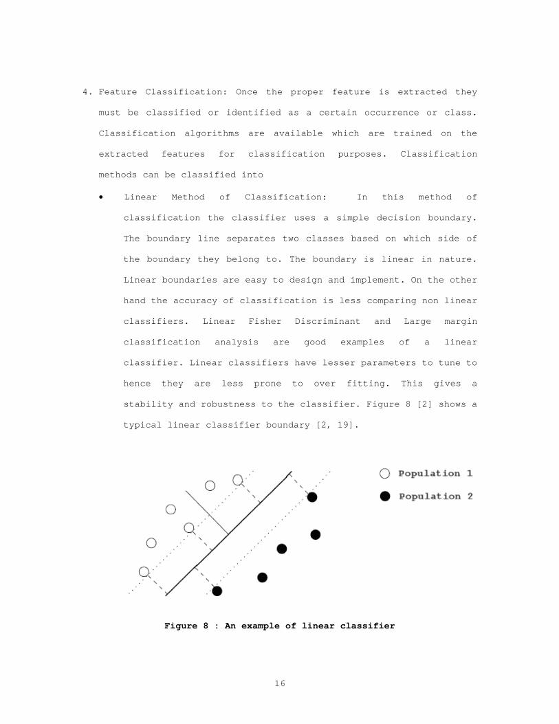
4. Feature Classification: Once the proper feature is extracted they

must be classified or identified as a certain occurrence or class.

Classification algorithms are available which are trained on the

extracted features for classification purposes. Classification

methods can be classified into

Linear Method of Classification: In this method of

classification the classifier uses a simple decision boundary.

The boundary line separates two classes based on which side of

the boundary they belong to. The boundary is linear in nature.

Linear boundaries are easy to design and implement. On the other

hand the accuracy of classification is less comparing non linear

classifiers. Linear Fisher Discriminant and Large margin

classification analysis are good examples of a linear

classifier. Linear classifiers have lesser parameters to tune to

hence they are less prone to over fitting. This gives a

stability and robustness to the classifier. Figure 8 [2] shows a

typical linear classifier boundary [2, 19].

Figure 8 : An example of linear classifier

17

Non Linear Method of Classification: In this method of

classification the classifier uses or creates boundaries based

on the nature of the classes to be separated. The boundary

surface can be irregular unlike a linear boundary. Non linear

classifiers are difficult to design and implement. The accuracy

of classification is high. Some examples of non linear

classifiers are Support Vector Machines and Artificial Neural

Networks and quadratic classifiers. The non-linear classifiers

have more parameters associated with them to tune them hence

they are prone to over fitting [2, 19]. Figure 9 [2] shows a

typical non linear classifier boundary.

Figure 9 : An example of a two dimensional non linear classifier

18

4. Optimal EEG Rhythm and Channel Pairs Selection

The process of data reduction can be divided into two stages.

Stage 1: Choosing the optimal EEG rhythm by the method of comparing

the data separability of each channel pair in each rhythm. Data

separability is defined as the extent to which a linear classifier can

correctly classify the features as features from high work load data or

low work load data. This method is called the direct method.

Stage 2: Selection of optimal EEG channels, from the data extracted

from the optimal EEG rhythm. The optimal EEG channels are chosen by

implementing the method of Common Spatial Patterns (CSP). The selection

of the optimal EEG channels is an automatic method.

The data reduction can be summarized in the following steps:

Raw data was normalized to have equal variance in all channels.

Data belonging to each rhythm was extracted for each type of task.

Data separability was tested in each rhythm for each channel pairs

respectively by using a linear classifier.

The rhythm that showed the best data separability was considered the

optimal rhythm.

The rank of the channel separability is obtained

The Common Spatial Patterns (CSP) method was applied to the data

extracted from the optimal EEG rhythm selected.

Optimal EEG channel pairs are selected based on the results of the

CSP method.

The results of the CSP method are compared with the results of the

direct method.

19

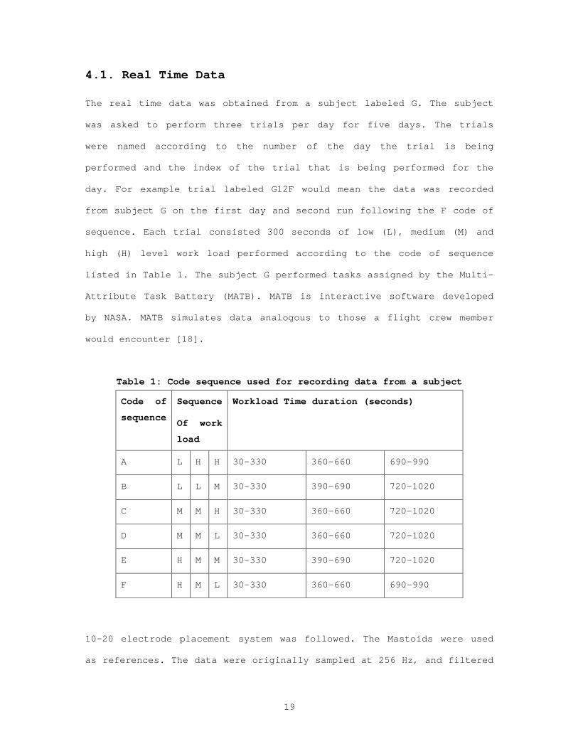
4.1. Real Time Data

The real time data was obtained from a subject labeled G. The subject

was asked to perform three trials per day for five days. The trials

were named according to the number of the day the trial is being

performed and the index of the trial that is being performed for the

day. For example trial labeled G12F would mean the data was recorded

from subject G on the first day and second run following the F code of

sequence. Each trial consisted 300 seconds of low (L), medium (M) and

high (H) level work load performed according to the code of sequence

listed in Table 1. The subject G performed tasks assigned by the Multi-

Attribute Task Battery (MATB). MATB is interactive software developed

by NASA. MATB simulates data analogous to those a flight crew member

would encounter [18].

Table 1: Code sequence used for recording data from a subject

Code of

sequence

Sequence

Of work

load

Workload Time duration (seconds)

A L H H 30-330 360-660 690-990

B L L M 30-330 390-690 720-1020

C M M H 30-330 360-660 720-1020

D M M L 30-330 360-660 720-1020

E H M M 30-330 390-690 720-1020

F H M L 30-330 360-660 690-990

10-20 electrode placement system was followed. The Mastoids were used

as references. The data were originally sampled at 256 Hz, and filtered

20

from 0.05 – 100 Hz. Data were then down sampled at 128 Hz and then

stored in .mat files. The EOG artifacts in the original data were

already corrected using MANSCAN software [20].

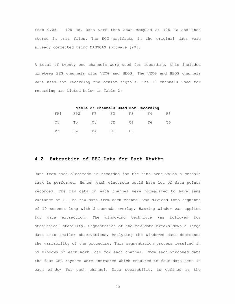
A total of twenty one channels were used for recording, this included

nineteen EEG channels plus VEOG and HEOG. The VEOG and HEOG channels

were used for recording the ocular signals. The 19 channels used for

recording are listed below in Table 2:

Table 2: Channels Used For Recording

FP1 FP2 F7 F3 FZ F4 F8

T3 T5 C3 CZ C4 T4 T6

P3 PZ P4 O1 O2

4.2. Extraction of EEG Data for Each Rhythm

Data from each electrode is recorded for the time over which a certain

task is performed. Hence, each electrode would have lot of data points

recorded. The raw data in each channel were normalized to have same

variance of 1. The raw data from each channel was divided into segments

of 10 seconds long with 5 seconds overlap. Hamming window was applied

for data extraction. The windowing technique was followed for

statistical stability. Segmentation of the raw data breaks down a large

data into smaller observations. Analyzing the windowed data decreases

the variability of the procedure. This segmentation process resulted in

59 windows of each work load for each channel. From each windowed data

the four EEG rhythms were extracted which resulted in four data sets in

each window for each channel. Data separability is defined as the

21

percentage of the correctly classified feature samples in the low and

high work load by a classifier. The data separability was tested for

each individual channel pairs in each rhythm. For example, the data

obtained from the alpha rhythm of the channel FP2 of the low level work

data was compared with data obtained from the alpha rhythm from the

channel FP2 of the high level work data.

The data from each rhythm was extracted by implementing by bandpass

filtering. The Four rhythms were extracted were the Delta rhythm (.5-4

Hz), Theta rhythm (4-8 Hz), Alpha rhythm (8-13 Hz) and Beta rhythm (13-

26 Hz).

The band pass filtering was implemented by using the following MATLAB

command

[A, B] = ellip (N, Rp, Rs, Wp)

Elliptic filters offer steeper roll off characteristics. N is the order

of the filter, Rp is the peak-to-peak ripple in decibels and Rs is the

minimum stop band attenuation in decibels. Wp is the normalized

frequency of that particular band. The normalization is done with

respect to half the sampling frequency. A and B are the filter

coefficients. The filter coefficients were applied on the EEG data and

the data from each rhythm. The filtering process was performed using

the following MATLAB command.

Y = FILTER (B, A, X)

22

Where Y is the filtered data. B and A are the filter coefficients

calculated and X is the data to be filtered.

4.3. Linear Classifier Design

Feature extraction is a process by which relevant information from the

raw data is extracted for further classification purposes. The relevant

information extracted need not be in the form of raw data. The feature

that was considered for the data separability procedure was Variance of

the signals. The feature was calculated for all windows of rhythm from

each channel for each work load data type. This resulted in 59*4*1

feature samples for each channel for each work load data. The feature

extracted this way was given as an input to a Fisher’s Linear

Classifier for analyzing the data separability.

The following equations discuss the design of Fisher’s linear

classifier [19].

Assign X0 to class 1 if Y0=M Assign X0 to class 2 if Y0<M

Y0 = (X1m - X2m)t * (Spooled)

-1 * X0

M = ½ * (X1m-X2m)t * (Spooled)

-1 * (X1m + X2m)

Spooled = [(n1-1)/((n1-1)+(n2-1))] * S1+[(n2-1)/((n1-1)+(n2-1))] * S2

Where,

Y0 is the distance of the data to be classified from the

classifier boundary M

X0 is the data to be classified

X1m and X2m are the means of the data 1 and data 2 respectively.

23

S1 and S2 are the co variance matrices of data1 and data2

respectively. The covariance here is the estimate of how much

each feature samples vary when comparing the other feature

samples in the same data set.

Spooled is the joint covariance of both the data.

n1 and n2 are number of samples in data1 and data2 respectively.

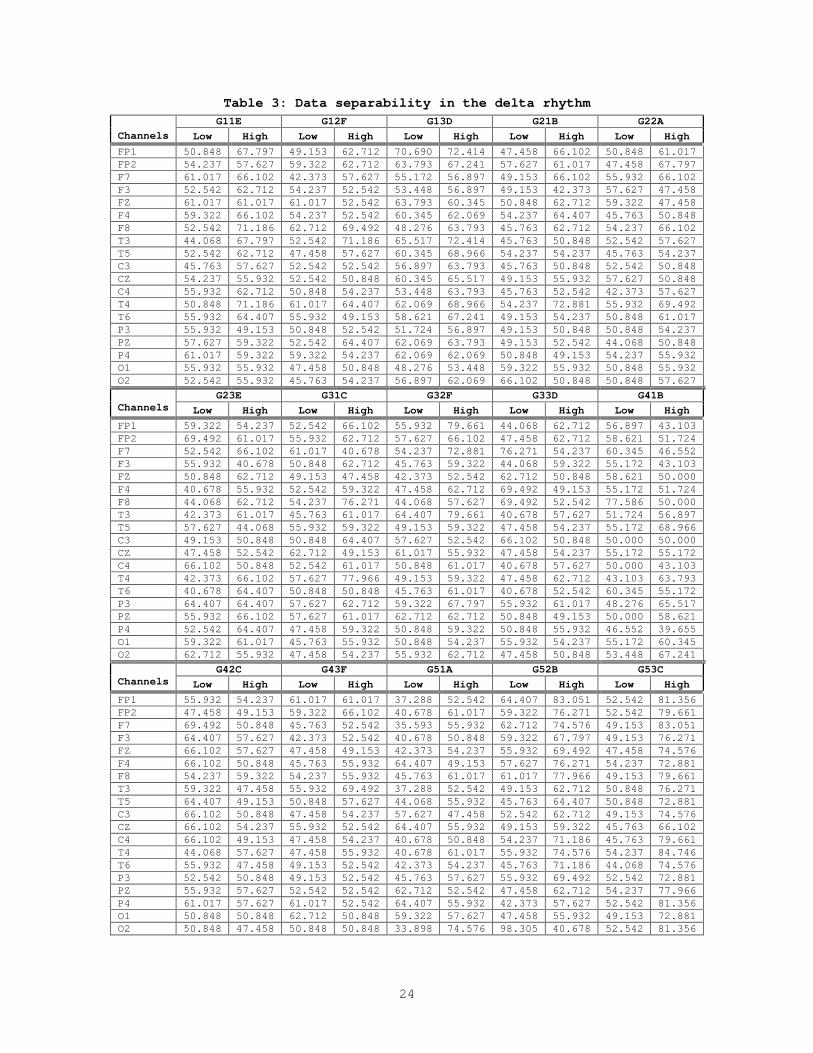
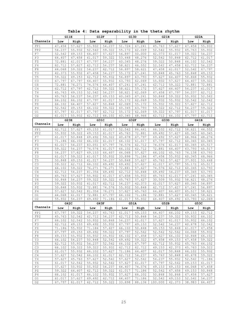
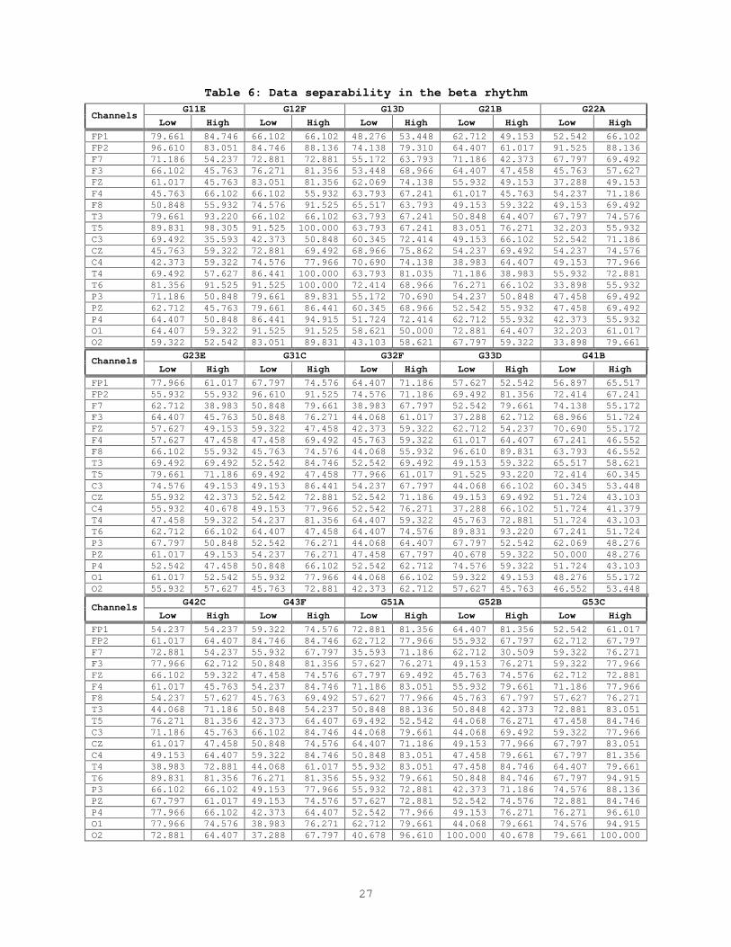
4.4. Results of Data Separability in Each Rhythm

The programming for Data separability was done in MATLAB. This method

is the method for selecting the optimal EEG rhythm. This method is

called the direct method because the linear classifier is used to

select the top 5 optimal channels based on the channel’s data

separability using variance as the feature. Then to compute the

percentage of misclassification by the optimal channels selected again

a linear classifier is implemented which computes the misclassification

percentage by using variance as the feature. The CSP method is called

the in or automatic method because the CSP method picks up the optimal

channels first and then the average misclassification percentage is

computed for the optimal channels using a linear classifier with

variance as the feature. The following tables summarize the results of

the data separability in each rhythm for all trials in the direct

method. Tables 3, 4, 5 and 6 show the separability of the two work load

data for all channels in delta, theta, alpha and beta rhythms using

variance as the feature. The entries in tables are the percentage of

correctly classified features for both work loads.

24

Table 3: Data separability in the delta rhythm

G11E G12F G13D G21B G22A

Channels Low High Low High Low High Low High Low High

FP1 50.848 67.797 49.153 62.712 70.690 72.414 47.458 66.102 50.848 61.017 FP2 54.237 57.627 59.322 62.712 63.793 67.241 57.627 61.017 47.458 67.797 F7 61.017 66.102 42.373 57.627 55.172 56.897 49.153 66.102 55.932 66.102 F3 52.542 62.712 54.237 52.542 53.448 56.897 49.153 42.373 57.627 47.458 FZ 61.017 61.017 61.017 52.542 63.793 60.345 50.848 62.712 59.322 47.458 F4 59.322 66.102 54.237 52.542 60.345 62.069 54.237 64.407 45.763 50.848 F8 52.542 71.186 62.712 69.492 48.276 63.793 45.763 62.712 54.237 66.102 T3 44.068 67.797 52.542 71.186 65.517 72.414 45.763 50.848 52.542 57.627 T5 52.542 62.712 47.458 57.627 60.345 68.966 54.237 54.237 45.763 54.237 C3 45.763 57.627 52.542 52.542 56.897 63.793 45.763 50.848 52.542 50.848 CZ 54.237 55.932 52.542 50.848 60.345 65.517 49.153 55.932 57.627 50.848 C4 55.932 62.712 50.848 54.237 53.448 63.793 45.763 52.542 42.373 57.627 T4 50.848 71.186 61.017 64.407 62.069 68.966 54.237 72.881 55.932 69.492 T6 55.932 64.407 55.932 49.153 58.621 67.241 49.153 54.237 50.848 61.017 P3 55.932 49.153 50.848 52.542 51.724 56.897 49.153 50.848 50.848 54.237 PZ 57.627 59.322 52.542 64.407 62.069 63.793 49.153 52.542 44.068 50.848 P4 61.017 59.322 59.322 54.237 62.069 62.069 50.848 49.153 54.237 55.932 O1 55.932 55.932 47.458 50.848 48.276 53.448 59.322 55.932 50.848 55.932 O2 52.542 55.932 45.763 54.237 56.897 62.069 66.102 50.848 50.848 57.627

G23E G31C G32F G33D G41B Channels Low High Low High Low High Low High Low High


G42C G43F G51A G52B G53C Channels Low High Low High Low High Low High Low High


25

Table 4: Data separability in the theta rhythm

G11E G12F G13D G21B G22A

Channels Low High Low High Low High Low High Low High


G23E G31C G32F G33D G41B Channels Low High Low High Low High Low High Low High


G42C G43F G51A G52B G53C Channels Low High Low High Low High Low High Low High


26

Table 5: Data separability in the alpha rhythm

G11E G12F G13D G21B G22A Channels

Low High Low High Low High Low High Low High


G23E G31C G32F G33D G41B Channels



G42C G43F G51A G52B G53C Channels



27

Table 6: Data separability in the beta rhythm

G11E G12F G13D G21B G22A Channels



G23E G31C G32F G33D G41B Channels



G42C G43F G51A G52B G53C Channels



28

4.5. Interpretation of the Results

Channels that showed at least 75% or higher of data separability for

each work load was considered as optimal channels. For example in beta

rhythm for subject G11E channel FP2 shows 96.61% and 83.05% of data

separability in low and high work load respectively. Since both the

percentage values were greater than 75%, they were considered as an

optimal channel pair. Likewise in theta rhythm for subject G11E channel

FP2 shows 54.23% and 55.93% of data separability in low and high work

load respectively. Since both the percentage values were lesser than

75%, they were not considered as an optimal channel pair. In beta

rhythm for subject G21B in the channel T6 for low work load data

separability of 77.9% is observed while for high work load 67.7% of

data separability is observed, channel T6 was not considered an optimal

pair as both the work loads must display data separability of at least

75% and higher.

The 75% criterion was a research specific criterion and it was not

derived from any other research information or procedures. It was

observed that there was at least one channel in the beta rhythm which

could be selected as an optimal channel for more trials when compared

to the other rhythms, hence it was concluded that only beta rhythm is

optimal rhythm for classification purposes. Figures 10 and 11 shows

example of feature samples plot of good and bad separable data obtained

from trial G11E in beta rhythm for channels FP2 and O2. The Feature

considered for the plots is the variance.

29

Figure 10 : Plot for good separable data

Figure 11 : Plot for poor separable data

30

Only certain channels showed good data separability in the Beta band.

Top 5 channels were chosen from each trial based on its data

separability percentage. This resulted in 5 optimal channels for each

trial. A generic set of 5 channels were chosen based on the number of

times a particular channel occurs in the top 5 positions considering

all 15 trials. For example FP2 appeared in 11 trials out of the 15

trials as one among the top 5 channels. It must be noted that not all

the channels chosen would meet the 75% criterion. Some channels might

show data separability of lesser than 75% but they are chosen as they

happen to be one of the top 5 highest data separability values. The top

5 channels chosen based on the data separability by the direct method

are FP2, T6, FP1, T5 and T3.

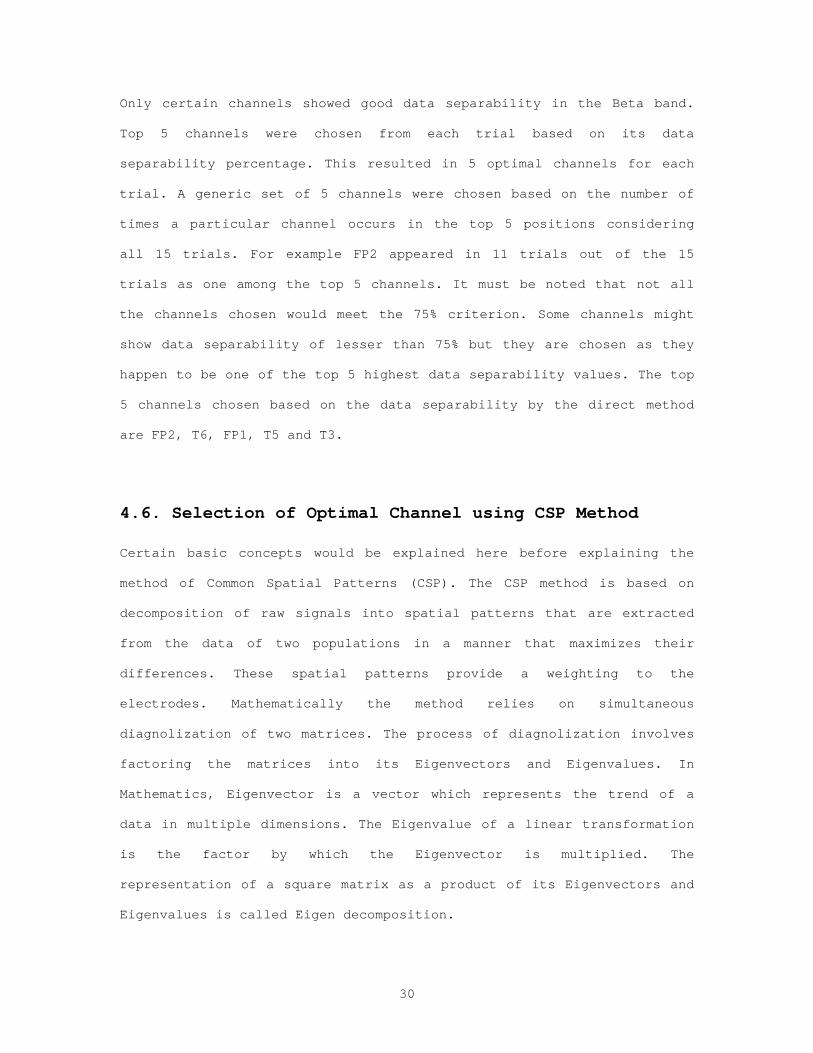
4.6. Selection of Optimal Channel using CSP Method

Certain basic concepts would be explained here before explaining the

method of Common Spatial Patterns (CSP). The CSP method is based on

decomposition of raw signals into spatial patterns that are extracted

from the data of two populations in a manner that maximizes their

differences. These spatial patterns provide a weighting to the

electrodes. Mathematically the method relies on simultaneous

diagnolization of two matrices. The process of diagnolization involves

factoring the matrices into its Eigenvectors and Eigenvalues. In

Mathematics, Eigenvector is a vector which represents the trend of a

data in multiple dimensions. The Eigenvalue of a linear transformation

is the factor by which the Eigenvector is multiplied. The

representation of a square matrix as a product of its Eigenvectors and

Eigenvalues is called Eigen decomposition.

31

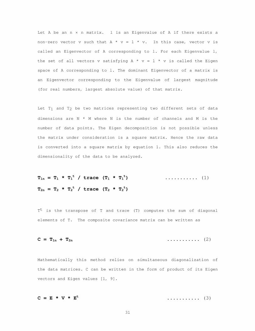
Let A be an n × n matrix. l is an Eigenvalue of A if there exists a

non-zero vector v such that A * v = l * v. In this case, vector v is

called an Eigenvector of A corresponding to l. For each Eigenvalue l,

the set of all vectors v satisfying A * v = l * v is called the Eigen

space of A corresponding to l. The dominant Eigenvector of a matrix is

an Eigenvector corresponding to the Eigenvalue of largest magnitude

(for real numbers, largest absolute value) of that matrix.

Let T1 and T2 be two matrices representing two different sets of data

dimensions are N * M where N is the number of channels and M is the

number of data points. The Eigen decomposition is not possible unless

the matrix under consideration is a square matrix. Hence the raw data

is converted into a square matrix by equation 1. This also reduces the

dimensionality of the data to be analyzed.

T1n = T1 * T1t / trace (T1 * T1

t) ........... (1)

T2n = T2 * T2t / trace (T2 * T2

t)

Tt is the transpose of T and trace (T) computes the sum of diagonal

elements of T. The composite covariance matrix can be written as

C = T1n + T2n ........... (2)

Mathematically this method relies on simultaneous diagonalization of

the data matrices. C can be written in the form of product of its Eigen

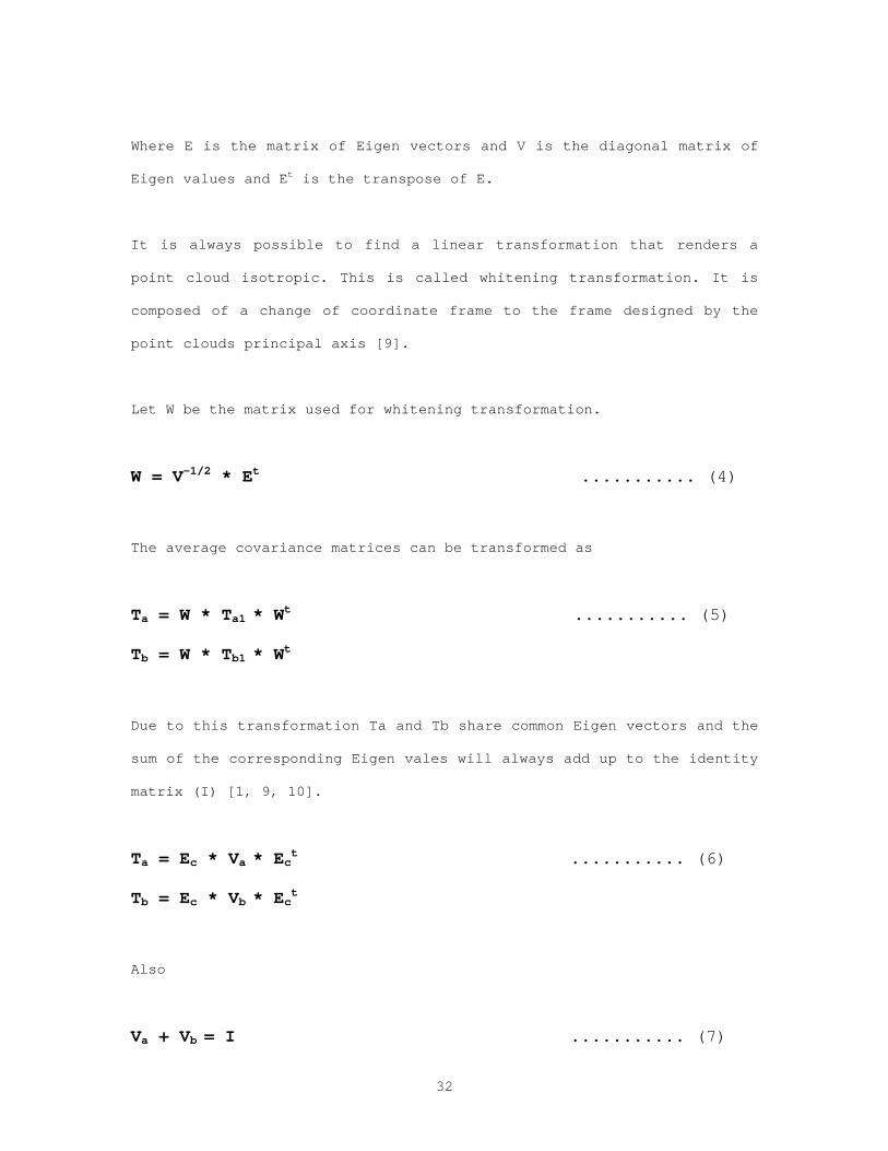
vectors and Eigen values [1, 9].

C = E * V * Et ........... (3)

32

Where E is the matrix of Eigen vectors and V is the diagonal matrix of

Eigen values and Et is the transpose of E.

It is always possible to find a linear transformation that renders a

point cloud isotropic. This is called whitening transformation. It is

composed of a change of coordinate frame to the frame designed by the

point clouds principal axis [9].

Let W be the matrix used for whitening transformation.

W = V-1/2 * Et ........... (4)

The average covariance matrices can be transformed as

Ta = W * Ta1 * Wt ........... (5)

Tb = W * Tb1 * Wt

Due to this transformation Ta and Tb share common Eigen vectors and the

sum of the corresponding Eigen vales will always add up to the identity

matrix (I) [1, 9, 10].

Ta = Ec * Va * Ect ........... (6)

Tb = Ec * Vb * Ect

Also

Va + Vb = I ........... (7)

33

The projection matrix is defined as

P = Ect * W ........... (8)

The original EEG can be transformed into uncorrelated components as

Eu = P * X ........... (9)

The original data X can be obtained by

X = P-1 * Eu ........... (10)

The columns of P-1 are spatial patterns which can be considered as EEG

source distribution vectors. The spatial patterns are arranged in the

descending order of the variances from left to right. The spatial

patterns matrix (P-1) is very similar to the matrix obtained had

principal component analysis been done on the data. The Eigenvalues of

the spatial patterns matrix are arranged from the highest to the

lowest. The Eigenvector associated with the highest Eigenvalue explains

for the majority of the variance in the combined data and this is

called the first significant Eigen vector. Channel with the highest

weight in the first significant Eigenvector is the most significant

channel and the highest weight value in the second significant

Eigenvector corresponding to the second highest Eigenvalue is the

second most significant channel and so on. The weight values for each

channel can be found out from the spatial patterns matrix [1, 9, 10].

34

4.7. Validation of the CSP Method with Simulated EEG

In section 4.7 the CSP method was demonstrated by using simple data. In

this section the CSP method would be validated by testing it on

simulated EEG signals. The simulated EEG signals can be controlled to

display variability. The EEG data was simulated by two methods which

are discussed below

Method 1: Modeling of EEG with Auto Regressive (AR) parameters:

The objective of this method is to control the variance of the input

signal and see if the CSP method is able to pick up the variance

changes. The raw data from trial G11E was used to estimate 19 AR models

of order length 8. The 19 AR models were averaged and one generic AR

model of order 8 was used for simulation of EEG data from the white

noise. The AR parameters were obtained using Burg’s method [17]. White

noise signals were used to create two data sets with 7 channels and

with 500 points in each channel. Suppose if two data sets were created

as X1 and X2, the white noise signals were initially similar in all

channels in both the data sets. Channels 1, 3 and 7 in X1 were

multiplied by constants 1.41, 2 and 2.82. By multiplying these

constants the variance of the signals in 1, 3 and 7 are varied two

times, four times and eight times than its counterparts in X2.

The generic AR parameters were applied on the X1 and X2 data for each

channel individually. The resulting output is the simulated EEG signal

labeled X1s and X2s.

35

CSP algorithm was used to detect the optimal channels. The expected

ranking is channel pair 1, 3 and 7 as the top 3 channel pairs, channel

pair 1 being the most significant channel. The CSP method was able to

pick up the significant channels in the expected order. Table 7 shows

the spatial patterns matrix and the variance ratios calculated for each

channel pairs.

Table 7: Results of Simulation with auto regressive parameters

0.0045

0.0101

0.5292

0.0066

0.0125

0.0060

0.0075

0.0056

0.0087

0.0101

0.0219

0.0477

0.2894

0.3350

0.0099

0.5744

0.0145

0.0043

0.0154

0.0004

0.0122

0.0034

0.0119

0.0030

0.2300

0.1059

0.2684

0.1925

0.0191

0.0110

0.0073

0.2014

0.3265

0.1615

0.1883

0.0127

0.0031

0.0042

0.3319

0.2834

0.1023

0.0912

Spatial Patterns

Matrix

0.7720

0.0069

0.0138

0.0116

0.0369

0.0035

0.0124

var(X1s') 2.2198

1.0133

3.6475

0.8953

1.0712

1.0857

8.1629

var(X2s') 1.1166

1.0132

0.9193

0.8817

1.0628

1.0615

1.0475

Var(X1s')/var(X2s')

1.9881

1.0001

3.9676

1.0155

1.0080

1.0228

7.7931

The CSP algorithm picks channel pair 7 as the significant channel

followed by channel pairs 3 and 1. When the variance ratios were

calculated for each channel pair and arranged in the descending order

they followed the same pattern. This simulation was repeated for 10

times with different white noise generated and the CSP method

accurately picked up the optimal channels. The variance in channels 1,3

36

and 7 of data set 1 were also changed to 3, 9 and 12 and the CSP method

picked the optimal channels according to the variance differences.

Method 2: IIR Filter Design for EEG Simulation:

In method 2, similar to method 1 two sets of data were generated using

the white noise. The Magnitude response for each channel was calculated

using the complete data from trial G11E. The IIR filter parameters were

calculated for a specified order of 8 using the MATLAB command

yulewalk. IIR filters have infinite impulse response function which is

non zero over an infinite length of time [17]. This resulted in 19

sets of IIR filter parameters which were averaged to form a generic IIR

filter parameters.

[b , a] = yulewalk (order, frequency, magnitude)

The above MATLAB command calculates the IIR parameters b and a of

specified order for a given magnitude response. The generic parameters

are found out by averaging the 19 values of b (an array of size defined

by the order) and a (an array of size defined by the order). It was

labeled as A and B. The designed filter was applied on the white noise

data and hence EEG signals were simulated which were similar in nature

in both X1 and X2.

Three amplitude responses were designed and applied to channels 1, 3

and 7 of X2 to change their power spectrum. The following figures show

the amplitude responses that were applied to channels 1, 3 and 7 in X2

respectively. The variance of the signals were made to 1 by scaling

37

the simulated signals values with a constant calculated as square root

(1/[Variance of the signal]). Thus the only varying parameter in this

case was the shape of the spectrum. The variance values of all the

channels were verified and they turned out to be 1. The designed

amplitude responses were applied on the simulated EEG signals by the

following MATLAB commands.

Y = filter (B, A, data)

The b and a coefficients calculated above in the yulewalk command is

used to filter the simulated EEG signal to vary its amplitude spectrum.

The following plots show the various amplitude responses designed and

plots of spectrums obtained after the IIR coefficients were applied on

the simulated EEG signal to change it amplitude response shape. The

motive behind this experiment is to see if the CSP method would respond

to changes in the shape of the power spectrum while the same variance

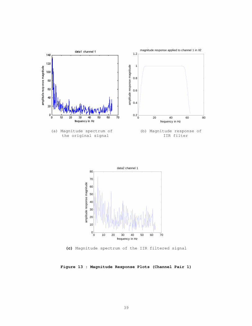
is maintained. Figure 13 shows the plots for channel pair 2. The

magnitude response of the channel pair 2 data is the original unaltered

response in all channel pairs. Figures 14, 15 and 16 shows plots of the

magnitude responses before and after applying the designed IIR filter

on channels 1, 3 and 7 in data set X2.

38

0 20 40 60 800

20

40

60

80

100

120

140

frequency in Hz

ampl

itude

res

pons

e m

agni

tude

data1 channel 2

0 20 40 60 800

20

40

60

80

100

120

140

frequency in Hz

ampl

itude

res

pons

e m

agni

tude

data2 channel 2

(a) Magnitude spectrum of (b) Magnitude spectrum of the simulated signal the IIR filtered signal

Figure 12 : Magnitude Response Plots (Channel Pair 2)

39

0 20 40 60 800.2

0.4

0.6

0.8

1

1.2

frequency in Hz

ampl

itude

res

pons

e m

agni

tude

magnitude response applied to channel 1 in X2

(a) Magnitude spectrum of (b) Magnitude response of the original signal IIR filter

0 10 20 30 40 50 60 700

10

20

30

40

50

60

70

80

frequency in Hz

ampl

itude

res

pons

e m

agni

tude

data2 channel 1

(c) Magnitude spectrum of the IIR filtered signal


40

0 10 20 30 40 50 60 700

20

40

60

80

100

120

140

160

180

frequency in Hz

ampl

itude

res

pons

e m

agni

tude

data1 channel 3

0 20 40 60 800.1

0.2

0.3

0.4

0.5

0.6

0.7

0.8

0.9

1

frequency in Hz

ampl

itude

res

pons

e m

agni

tude



0 10 20 30 40 50 60 700

10

20

30

40

50

60

70

frequency in Hz

ampl

itude

res

pons

e m

agni

tude

data2 channel 3



41

0 10 20 30 40 50 60 700

20

40

60

80

100

120

frequency in Hz

ampl

itude

res

pons

e m

agni

tude

data1 channel 7

0 20 40 60 800

0.1

0.2

0.3

0.4

0.5

frequency in Hz

ampl

itude

resp

onse

mag

nitu

de



0 10 20 30 40 50 60 700

10

20

30

40

50

60

70

80

frequency in Hz

ampl

itude

res

pons

e m

agni

tude

data2 channel 7



42

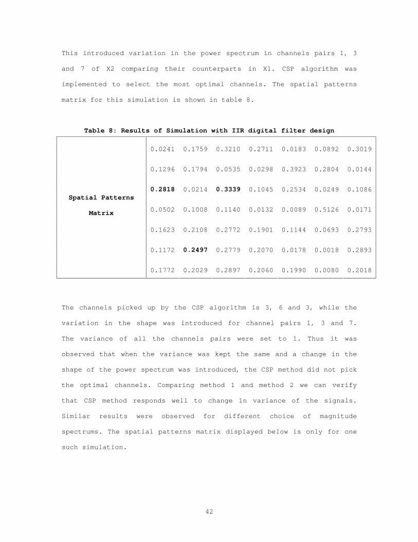
This introduced variation in the power spectrum in channels pairs 1, 3

and 7 of X2 comparing their counterparts in X1. CSP algorithm was

implemented to select the most optimal channels. The spatial patterns

matrix for this simulation is shown in table 8.

Table 8: Results of Simulation with IIR digital filter design

0.0241

0.1759

0.3210

0.2711

0.0183

0.0892

0.3019

0.1296

0.1794

0.0535

0.0298

0.3923

0.2804

0.0144

0.2818

0.0214

0.3339

0.1045

0.2534

0.0249

0.1086

0.0502

0.1008

0.1140

0.0132

0.0089

0.5126

0.0171

0.1623

0.2108

0.2772

0.1901

0.1144

0.0693

0.2793

0.1172

0.2497

0.2779

0.2070

0.0178

0.0018

0.2893

Spatial Patterns

Matrix

0.1772

0.2029

0.2897

0.2060

0.1990

0.0080

0.2018

The channels picked up by the CSP algorithm is 3, 6 and 3, while the

variation in the shape was introduced for channel pairs 1, 3 and 7.

The variance of all the channels pairs were set to 1. Thus it was

observed that when the variance was kept the same and a change in the

shape of the power spectrum was introduced, the CSP method did not pick

the optimal channels. Comparing method 1 and method 2 we can verify

that CSP method responds well to change in variance of the signals.

Similar results were observed for different choice of magnitude

spectrums. The spatial patterns matrix displayed below is only for one

such simulation.

43

4.8. Selection of Optimal Channels using Real Time Data

Data from beta rhythm was selected and the CSP method was implemented

to choose the top 5 optimal channels from beta rhythm. A moving hamming

window of 10 seconds in length with 5 seconds overlap was used to

extract data from the beta rhythm. This resulted in 59 windows. The CSP

method was applied to data extracted from each window and 5 optimal

channels were chosen for each window which resulted in totally 295

(59*5) optimal channels for a particular trial. Five channels were

chosen based on the number of times a particular channel occurs in the

total 295 channels selected. In this way 5 channels were selected for

each trial. A final set of 5 optimal channels were selected based on

the number of times a particular channels occurs in the top 5 positions

considering all trials.

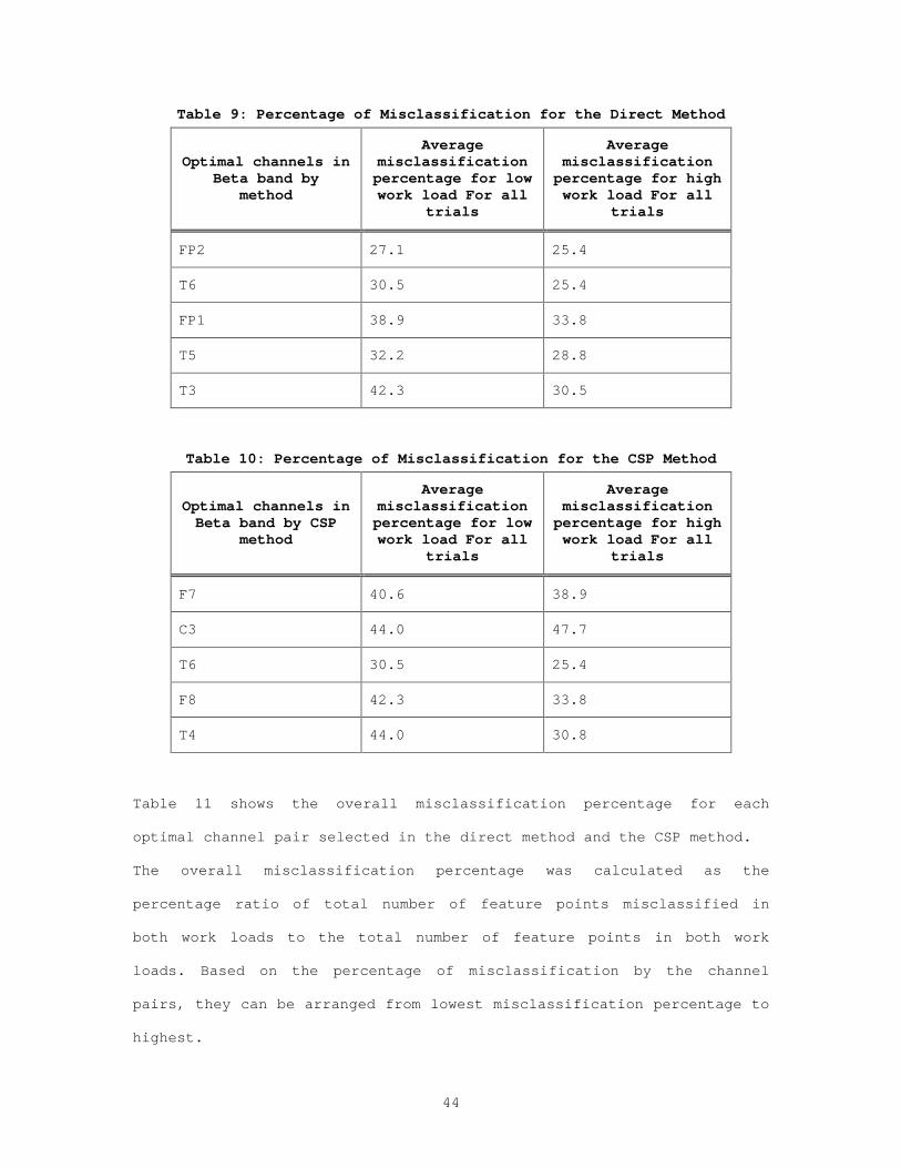
Channels F7, C3, T6, F8, and T4 were selected as the final optimal EEG

channels. Table 9 shows the average misclassification percentage of all

trials for each of the optimal channels selected by the direct method

discussed in section 4.4. The misclassification percentage was

calculated as the ratio of number of feature points misclassified to

the total number of features in that particular type of workload. The

variance of the signals in each channel was used as the feature. Table

10 shows the shows the average misclassification percentage of all

trials for each of the optimal channels selected by the CSP method.

Table 11 shows the overall percentage of misclassification for the and

the CSP method.

44

Table 9: Percentage of Misclassification for the Direct Method

Optimal channels in Beta band by

method

Average misclassification percentage for low work load For all

trials

Average misclassification percentage for high work load For all

trials

FP2 27.1 25.4

T6 30.5 25.4

FP1 38.9 33.8

T5 32.2 28.8

T3 42.3 30.5

Table 10: Percentage of Misclassification for the CSP Method

Optimal channels in Beta band by CSP

method

Average misclassification percentage for low work load For all

trials

Average misclassification percentage for high work load For all

trials

F7 40.6 38.9

C3 44.0 47.7

T6 30.5 25.4

F8 42.3 33.8

T4 44.0 30.8

Table 11 shows the overall misclassification percentage for each

optimal channel pair selected in the direct method and the CSP method.

The overall misclassification percentage was calculated as the

percentage ratio of total number of feature points misclassified in

both work loads to the total number of feature points in both work

loads. Based on the percentage of misclassification by the channel

pairs, they can be arranged from lowest misclassification percentage to

highest.

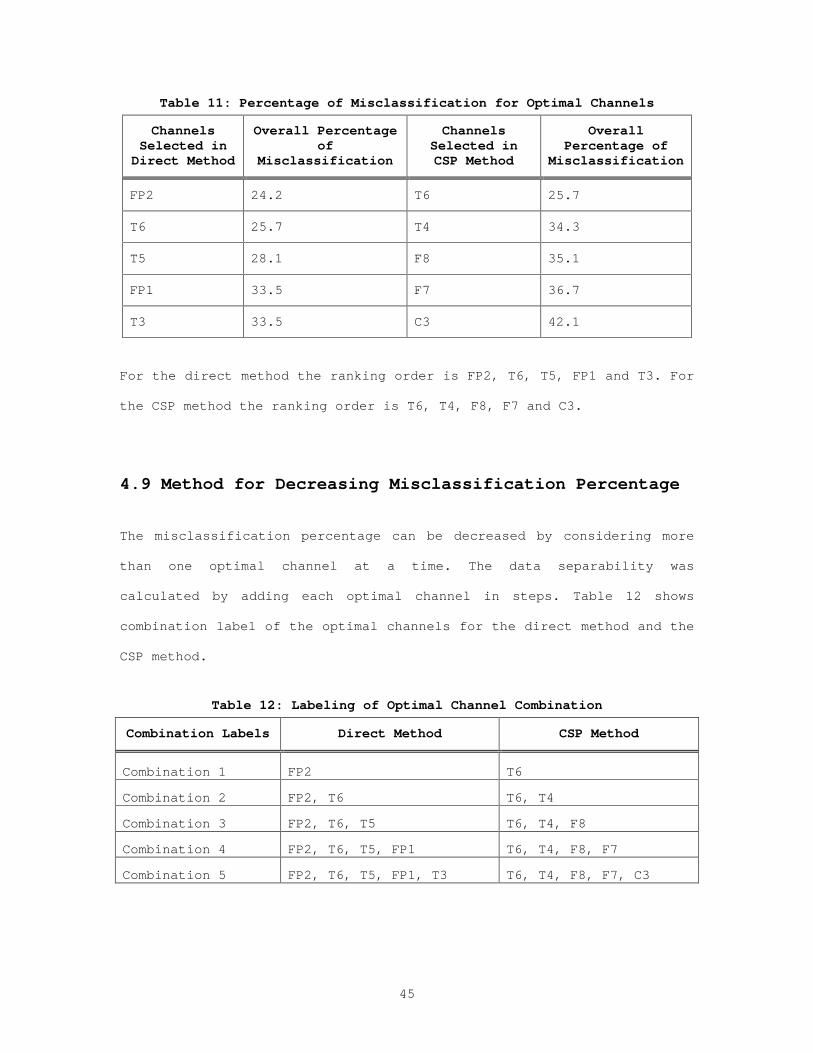
45

Table 11: Percentage of Misclassification for Optimal Channels

Channels Selected in

Direct Method

Overall Percentage of

Misclassification

Channels Selected in CSP Method

Overall Percentage of

Misclassification

FP2 24.2 T6 25.7

T6 25.7 T4 34.3

T5 28.1 F8 35.1

FP1 33.5 F7 36.7

T3 33.5 C3 42.1

For the direct method the ranking order is FP2, T6, T5, FP1 and T3. For

the CSP method the ranking order is T6, T4, F8, F7 and C3.

4.9 Method for Decreasing Misclassification Percentage

The misclassification percentage can be decreased by considering more

than one optimal channel at a time. The data separability was

calculated by adding each optimal channel in steps. Table 12 shows

combination label of the optimal channels for the direct method and the

CSP method.

Table 12: Labeling of Optimal Channel Combination

Combination Labels Direct Method CSP Method

Combination 1 FP2 T6

Combination 2 FP2, T6 T6, T4

Combination 3 FP2, T6, T5 T6, T4, F8

Combination 4 FP2, T6, T5, FP1 T6, T4, F8, F7

Combination 5 FP2, T6, T5, FP1, T3 T6, T4, F8, F7, C3

46

Table 13 shows the misclassification percentage for each channel

combination for both direct and CSP method. It can be clearly seen that

with addition of every optimal EEG channel the percentage of

misclassification dropped down. The optimal channels chosen for this

subject was T6, T4, F8, F7 and C3.

Table 13: Percentage of Misclassification for Each Combination

Combination Labels Overall Percentage of Misclassification in

Direct Method

Overall Percentage of Misclassification in

CSP Method

Combination 1 23.1 25.1





In section 4.8 it was concluded that the CSP method picks variation in

the variance. That is the CSP method should pick up the channels that

show difference in variance for low work load and high work load.

Similar to section 4.4 the differences in the variance were computed

for high work load and low work load data for all channels for all

trials in the beta rhythm. Five channels corresponding to first five

highest absolute difference values were chosen for each trial. Based on

the number of times a particular channel occurs over all trials in one

of the top 5 positions five channels were selected as a final set of

top five channels for all trials.

Channels T5, T6, F8, C3 and T4 were chosen as the five generic optimal

channels in this method. The average percentage of misclassification of

the data extracted from these channels was computed as discussed in

section 4.9. The average percentage of misclassification in this method

47

was 15.52%. The CSP method picked T6, T4, F8, F7 and C3 as the top five

generic optimal channels for this subject in the beta rhythm. It can be

observed that channels T6, F8, C3 and T4 were picked up by both the

methods. The average percentage of misclassification for this method

was 16.6%.

48

5. Discussion

The data separability was computed using variance as the feature of the

data extracted from the beta band. Variance was calculated from each 10

seconds segment to form the feature samples. But the same was not

observed in the data extracted for each rhythm. The mean variance of

the data extracted from the beta of each optimal channel of all the

windows for all trials were computed. This resulted in 75 (15*5)

variance values for each type of work load. It was found that 58 out of

the 75 variance values in the low level work load was greater than

variance values in the high level work load.

On analyzing the channel pairs selected by the CSP method it was

observed that channels F7 and F8 lie on the frontal portion of the

brain which is related to reasoning and problem solving and channels T6

and T4 lie on the temporal portion of the brain which deals with memory

[5]. The MATB assigns task which would make the subject think and

perform. Given the nature of the tasks assigned the location optimal

channels agree with the tasks being performed.

49

6. Conclusion & Future Works

An automatic method (CSP method) for choosing the Optimal EEG channels

was implemented. The method for choosing the optimal EEG rhythm was not

an automatic process (Direct method discussed in section 4.4). The

accuracy of the automatic channel selection method was tested using the

simulated data. The optimal channels selected may vary from subject to

subject. This research only dealt with choosing optimal channels for a

specific subject. Subject to subject Optimal EEG channels selection was

not investigated.

The feature that was used for the classification purpose was the

variance of the signal extracted from each window. The direct method

was only used to find the optimal EEG rhythm. Methods for

differentiating more than two tasks can also be explored. The

performance of the classification can be analyzed by experimenting with

various types of features. Different classifiers can also be used to

see if the data separability can be improved. More than one optimal EEG

rhythm could be considered to extract more information for

classification purposes. Trials recorded over 5 days were used for this

research purpose. Trials recorded for more number of days can be used

for the channel selection process as considering more days gives more

stability to the method and more clarity.

50

References 1. Yijun Wang, Shangkai Gao, Xiaorong Gao (2005), “Common Spatial

Pattern For Channel Selection In Motor Imagery Based Brain-Computer Interface”, Proceedings of the 2005 IEEE, Engineering in Medicine and Biology 27th Annual Conference.

2. Klaus-Robert Muller, Charles W. Anderson, Gary E. Birch (June 2003), “Linear And Nonlinear Methods for Brain-Computer Interfaces”, IEEE Transactions on Neural Systems and Rehabilitation Engineering, Vol. 11, NO. 2.

3. Jonathan R. Wolpaw, Niels Birbaumer, Dennis J. McFarland, Gert Pfurtscheller, Theresa M. Vaughan (2002), “Brain-Computer interfaces For Communication and Control”, Clinical Neurophysiology 113 Pg 767-791.

4. Jaakko Malmivuo, Robert Plansey (1995). “Electroencephalography. Bioelectromagnetism” (Oxford University Press, New York, USA, 1995), Chapter 13.

5. Eric H. Chudler (2007), “Lobes of the Brain”, Neuroscience for Kids.

6. Rampil, Ira J (October 1998), Primer for EEG Signal Processing in Anesthesia. Anesthesiology: Volume 89(4) pp 980-1002.

7. Ricardo Nuno Vigario (October 2001), “From Principal to Independent Component Analysis of Brain signals”, Proceedings of 23rd Annual EBMS International Conference.

8. Herbert Ramoser, Johannes Muller-Gerking and Gert Pfurtscheller (December 2000). “Optimal Spatial Filtering of single Trial EEG during Imagined Hand movement”, IEEE transactions on Rehabilitation Engineering, Vol 8, No.4.

9. Johannes Muller-Gerking, Gert Pfurtscheller, Henrik Flyvbjerg (September 1998) “Designing Optimal Spatial Filters for single Trial EEG Classification in a movement task”, Clinical Neurophysiology 110, Pg 787-798.

10. Weidong Zhou, Jin Zhou, Hao Zhao, Liu Ju (September 2005), “Removing Eye Movement and Powerline Artifacts from EEG based on ICA”, Proceedings of the 2005 IEEE, Engineering in Medicine and Biology 27th Annual Conference.

11. Terry Rybak (2005), “Is It Really Power-Line Noise Or Something Else?”, The Issue of Power-Line Noise, American Radio Relay League, Chapter 4.

12. M.Teplan (2002), “Fundementals of EEG measurement”, Measurement Science Review, Volume 2, Section 2.

51

13. H.H. Jasper (1958), “The ten-twenty electrode system of the

International Federation”, Electroencephalography and Clinical Neurophysiology, Pg 371-375.

14. P. He, M. Kahle, G. Wilson and C. Russel (September 2005), “Removal of Ocular Artifacts from EEG: A Comparison of Adaptive Filtering and Regression Method Using Simulated Data”, Proceedings of the 2005 IEEE, Engineering in Medicine and Biology 27th Annual Conference.

15. Daniel P. Brunner, Raymond C. Vasko, Christopher S. Detka, James P. Monahan, Charles F. Reynolds

and David J. Kupper (1996), “Muscle artifacts in the sleep EEG: Automated detection and effect on all-night EEG power spectra”, J. Sleep Res 5, Pg 155-164.

16. John G. Webster (1998), “MEDICAL INSTRUMENTATION Application and Design”, Third Edition, John Wiley & Sons, Inc.

17. John G. Proakis, Dimitris G. Manolakis (2007), “DIGITAL SIGNAL PROCESSING Principles, Algorithms and Applications”, Fourth Edition, Pearson Education, Inc.

18. R.O. Duda. P.E. Hart and D.G. Stork (2001), “Pattern Classification”, New York: Wiley.

19. Sams Technology Inc (2006). Manscan - state-of-the-art system for performing high-resolution EEG and event-related potential (ERP) studies. Retrieved April 11, 2007, http://www.manscaneeg.com

http://www.manscaneeg.com

52

Appendix A – Acronyms

AP Regenerative Action Potentials

BCI Brain Computer Interface

CAR Common Average Reference

CSD Current Source Derivations

CSP Common Spatial Patterns

ECG Electrocardiogram

EEG Electroencephalogram

EMG Electromyogram

EOG Electrooculogram

ERD Event Related Desynchronization

ERS Event Related Synchronization

PSP Postsynaptic Potentials

SCP Slow Cortical Potentials

MATB Multi-Attribute Task Battery

AR Auto Regression

IIR Infinite Impulse Response

NASA National Aeronautics and Space Administration

53

Appendix B – Labeling of the Electrodes

The Electrodes used were labeled based on certain conventions and the

location on the scalp. The brain can be divided into four lobes they

are

Frontal(F)

The Frontal lobe is situated in front of the central sulcus.

Sulci are the fissures observed in the brain. The Frontal lobe is

associated with reasoning, planning, problem solving and emotions

[5].

Parietal(P)

Parietal lobe is located behind central sulcus. This lobe is

associated with stimuli related to touch, pressure, temperature

and pain [5].

Temporal(T)

Temporal lobe is located below the Parietal lobe. This lobe is

associated with perception and recognition of auditory stimuli

and memory [5].

Occipital(O)

Occipital lobe is located in the back of the brain. This lobe is

associated with many aspects of vision [5].

The labeling of the electrodes is derived from the representations (F,

P, T and O) of the brain lobes. So the FP in FP2 would be Frontal-

Parietal 2.

54

Appendix C – Optimal Rhythm selection(MATLAB Code)

%This Program directmethod.m is the direct method. %The Optimal EEG rhythm is found out using this program. %The program computes data separability for each channel for each rhythm. %The program automatically accpets the data for all trials. %The output of the program is the data separability of each channel in each %trial for the selected rhythm. %The Channels used for EEG data acquisition is shown below. %FP1(1),FP2(2),F7(3),F3(4),FZ(5),F4(6),F8(7),T3(8),T5(9),C3(10),CZ(11),C4(12),T4(13),T6(14),P3(15),PZ(16),P4(17),O1(18),O2(19).

% ------------------------------------------------------------------------- clc clear all close all warning off band=input('enter the band to be analyzed as del the alp or bet with in single quotes ') for sek=1:15 %loop for accepting data from each trial seqz=['E' 'F' 'D' 'B' 'A' 'E' 'C' 'F' 'D' 'B' 'C' 'F' 'A' 'B' 'C']; seq=seqz(sek); fil=['G11Eraw'; 'G12Fraw'; 'G13Draw'; 'G21Braw'; 'G22Araw'; 'G23Eraw'; 'G31Craw'; 'G32Fraw'; 'G33Draw'; 'G41Braw'; 'G42Craw'; 'G43Fraw' ; 'G51Araw'; 'G52Braw'; 'G53Craw']; filename=fil(sek:sek,1:7);

load(filename); % Load the structure rawdata fprintf('\n') sf = 128; % sf has been lowered from the original 256 to 128 r = rawdata; clear rawdata; eegdata = [r.elec1 r.elec2 r.elec3 r.elec4 r.elec5 r.elec6 r.elec7 r.elec8 r.elec9... r.elec10 r.elec11 r.elec12 r.elec13 r.elec14 r.elec15 r.elec16 r.elec17... r.elec18 r.elec19 r.elec20 r.elec21]; datalabels = r.labels; fname1 = 'MATB-Cap19.locs'; data = eegdata(:,1:19); %EEG data A=[30 330 360 660 690 990]; B=[30 330 390 690 720 1020]; C=[30 330 360 660 720 1020]; D=[30 330 360 660 720 1017]; E=[30 330 390 690 720 1020]; F=[30 330 360 660 690 990];

numofchn=19;

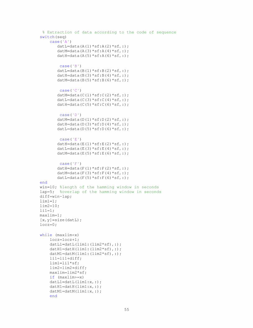
55

% Extraction of data according to the code of sequence switch(seq)

case('A') datL=data(A(1)*sf:A(2)*sf,:); datM=data(A(3)*sf:A(4)*sf,:); datH=data(A(5)*sf:A(6)*sf,:); case('B') datL=data(B(1)*sf:B(2)*sf,:); datH=data(B(3)*sf:B(4)*sf,:); datM=data(B(5)*sf:B(6)*sf,:); case('C') datM=data(C(1)*sf:C(2)*sf,:); datL=data(C(3)*sf:C(4)*sf,:); datH=data(C(5)*sf:C(6)*sf,:); case('D') datM=data(D(1)*sf:D(2)*sf,:); datH=data(D(3)*sf:D(4)*sf,:); datL=data(D(5)*sf:D(6)*sf,:); case('E') datH=data(E(1)*sf:E(2)*sf,:); datL=data(E(3)*sf:E(4)*sf,:); datM=data(E(5)*sf:E(6)*sf,:); case('F') datH=data(F(1)*sf:F(2)*sf,:); datM=data(F(3)*sf:F(4)*sf,:); datL=data(F(5)*sf:F(6)*sf,:); end

win=10; %length of the hamming window in seconds lap=5; %overlap of the hamming window in seconds diff=win-lap; lim1=1; lim2=10; li1=1;

maxlim=1; [x,y]=size(datL); locz=0;

while (maxlim<x) locz=locz+1; datL1=datL(lim1:(lim2*sf),:); datH1=datH(lim1:(lim2*sf),:); datM1=datM(lim1:(lim2*sf),:); li1=li1+diff; lim1=li1*sf; lim2=lim2+diff; maxlim=lim2*sf; if (maxlim>=x) datL1=datL(lim1:x,:); datH1=datH(lim1:x,:); datM1=datM(lim1:x,:); end

56

[x1,y1]=size(datL1); fL=zeros(1:x1,1:1); fH=zeros(1:x1,1:1); fM=zeros(1:x1,1:1); %***the four EEG rhythms

alp=[8 13]/64; bet=[18 26]/64; del=[.5 4]/64; the= [4 8]/64; %*************************

[x1,y1]=size(datL1); for hum=1:19 datL1(1:x1,hum:hum)=datL1(1:x1,hum:hum).*hamming(x1); datH1(1:x1,hum:hum)=datH1(1:x1,hum:hum).*hamming(x1); end %***Filtering og the raw data to extract data from each rhythm***

switch(band) case('alp') ban=alp;

case('bet') ban=bet; case('the') ban=the;

case('del') ban=del;

case('full') X1=datL1'; X2=datH1'; end [b,a]=ellip(4,6,50,ban); X1=filter(b,a,datL1); X2=filter(b,a,datH1); X1=X1'; X2=X2'; %****************************************************************

fet1b(locz:locz,:)=log((var(X1'))); %Feature samples for low work load fet2b(locz:locz,:)=log((var(X2'))); %Feature samples for high work load

end

%** Design of Linear classifier and Data separability computation*** for i=1:numofchn

buff1=fet1b(:,i:i); buff2=fet2b(:,i:i);

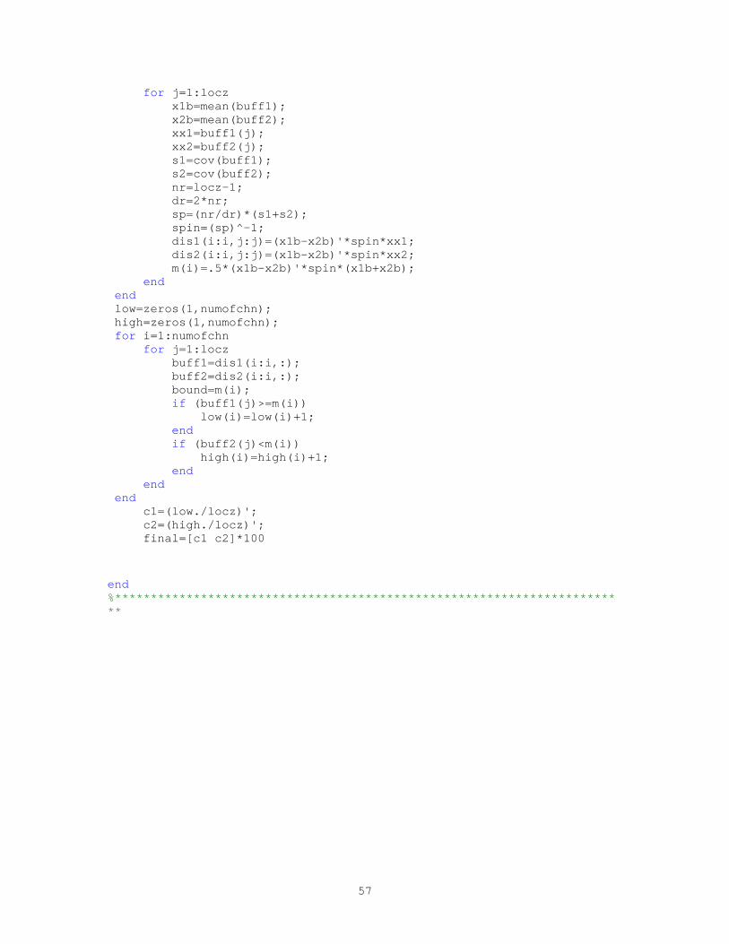
57

for j=1:locz x1b=mean(buff1); x2b=mean(buff2); xx1=buff1(j); xx2=buff2(j); s1=cov(buff1); s2=cov(buff2); nr=locz-1; dr=2*nr; sp=(nr/dr)*(s1+s2); spin=(sp)^-1; dis1(i:i,j:j)=(x1b-x2b)'*spin*xx1; dis2(i:i,j:j)=(x1b-x2b)'*spin*xx2; m(i)=.5*(x1b-x2b)'*spin*(x1b+x2b); end end

low=zeros(1,numofchn); high=zeros(1,numofchn); for i=1:numofchn

for j=1:locz buff1=dis1(i:i,:); buff2=dis2(i:i,:); bound=m(i); if (buff1(j)>=m(i)) low(i)=low(i)+1; end if (buff2(j)<m(i)) high(i)=high(i)+1; end end end

c1=(low./locz)'; c2=(high./locz)'; final=[c1 c2]*100

end %************************************************************************

58

Appendix D – Simulation of EEG with AR

Modeling(MATLAB Code)

%This program AR simulation.m is used for CSP verification purpose %The EEG signal is simulated using the AR parameters calculated from trial %G11E. %The parameter varied in this simulation is the variance of signals for %channels 1, 3 and 7 in the data set 2. %CSP method is applied on the simulated EEG data for verification of CSP. %The output of the program is the spatial patterns matrix of the data sets %created.

%-------------------------------------------------------------------------- clc clear all close all [filename]=uigetfile('*.mat','Choose file to load:'); load(filename); % Load the structure rawdata fprintf('\n') sf = 128; % sf has been lowered from the original 256 to 128 r = rawdata; clear rawdata; eegdata = [r.elec1 r.elec2 r.elec3 r.elec4 r.elec5 r.elec6 r.elec7 r.elec8 r.elec9... r.elec10 r.elec11 r.elec12 r.elec13 r.elec14 r.elec15 r.elec16 r.elec17... r.elec18 r.elec19 r.elec20 r.elec21]; datalabels = r.labels; fname1 = 'MATB-Cap19.locs'; data = eegdata(:,1:19); %***EEG data*** [xm,ym]=size(data); de=round(xm/2); f=0:64/de:64; f1=f./64; f1=f1(1:de); f1(de)=1; f(de)=1;

f=f(1:de); x=500;%***Number of samples in each channel*** ord=8;%***Order of the AR parameters*** E=[30 330 390 690 720 1020];%***Sequence of Trial G11E***

%***Computation of Generic AR parameters*** for i=1:19 dat=data(:,i:i);

59

ar(i:i,:)=arburg(dat,ord); end x=500; A=sum(ar)./19; %*****************************************

SL=zeros(7,x); SH=zeros(7,x); var1=[1.41 1 2 1 1 1 2.82]; %***Variance control applied*** var2=[1 1 1 1 1 1 1];

%***Simulation of EEG signals from white noise using AR modeling*** for i1=1:7

r=randn(1,x); rL(i1:i1,:)=var1(i1).*r; rH(i1:i1,:)=var2(i1).*r; end for i2=1:7

buffL=rL(i2:i2,:); buffH=rH(i2:i2,:);

for j2=1:x mlim1=j2-1; mlim2=j2-ord; if (mlim1<=0) SL(i2:i2,j2:j2)=buffL(j2); SH(i2:i2,j2:j2)=buffH(j2); end if(mlim2<=0) mlim2=1; end if (mlim1>0) buL=SL(mlim2:mlim1); buL=fliplr(buL); buH=SH(mlim2:mlim1); buH=fliplr(buH); len=length(buL); bL=A(1:len); bH=A(1:len); sum1=sum(buL.*bL)+buffL(j2); sum2=sum(buH.*bH)+buffH(j2); SL(i2:i2,j2:j2)=sum1; SH(i2:i2,j2:j2)=sum2; end end end

X1=SL; X2=SH; %*********************************************************************

%***Application of CSP for result verification disp('normalized data sets')

60

Ra= (X1*X1')/trace(X1*X1'); Rb= (X2*X2')/trace(X2*X2'); R=Ra+Rb; [Bc,L] = eig(R); disp('whitended data') W=(L)^-.5*(Bc)'; Sa=W*Ra*W'; Sb=W*Rb*W'; [U1,La]= eig(Sa); [U2,Lb]= eig(Sb); U=(U1); disp('projection matrix') P=(U2'*W); disp('spatial patterns') spt=abs(((P)^-1)) ; [m,n]=size(P); noc=2; lim1=noc-1; p1=P(1:m,1:noc); p2=P(1:m,(n-lim1):n); spt1=spt(1:m,1:noc); spt2=spt(1:m,(n-lim1):n); PP=[p1 p2]; Z1=(X1'*PP)'; Z2=(X2'*PP)'; [x,y]=size(Z1); [len,br]=size(spt1); for i=1:br buff1=spt1(1:len,i:i); buff2=spt2(1:len,i:i); for j=1:len if (max(buff1)==buff1(j)) ch1(i)=j; end if (max(buff2)==buff2(j)) ch2(i)=j; end end end

spt %*** Spatial patterns matrix %*******************************************************************

61

Appendix E – Simulation of EEG with IIR Modeling

(MATLAB Code)

%This program IIR_simulation.m is used for CSP verification purpose %The EEG signal is simulated using the IIR parameters calculated from trial %G11E. %The parameter varied in this simulation is the magnitude spectrum of signals for %channels 1, 3 and 7 in the data set 2. %The variance of all channels were normalized to 1 %CSP method is applied on the simulated EEG data for verification of CSP. %The output of the program is the spatial patterns matrix of the data sets %created.

%-------------------------------------------------------------------------- clc clear all close all [filename]=uigetfile('*.mat','Choose file to load:'); load(filename); % Load the structure rawdata fprintf('\n') sf = 128; % sf has been lowered from the original 256 to 128 r = rawdata; clear rawdata; eegdata = [r.elec1 r.elec2 r.elec3 r.elec4 r.elec5 r.elec6 r.elec7 r.elec8 r.elec9... r.elec10 r.elec11 r.elec12 r.elec13 r.elec14 r.elec15 r.elec16 r.elec17... r.elec18 r.elec19 r.elec20 r.elec21]; datalabels = r.labels; % noc=19; fname1 = 'MATB-Cap19.locs'; data = eegdata(:,1:19); %***EEG data*** [x,y]=size(data); de=round(x/2); f=0:1/de:1; f(de)=1; f=f(1:de); %***Computation of Generic IIR parameters***

for i=1:19 buff1=data(:,i:i); mag=abs(fft(buff1)); mag=mag(1:de); mag=mag./max(mag); [b1,a1]=yulewalk(8,f,mag'); b(i:i,:)=b1; a(i:i,:)=a1;

62

end B=sum(b)/19; A=sum(a)/19; %*********************************************** x=500;

%***Filtering the white noise with the estimated IIR parameters****** for i=1:7 r1=randn(1,x); r2=randn(1,x); rL(i:i,:)=filter(B,A,r1); rH(i:i,:)=filter(B,A,r2); end %*********************************************************************

%***Desired magnitude responses*************************************** f1=[0 .1 .9 1]; m1=[0 0 2 0]; [b1,a1]=yulewalk(8,f1,m1); h1=freqz(b1,a1,x); f3=[0 .1 .9 1]; m3=[0 0 4 0]; [b3,a3]=yulewalk(8,f3,m3); h3=freqz(b3,a3,x); f7=[0 .1 .9 1]; m7=[0 0 8 0]; [b7,a7]=yulewalk(8,f7,m7); h7=freqz(b7,a7,x);

for i=1:7; if (i==1) buff1=rH(i:i,:); rH(i:i,1:x)=filter(b1,a1,buff1); end if (i==3) buff3=rH(i:i,:); rH(i:i,1:x)=filter(b3,a3,buff3); end if (i==7) buff7=rH(i:i,:); rH(i:i,1:x)=filter(b7,a7,buff7); end end %************************************************************************ X2=rH; X1=rL; %***Normalization of the variance of the signals to 1******************** mult1=sqrt(var(X1')); mult2=sqrt(var(X2'));

63

for norm=1:7

buffz1=X1(norm:norm,:)./mult1(norm); X1(norm:norm,:)=buffz1; buffz2=X2(norm:norm,:)./mult2(norm); X2(norm:norm,:)=buffz2; end

%************************************************************************

%***Application of the CSP method for CSP validation********************** disp('normalized data sets') Ra= (X1*X1')/trace(X1*X1'); Rb= (X2*X2')/trace(X2*X2'); R=Ra+Rb; [Bc,L] = eig(R); disp('whitended data') W=(L)^-.5*(Bc)'; Sa=W*Ra*W'; Sb=W*Rb*W'; [U1,La]= eig(Sa); [U2,Lb]= eig(Sb); U=abs(U1); disp('projection matrix') P=(U1'*W); disp('spatial patterns') spt=abs(((P)^-1)) ; %***Spatial patterns matirx**** f=0:64/250:64; f=f(1:250); f(250)=64;

figure p1=abs(fft(X1(2,:))); p1=p1(1:250); plot(f,p1) xlabel('normalized frequency, no units') ylabel('amplitude response magnitude') title('data1 channel 2') figure p2=abs(fft(X2(2,:))); p2=p2(1:250); plot(f,p2) xlabel('normalized frequency, no units') ylabel('amplitude response magnitude') title('data2 channel 2')

figure

64

g=abs(fft(X1(1,:))); g=g(1:250); plot(f,g) xlabel('normalized frequency, no units') ylabel('amplitude response magnitude') title('data1 channel ') figure d=abs(fft(X2(1,:))); d=d(1:250); plot(f,d) xlabel('normalized frequency, no units') ylabel('amplitude response magnitude') title('data2 channel 1') figure q=abs(fft(X1(3,:))); q=q(1:250); plot(f,q) xlabel('normalized frequency, no units') ylabel('amplitude response magnitude') title('data1 channel 3 ') figure w=abs(fft(X2(3,:))); w=w(1:250); plot(f,w) xlabel('normalized frequency, no units') ylabel('amplitude response magnitude') title('data2 channel 3') figure p=abs(fft(X1(7,:))); p=p(1:250); plot(f,p) xlabel('normalized frequency, no units') ylabel('amplitude response magnitude') title('data1 channel 7') figure l=abs(fft(X2(7,:))); l=l(1:250); plot(f,l) xlabel('normalized frequency, no units') ylabel('amplitude response magnitude') title('data2 channel 7')

65

Appendix F – Optimal Channel Selection Using CSP(MATLAB Code)

%This program CSP.m selects 5 optimal channels by calculating the spatial patterns matrix of the data extracted from the optimal rhythm. %The data from all trials are accepted automatically. %The output of the program is a final set of optimal channels considering all the trials. %The Channels used for EEG data acquisition is shown below. %FP1(1),FP2(2),F7(3),F3(4),FZ(5),F4(6),F8(7),T3(8),T5(9),C3(10),CZ(11),C4(12),T4(13),T6(14),P3(15),PZ(16),P4(17),O1(18),O2(19).

% ------------------------------------------------------------------------- clc clear all close all chnap=zeros(15,19); band=input('enter the band to be analyzed as del the alp or bet with in single quotes ')

%**Loop for accpeting data from al trials**** for sek=1:15 seqz=['E' 'F' 'D' 'B' 'A' 'E' 'C' 'F' 'D' 'B' 'C' 'F' 'A' 'B' 'C']; fil=['G11Eraw'; 'G12Fraw'; 'G13Draw'; 'G21Braw'; 'G22Araw'; 'G23Eraw'; 'G31Craw'; 'G32Fraw'; 'G33Draw'; 'G41Braw'; 'G42Craw'; 'G43Fraw' ; 'G51Araw'; 'G52Braw'; 'G53Craw']; filename=fil(sek:sek,1:7); seq=seqz(sek); chcnt=zeros(1,19); chndisp=zeros(1,6); load(filename); fprintf('\n') sf = 128; % sampling frequency in Hz r = rawdata; clear rawdata; eegdata = [r.elec1 r.elec2 r.elec3 r.elec4 r.elec5 r.elec6 r.elec7 r.elec8 r.elec9... r.elec10 r.elec11 r.elec12 r.elec13 r.elec14 r.elec15 r.elec16 r.elec17... r.elec18 r.elec19 r.elec20 r.elec21]; datalabels = r.labels; fname1 = 'MATB-Cap19.locs'; data = eegdata(:,1:19); %**EEG data**

%**Normalizing the EEG data of all channels to equal variance**** mulz=sqrt(var(data)); for norm=1:19 buffznorm=data(:,norm:norm); data(:,norm:norm)=buffznorm./mulz(norm); end %*****************************************************************

66

A=[30 330 360 660 690 990]; B=[30 330 390 690 720 1020]; C=[30 330 360 660 720 1020]; D=[30 330 360 660 720 1017]; E=[30 330 390 690 720 1020]; F=[30 330 360 660 690 990];

%***Extraction of data according to the code of sequence********* switch(seq)

case('A') datL=data(A(1)*sf:A(2)*sf,:); datM=data(A(3)*sf:A(4)*sf,:); datH=data(A(5)*sf:A(6)*sf,:); case('B') datL=data(B(1)*sf:B(2)*sf,:); datH=data(B(3)*sf:B(4)*sf,:); datM=data(B(5)*sf:B(6)*sf,:); case('C') datM=data(C(1)*sf:C(2)*sf,:); datL=data(C(3)*sf:C(4)*sf,:); datH=data(C(5)*sf:C(6)*sf,:); case('D') datM=data(D(1)*sf:D(2)*sf,:); datH=data(D(3)*sf:D(4)*sf,:); datL=data(D(5)*sf:D(6)*sf,:); case('E') datH=data(E(1)*sf:E(2)*sf,:); datL=data(E(3)*sf:E(4)*sf,:); datM=data(E(5)*sf:E(6)*sf,:); case('F') datH=data(F(1)*sf:F(2)*sf,:); datM=data(F(3)*sf:F(4)*sf,:); datL=data(F(5)*sf:F(6)*sf,:); end %********************************************************************

%***Segmenting the data into 10 second windows*********************** win=10; %***lenght of the hamming window in seconds****************** lap=5; %***Overlap of the hamming windows in seconds**************** diff=win-lap; lim1=1; lim2=10; li1=1;

maxlim=1; [x,y]=size(datL); locz=0;

while (maxlim<x) locz=locz+1;

67

datL1=datL(lim1:(lim2*sf),:); datH1=datH(lim1:(lim2*sf),:); datM1=datM(lim1:(lim2*sf),:); li1=li1+diff; lim1=li1*sf; lim2=lim2+diff; maxlim=lim2*sf; if (maxlim>=x) datL1=datL(lim1:x,:); datH1=datH(lim1:x,:); datM1=datM(lim1:x,:); end [x1,y1]=size(datL1); fL=zeros(1:x1,1:1); fH=zeros(1:x1,1:1); fM=zeros(1:x1,1:1); alp=[8 13]/64; bet=[18 26]/64; del=[.5 4]/64; the= [4 8]/64; [x1,y1]=size(datL1); for hum=1:19 datL1(1:x1,hum:hum)=datL1(1:x1,hum:hum).*hamming(x1); datH1(1:x1,hum:hum)=datH1(1:x1,hum:hum).*hamming(x1); end

%**********Extraction of data from each rhythm****************** switch(band)

case('alp') ban=alp; case('bet') ban=bet; case('the') ban=the; case('del') ban=del;

case('full') X1=datL1'; X2=datH1'; end

[b,a]=ellip(4,6,50,ban); X1=filter(b,a,datL1); X2=filter(b,a,datH1);

X1=X1'; X2=X2'; %************************************************************* %***Application of the CSP method*****************************

68

%disp('normalized data sets') Ra= (X1*X1')/trace(X1*X1'); Rb= (X2*X2')/trace(X2*X2'); R=Ra+Rb; [Bc,L] = eig(R); %disp('whitended data') W=(L)^-.5*(Bc)'; Sa=W*Ra*W'; Sb=W*Rb*W'; [U1,La]= eig(Sa); [U2,Lb]= eig(Sb); %disp('projection matrix') P=U1'*W; %disp('spatial patterns') spt=abs((P)^-1) ; [x2,y2]=size(spt); noc=5; dat1=spt(1:x2,1:noc); [x3,y3]=size(dat1);

for i1=1:y3 buff1=dat1(1:x3,i1:i1);

for j1=1:x3 if (max(buff1)==buff1(j1)) ch1(i1)=j1; end

end end cha(locz:locz,:)=ch1;

end chcnt=zeros(1,19); [x4,y4]=size(cha); for i2=1:y4

buff2=cha(1:x4,i2:i2);

for j2=1:x4 for z1=1:x4 if (buff2(z1)==j2) chcnt(j2)=chcnt(j2)+1; end

end end end

chcnt; sm=chcnt; big=sort(sm,'descend');

69

yz=1; yx=find(sm==big(1)); yz=[yz yx];

for u=2:5 num1=big(u); num2=big(u-1); if(num1==num2) else yx=find(sm==num1); yz=[yz yx]; end gg=length(yz); end yz=yz(1:1,2:gg); gg1=length(yz); chnap(sek:sek,1:gg1)=yz; end chnap(13:13,3:19)=0; chnap(14:14,3:19)=0;

fincnt=zeros(1,19); for ii=1:19 numz=ii; for jj=1:15 buff=chnap(jj:jj,:); for zz=1:19 if (buff(zz)==numz); fincnt(ii)=fincnt(ii)+1; end end end end fincnt%***Optimal channels selected*************************************** %*************************************************************************

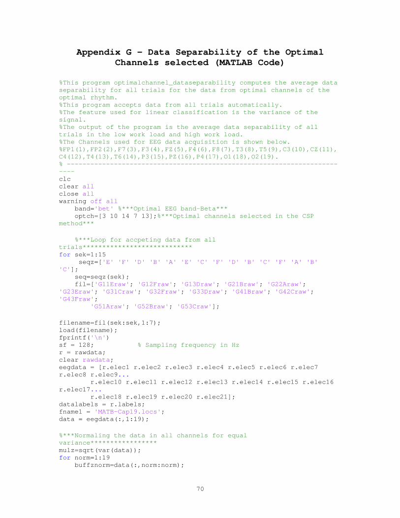
70

Appendix G – Data Separability of the Optimal

Channels selected (MATLAB Code)

%This program optimalchannel_dataseparability computes the average data separability for all trials for the data from optimal channels of the optimal rhythm. %This program accepts data from all trials automatically. %The feature used for linear classification is the variance of the signal. %The output of the program is the average data separability of all trials in the low work load and high work load. %The Channels used for EEG data acquisition is shown below. %FP1(1),FP2(2),F7(3),F3(4),FZ(5),F4(6),F8(7),T3(8),T5(9),C3(10),CZ(11),C4(12),T4(13),T6(14),P3(15),PZ(16),P4(17),O1(18),O2(19). % ------------------------------------------------------------------------- clc clear all close all warning off all band='bet' %***Optimal EEG band-Beta*** optch=[3 10 14 7 13];%***Optimal channels selected in the CSP method*** %***Loop for accpeting data from all trials**************************** for sek=1:15 seqz=['E' 'F' 'D' 'B' 'A' 'E' 'C' 'F' 'D' 'B' 'C' 'F' 'A' 'B' 'C']; seq=seqz(sek); fil=['G11Eraw'; 'G12Fraw'; 'G13Draw'; 'G21Braw'; 'G22Araw'; 'G23Eraw'; 'G31Craw'; 'G32Fraw'; 'G33Draw'; 'G41Braw'; 'G42Craw'; 'G43Fraw'; 'G51Araw'; 'G52Braw'; 'G53Craw']; filename=fil(sek:sek,1:7); load(filename); fprintf('\n') sf = 128; % Sampling frequency in Hz r = rawdata; clear rawdata; eegdata = [r.elec1 r.elec2 r.elec3 r.elec4 r.elec5 r.elec6 r.elec7 r.elec8 r.elec9... r.elec10 r.elec11 r.elec12 r.elec13 r.elec14 r.elec15 r.elec16 r.elec17... r.elec18 r.elec19 r.elec20 r.elec21]; datalabels = r.labels; fname1 = 'MATB-Cap19.locs'; data = eegdata(:,1:19);

%***Normaling the data in all channels for equal variance***************** mulz=sqrt(var(data)); for norm=1:19 buffznorm=data(:,norm:norm);

71

data(:,norm:norm)=buffznorm./mulz(norm); end %************************************************************************* A=[30 330 360 660 690 990]; B=[30 330 390 690 720 1020]; C=[30 330 360 660 720 1020]; D=[30 330 360 660 720 1017]; E=[30 330 390 690 720 1020]; F=[30 330 360 660 690 990];

%***Extracting data from the optimal channels****************************** chnnum=length(optch); for chn=1:1

opcnum=optch(1:chnnum); for i=1:chnnum cnum1=opcnum(i); data1(:,i:i)=data(:,cnum1:cnum1); end %**************************************************************************

%***Extraction of data based on the code of sequence********************** switch(seq)

case('A') datL=data1(A(1)*sf:A(2)*sf,:); datM=data1(A(3)*sf:A(4)*sf,:); datH=data1(A(5)*sf:A(6)*sf,:); case('B') datL=data1(B(1)*sf:B(2)*sf,:); datH=data1(B(3)*sf:B(4)*sf,:); datM=data1(B(5)*sf:B(6)*sf,:); case('C') datM=data1(C(1)*sf:C(2)*sf,:); datL=data1(C(3)*sf:C(4)*sf,:); datH=data1(C(5)*sf:C(6)*sf,:); case('D') datM=data1(D(1)*sf:D(2)*sf,:); datH=data1(D(3)*sf:D(4)*sf,:); datL=data1(D(5)*sf:D(6)*sf,:); case('E') datH=data1(E(1)*sf:E(2)*sf,:); datL=data1(E(3)*sf:E(4)*sf,:); datM=data1(E(5)*sf:E(6)*sf,:); case('F') datH=data1(F(1)*sf:F(2)*sf,:); datM=data1(F(3)*sf:F(4)*sf,:); datL=data1(F(5)*sf:F(6)*sf,:);

72

end

%*************************************************************************

%***Segmentation of data into 10 second segments************************** win=10; lap=5; diff=win-lap; lim1=1;

lim2=10; li1=1; maxlim=1; [x,y]=size(datL); locz=0;

while (maxlim<x) locz=locz+1; datL1=datL(lim1:(lim2*sf),:); datH1=datH(lim1:(lim2*sf),:); datM1=datM(lim1:(lim2*sf),:); li1=li1+diff; lim1=li1*sf; lim2=lim2+diff; maxlim=lim2*sf; if (maxlim>=x) datL1=datL(lim1:x,:); datH1=datH(lim1:x,:); datM1=datM(lim1:x,:); end [x1,y1]=size(datL1);

for hum=1:chn datL1(1:x1,hum:hum)=datL1(1:x1,hum:hum).*hamming(x1); datH1(1:x1,hum:hum)=datH1(1:x1,hum:hum).*hamming(x1); end

switch(band) case('alp') ban=alp; case('bet') ban=bet;

case('the') ban=the;

case('del') ban=del;

case('full')

73

X1=datL1'; X2=datH1'; end

[b,a]=ellip(4,6,50,ban); X1=filter(b,a,datL1); X2=filter(b,a,datH1); X1=X1'; X2=X2'; fet1b(locz:locz,1:chnnum)=log(var(X1'));%**Feature samples of low work load fet2b(locz:locz,1:chnnum)=log(var(X2'));%*Feature samples of high work load end

%***Design of Linear classifier and computation of data separability******

x1b=mean(fet1b); x2b=mean(fet2b); s1=cov(fet1b); s2=cov(fet2b); sp=.5*(s1+s2); spin=(sp)^-1; m=.5*(x1b'-x2b')'*spin*(x1b'+x2b'); dis1=(x1b'-x2b')'*spin*fet1b'; dis2=(x1b'-x2b')'*spin*fet2b'; class1=zeros(1,locz); class2=zeros(1,locz); for cmp=1:locz if (dis1(cmp)>=m) class1(cmp)=class1(cmp)+1; end if (dis2(cmp)<m) class2(cmp)=class2(cmp)+1; end end classl(sek,chn,1)=(sum(class1)/locz)*100; classh(sek,chn,1)=(sum(class2)/locz)*100; clear data1 end

end clear x1

low=sum(classl)/15 high=sum(classh)/15 %*************************************************************************

optimal eeg channels and rhythm selection for task

Documents