FINAL REPORT

NAG- 1-01087

OPTIMAL EXPERIMENT DESIGN FOR THERMAL CHARACTERIZATION OF FUNCTIONALLY GR4DED MATERIALS.

Submitted to Dr. Max Blosser NASA Langley Research Center Metals and Structures Branch

August 18, 2003

Kevin D. Cole Mechanical Engineering Department University of Nebraska-Lincoln

kcolel @unl.edu

, c 402-472-5857

Abstract

The purpose of the project was to investigate methods to accurately verify that designed ,

materials meet thermal specifications. The project involved heat transfer calculations and optimization studies, and no laboratory experiments were performed. One part of the research involved study of materials in which conduction heat transfer predominates. Results include techniques to choose among several experimental designs, and protocols for determining the optimum experimental conditions for determination of thermal properties. Metal foam materials were also studied in which both conduction and radiation heat transfer are present. Results of this work include procedures to optimize the design of experiments to accurately measure both conductive and radiative thermal properties. Detailed results in the form of three journal papers have been appended to this report.

k

https://ntrs.nasa.gov/search.jsp?R=20040004381 2018-06-02T00:59:00+00:00Z

Introduction Research on functionally graded materials has been underway for several years.

Functionally graded materials include composites with epoxy and metal matrices; metal foams; and any built-up material or structure with properties designed to vary across the structure. In the future, as functionally graded materials are incorporated into aerospace structures, part of the procurement process will involve certification that the materials meet the specifications. However, there has been little research on accurate thermal characterization of functionally graded materials. The present project is a first step towards closing this gap in the procurement cycle by developing accurate methods to measure the thermal properties of functionally graded (FG) materials.

variation of thermal conductivity and specific heat were studied. If the maximum (simulated) temperature is kept low, the primary mechanism for heat transfer is conduction (molecule-to-molecule diffusion). Simulated experiments were studied that involved transient heating, and also steady-periodic heating. Second, metal foams were studied for which both conduction and radiation are important in the transfer of heat. Metal-foam materials are being studied as possible components of aerospace thermal protection systems (TPS).

given. Detailed results are given in the appendix in the form of research papers.

Two classes of materials were studied in this project. First, materials with spatial

In this report, a brief account of the results of each of three phases of the study is

Conduction-dominated material, transient heating

measurement of thermal properties in FG materials with spatially-varying thermal properties. The maximum (simulated) temperature rise was limited to about 40 C s o that conduction would be the dominant mechanism for heat transfer.

One-dimensional transient experiments were studied for a material with linearly- varying thermal properties described by parmeters E, k , and spatial slope e. Variation of properties with temperature was not treated. Several transient experimental designs were considered, including single or multiple heating events and including surface and/or interior temperature sensors. An optimality criterion D, based on sensitivity coefficients [ 11 was used to find the best operating conditions for each experiment, and to find the best experimental design among those studied.

parameters when spatial slope e is small compared to when e is large; that is, it is easier to "see" large spatial variations in properties. The best experimental design involves analysis of combined data from two separate heating events, one with heating on one side of the body and one with heating on the other side, each time with the sensor located on the heated side and the unheated side maintained at a fixed temperature. This conclusion is also supported by a series of simulated experiments, carried out with regression analysis of error-containing temperature values. The optimai operating conditions for the experiment are somewhat dependent on the property slope e. Detailed results are given in Appendix A.

The first phase of the research involved transient-heating experiments for the

The results of the optimality study show that it is more difficult to obtain accurate

Conduction-dominated material, steady-periodic heating This phase of the research investigated steady-periodic methods for thermal

characterization of functionally graded materials. Specifically, the work was carried out to explore, via numerical simulation, the use of photothermal methods. A new heat transfer model was developed for the response of layered material to periodic heating, based on the method of Green's functions, which is numerically better behaved than previous work. The method was applied to a Si02 layer on silicon and compared to literature values [2] to validate the method. The optimality criterion 0, introduced earlier, indicates which frequency range of experimental data should provide the best possible estimates of the layer conductivity and contact conductance.

functionally-graded material with a power-law distribution of thermal properties, This type of material was studied previously for its thermal-stress behavior [3]. The results indicate that largest temperature response is found by heating the sample on the l o w 4 side, and the phase of the temperature is particularly important for estimation of thermal properties. Component conductivities kl and kz have similar-shaped sensitivity coefficients, and consequently both cannot be estimated simultaneously from experimental data. The most important parameter is power-law exponent p which describes the spatial distribution of thermal properties in the functionally-graded material. Values for optimality criterion D indicate that values for p may be found simultaneously with one of the conductivities, but not both. Dimensionless frequencies less than unity are important for measurement of spatial-distribution parameter p . The magnitude of the optimality criterion D also suggests that it will be easier to estimate parameters for p =1 (near-linear spatial variation) compared to other values ofp. More detailed results are given in Appendix B.

The new steady-periodic model was then applied to a two-component

Metal Foams with conduction and radiation heat transfer

In this phase of the research the methods of optimal experiment design are applied to a high-porosity nickel foam material, with thermal property values taken from Sullins and Daryabeigi [4]. Contained within the model are five parameters considered to b e intrinsic properties of the material that must be determined empirically. Two of these intrinsic properties are related to heat transfer by conduction and three are related to the radiative heat transfer. The intrinsic properties are the following: F, the efficiency for solid (metal) conductivity; a, coupling coefficient for solid-gas conductivity; eo and el, parameters defining the temperature-dependent specific extinction coefficient as e = eo + el T; and, GI, the albedo of scattering.

simulated experiments have been studied to determine which experimental conditions provide the best estimates of the thermal properties.

heating event that could be used to determine the radiation and conduction parameters. Strict use of the D parameter leads to experiments that were somewhat too short in t he sense that more accurate parameter estimates could be obtained from simulated data sets of longer duration. By considering the conduction and radiation behavior of the model, a

Based on a one-dimensional model of transient heat transfer, a large number of

kiaximization of the optimdity criterion D leads to an experiment ccntaining one

set of two shorter heating events were found that provided more accurate parameter estimates.

the simulated experiments. The coupling coefficient, 'a ', was the most difficult parameter to determine accurately, in part because its sensitivity coefficient is similar in shape to that of the other conduction parameter, F. This indicates that the conduction parameters are close to linearly dependent. Coupling coefficient ' a ' was an ad-hoc parameter added to Sullins' model in order to obtain better agreement with experimental data at high pressures. This suggests that there may be a different pair of conduction parameters that could adequately model the conduction process and provide more robust estimation than exhibited here. Complete results are given in Appendix C.

The radiation parameter w was easily found to a high degree of accuracy b y all of

Conclusions.

Optimality criterion D is an important tool for exploring possible experimental conditions at little computational cost. Criterion D, however useful, is not sufficient to determine how well an experiment design will actually perform. Estimation of the parameters from simulated experimental data, or, from actual laboratory experiments, .is required to quantify the experimental accuracy.

Optimal experiment design involves criterion D which is computed from sensitivity coefficients. Sensitivity coefficients are required anyway as part of the data analysis to extract thermal properties from experimental data. Thus, although some time and effort are required for optimal experimental design, no new computational tools are required.

The methods of optimal experiment design presented in this report are general and apply to different materials, different experimental techniques, and different experimental conditions. Careful use of the techniques of optimal experiment design will decrease the amount of time needed in the laboratory and increase the accuracy of thermal property estimates.

References

1. Taktak, R., Beck, J. V., and Scott, E. P., "Optimal experimental design for estimating thermal properties of composite materials," International Journal of Heat and Mass Transfer, Vol. 36, No. 12, 1993, pp. 2977-2986.

2. H. Hu, X. Wang, and X. Xu, Generalized theory of the photoacoustic effect i n a multilayer material", J. of Applied Physics, 86:7, 3953-3958 (1999).

3. Z. H. Jin and G. H. Paulino, "Transient thermal stress analysis of an edge crack in a functionally graded material", International J. of Fracture, 107, 73-98 (2001).

4. Sullins, A. D., and Daryabeigi, K., "Effective Thermal Conductivity of High Porosity Open Cell Nickel Foam, " Proceeding of the 35th AIAA Thermophysics Conference, Anaheim CAY June 11 -14,200 1, paper AIAA 200 1-28 19.

APPENDIX A.

Thermal Characterization of Functionally Graded Materials-Design of Optimal Experiments, submitted July 2003 to the AIAA J. of Thermophysics and Heat Transfer.

THERMAL CHARACTERIZATION O F FUNCTIONALLY

GRADED MATERIALS- DESIGN OF OPTIMUM EXPERIMENTS *

Kevin D. Cole t Mechanical Engineering Department, University of Nebraska

N104 Walter Scott Engineering Center, Lincoln, Nebraska 68588-0656 USA

Abstract

This paper is a study of optimal experiment design applied to the measure of thermal properties in functionally graded materials. As a first step, a material

with linearly-varying thermal properties is analyzed, and several different tran-

sient experimental designs are discussed. An optimality criterion, based on sen-

sitivity coefficients, is used to identify the best experimental design. Simulated

experimental results are analyzed to verify that the identified best experiment

design has the smallest errors in the estimated parameters. This procedure is

general and can be applied to design of experiments for a variety of materials.

- *submitted July 18, 2003 to the AIAA Journal of Thermophysics and Heat Transfer, ac-

t Associate Professor. member AIAA. cepted November 17, 2003.

1

Nomenclature

bk

C D e

IC L n

P Qo S

t T 2

X X

kth parameter

specific heat per unit volume, [J(m3K)-'] optimality condition, Eq. (12) slope of spatial variation, unitless

thermal conductivity [ W ( T ~ K ) - ~ ] sample thickness, [m]

number of time steps

number of parameters

applied heat flux, [W m-2]

number of sensors

time, [ S I temperature, [K] spatial coordinate [m] sensitivity coefficient, Eq. (9) sensitivity matrix [sn x p ]

Greek a thermal dsusivi ty [m2s-'] E

p density [kg m-3] 8 dimensionless time

small value for finite difference

h heater

a index for time step

j index for sensors

IC index for parameters

Superscripts - ( ) spatial average quantity

( )+ dimensionless quantity

2

Introduction

Functionally graded materials are being studied as possible components of aero-

space thermal protection systems. Functionally graded (FG) materials include

composites with epoxy and metal matrices, metal foams, or any structure with

properties designed to vary with position. In the future when FG materials

are specified as part of a vehicle program, part of the procurement process will

involve certification that the material meets the specifications.

To date there has been little research on accurate thermal characterization of

FG materials. The present research is intended to close this gap in the procure-

ment cycle by developing accurate methods to measure the thermal properties

of FG materials.

A review of the pertinent literature is given next. The focus here is on

FG materials described by macroscopic or effective properties, rather than on

microscopic structures. Several researchers have found exact analytical so- lutions for thermal response by representing a FG material as composed of

multiple layers each with different, spatially uniform, thermal properties1i2,

or with exponential-function variation of thermal properties along one spatial

direction3i4. Still others have used Galerkin's method to find temperature in

materials with arbitrary property distributions5. The primary motivation for

these studies of temperature has been to determine the thermal stresses. There

has also been some work to find the distribution of thermal properties tha t

optimizes the thermal stress distribution6i7.

There is only one research group that has reported experiments t o measure

thermal properties in a FG material. Maltino and Noda have used transient the-

ory applied to a FG material with exponential variation of thermal proper tie^'?^. They have measured the single parameter that describes the thermal property

variation in the material with a transient heating experiment. Their data anal-

ysis combines a single temperature datum with their transient theory to provide

a single value for the parameter. Although simple in concept, this approach is

sensitive to measurement noise.

The approach used in the present work is parameter estimation, a statistics-

based method of property measurement, that has been applied to transient

experiments for many yeardo. In this method the desired parameters are found

by non-linear regression between the experimental data (temperatures in this

case) and a computational model of the experiment. Parameter estimation

3

concepts have recently been applied to optimal experiment design for thermal

characterization of uniform materials11i12 and for materials with temperature

varying properties13.

The focus of this paper is to develop optimal experiments to thermally char-

acterize FG materials with low thermal conductivity. To the author’s knowledge

this is the first study of optimal experiments for thermal properties in FG ma-

terials.

Next a brief overview of the paper is given. In the next section a heat

transfer model of the one-dimensional FG material is described. The sensitivity

coefficients and sensitivity matrix are then defined, and their use in the design of

optimal experiments is described. Several experimental designs are investigated

for a material with linearly- varying thermal properties under specific (simu-

lated) experimental conditions. The best experimental design and the optimal

operating conditions are identified. The results are also verified with simulated

experiments for estimation of thermal parameters from noise-containing data.

Model

In this section a one-dimensional heat conduction model of the FG material is

discussed. This model is used to both simulate the experiments and to construct

the sensitivity coefficient matrix.

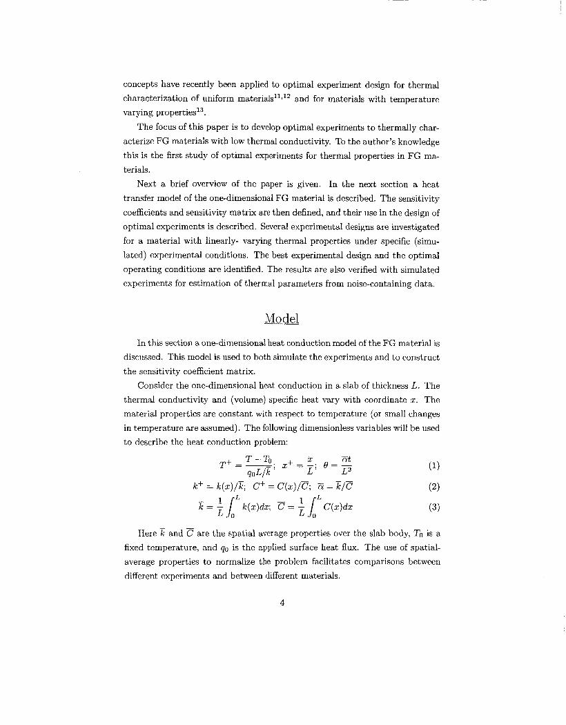
Consider the one-dimensional heat conduction in a slab of thickness L. The

thermal conductivity and (volume) specific heat vary with coordinate z. The

material properties are constant with respect to temperature (or small changes

in temperature are assumed). The following dimensionless variables will be used

to describe the heat conduction problem:

k+ = k ( z ) / Z ; c+ = C(z)/C; 7% = E/C (2)

(3) L - L -

k = ; L k(z)dz; c= ;1 C(z)dx Here % and are the spatial average properties over the slab body, TO is a

fixed temperature, and qo is the applied surface heat flux. The use of spatial-

average properties to normalize the problem facilitates comparisons between

different experiments and between different materials.

4

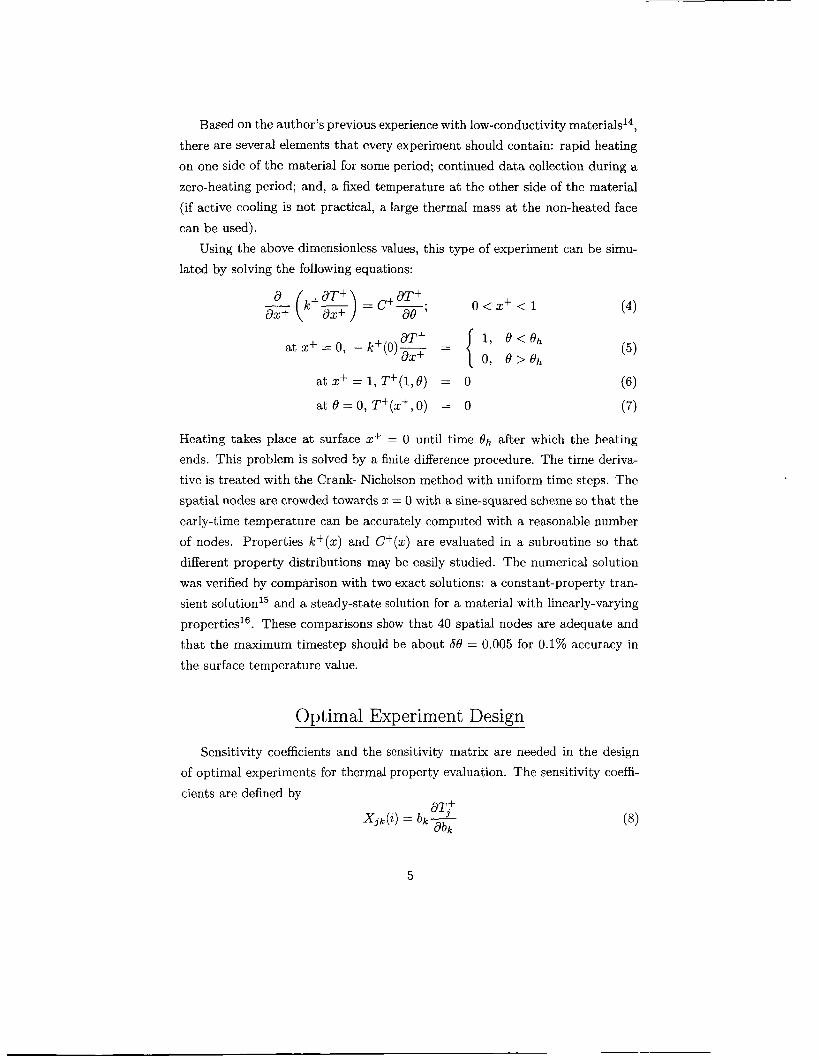
Based on the author’s previous experience with low-conductivity materials14,

there are several elements that every experiment should contain: rapid heating

on one side of the material for some period; continued da ta collection during a

zero-heating period; and, a fixed temperature at the other side of the material

(if active cooling is not practical, a large thermal mass at the non-heated face

can be used).

Using the above dimensionless values, this type of experiment can be simu-

lated by solving the following equations:

o < z + < 1 d dT+ dT+

LIT+ at z+ = 0, - k+(o)- ax+

1, 8 < 0, 8 > O h

=

at z+ = 1, Tf( i , e ) = o at e = 0, T+(x+,o) = o

(4)

(5)

Heating takes place a t surface IC+ = 0 until time Oh after which the heating

ends. This problem is solved by a finite difference procedure. The time deriva-

tive is treated with the Crank- Nicholson method with uniform time steps. The

spatial nodes are crowded towards x = 0 with a sine-squared scheme so tha t the

early-time temperature can be accurately computed with a reasonable number

of nodes. Properties k + ( z ) and Ct(z) are evaluated in a subroutine so that

different property distributions may be easily studied. The numerical solution

was verified by comparison with two exact solutions: a constant-property tran-

sient solution15 and a steady-state solution for a material with linearly-varying

properties16. These comparisons show that 40 spatial nodes are adequate and

that the maximum timestep should be about 68 = 0.005 for 0.1% accuracy in

the surface temperature value.

Optimal Experiment Design

Sensitivity coefficients and the sensitivity matrix are needed in the design

of optimal experiments for thermal property evaluation. The sensitivity coeffi-

cients are defined by

5

which is the sensitivity for the kth parameter, the j t h temperature sensor, and

the i t h time step. Parameters bk may include conductivity, specific neat, density,

etc. In this research the sensitivity matrix may encompass several heating events

considered together as one experiment, in which case additional heating events

are treated as additional sensors.

The sensitivity coefficients were computed with a finite-difference procedure

to approximate the derivative, as follows:

Here TG is the temperature a t the ith timestep for the j t h sensor. The value

of E = 0.001 was found to give well-behaved values for X . Much can be gained from studying the sensitivity coefficients to guide the

design of a n experiment, and there are two specific requirements that the sen-

sitivity coefficients must satisfy. First, the sensitivity coefficients should be as large as possible. Generally any change in the experiment tha t increases the size

of the sensitivity coefficient is an improvement. Second, when two or more pa-

rameters are to be measured in the same experiment, the sensitivity coefficients

must be linearly independent. That is, the shape of the sensitivity coefficients

must be different. A formal procedure to quantify these two requirements is

given next.

The sensitivity coefficients are assembled into a sensitivity matrix X , defined

by

Optimum experiment design is based on maximization of a quantity con-

structed from the sensitivity matrix multiplied by its transpose, given formally

6

by X T X . The elements of [p x p ] matrix X T X are given by

The optimality criterion selected for this study is the (normalized) determinant

of matrix X T X , given by

Note tha t the optimality criterion D is normalized by the maximum tempera-

ture rise (squared), the number of sensors, and the number of time steps. This is

important so tha t the optimality criterion D may be used to compare different

experiments. The determinant is computed for any value of p with well-known

matrix methods17. The optimality criterion insures that the sensitivity coeffi-

cients will be large and linearly independent.

The optimality criterion is subject t o the following standard statistical as-

sumptions: additive, uncorrelated errors with zero mean and constant variance;

errorless independent variable; and, no prior information. Maximizing the op-

timality criterion minimizes the hypervolume of the confidence region of the

parameter estimated3.

Experiment a1 Designs Considered

The focus of this research is to explore the design of experiments for ther-

mal characterization of functionally graded materials, that is, materials with

spatially-varying thermal properties.

As a first step, a material with linearly varying properties was analyzed.

Consider a one-dimensional slab body (0 < J: < L ) of this material. The thermal

conductivity [W(mK)-l] and volume specific heat [J(m3K)-'] are given by

k(z) = x[l + e . ( z / L - 1/2)]

C(z) = ??[I t e . ( Z / L - 1/2)]

Here the parameters are E, the spatial-average thermal conductivity, E, the

spatial-average specific heat, and e, the dimensionless slope. The same slope is

used for both k and C to represent the effect of density variation on thermal

properties in a metal foam, for example.

7

b h Q x 0" b

2

1.5

1

0.5

0

0 0.2 0.4 0.6 0.8 1 XR

Figure 1: Spatial variation of thermal properties studied.

A finite-difference computer routine was written to compute temperature,

sensitivity coefficients, and optimality criterion D. Three levels of spatial-property

spatial variation were studied: e = 0.2, 1.0, and 1.8, representing property varia-

tion of *lo%, k50%, and 3 ~ 9 0 % ~ respectively, from the mean value, as shown in

Fig. 1. Different mean values for were not studied since the normalized

results are valid for any conductivity and specific heat.

and

Several combinations of simulated experimental conditions were studied, in-

cluding the number of and location of sensors, heating on one side or the other,

heating duration, experiment duration, and the number of parameters.

Results for Opt imality

The results for optimality condition D are given in this section. The special

case when the thermal properties are spatially constant is considered first for

comparison with earlier work. There are only two parameters present, and

C. Consider an experiment with a single on-off heating event and with one

temperature sensor located on the heated surface. The normalized optimality

condition for this case is plotted versus dimensionless time in Fig. 2 for several

different heater-off times. This figure reproduces the results of Taktak et al.ll

t o provide verification of the code used for the present research. Note in Fig. 2 that continuous heating creates a single baseline value for each case, and then

when heating stops the D-value jumps above this baseline by a factor of two or so. The optimal experiment for a uniform-property material involves a heating

duration of Oh = 2.25 and experiment duration about 3.0 where D,,, = 0.02.. In the next sections materials with linearly-varying properties will be discussed.

-

8

0.02 1

0

4 0.016

- 2.0 - 1.0

I I I I , I I

1 2 0.012

s I-

' 0.008 1 0.004

I

0 1 2 3 4

a t / ~ 2

Figure 2: Optimality condition D for a uniform property material for estimat-

ing parameters and for several values of heater-off time Oh. There is one

temperature sensor a t x = 0 and heating at x = 0.

One heating event, one sensor.

In this section a material with linear properties described by Eqs. (13) and (14) is studied for which the three parameters are k, C, and e. Consider a simulated

experiment containing a single heating event and a single sensor a t the heated

surface. The other surface is maintained a t ambient temperature. Consider first

continuous heating to investigate the baseline values of D. In Fig. 3 optimality

condition D is plotted versus time for three values of slope e for a material

heated at x = 0 (the low-k side). The central result shown in Fig. 3 is tha t

the baseline D-values for three parameters are orders of magnitude less than for two parameters shown in Fig. 2. Clearly is it more difficult to estimate three

parameters compared with two. Another observation is that the magnitude of

D is smaller for smaller values of slope e. Thus it is more difficult to estimate

small values of e for which the properties are nearly uniform.

- _

Next consider Fig. 4 in which D-values are shown for the same materials

9

A I E-006

2 1E-007

a, -0 lE-oo81 1

- 1.0 - - 1E-009: I I I I 0.2 I I , I I I

0 2 4 6 8 10 o l t l L 2

Figure 3: Optimality condition D for a linearly-varying property material with

continuous heating a t 3: = 0 and one sensor a t x = 0. Parameters are IC, C, and

e.

- -

but with the experiment reversed: continuous heating at x = L (the high-k

side); a single temperature sensor at x = L; and, a fixed temperature a t x = 0. For e = 0.2 the D-values are similar in size and shape to Fig. 3. For e = 1.0 the peak D-value occurs a t a slightly later time because of the greater thermal

mass near IC = L. (Recall that the time axis is normalized by the spatial-average

thermal diffusivity.) Finally for e = 1.8, not only is the peak D-value delayed

but the peak value is about 10 times greater than for heating at x = 0. At

this point one might conclude that heating a t the high-IC side is best, at least

for large-e materials. However larger D-values t,han these are present,ed in the

following sections by the use of interior temperature sensors and by combining

two heating events in a single experiment.

One heating event, two sensors

In this section simulated experiments were analyzed with two sensors, one a t the

heated surface and one sensor inside the sample. Generally a second temperature

sensor located in the range 0.2 < x / L < 0.4 gave the largest D-values. If the

10

8 5 1E-007 al -0

1 E-009

- /-

/ I

- 1.0 0.2

- -

I I I I I I I

0 2 4 6 8 10 a t l L 2

Figure 4: Optimality condition D for a linearly-varying property material with

continuous heating at x = L and one sensor a t x = L. Parameters are I C , C, and e.

- _

second sensor is too close to the surface sensor it offers little new information,

and if the second sensor is too close to x = L its response will be limited by the

fixed-temperature boundary there.

In all of the cases reported here the second sensor is located at x2 = 0.25L. Results for e = 0.2 are typical and are presented in Fig. 5 . Note that the

baseline values for D for two sensors, with the heater continuously energized,

are about 60 times larger than for one sensor as shown in Fig. 3 (for case

e = 0.2). That is, use of an additional sensor inside the body greatly improves

the experiment. In Fig. 5 four cases are also presented for which the heater is

shut off before 8 = 4.0. The best experiment is that for which the heater is shut

off at 8h = 2.3 and the experiment continues until 0 = 2.8. The same trend of

improvement is present for other values of e. Results for e = 1.0 and e = 1.8

for two sensors and one heating event are listed as experiment 1 in Table 1. The table shows that the optimal heating times and experiment durations are

shorter for larger values of e. For all e-values the choice of heater shut-off time

causes only small changes in the maximum D-value, that is, the peak D-value

is insensitive to heating duration when an interior sensor is used.

11

Table 1. Maximum value of optimality condition D, and the conditions under

which it occurs, for three experiments: (1) one heating event and two sensors

a t x / L = 0, 0.25; (2) two heating events, from each side, with one sensor on the

heated side; and (3) spatially uniform properties (for comparison), one heating

event, one sensor at x = 0.

Experiment

(parameters)

1. (K, 77, e)

2. (Z, 77,e)

3. (X, C )

slope

e

0.2 1.0

1.8

0.2

1 .o 1.8

- - time

oh

2.3

1.5

1.5 -

1.3

1.7

1.3

2.25 - -

time at

Dmax

2.8

1.8

1.7

1.9

2.2

1.5

3.0

Dmax

value

1.7(10-6)

8.7(

1.2(10-3)

9.5( lop6) 24.(

2 .2(10-~)

0.02

Two h e a t i n g events, o n e sensor each.

In this section results are presented for an experiment composed of data from

two heating events, each involving one surface-mounted temperature sensor. In

one heating event the sample is heated at x = 0 and the sensor is located at x = 0. In the other heating event the sample is heated at x = L and the

sensor is located at II: = L. In the laboratory the second heating event could be

accomplished with the same heater and sensor by reversing the sample. This

experimental design takes advantage of the different conductivity values on each

side of the body and the fact that surface-mounted sensors are simpler to install

than interior sensors.

For simplicity both heating events involve the same heating duration Oh

and the same data duration. In Fig. 6 D-values are plotted versus time for

four different heater-off times, again for e = 0.2. Each curve represents the

combination of data from two heating events into a single experiment. Once

again the familiar shape occurs with a baseline value for continuous heating,

12

2.OE-006

1.6E-006

1.2E-006 ,x 5 a, V 8.OE-007

4.OE-007

, \ Heater off at time:\ , 1.5 \ , - - - - 2.0 ' , - - - - - - -

- 2.3 \

O.OE+OOO

0 1 2 3 4

a t l L 2

Figure 5: Optimality condition D for an experiment with two temperature

sensors a t x l L = 0 and 0.25 and heating at x = 0 for several cases with different

heating duration. Parameters are I C , C, and e. - -

with heater-off cases providing an additional boost to the maximum D value.

The distinguishing feature, once again, is the magnitude of D,,, compared to

earlier experiment designs. This case with two heating events gives a D,,, nearly 6 times higher than for the interior sensor case (Fig. 5). The best

experiment from the e = 0.2 results shown in Fig. 5 is for heating off a t Oh = 1.3

which provides D,,, = 9.5(10V6) at experiment duration O = 1.9.

A summary of results for e = 1.0 and e = 1.8 for two heating events are

listed as experiment 2 in Table 1. The same general trends are exhibited for these e-values, however the amount of improvement in D,,, is less for higher

e-values when comparing two heating events with an interior sensor.

Simulated Experiments

The purpose of optimal experimental design is to provide meaningful assis-

tance in thermal characterization and in analyzing experimental data. In this

section simulated thermal-characterization experiments are carried out for two

experimental designs.

13

1 e-005 1

1 8e-006

P 6e-006 E. c)

0 V

4e-006

2e-006

0 - 2.0

I I I 0 1 2 3 4

a t / L 2

I I I I I I

Figure 6: Optimality condition D for two heating events, one a t x = 0 and one

a t x = L , combined into one experiment. The temperature sensor is located a t

the heated surface. Parameters are k, C, and e. - _

Simulated experiments are carried out by adding errors to exact temperature

values (computed from the model), and analyzing this error-containing da ta to

estimate parameters. The added errors are normally distributed with zero mean

and an adjustable variance. The error variance was set to either 1% or 5% of the

maximum temperature values. The added error values are found with a com-

puter routine tha t requires a seed number, and different seed numbers can be

used to produce different sequences of error values (these are sometimes called

pseudo-random numbers). The simulated da ta is analyzed with a Marquardt

regression scheme which systematically compares the simulated data with val-

ues computed from the model based on iteratively improved guesses for the

parameters. Iteration ceases when the improvements in the parameters become

small.

Figure 7 shows a set of simulated data with added error variance 5%. The

regression fit for this data is also shown in the figure. The 5% variance in the

added error is much larger than would be tolerated in reasonable experimental practice, but it is useful as a test of the estimation scheme. In this case the

14

P

!- E

0.4

-I

..

sensor position 0

e ' x l L = 0 F. I xlL = 114

0 0.4 0.8 1.2 1.6 2 Dlmensionless time

Figure 7: Simulated data (with noise) and regression fit for experiment 1 (one

heat event, two sensors) for e = 1.8 and error variance 5%.

estimation scheme converges without incident.

The regression scheme was applied to a variety of simulated experiments,

and i t was found that the parameter estimates varied somewhat for different

error sequences (different seed numbers in the random-number generator) , even

though the variance of the errors was identical. This suggested tha t a single

simulated experiment may be misleading as to the precision of the estimates.

One estimate might by chance be particularly close to the actual value, and

another estimate might be particularly far from its actual value. To deal with

this uncertainty, each simulated experiment was repeated ten times, and an

ensemble average error was computed. For each repetition n, the error for

parameter b, is given by:

bi - bi erri (n) = - x 100%

bi

Here the exact value is bi and the estimated value is &. The ensemble average

error for parameter bi is given by

15

Note that the absolute value of each error is used in the ensemble average. The

purpose here is to compare the errors produced by &&rent experiments, and

the absolute value reduces the variability in the results without biasing the error

values towards zero. In contrast, in analyzing lab data from several identical

experiments, a simple average of the parameter estimates (no absolute value)

would be appropriate t o find the most precise estimates.

Table 2 shows the summary of results of the ensemble average error found

from ten repetitions of each simulated experiment. Two experiment designs are

compared in the table, and the operating conditions for each experiment are

taken from the optimal conditions given earlier. The values in Table 2 show

that experiment 2 tends to provide smaller error in the estimates for the high-

noise data , and when the material distribution slope, e, is small. Under these

difficult conditions, the conclusion is that experiment 2 is best for estimating

parameters. For less difficult conditions, for example with low-noise data and

for e large, experiments 1 and 2 provide comparable-size errors in the estimated

parameters.

In all cases listed in Table 2 the simulated experiments were carried out with

30 simulated data points (extracted from the many time steps required in the

model calculation), and the initial guesses for the parameters in the regression

scheme were taken to be 0.9 times the correct parameter values. To explore the

effect of these arbitrary choices on the parameter estimates, additional simulated

experiments were carried out. Additional cases included: 60 simulated data

points; initial guesses of 0.5 times the correct parameter values; and, initial

guesses of 1.5 times the correct parameter values. In all these additional cases

the results were comparable to those in Table 2.

Summary and Conclusions

In this paper optimal experiments are sought for the measurement of thermal

properties in FG materials with spatially-varying thermal properties. As a first

step, one-dimensional transient experiments were studied for a material with

linearly-varying thermal properties described by parameters C, k, and slope e. Variation of properties with temperature was not treated.

- -

Table 2. Percent error in parameter estimates from simulated experiments. Re-

ported values are ensemble averages over 10 repetitions of the data analysis for

each experiment design.

Experiment

Design

1. One heat event,

two sensors a t

x / L = 0, 0.25.

2. Two heat events,

from each side,

one sensor on

heated side.

percent

variance

in data slope

e

0.2

1 .o 1.8

0.2

1.0

1.8

0.2

1.0

1.8

0.2

1.0

1.8

ensemble average error

in parameters, - k

0.2435

0.3100

0.2936

0.9914

2.2731

1.9463

0.3249

0.3706

0.8085

1.5017

1.9755

3.1122

- C

2.1681

1.9259

1.5820

10.6676

13.4547

4.7742

1.0254

0.8316

0.5851

6.8977

4.0834

1.7011

%cent

e 10.9687

1.2855

0.1461

59.2553

18.2089

0.9925

7.4094

1.3456

0.3114

23.6133

6.3749

1.4480

Several transient experimental designs were considered, including single or multiple heating events and including surface and/or interior temperature sen-

sors. An optimality condition based on sensitivity coefficients was used to find

the best operating conditions for each experiment, and to find the best exper-

imental design among those studied. The best experiment has the smallest

hypervolume of the confidence region of the parameter estimates.

The results of the optimality study show that it is more difficult to obtain

accurate values of slope e when e is small compared to when e is large; tha t is,

it is easier to “see” large spatial variations in properties. The best experimental

design involves analysis of combined data from two separate heating events,

one with heating on one side of the body and one with heating on the other

side, each time with the sensor located on the heated side and the unheated

side maintained at a fixed temperature. This conclusion is also supported by

17

a series of simulated experiments, carried out with regression analysis of error-

containing temperature values.

The optimal operating conditions for the experiment are somewhat depen-

dent on the property slope e. For the specific case e = 0.2, the optimal conditions

are heating duration of 8h = 1.3 and with da ta recorded until 8 = 1.9, where 8 is dimensionless time.

The method of optimal experiment design discussed in this paper has been

demonstrated for a class of functionally-graded materials, however the approach

is completely general and applies to any material. Work in progress includes op-

timal experiment design for thermal characterization of porous materials under

conditions where both conduction and radiation heat transfer are present.

Acknowledgement

The author gratefully acknowledges support from NASA Langley grant NAG

1-01087 under the technical supervision of Max L. Blosser.

References

1. T. Ishiguro, A. Makino, N Araki, N. Noda, “Transient temperature re-

sponse in functionally graded materials,” International Journal of Ther- mophysics, vol. 14, no. 1, 1993, pp. 101-121.

2. K. S. Kim, and N. Noda, “Green’s function approach to three-dimensional

heat conduction of functionally graded materials,” Journal of Thermal Stresses, vol. 24, 2001, pp. 457-477.

3. A. Sutradhar, G. H. Paulio, L. H. Gray, “Transient heat conduction in

homogeneous and non-homogeneous materials by the Laplace transform

Galerkin boundary element method,” Engineering Analysis with Bound-

ary Elements, vol. 26, pp. 110-132, 2002.

4. J. R. Berger, P. A. Martin, V. MantiE, and L. J. Gray, “Fundamental solu-

tions for steady-state heat transfer in an exponentially-graded anisotropic

material,” Zeitschrift fur Angewandte Mathemetik und Physik, to appear,

2003.

18

5. K. S. Kim and N. Noda, “Green’s function approach to solution of tran-

sient temperEtGre fer therm%! stress ef fmctiona!!y graded materia!s,”

J S M E International Journal, Series A, vol. 44, no. 1, 2001, pp. 31-36.

6. M. Ferrari, F. Rooney and J. C. Nadeau, “Optimal FGM’s and plain awful

composites,” Material Science Forum, vols. 308-311, 1999, pp. 989-994.

7. Y . Obata and N. Noda, “Optimum material design for functionally graded

material plate,” Archive of Applied Mechanics, vol. 66, 1996, pp. 581-589.

8. A. Makino and N. Noda, “Estimation of the thermal diffusivity profile

in functionally graded materials with stepwise heating method,” Interna- tional Journal of Thermophysics, vol. 15, no. 4, 1994, pp. 729-740.

9. A. Makino and N. Noda, “Estimation of the thermal diffusivity profile

in a FGM from temperature responses at the front and rear surfaces,”

Materials Science Forum, vol. 308-311, 1999, pp. 896-901.

10. J. V. Beck and K. J. Arnold, Parameter Estimation, Wiley, 1976.

11. R. Taktak, J. V. Beck, and E. P. Scott, “Optimal experiment design for

estimating thermal properties of composite materials,” International Joar- nul of Heat and Mass Transfer, vol. 36, no. 12, 1993, pp. 2977-2986.

12. M. Romanovski, “Design of experiments to estimate thermal properties

and boundary conditions simultaneously,” Proceedings of the 4th Inter- national Conference on Inverse Problems in Engineering, Rio de Janeiro,

Brazil, 2002.

13. K. J. Dowding and B. F. Blackwell, “Sensitivity analysis for nonlinear

heat conduction,” Journal of Heat Transfer, vol. 123, 2001, pp. 1-10.

14. K. D. Cole, “Thermal Properties of Honeycomb Panels- Analysis of Tran-

sient Experiments with One-Dimensional Models,” Proceedings of the In- ternational Mechanical Engineering Congress and Exposition, Anaheim,

CA, 1998.

15. J. V. Beck, K. D. Cole, A. Haji-Sheikh, and B. Litkouhi, Heat Conduction Using Green’s Functions, Hemisphere Publishing Corp., New York, 1992,

pp. 169-171.

16. A. V. Luikov, Analytical Heat Diffusion Theory, Academic Press, New

York, 1968, pp. 473-483.

17. W. H. Press, S. A. Teukolsky, W. T. Vetterling, B. P. Flannery, Numerical Recipes, Cambridge University Press, 1992, p. 41.

APPENDIX B

Analysis of Photothermal Characterization of Layered Materials-Design of Optimal Experiments,” submitted to the International Journal of Thermophysics, May 2003.

ANALYSIS OF PHOTOTHERMAL CHARACTERIZATION

DESIGN OF OPTIMAL EXPERIMENTS OF LAYERED MATERIALS-

Kevin D. Cole2

Abstract In this paper numerical calculations are presented for the steady-periodic tempera- ture in layered materials and functionally-graded materials to simulate photothermal methods for the measurement of thermal properties. No laboratory experiments were performed. The temperature is found from a new Green’s function formulation which is particularly well-suited to machine calculation. The simulation method is verified by comparison with literature data for a layered material. The method is applied to a class of two-component functionally-graded materials and results for temperature and sensitivity coefficients are presented. An optimality criterion, based on the sensitivity coefficients, is used for choosing what experimental conditions will be needed for pho- tothermal measurements to determine the spatial distribution of thermal properties. This method for optimal experiment design is completely general and may be applied to any photothermal technique and to any functionally-graded material.

KEY WORDS: functionally graded material; Green’s functions; optimal experiment; photothermal; thermal properties

I Introduction Functionally-graded (FG) materials are being studied as possible components of aero- space thermal protection systems. These materials include composites with epoxy and metal matrices, metal foams, or any structure with properties designed to vary with position. In the future when FG materials are specified as part of a vehicle program, part of the procurement process will involve certification that the material meets the specificat ions.

To date there has been little research on accurate thermal characterization of FG materials. The present research is intended to close this gap in the procurement cycle by investigating photothermal methods for non-destructive and accurate measurement of thermal properties in FG materials. In this paper only numerical simulations are presented and no laboratory experiments were performed.

Boulder, Colorado, U.S.A. Paper presented at the Fifteenth Symposium on Thermophysical Properties, June 22-27, 2003,

2Mechanical Engineering Dept., University of Nebraska-Lincoln, Lincoln, NE 68588-0656

1

A review of the pertinent literature is given next in three areas: computer simu- lation of FG materials; heat transfer theory for photothermal methods; and, optimal experiment design.

Several researchers have found analytical solutions for the thermal response by representing a FG material as composed of multiple layers each with different, spa- tially uniform, thermal properties [1,2,3]. Other studies investigated an exponential- function variation of thermal properties along one spatial direction [4,5]. Another used Galerkin’s method to find temperature in materials with arbitrary property distribu- tions [6]. The primary motivation for these studies has been to determine temperature for the purpose of finding thermal stresses, or to find the distribution of thermal prop- erties that optimizes the thermal stresses [7,8].

One research group has reported transient-heating experiments to measure thermal properties in a FG material [9,10]. This group studied a FG material containing an exponentially-varying spatial distribution of thermal properties. Their data analysis combines a single temperature datum with their transient theory to provide a sin- gle value for the parameter describing the spatial distribution of thermal properties. Although simple in concept, this approach is sensitive to measurement noise.

In the area of photothermal measurements, there are several pertinent publica- tions. A diverse collection of thermal-wave Green’s functions and temperature solu- tions has been published recently in book form [ll]. Primarily homogeneous materials are treated, and layered materials are included by defining a global Green’s function that embodies the effects of several layers in the material. Because the complexity of the layered-body Green’s function increases rapidly as layers are added, no more than 3 layers are discussed.

Theory for many-layered bodies to laser heating has been studied previously by the author 112,131. The volumetric heating is treated exactly from the optical absorption properties of all layers. The multi-layer body is treated efficiently by the use of local Green’s functions which are found first in the time domain and are then transformed into the frequency domain. Each layer is linked to adjacent layers with appropriate interface conditions.

Theory for the photoacoustic response of a layered solid has been recently studied for which the temperature in each layer is linked with adjacent layers by interface conditions [14]. The optical absorption in each solid layer is described by an exponen- tial distribution and an absorption coefficient. The photoacoustic response is found from both thermal effects and mechanical effects in the gas, however thermal effects predominate for solid materials. The method is used for analysis of experimental data in materials with 2 and 3 layers.

In the area of optimal experiment design, parameter estimation has been used for obtaining thermal properties from transient experiments for many years [15]. In these methods the desired parameters are found by non-linear regression between the experi- mental data (temperatures in this case) and a computational model of the experiment. Parameter estimation concepts have recently been applied to optimal experiment de- sign for thermal characterization of uniform materials [lS] and for materials with

2

temperature-varying properties [17]. The author has previously studied optimal ex- periment design for low-conductivity FG materials [18]. The simulated experiments involved time-series data collected from one or more temperature sensors, and the data analysis is carried out in the time domain. An optimality criterion was used to find the best experimental conditions for simultaneous estimation of several thermal properties. Results of simulations show that for FG materials with spatially-varying conductivity, it is better to heat the sample from the low-conductivity side.

In the present paper, FG materials are simulated with a large number of intercon- nected layers. The heat transfer theory draws upon the author’s previous work with Green’s functions, but here the Green’s functions are given directly in the frequency domain in the form of algebraic expressions, not infinite-series expressions, that are numerically well behaved under all conditions. Likewise the temperature expressions found from these Green’s functions are numerically well behaved. The Green’s func- tions are given for a variety of boundary conditions; previously only specified-flux boundaries were treated. To the author’s knowledge this paper describes the first application of optimal experiment design methods to frequency-domain analysis ap- propriate for photothermal experiments. This paper is divided into several sections, as follows: the temperature in one layer; the Green’s functions; the temperature in a multi-layer material; the design of optimal experiments; results for a layered material; results for a FG material; and, a brief summary.

2 Temperature in one layer Since the photothermal applications of interest involve periodic heating by a laser, the solution is sought in Fourier-transform space, and the solution is interpreted as the steady-periodic response at a single frequency w. For a discussion of this point see [19]. Consider the heat conduction equation in Fourier transform space in one layer:

a2T j w 1 -- --T = - -g(z , t ) ; 0 < II: < L ax2 a k

aT ani

ki- + hiT = f i ( w ) ; at boundaries i = 1 ,2

Here T is Fourier-space temperature (K s), a is thermal diffusivity (m2/s), k is thermal conductivity (W/m/K), g is volume heating (W s/m3) deposited by a laser, and fi is a specified boundary condition. Index i = 1 ,2 represents the boundaries at the limiting values of coordinate x. The boundary condition may be one of three types at each boundary: for type 1 fi is a specified temperature (ki = 0 and hi = 1); for type 2 fi is a specified heat flux (hi = 0); and, type 3 represents a convection condition where hi is a constant-with-time heat transfer coefficient (or contact conductance).

The temperature will be found with the Fourier-space Green’s function, defined by the following equations:

-- a2G a2G = - - b ( ~ - 1 x’) ax2 a (3)

3

Here a2 = j w / a and 6(x-x’) is the Dirac delta function. The coefficient l / a preceding the delta function in Eq. (3) provides the frequency-domain Green’s function with units of seconds/meters. This is consistent with our earlier work with time-domain Green’s functions.

Assume for the moment that the Green’s function G is known, then the steady- periodic temperature is given by the following integral equation (see [20], p. 40-43):

2 1 g ( d , w)G(z, x’, w)dx‘ (for volume heating) k T(z,w) =

i = 1,2 (5) 1 aG/dn‘(s, xi, u) (type 1 only) (type 2 or 3)

3 Green’s Function The Green’s function (GF) that satisfies Eqs. (3) and (4) is given by

) S;(Sle-u(2L-Iz-zJl) + S f -u(2L-z-z’)

1 2aa (S,+ Sz+ - S, S; e-2uL

s2+ (S,+e-U(Iz-z’l) + s-e-4”+zJ) 1 1 2an(S1+S2+ - S,S;e-2uL 1

l e G(z,x’,w) =

+ where the subscripts 1 and 2 represent the two boundaries at the smallest and largest x-values, respectively. Coefficients S& and SG depend on the boundary conditions on side M and are given by

1 if side M is type 0, type 1, or type 2 st = { ka + h M if side M is type 3

0 if side M is type 0 -1 if side M is type 1 1 if side M is type 2

ka - h M if side A4 is type 3

s- M = { A boundary of type 0 designates a far-away boundary, as in a semi-infinite body. The derivation of the Fourier-space GF in Eq. (6) parallels that for steady-state GF given elsewhere [21]; however in the present work a is complex.

This form of the GF is particularly well-behaved for machine computation, and most importantly, the temperature expressions based on these GF are similarly well- behaved for any layer thickness and for any frequency. This is a key contribution of this paper, in sharp cont<rast with previously reported difficulties in evaluating numerical values from exact solutions. For example, numerical overflow can occur with other formulations in thermally thick layers [14]. In a time-domain study, only short-time results were included due to numerical difficulties associated with longer times [3].

4

The GF expression given in Eq. (6) covers a number of boundary condition com- binations, and a numbering system is used to distinguish among them. Designation XIJ is used to identify the GF for heat transfer in a layer with boundary condition of type I = 1, 2, or 3 at x = 0 and with boundary condition of type J = 1, 2, or 3 at x = L. For example, designation X12 represents the GF with type 1 boundary at x = 0 and type 2 boundary at z = L. Designation XI0 is used to identify the GF for a semi-infinite region with a boundary of type I = 1, 2, or 3 at z = 0.

4 Temperature in Layered Materials In this section the temperature caused by absorption of laser energy will be found in a domain consisting of non-absorbing air, N solid layers, and a substrate. At the interfaces, let qnm represent the heat flux leaving layer n and entering layer rn. Applying Eq. ( 5 ) , the interface temperature in the air is:

(7) a0 To@ 4 = --Go(O, 0, 4 q l O k0

In layer i; i = 1,2, ..., N : the interface temperatures are:

In the substrate the temperature at the interface is:

(10) aN+1

kN+l TN+I(O,w) = -GN+l(O,O,u)qN,N+l + BN+1(0)

In the above expression, symbol Bi has been used for the volume-heating integral term from Eq. ( 5 ) , specifically,

Bi(z) = 3 l, g(x', u) Gi(x, x', u) dx' (11) ki Here g is the laser energy absorbed in the layer per unit volume; this can be determined without approximation from the optical properties of the layers [12].

In the above temperature expressions, all of the interface heat fluxes are initially unknown. The heat flux leaving one layer enters the adjacent layer, qi-1,i = -qi,i-1

and the temperature difference between adjacent layers is related to heat flux through a contact resistance at each interface:

R, = T , ( O , W ) - T!-@Z+u); i = 1 , 2 , . . . , N + 1 (12)

The contact resistance R, describes the size of the temperature jump across the inter- face. Next Eqs. (7-10) are combined with Eq. (12) to eliminate temperature. The

result is a set of N + 1 linear algebraic equations for the unknown heat fluxes, which may be stated in matrix form:

L

X

- Vl 0 ... 0 UI + u, + R2 - v2 ... 0

-v, U, +Us + R3 ... 0

- V N -VN UN + WN+I + RN+I

Symbols Wi, Ui, and V , used in the above expression are given below:

For any multilayered system, it is now possible to calculate the heat fluxes ( q i j ) through all interfaces in the system. The above result is ezact, and Cramer’s rule may be used to solve for the q’s for a sample composed of one or two layers. For a sample with two or more layers, a numerical matrix solution is best. Once the heat fluxes are found, the temperature at any interface is given by Eq. (8 - lo), or the temperature within any layer may be found with Eq. (5).

Several different GF may be used in the above matrix equation. The non-absorbing gas (region 0) is a semi-infinite region so the GF needed is number X20. For layers i = 1, 2, . . ., N the GF needed are type X22 (specified heat flux). The G F for the substrate depends on the heat transfer environment there. For example, a thick substrate could be described by GF number X20, or, a substrate in imperfect contact with a cold plate could be described by GF number X23.

5 Optimal Experiment Design Sensitivity coefficients are central to the design of optimal experiments for thermal property evaluation. The sensitivity coefficients are defined by

which is the sensitivity for the kth parameter, the j t h temperature sensor, and the ith frequency. Parameters bk may include conductivity, specific heat, density, etc. In this

research the sensitivity matrix has been computed from the real-valued amplitude and real-valued phase of the complex temperature at T frequencies, for which the distinct amplitude and phase values are treated as 2r measurements from each sensor,

The sensitivity coefficients were computed with a finite-difference procedure to approximate the derivative, as follows:

Here Tij is the temperature at the ith frequency for the j t h sensor. The value of E = 0.001 was found to give well-behaved values for X .

There are two specific requirements that the sensitivity coefficients must satisfy. First, the sensitivity coefficients should be as large as possible. Second, when two or more parameters are to be measured in the same experiment, the sensitivity coefficients must be linearly independent. A formal procedure to quantify these two requirements may be constructed if the sensitivity coefficients are assembled into a sensitivity matrix X , which is then multiplied by its transpose, given formally by XTX, of size [p x p ] . The optimality criterion is the (normalized) determinant of matrix X T X , given by [161

Note that optimality criterion D is normalized by the maximum temperature rise (squared), the number of sensors s, and the number of frequencies r. This is important so that D may be used to compare different experiments. When D is large, the sensitivity coefficients will be large and linearly independent [ 171.

6 Results for a Layered Material In this section the techniques of simulation and optimal experiment design are applied to a Si02 film on a Si substrate. This material has been studied elsewhere by a pho- toacoustic technique over a frequency range from 2 to 20 kHz [14]. An opaque coating of Ni of 20 nm thickness is added to the sample to improve the optical absorption. Published results for the thermal conductivity of the Si02 film and the contact resis- tance between the film and the Si substrate are: k = 1.52 W/m/K and R < K m2/W.

Using the present methods, the computed phase of the temperature agreed with published values, thus verifying the present approach. The sensitivity coefficients for the phase of the surface temperature t o variations in the conductivity of the the Si02 layer, k, and the contact resistance with the Si substrate, R, are plotted in Fig. 1. The property values used are given in Table 1. The sensitivity to conductivity IC has a maximum (negative) value at about 6000 Hz. The shape of the R-sensitivity curves and the location of the largest value depends strongly on the R value. For R = and R = the sensitivity curves are relatively small, with a broad peak near 3

7

0.2 sensitivity to

- R = l.E-06 - R 1.E-07

R = I.€-08 0.1 - . - - - - - - - k

- - - - \

\

- I - - -'-- - . - - - - _ _ _ _ ._---- - - - - _ _ _ _ _ _ _ - _ _ _ _ _ _ _ _ _ _ _ _ . & ,

t - . 3 -0.1 -

. 1. .- r v)

..

c a

-0.2 -

-0.3 I ' l ' l i I ' 0 4000 8000 12000 16000

Figure 1: Phase sensitivity to thermal conductivity and to layer-substrate contact resistance for a layer of Si02 on silicon at various frequencies.

20000

kHz. For R = however, the sensitivity values are large and positive at small frequencies and the curve slopes down to negative values as frequency increases. Some conclusions for R < lo-' are that the sensitivity coefficient is small, but the frequency range considered (0.5 - 20 kHz) captures the peak sensitivity. For R = lop6 the largest sensitivity may lie outside this frequency range.

Table 1. Properties used in calculations of a three-layer solid which is heated at the Ni surface and exposed to a layer of air on either side.

layer air Ni

Si02 Si air 4

80 1.983-05 1.52 9.093-07 151 9.093-04

0.0263 2.253-05

R (K m2/W)

0. 0.

varies

-

-

Next the sensitivities for k and R will be examined together. Optimality criterion D provides a numerical measure of the extent to which the sensitivity coefficients are both large and linearly independent, and at which frequencies this occurs. Figure 2 shows the optimality criterion for the layered material for both conductivity and contact resistance considered together. The highest curve is for k and R = loF6, and t,he peak for this curve is ahout 4 kHz. For the R = and R = curves the peak occurs around 8 kHz. Figure 2 indicates that the best experiment to measure both k and R when R = includes data at 4 kHz. For smaller R-values the most important frequency is 8 kHz, however because D is smaller the analysis of the data

8

o !

0.001

!g o.ow1

3 - E

.- L

8 le-005

m 5 le-006 Q

material k (W/m/K) p (kg/m3) 1 T i c 20 4900 2 S i c 60 3200

n le-007

le-008

c (J/kg/K) 700 1000

0 4000 8000 12000 16000 20000 Frequency, Hz

Figure 2: Optimality criterion D for simultaneous estimation of thermal conductivity and contact resistance, versus frequency, for a layer of Si02 on silicon.

may be more difficult. It is important to note that each point on Fig. 2 represents a value for D computed from a range of data extending from 20 kHz down to that point; data is added from high frequency to low frequency. To repeat, the D-values indicate what frequency range is needed for optimal estimation of both IC and R from experimental data.

7 Results for a Functionally Graded Material In this section the methods for experimental design are applied to a two-phase ee- ramic/ceramic material with graded volume fraction of the components. The volume fraction profile is assumed to have the form:

where VI and Vz are the volume fraction of the components. At location z = 0 the material is pure component 1 and at z = L the material is pure component 2. The particular material considered is composed of T i c and Sic and the thermal properties are given in Table 2.

9

60

-y 50

.B

E 40

2 s 8

20 0 0.2 0.4 0.6 0.8 1

X/L

Figure 3: Thermal conductivity distribution in a functionally-graded material for sev- eral values of distribution parameter p .

The thermal conductivity of the material is given by

where subscripts 1 and 2 stand for the properties of components 1 and 2, respectively. Figure 3 shows the spatial distribution of conductivity for the TiC/SiC material for several values of exponent p . The mass density and specific heat are determined by the rule of mixtures:

The thermal-stress behavior of this material has previously been studied [3]. In photothermal methods, the sample is heated by a periodically modulated laser

beam, and the surface temperature (or a subsequent acoustic signal) is measured at the modulation frequency. The temperatures reported below are computed with the layered GF method with 50 layers used to simulate the spatial variation in the sample. Both surfaces of the sample are exposed to air. The surface temperature is shown in Fig. 4a (amplitude) and Fig. 4b (phase) versus dimensionless frequency. The frequency is normalized as f* = fL2 /aav where L is the material thickness and aav = (a1 + a2)/2, the average of the component values. In Fig. 4 the sample is heatred at x = 0 and the temperature is reported at z = 0, the low-L side. This heating condition provides slightly higher temperature response than for heating on the high-lc side (at z = L) . Note that in Fig. 4a the amplitude curves are monotonic with few distinguishing features. In contrast the phase has a distinctive maximum

5.E-04 - 1 (4 r - - l - P=l - - P=0.2

O.E+OO 0 1 2 3 4 5

Freq*

-P=l - - P=0.2 -.- p=5

-20 -I: w -30

s Q -50

f -60

u) (D

-70

-80

-90 0 1 2 3 4 5

Freq*

Figure 4: Surface temperature (a) amplitude, and (b) phase, versus dimensionless frequency for a functionally-graded material heated periodically at the surface.

for each p value, which supports the experimental observation that phase is more important than amplitude for photothermal measurement of thermal properties.

Figure 5a shows the sensitivity of the phase of temperature to k2, the thermal conductivity of component 2, for three values of spatial distribution parameter p. Note that the sensitivity is largest for p = 1, the linear k-distribution, and is small for other distributions. In Fig. 5a the peak sensitivities in a range of dimensionless frequencies below f' = 1. This range of frequencies represents thermal waves (generated by the periodic heating) that penetrate all the way through the sample thickness. The sensitivity to kl, the component 1 thermal conductivity, is not shown because it is similar in size and shape to the Ic2 sensitivities (but values are negative).

Figure 5b shows the sensitivity of the phase of the temperature to spatial distri- bution parameter p. The curve for p = 1 has a large positive peak at about f* = 0.2 and a negative peak at about f* = 1.5. The largest sensitivities are again located in the range f* < 1.

The sensitivity to a single parameter is useful for determining a single parameter from an experiment. When two or more parameters are to be determined, optimality criterion D is instructive. Figure 6a shows optimality criterion D for both conductivity k2 and exponent p . Both amplitude and phase information was used to compute these values. The largest curve is for p = 1 which indicates that this spatial distribution will provide better estimates of thermal properties k:! and p from an experiment than for other p-values. The location of the peak for each curve indicates which frequencies should be included in an experiment. Since the D-values shown were computed from high-to-low frequencies, the peak indicates the lowest frequency of data that is needed for optimal data analysis.

1 1 L L

0 0 5 -

0 00

I . . . - -

I

Figure 5: Sensitivity of the phase of temperature to (a) conductivity k2, and (b) exponent p , for the functionally-graded material heated periodically at the surface.

Optimality criterion D was also investigated for other combinations of parameters. The D-values computed for p and IC1 together, not shown, were identical to Fig. 6a, which is expected from the similarity in the shape of the sensitivities to ICl and k2 mentioned earlier. The D-values computed for IC1 and IC2 together are shown in Fig. 6b. The important feature of this figure is the vanishingly small values, five orders of magnitude smaller than Fig. 6a values, which indicates that kl and k2 should not be sought simultaneously. As mentioned before the sensitivity coefficients for kl and IC2 have a similar shape, so the fact that their combined D-value is near zero reinforces the idea that the sensitivities for IC1 and k2 are not linearly independent. Finally, D-values were also computed for p , lcl, and kz considered simultaneously (not shown), and these values were predictably near zero because of the dependence of IC1 and kz.

8 Summary This paper investigates photothermal methods for thermal characterization of func- tionally graded materials through numerical modeling and experiment design. No laboratory experiments are reported. A new formulation is given for the temperature response of layered materials to periodic heating, based on the method of Green’s functions, which is numerically better behaved than previous work. The method has been applied to a Si02 layer on silicon and compared to literature values to validate the method. Optimality criterion D indicates which frequency range of experimental data should provide the best possible estimates of the layer conductivity and contact conductance.

The Iiew methods have also Sccn applied to a two-ccmponent functionally-graded material with a power-law distribution of thermal properties. The largest temperature response is found by heating the sample on the low-lc side, and the phase of the tem-

i 2

1. E-04

i

- P=l 1 - - P=0.2

1 .E-09

1. E-05 hl x l.E-06 c f 1.E-07 e p l.E-08 n

1.E-10 I I

0 1 2 3 Freq*

N 1.E-10 x v 6

0 1.E-11

- >

l.E-12

Figure 6: Optimality criterion D for simultaneous estimation of (a) conductivity k2 distribution parameter p , and (b) conductivities kl and k2, for the functionally-graded material.

perature is particularly important for estimation of thermal properties. Component conductivities kl and k2 have similar-shaped sensitivity coefficients, and consequently both cannot be estimated simultaneously from experimental data. The most impor- tant parameter is p which describes the spatial distribution of thermal properties in the functionally-graded material. Values for optimality criterion D indicate that val- ues for p may be found simultaneously with one of the conductivities, but not both. Dimensionless frequencies in the range f* < 1 are important for measurement of spatial-distribution parameter p . The magnitude of the optimality criterion D also suggests that it will be easier to estimate parameters for p M 1 (near-linear spatial variation) compared to other values of p .

Acknowledgement This work was supported by NASA Langley grant NAG-1-01087 under the supervi- sion of Max Blosser. The author would like extend thanks to Xinwei Wang for helpful discussions of photoacoustic methods and to Ryan Sneed for carrying out many nu- merical simulations. Mr. Sneed's salary was provided by the Undergraduate Creative Activity and Research Experiences (UCARE) program at the University of Nebraska.

References 1. T. Ishiguro, A. Makino, N Araki, N. Noda, International Journal of Thermo-

physics, 14:1, 101-121 (1993).

2. K. S. Kim, and N. Noda, Journal of Thermal Stresses, 24, 457-477 (2001).

4 . l

13

3. Z. H. Jin and G. H. Paulino, International J. of Fracture, 107, 73-98 (2001).

4. A. Sutradhar, G. H. Paulio, L. H. Gray, Engineering Analysis with Boundary Elements, 26, 110-132 (2002).

5. J. R. Berger, P. A. Martin, V. MantiE, and L. J. Gray, "Fundamental Solu- tions for Steady-State Heat Transfer in an Exponentially Graded Anisotropic Material", Zeitschrift fur Angewandte Mathemetik und Physik, to appear, 2002.

6. K. S. Kim and N. Noda, JSME International Journal, Series A, 44:1, 31-36 (2001).

7. M. Ferrari, F. Rooney and J. C. Nadeau, Material Science Forum, vol. 308-311, 989-994 (1999).

8. Y. Obata and N. Noda, Archive of Applied Mechanics, 66, 581-589 (1996).

9. A. Makino and N. Noda, International Journal of Thermophysics, 15:4, 729-740 (1994).

10. A. Makino and N. Noda, Materials Science Forum, vols. 308-311, 896-901 (1999).

11. A. Mandelis, Diffusion-Wave Fields, Mathematical Methods and Green's Func- tions, Springer, New York, 2001.

12. W. A. McGahan and K. D. Cole, J. of Applied Physics, 72:4, 1362-1373 (1992).

13. K. D. Cole and W. A. McGahan, J. Heat Transfer, 155, 767-771 (1993).

14. H. Hu, X. Wang, and X. Xu, J. of Applied Physics, 86:7, 3953-3958 (1999).

15. J. V. Beck and K. J. Arnold, Parameter Estimation, Wiley, NY (1977)

16. R. Taktak, J. V. Beck, and E. P. Scott, International Journal of Heat and Mass Transfer, 36:12, 2977-2986 (1993).

17. K. J. Dowding and B. F. Blackwell, J. Heat Transfer, 123, 1-10 (2001).

18. K. D. Cole, Proceedings of the International Mechanical Engineering Congress and Exposition, Anaheim, CA, HTD361-5, 83-93 (1998).

19. A. Mandelis, J. of Applied Physics, 78:2, 647-655 (1995).

20. J. V. Beck, K. D. Cole, A. Haji-Sheikh, and B. Litkouhi, Heat Conduction Using Green's Functions, Hemisphere Publishing Corp., New York (1992).

21. P. E. Crittenden and K. D. Cole, Int. J. Heat Mass Transfer, 45, 3583-3596 (2002).

APPENDIX C

Crittenden, P., and Cole, K. D., “Design of Experiments for Thermal Characterization of Metallic Foams”, submitted to the AIAA J. of Thermophysics and Heat Transfer, August 2003.

Design of Experiments for the Thermal Characterization of Metallic Foam

by Paul E. Cri t tenden

Department of Mathematics, University of Nebraska Lincoln, NE 68588-0656

and Kevin D. Cole

Mechanical Engineering Dept., University of Nebraska Lincoln, NE 68588-0656

November 20, 2003

Abstract

Metallic foams are being investigated for possible use in the thermal protection systems of reusable launch vehicles. As a result, the performance of these materials needs to be characterized over a wide range of temperatures and pressures. In this paper a radiation/conduction model is presented for heat transfer in metallic foams. Candidates for the optimal transient experiment to determine the intrinsic properties of the model are found by two methods. First, an optimality criterion is used to find an experiment to find all of the parameters using one heating event. Second, a pair of heating events is used to determine the parameters in which one heating event is optimal for finding the parameters related to conduction, while the other heating event is optimal for finding the parameters associated with radiation. Simulated data containing random noise was analyzed to determine the parameters using both methods. In all cases the parameter estimates could be improved by analyzing a larger data record than suggested by the optimality criterion.

1

Nomenclature

a =

b = c =

cg = ch =

cm. = D f =

d, = e =

F = KB =

K n =

k = kg =

k i =

k , =

b = P =

Pr =

T = T, =

t = x = a =

P = E =

€1 = €2 =

Y = A, =

qc =

4r =

qT =

Pg =

Ph = Pm =

Pf = u = w =

Coupling coefficient, m K /W3 Heater thickness, m Weighted specific heat, J/(kg K) Specific heat of gas, J/(kg K) Specific heat of heater, J/(kg K) Specific heat of metal, J/(kg K) Fiber diameter, m Gas collision diameter, m e0 + e p * T, Specific extinction coefficient, m2/kg Efficiency factor for conduction Boltzmann constant Knudsen number Thermal conductivity, W/(m K) Gas thermal conductivity, W/(m K) Gas thermal conductivity at 1 atm, W/(m K) Thermal conductivity of metal, W/(m K) Charxteristic length, m Pressure, Pa Prandtl number Temperature, K Sampled temperature, K Time, s Spatial coordinate, m Thermal accommodation coefficient Specific extinction coefficient, W/(m3K4) Porosity Emittance of the septum plate Emittance of cold plate Specific heat ratio Molecular mean free path, m Conduction heat flux, W/m2 Radiation heat flux, W/m2 Total heat flux, W/m2 Density of the gas, kg/m3 Density of the heater, kg/m3 Density of metal, kg/m3 Density of the foam, kg/m3 Stefan-Boltzmann constant Albedo of scattering

2

1 Introduction High porosity metallic foams are being studied as possible components of aero-space thermal protection systems. The performance of these systems needs to be characterized over a wide range of temperatures and pressures during ascent and re-entry.' In the future when such materials are specified as part of a vehicle program, part of the procurement process will involve certification that the material meets the specifications.

To date there has been little research on experiment design for thermal characterization of high-porosity materials. The present research is intended to close this gap in the procurement cycle by investigating transient methods for accurate measurement of thermal properties in metal-foam materials. In this paper only numerical simulations are presented.

A review of the pertinent literature is given next in the areas of optimal experiment design and heat transfer in high-porosity materials. Transient experiments combined with parameter estimation have been used for obtaining thermal properties for many years.2 In these methods the desired parameters are found by non-linear regression between the experimental data (temperatures in this case) and a computational model of the experiment. Parameter estimation concepts have recently been applied to optimal experiment design for thermal characterization of uniform materials3 and for materials with temperature-varying properties." One of us (Cole) has previously studied optimal experiment design for measurement of thermal conductivity in low-conductivity materials5 and in layered materials.6 The work was limited to a small rise in temperature so that radiation heat transfer was negligible. An optimality criterion was used to find the best experimental conditions for estimation of thermal properties.

There have been many studies of glass-fiber insulation in which combined radiation and conduction heat transfer are present. Yuen et. a19 used a detailed radiation model and measured optical properties to simulate the temperature response of a fibrous insulation material from first principles. The model involves a detailed determination of wavelength-dependent radiation exchange between multiple zones through the thickness of the material. Their results compared favorably to transient experimental tests carried out in 1974 on LI9000 sintered silica insulation (rigid space shuttle tile).

Insulation models based on optical properties, although science-based, do not provide direct evidence of the insulation's ability to withstand reentry heating. Simplified insulation models, combined with direct tests, can provide compelling evidence that a thermal-protection system is ready for use on a human-piloted vehicle. Daryabeigi' used steady experiments to characterize low-density fibrous insulation over a wide temperature and pressure range and a transient experiment was used to simulate re-entry aerodynamic heating conditions. A combined radiation/conduction model was used, with the radiation described by a two-flux method assuming anisotropic scattering and a gray medium. Two models were discussed for combining solid and gas conduction into an effective conductivity, a parallel model and a model based on fiber orientation. Thermal properties estimated with both models yielded similar results, so it was not possible to choose one conduction rriodel over the other. Low Rayleigh numbers and experimental verification ruled out free-convection heat transfer in the pores.

There arc few studies of open-cell metallic foams. Zhu et. all" carried out simulabinns of a t.it,a.niiim foam material for the purpose of finding the minimum weight of the thermal protection by varying the pore size of the foam across its thickness. Their steady-state model included effective conductivity and radiation parameters. Compared to uniform materials, a density-graded material provides the same protection with less weight, with greater percentage savings for thinner insulation.

Sullins and Daryabeigill studied a Nickel-foam material over a wide range of temperatures and pressures with steady-state experiments combined with parameter estimation methods. The model for the heat transfer included a two-flux model for the radiation and combined gas/solid conduction. The effective conductivity was described by parallel gas-solid conduction, temperature-dependent gas conduction, and an efficiency factor for solid conductivity (as a small fraction of the bulk-metal conductivity). A gas-solid coupling term was also added to take into account an observed increase in conductivity at higher pressures and temperatures. The measurement of the model parameters was carried out with a non-linear regression technique, a.nd the parameters reported.

In this paper the methods of optimal experiment design are applied to a high-porosity nickel foam material, with thermai property d u e s taken from SUiiins and Daryabeigi." Euiii conductioii and radiation heat transfer are included. Based on a one-dimensional model of transient heat transfer, a large number

3

of simulated experiments have been studied to determine which experimental conditions provide the best estimates of the thermal properties. No laboratory experiments are reported.

The paper is divided into several sections, as follows: analytical model; numerical solution; simulated experiments; optimality criterion; optimal experiment design; estimation of parameters; and conclusions.

2 Analytical Model In this section the heat transfer model of Sullins and Daryabeigi11i'2 is used to model metallic foams. It is a one dimensional, two-flux model taking into account both conduction and radiation heat transfer. Contained within the model are five parameters considered to be intrinsic properties of the material that must be determined empirically. Three of these intrinsic properties are related to the radiative heat transfer and two are related to heat transfer by conduction.

The transient heat equation with radiation is given by

where T is the temperature, q: is the conduction heat flux, q: and c is the specific heat. The conduction heat flux is given by

where k is the thermal conductivity. The gradient of the radiant heat flux is given by

@ = p(1 - u)(G - 4uT4)), 83:

(1)

is the radiant heat flux, p is the density,

( 3 )

where G is the incident radiation, w is the albedo of scattering, /3 is the extinction coefficient, and u is the Stefan-Boltzmann constant. The albedo of scattering is to be determined experimentally. The incident radiation is related to the radiant heat flux by

Thus the heat equation (1) becomes

The incident radiation, G, satisfies the second order differential equation

on the interior. On the boundary, G must satisfy:

2 dG -+G

3D (&) ax

3 8 (e) ax

2 aG --SG

= 4~Th4, x = O ,

= 4uT2, x = L,

where Th is the temperature of the heater, T, is the temperature of the cold plate (300.6 K), €1 = 0.85 is the emittance of the septum plate, and €2 = 0.92 is the emittance of the cold plate.

4

Next the material properties will be discussed for a specific high porosity nickel foam in a Nz atmo- sphere. The product pc is the weighted average of the vdues for the metal (nickel) and the gas (nitrogen). Explicitly,

pc = pmcm(1- E) + P g C g E (9)

The density, p g , and specific heat, cs, of the gas are temperature dependent and given in the appendix. For nickel, pm is taken to be 8900 and c, = 444.0. The porosity, E , is 0.968 for nickel foam.

Heat conduction is assumed to occur in parallel in the gas and solid with some coupling in the form

k = € k g + (1 - E ) F L + u (Fk,k,)' (10)

where F is the efficiency and a is the coupling coefficient. The thermal conductivity of the metal is a function of temperature and is interpolated from tabulated data.13 For the gas

k' k -2 9 - Z'

where k; is the temperature dependent conductivity of the gas at atmospheric pressure (see Appendix) and Z is given by

2(2 - cu)yKn a(y + 1)Pr '

2 = @ + 2 ! P

In this expression, the thermal accommodation coefficient, cy, is taken to he one, y = 1.4 is the specific heat ratio, Pr is the temperature dependent Prandtl number (see Appendix), and Kn is the Knudson number. The Knudsen number is given by

(13) x Kn= - 6

where X is the gas molecular mean free path and b is the pore size of the metallic foam. The quantities Q,

and 9 were defined" as

1, Kn < 10 @ = { 0, K n > 10

0, Kn < .01 Q = { 1, Kn > .01

This was to provide an approximation of 2 in the different ranges by neglecting one term when it was much smaller than the other. However, determining the optimum experiment requires finding the derivative of the temperature at the sensor with respect to the empirical parameters. Having a discontinuous expression for the gas conductivity resulted in inaccurate results for these derivatives when the simulated experiments were done near the boundary between two of the ranges for Kn. Therefore in this work @ = Q

The pore size for the metallic foam was assumed to be in the same form as given by Daryabeigi" and is given by

1.

In this expression D f = 1.4E - 5 m is the diameter of the strut. The mean free path is given by

in which KO = 1.38E - 23 is the Boltzmmn constant, P is the pressure, and dg = 3.798E - 10 m is the gas collision diameter.

The extinction coefficient is giveE by

P = e . p (18)

5

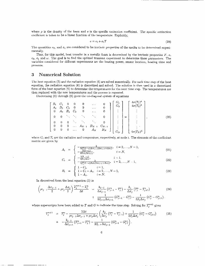
where p is the density of the foam and e is the specific extinction coefficient. The specific extinction coeiiicient is t&en io be a liiieai fuiictiwn of the temperature. Expiicitiy,

e = eo + elT (19)

The quantities eo, and el are considered to be intrinsic properties of the media to be determined experi- mentally.

Thus, for this model, heat transfer in a metallic foam is determined by the intrinsic properties F , a, eo, el and w. The goal is to find the optimal transient experiment to determine these parameters. The variables considered for different experiments are the heating power, sensor location, heating time and pressure.

3 Numerical Solution The heat equation (5) and the radiation equation (6) are solved numerically. For each time step of the heat equation, the radiation equation (6) is discretized and solved. The solution is then used in a. discretized form of the heat equation ( 5 ) to determine the temperatures for the next time step. The temperatures are then replaced with the new temperatures and the process is repeated.

Discretizing (6) through (8) gives the tri-diagonal system of equations

B1 C1 0 0 0 . . . 0 A2 B2 C2 0 0 . . . 0 0 A3 B3 C3 0 . . . 0

0 0 ‘ . . ... . . . 0

0 0 0 ’ . . . . 0 0 0 0 . . . AN-^ B N - ~ C,-l 0 0 0 . . . 0 AN BN

where Gi and T, are the radiation and temperature, respectively, at node i. The elements of the coefficient matrix are given by

1 - c,, i = 1, l -Ci -Ai , i = 2 , . . . , N-1 , 1 - Ai, i, = N.

Bi =

In discretized form the heat equation ( 5 ) is

where superscripts have been added to T and G to indicate the time step. Solving for T;+l gives

6

The material properties of the metallic foam, pc, k, and 8, are all functions of temperature given by either poiynomiai approximations or interpolated from tabiil&ed data. The temperature used for ca = pacar k,, or ,& is the average temperature of the two endpoints of the interval Axa. Explicitly for < = <(T)

4 Simulated Experiments In this section the simulated experiment for determining the thermal properties of the metallic foam is described. The simulated experiment consists of heating the (one-dimensional) sample of nickel foam, at some pressure, for a particular time period with a heater of a specified power, while taking temperature measurements at one location in the body. Thus the variables of the experiment are the heater power, the sensor location, the pressure, the heating time, and the total duration of the experiment.

Increasing the power to the heater increased the ability to determine the material properties. Since there would be physical limitations on the heater power supplied, rather than using the power of the heater as a variable between different experiments, an approximation of a heating apparatus used by DaryabeigiI4 was made. This apparatus consisted of 2500 W cylindrical heating elements spaced 1.27 cm apart. This corresponds to about 310 MW/m2 and an effective thickness of b = .00098 m. The heater and the sample were placed 5.08 cm apart. A cold plate, kept at room temperature, is considered to be along the other side of the sample.

The temperature of the heater, node one in the discretized form of the heat equation, is determined from a lumped mass model. Under this model the heater must satisfy the differential equation

where = 2600 kg/m3 is the density of the heater and ch = 800 J/(kg K) is the specific heat of the heater. The power supplied to the heater is qan=31O MW/m2 when the lieater is powered and zero otherwise, while qorrl is the heat loss to the sample and the surroundings.

The losses from the heater include radiative transfer to the surroundings and to the sample. The radiative heat losses are given by

where Eh = .05 is the emittance of a water-cooled mirrored surface behind the heater, TO is the mirror temperature (300.6 K), and T, is the temperature of the surface of the sample. Gas conduction from the heater to the sample is also included, described by

The total heat flow out of the heater is qozrl = q&,t + q&t. A typical experiment starts at room temperature, then the heater is powered for a period of time while

sampling the temperature at a particular location. Sampling continues for an additional period after the heater power is off. The heater model is incorporated into the transient finite difference code after the temperatures for each time step are found.

5 Optimality Criterion The goal of this study is to examine a wide range of simulated experiments and determine the best experiment for determining the properties of the metallic foam. The suitability of individual experiments is determined from the sensitivity of the temperature with respect to the sought-after thermal properties of the sample, F , a, eo, el and w. Relabelling the parameters b k , IC = 1,. . . , 5 , the normalized sensitivity coefficient for the kth parameter, at the i th time step, is defined as

7

Perturbing the parameters by a small amount, (1 + 6 ) b k , the sensitivity coefficients can be approximated by

The value of 6 = ,0001 was found to give well-behaved values for X . In general an experiment is better if the sensitivity coefficients are larger. In addition, for experiments

with more than one parameter the sensitivity coefficients must be linearly independent. For these reasons the optimality criterion used is

The sensitivity matrix, X, is defined by

where T is a vector of the temperatures at each sampling time. In (32), D is normalized by the maximum temperature, T,,,, squared and the number of sample temperatures, n, all taken to the power p (the number of parameters) in order to obtain a fair comparison among different experiment^.^

The sensitivities are partial derivatives at a particular value of each parameter. The parameter values used for this study are given in Table 1, as reported by Su1lins.l’ For all of the examples the thickness of nickel foam was 13.6 mm.

Table 1: Parameter values for simulated experiments

6 Optimal Experiment Design Our experience with thermal conductivity measurements, with no radiation present, suggested that it is best to heat the sample as rapidly as possible for a period of time while taking measurements a t the surface closest to the heater. This is also the best approach for radiation/conduction materials. A variety of simulated experiments were explored by varying the pressure, the duration of the heating and the total duration of the experiment. Initially the simulated experiments were terminated at the time corresponding to the peak value of the optimality criterion, D. It was found, however, that extending the experiment duration increased the accuracy of the parameter estimation. For experiments at lower pressures radiative heat transfer is more dominant, while at higher pressures heat transfer due to conduction is more significant. It was thus expected that the optimum case would occur at moderate pressures since three of the parameters are related to radiation and two are related to conduction.

The approximate conditions for the optimum experiment were found first by trial and error to find a rough value of the maximum of D , after which an optimization routine was run with the rough value as the initial guess. The maximum value of D found was 3.383-16. This value resulted from an experiment conducted at 0.190 mm Hg in which the heater WZLS run for 269 seconds and the temperature wils sampled every 10 seconds for a total duration of 840 seconds. In Figure 1 the optimality criteria is graphed versus time for a few simulated experiments in which the optimum heating time was used and the pressure was varied around the optimal pressure. In Figure 2, D is graphed versus time with the pressure fixed at 0.19 mm Hg for various heating times. As can be seen from the figure, the exact heating duration is not too critical. For heating times between 260 and 290 seconds the maximum value of D only varies by about four percent. In general if the sample is continuously heated the D value rises to a maximum and then begin to

8

decrease as the system reaches steady state. If instead the heater is shut off, at some time, the the value of D dramatically increases until the system again :ears steady state (room tempcrature). The rise in the D values when the heater is shut off is so dramatic that in most cases it is impossible to see the rise in the D values during heating if the entire experiment is graphed on the same scale. In Figure 3 the same curves given in Figure 2 are repeated along with a curve corresponding to constant heating for 1200 seconds. The separation in the four curves prior to the heater being shut off is due to each experiment reaching a different maximum temperature which is included in the normalization. The best time for heating (269 seconds) appears to be near the location where the D curve changes from concave up to concave down. In Table 2 the maximum value of D obtained for various pressures and heating times is summarized.

Table 2: Maximum D values for experiments

p [mmHgl Heating Duration [sec] 250 260 269 280 290 300

0.09 1.303-16 1.30E16 1.303-16 1.30E16 1.283-16 1.273.16 0.14 2.693-16 2.713-16 2.723-16 2.713-16 2.693-16 2.673-16 0.19 3.193-16 3.233-16 3.383-16 3.253-16 3.243-16 3.223-16

0.29 4.73E16 4.51E-16 4.323-16 4.153-16 4.01E16 3.893-16

It should be noted that for the optimal experiment one would want to stop taking data as soon as D reached its maximum value. From Figure 1 or Figure 2 this is at 840 seconds. This time is also not too critical, since for any value between 830 seconds and 900 seconds D will still be within one percent of its maximum value. Thus for this model the optimal experiment for determining the material properties is for the sample to be heated for 270 seconds at a pressure of 0.19 mm Hg with sampling every 10 seconds until 840 seconds have elapsed.

In Figure 4 the heat flux for the optimal experiment is given as a function of time. The total heat flux is approximately a step function while the radiative heat flux and heat flux due to conduction are of the same order, as expected. The temperature profile for the optimal experiment is given in Figure 5 . One can see from the temperature profile the system has not reached steady state when the heater is shut off.

0.24 4.323-16 4.113-16 3.933-16 3.783-16 3.653-16 3.533-16

7 Estimation of Parameters In this section the parameters are determined using three simulated experiments. Experiment 1 is the experiment found using the optimality criterion in the previous section. Experiment 2 is the same as experiment 1 except da.ta is taken for 2000 seconds. Experiment 3 consists of two heating events concate- nated into one simulated experiment, where one of the heating events is dominated by conduction flux and the other is dominated by radiative flux. Data for all of the simulated experiments are obtained by calculating the exact temperatures using the values of the parameters given in Table 1 and then corrupt- ing them with random noise with a standard deviation of 0.08 K. The standard deviation was chosen to correspond with the maximum standard deviations reported by Sullins” for actual experiments in the same temperature ranges. A nonlinear Levnberg-Marquardt parameter estimation routine is used t o fit the model parameters.15

For simulated experiment 1 the optimum experiment determined in the previous section was used. It consists of running the heater for 269 seconds and taking measurements until 840 seconds elapsed. The gas pressure is 0.19 mm Hg. The residuals between the exact and perturbed (noise added) temperatures, Tpert - Tezact., and between the exact temperatures and those calculated using the estimated parameters, TCst-TezncL, are given in Figure 6. The residuals between the exact temperatures and those calculated with the estimated parameters is less than 0.5 K and is biased towards overestimating the exact temperatures. In addition the error in the calculated temperatures exceeds the random noise added to the exact values. The estimated vdues of the psrameters along wit,h their 90% confidence intervals are given in Table 3.

Since at 840 seconds the temperature was still significantly above room temperature, for simulated

9

Table 3: Parameter values for simulated experiment 1

eo el W F a Exact 9.8503+00 -2.6303-03 9.930E01 6.850E-03 3.890E+02

Estimated 9.838Ef00 -2.6193-03 9.930E01 6.5823-03 4.696E-tO2 Percent Error -0.127 -4.17E01 4.383-03 -3.91E00 2.07E01

90 % Confidence Interval 6.5513-03 4.9223-06 3.152E05 7.9563-05 2.821E+01

experiment 2 the same heating time was used, but the temperature sampling was extended to 2000 seconds. By 2000 seconds the temperature at the sensor had cooled to 305 K. The results were much better both in terms of the residuals (See Figure 7) and the parameter estimation (see Table 4). The errors in the temperatures were less than .05 K while the parameters were found accurately within about one percent.

Table 4: Parameter values for simulated experiment 2

eo el W F a Exact 9.850Ef00 -2.630E03 9.930E-01 6.8503-03 3.8903+02

Estimated 9.853Ef00 -2.6333-03 9.9303-01 6.8743-03 3.8193+02 Percent Error 3.4893-02 1.2253-01 -1.2333-04 3.5213-01 -1.824E+OO

DO % Confidence Interval 6.569E03 4.9253-06 3.191E05 5.1183-05 1.529Et01

Table 4 shows that simulated experiment 2 estimated all of the parameters accurately, except for the coupling coefficient, a. Various other experiments with single heating events were tried, without success, in order t,o find the coupling coefficient more accurately. The coupling coefficient is only significant when the conduction through the gas is significant. This means a will be more important in experiments conducted at high pressure. In addition it should be easier to determine a from an experiment in which the radiative heat transfer is less important. Based on this information, simulated experiment 3 was constructed from a pair of heating events: one that was optimal for determining the conduction parameters; and one that was optimal for finding the radiation parameters. Noise was added to the data from this pair of heating events. The data sets were then concatenated as one data set for the parameter estimation. It should be noted that although optimal heating events were found for both the conduction and radiation parameters with the other parameters fixed, for the analysis of the concatenated data, all of the parameters were considered to be unknown.

For the conduction-optimal heating event, increasing pressure was found to improve the estimation of a and F. However, an increase in pressure from 1 to 10 atmospheres increased the D values by less than one percent. Since it woiild be much easier to obtain a pressure of one atmosphere this was used for the conduction-optimum heating event. In this case, it was also found that using more power i n the heater was better. Therefore the only variables to determine was how long to power the heater and how long t,o sample the temperature. From Figure 4 it can be seen that the flux due to conduction reaches a peak at about 20 seconds. At one atmosphere this peak moves to about 23.6 seconds, which was used for the conduction-optimal heating event. The temperature was sampled every second instead of every ten seconds. It was found that a data duration of 150 seconds provided good estimation of conduction parameters. Strict use of the D parameter would have resulted in a shorter experiment, but as with the single heating event the sample had not cooled very close to steady state by that time.

For the radiation-optimal heating event, D is the largest for a vacuum (no gas conduction). Sullins" reported using a minimum pressure of 0.0001 mm Hg so this value was chosen as a practically obtainable minimum pressure. For the experiments discussed so far, the initial heating had a significant conduction flux (see Figure 4). In Figure 8, the ratio of the conduction heat flux to the radiation heat flux is plotted for a few different heating times. It can be seen from the figure that if the sample is heated for 30 seconds this ratio is neai:y zeiO hi a !age portion of the cxpcrirnent. T!:is corresponds to the experizent being dominated by radiation. For this reason the radiation-optimal experiment was to heat the sample for 30

10

seconds and then data was sampled for 100 seconds. Again a longer sampling time was used than the D value indicated was optirrium.

Simulated experiment 3 consisted of the conduction-optimal and radiation-optimal heating events com- bined together. The residuals for simulated experiment 3 are given in Figure 9. The estimated parameters a.nd their 90% confidence intervals are given in Table 5. As can be seen in the figure and the table, the temperatures and the parameters are estimated accurately.

Table 5 : Parameter values for combined conduction and radiation experiments

eo el w F a Exact 9.8503+00 -2.6303-03 9.9303-01 6.8503-03 3.8903+02

Estimated 9.8443+00 2.6263-03 9.9303-01 6.8383-03 3.9053+02 Percent Error 6.2713-02 1.6663-01 -2.6963-05 1.7923-01 -3.9603-01

90 % Confidence Interval 1.9443-02 1.6683-05 2.8183-05 9.1073-06 8.7713-01

The sensitivity coefficients (normalized by their maximum value) are plotted for simulated experiment 1 in Figure 10. The sensitivity for a has nearly the same shape as the sensitivity for F . This indicates the sensitivities are almost linearly independent and is probably the reason it is hard to determine the value for a. A different choice of conduction parameters could probably be found that could be determined more accurately from simulated or actual experiments.

Simulated experiment 3 provides more accurate results than either experiment 1 or experiment 2. For all the experiments, the strict use of the normalization of D by the number of samples taken tended to end the experiments before all useful data was taken. Unnormalized values of X T X values would indicate the sample should be heated to steady-state and then cooled back to room temperature, which would require a very long experiment. The best data duration appears to be somewhere between the duration determined by strict use of the maximum value of the normalized and unnormalized values of X T X .

8 Conclusion For future use of high porosity materials in thermal protection systems for reusable launch vehicles, their performance needs to be chahacterized over a wide range of temperatures and pressures. The goal of t,his research is to develop general-purpose protocols for designing transient experiments to measure ther- mal properties of high porosity materials. As a first step, a metal foam material was studied with an experimentally validated thermal model.

The D optimality criterion and consideration of the heat fluxes can lead to suitable experiments for determining the properties. Maximization of the optimality criterion D lead to an experiment containing one heating event that could be used to determine the radiation and conduction parameters. Strict use of the D parameter leads to experiments that were too short in the sense that more accurate parameter estimates could be obtained from simulated data sets of longer duration. By considering the model itself and in particular its conduction and radiation behavior, a set of two shorter heating events were found that provided more accurate parameter estimates.

The radiation parameter w was easily found to a high degree of accuracy by all of the experiments. The coupling coefficient, a , was the hardest parameter to determine. The sensitivity of the of the coupling coefficient and the sensitivity of the solid conduction efficiency, F , are similar in shape which indicates they are close to linearly dependent. The coupling coefficient was an ad-hoc parameter added to Sullins’ model in order to obtain agreement with experimental data at high pressures. This suggests that there may be a different pair of conduction parameters that could adequately model the conduction process and provide more robust estimation than exhibited here.

Acknowledgement This work was supported by NASA-Langley grant NAG-1-01087 under the supervision of Max Blosser.

11

Appendix The temperature dependent properties for nitrogen are from Daryabeigi.l2

8.1 Temperature Dependent Nitrogen Properties

ps = -1.7343 - 4 + 342.2161T (34) (35) (36) (37)

cs kg Pr

= = =

1.083.545 - 0.328T + 6.949E - 4T2 - 2.823 - 7T3 2.048E - 3 + 8.7513 - 5T - 2.4623 - 8T2 0.854 - 7.0853 - 4T + 9.008E - 7T2 - 3.2073 - 10T3

References

Dorsey, J. T. et al., “Metallic Thermal Protection System Technology Development: Concepts, Re- quirements and Assessment Overview”, Proceedings, 40th Aerospace Sciences Meeting, Jan 14-17, 2002, Reno, Nevada, paper AIAA 2002-0502.

Beck, J. V. and Arnold, K. J., Parameter Estimation, 1977, Wiley, NY.

Taktak, R., Beck, J. V., and Scott, E. P., “Optimal experimental design for estimating thermal prop- erties of composite materials,” International Journal of Heat and Mass Transfer, Vol. 36, No. 12, 1993, pp. 2977-2986.

Dowding, K. J. and Blackwell, B. F., ‘Sensitivity Amalysis for Nonlinear Heat Conduction,” Journal Heat Dansfer, 123, 1-10 (2001).

Cole, K. D., “Thermal Characterization of Functionally Graded Materials-Design of Optimal Exper- iments,” 8th Joint AIAA/ASME Thennophysics and Heat Transfer Conference, St. Louis, MO, June 24-27, 2002, paper AIAA 20002-2882.

Cole, K. D., “Analysis of Photothermal Characterization of Layered Materials-Design of Optimal Ex- periments,” 15th Symposium on Thermophysical Properties, Boulder, CO, June 22-27, 2003.

Daryabeigi, K., “Heat Transfer in High-Temperature Fibrous Insulation,” AIAA J. Thermophysics and Heat Tramfer, vol. 17, no. 1, 2003, pp. 10-20.

* Bhattacharyya, R., “Heat Transfer Model for Fibrous Insulations,” Thermal Insulation Performance, D. L. McElroy and R. P Tye, editors, American Society for Testing and Materials Technical Publication 718, Philadelphia, pp. 272-286, (1980).

Yuen, W. W., Takara, E., and Cunnington, G., “Combined Conductive/Radiative Heat Transfer in High Porosity Fibrous Insulation Materials: Theory and Experiment,” Proceedings, 6th ASME-JSME Joint Thermal En,,gineerin,g Conference, March 16-20, 2003, paper TED-AJ03-126.

’” Zhu H., et. al “Minumum Mass Design of Insulation Made from Functionally Gra.ded Design”, Proceed- ings, 43rd AIAA Structures, Structural Dynamics, and Materials Conference, Denver CO, April 22-25, 2002, paper AIAA-2002-1425.

l1 Sullins, A. D., and Daryabeigi, K. , “Effective Thermal Conductivity of High Porosity Open Cell Nickel Foam, ” Proceeding of the 35th AIAA Thennophysics Conference, Anaheim CA, June 11-14, 2001, paper AIAA 2001-2819.

l2 Daryabeigi, K., Desi,gn of High Temperature Multilayer Insulation for Reusable Launch Vehicles, Ph.D. dissertation, University of Virginia, May 2000.

12

l3 Rohsenow, W. M., Hartnett, J.P., and Cho, Y.I., Handbook of Heat Transfer, Sd Edition, The McGraw-

l4 Daryabeigi, K., Knutson, J. R., and Sikora, J. G., “Thermal Vacuum Facility for Testing Thermal

l5 Press, W. H., Numerical Recipes in FORTRAN 77, Cambridge University Press, New York, 1996.

Kl l Companies, Inc., 1398.

Protection Systems,” NASA TM-2002-211734, June 2002.

I 3.50E-16 1

3.00E-16

2.50E-16

A 2.00E-16 Y

1.50E-16

1.00E-16

5.00E-17

O.OOE+OO 0 200 400 600 800 1000 1200

Time (sec)

Figure 1: D for 269 seconds of heating at various pressures in mm Hg

13

3.OE-16

2.5E-16 n Y - 2.OE-16 n

1.5E-16

1.OE-16

5.OE-17

O.OE+OO

0 200 400 600 800 1000 1200

Time (sec)

Figure 2: D for P=O.19 mm Hg and various heating times

1 .OE-17

9.OE-18

8.OE-18

7.OE-18

6.OE-18 n

5.OE-18 P

4.OE-18

3.OE-18

2.OE-18

I .OE-18

O.OE+OO 0 50 100 150 200 250 300 350 400 450 500

Time (sec)

Figure 3: D for P=O.19 mm Hg during heating.

14

6000

5000

4000

3000

2000

1000

0

-1 000

1100

1000

900

800

700

600

500

400

300

I

0 100 200 300 400 500 600 700 800

Time (sec)

Figure 4: Heat fluxes for P=O.19 mm Hg and 280 seconds of heating.

0 200 400 600 800 1000 1200

Time (sec)

Figure 5: Temperature for P=0.2 mm Hg and 280 seconds of heating.

15

0.6

0.4

- 0.2 Y In m - 3 0.0 - E In 9)

-0.2

-0.4

-0.6

i j

i

[ Tpert -Test 1 i

i j j

i

0 100 200 300 400 500 600 700 800

Time (sec)

Figure 6: Temperature residuals for simulated experiment 1

A

. . ... __ - . -. .. . .. 0.25 -

0.2 I

0.15

0.1

3 0.05 3

In W

E o

e -0.05

-0.1

-0.15

-0.2

-0.25

*- * * **

0 500 1000 1500 2000

Time (sec)

Figure 7: Tcmperature residuals for simulated expcriment 2

16

5.0 I n

0.2

4.0 3.0 ~

A

gs U 2.0

1

-1 .o 0 50 100 150 200

Time (sec)

Figure 8: Ratio of conduction to radiation flux for different heating times in seconds.

0.15

0.1

0.05 h

ln - Y o E 3 -0.05 a!

-0.1

-0.15

-0.2

-0.25

* * * * 6

* * ** -4 1 Tpert -Tcalc]

0 50 100 150 200 250

Time (sec)

Figure 9: Temperature residuals for simulated experiment 3.

17

1 .o

0.8

0.6 In al .= 0.4 > In 0.2

0.0

-0.2

E -0.4 z

.-

.- C .- S

'z1 a, N

m

-0.6

-0.8

-1 .o

I / I

0 200 400 600 800 1000 1200 Time (sec)

Figure 10: Sensitivities for conduction portion of simulated experiment 3

18