Optimal Fertilizer Warehousing and Distribution Systems for Farm Supply Cooperatives

Phil Kenkel Department of Agricultural Economics

Oklahoma State University

Fredy Kilima Department of Agricultural Economics

Oklahoma State University

Paper Presented at NCR-194 Research on Cooperatives Annual Meeting

November 2-3, 2004 Kansas City, Missouri

Optimal Fertilizer Warehousing and Distribution Systems for Farm Supply Cooperatives

Phil Kenkel Professor and Bill Fitzwater Cooperative Chair 516 Ag Hall Department of Agricultural Economics Oklahoma State University Stillwater Oklahoma 74078 405-744-9818 kenkel@okstate.edu (contact author) Fredy Kilima Department of Agricultural Economics 421-B Ag Halll Oklahoma State University Stillwater Oklahoma 74078 lukeheya@hotmail.com

2

Optimal Fertilizer and Warehousing and Distribution Systems

for Farm Supply Cooperatives

Introduction

Fertilizer sales and application services are important business areas for farm

supply cooperatives. These firms account for roughly one-third of the $800M, which

U.S. producers paid for fertilizer, lime and soil amendments in 2003 (USDA, 2004).

Many cooperatives are re-examining the structure and organization of their fertilizer

operations. A number of forces are impacting the retail fertilizer industry. Differential

production costs have shifted the production of nitrogen-based fertilizer away from

domestic manufacturers to off shore suppliers. The portion of nitrogen fertilizer imported

into the U.S. grew from 21% in 1999 to 42% in 2002 (U.S. Geological Survey).

The production shift has impacted the form of nitrogen fertilizers. Historically,

anhydrous ammonia has been the least cost form of nitrogen fertilizer. Because the

infrastructure to off-load anhydrous ammonia and transport it to demand regions is

limited, the shift toward off-shore supply sources has led to a shift to urea and other dry

forms of nitrogen fertilizer (Agriliance). Changing farm demographics have also

contributed to the shift to dry fertilizer forms. Large-scale producers typically find it

more economical for the input supplier to apply fertilizer using large-scale machinery.

Most agribusinesses offering custom fertilizer application concentrate on dry and liquid

(UAN) forms of nitrogen fertilizers. Security concerns associated with theft of

anhydrous ammonia for use in the illegal drug manufacturing has also contributed to the

shift to dry formulations.

3

Another factor impacting the structure of cooperative fertilizer operations has

been the consolidation among local cooperatives. A USDA study identified 367 mergers

and consolidations among grain cooperatives during the 1993 to1997 time period

(USDA, 1998). As local cooperatives consolidate and expand their geographic trade

territories they often attempt to consolidate their existing systems of multiple warehouses.

Determining the feasibility of a centralized warehouse system is complex. Centralization

generally reduces warehousing costs since construction and operating costs decrease with

size. However centralization increases the warehouse-to-field transportation costs. Shifts

in fertilizer product forms further increases the complexity of analyzing warehousing

centralization as per-unit warehousing and transportation costs differ dramatically across

anhydrous, dry and liquid formulations.

This study pursues two objectives related to fertilizer warehousing and

application: (1) Identify the major cost components of a typical fertilizer warehousing

and distribution system and product margins and fees needed to cover costs; (2)

Determine the optimal level of warehouse centralization and equipment complement.

Analytical Model

The analytical model for this study is a capacitated discrete mixed integer-

programming (CDMIP) model. Conceptually, the model is classified as capacitated

because upper limits were imposed on warehouse storage and machinery capacities. The

model is discrete because demand locations as well as flow of materials and equipment

between origin-destination pairs were specified. The model is structured in a mixed

integer-programming (MIP) framework because the structure accommodates discrete and

4

continuous variables to determine optimal location and size of a facility (Tembo). The

MIP also uses fixed charges that are amortized over the economic life of facilities and it

allows planners to assess opportunity costs for funds (Faminow). In general, MIP has

been extensively used to solve plant location and machinery selection problems (e.g.

Köksalan, Süral, and Kirca; Camarena, Gracia, and Sixto; Ghassam et al.; and Saadoun).

The CDMIP model selects the warehouse configuration and application fleet that

minimize transportation, warehousing, machinery and application costs subject to supply,

demand, facility and equipment capacity constraints. This cost minimization approach is

adopted because in supply chains the consolidation of materials in warehouses and

coordinated use of business assets has emerged as an effective cost-saving method due to

high percentage of total distribution or costs associated with transportation and fixed-

asset charges (Chiang and Russell; Herer, Tzur, and Yücesan; Mason et al.).

In the fertilizer industry, the supply chain entails transportation of fertilizers from

manufacturers or importers to storage facilities and finally to producers in known service

regions. In addition to fertilizer distribution, most of the retailers also own fertilizer

applicators that are rented to individual producers and other firms. Thus, a significant

cost reduction in the fertilizer supply chain could be achieved through efficiency that

might be apparent in coordinated transportation, warehousing, and application.

Therefore, a cost minimization model was developed to represent a total coordination of

business activities because improving efficiency is a goal that cannot be pursued in

isolation. A conceptual model for the cost minimization problem is discussed next.

5

In brief, for a given fixed-cost F j and a capacity constraint λ j of the jth facility,

the cost minimization function Z for the ith activity linked to the jth facility, with a

variable cost Cij and activity level Qij is mathematically given as:

(1) ,Min ,

YFQCZ jj

jiji j

ijYQ jij

∑+∑∑=

Subject to: (2) jDQ j

iij ∀≥∑ (demand constraint)

(3) iSQ ij

ij ∀≤∑ (supply constraint)

(4) { } njYYQ jjji

ij ..., ,2 ,1 ,1 ,0 , =∀∈≤∑ λ (capacity constraint)

(5) 0≥Qij (non-negativity condition)

This problem set-up ensures that a cost Cij is incurred only if a facility Y j is

acquired. In the CDMIP model D j and Si are aggregate demand and supply,

respectively. Equations 1 through 5 are the basic components of an empirical model used

in this study. The empirical model was developed following the CDMIP model specified

above. The objective function for the empirical model is given as:

(6) XX

XXXZ

aii a

awii w

w

afii a f

afiwfii j w f

wfiswii s w

swi

∑ ∑+∑ ∑+

∑ ∑ ∑+∑ ∑ ∑ ∑+∑ ∑ ∑=

= == =

= = == = = == = =

3

1

7

1

3

1

3

1

3

1

7

1

14

1

4

1

2

1

7

1

14

1

4

1

4

1

7

1

Min

ββ

βββ

The objective function is minimized subject to the following constraints:

(7) 4 2,..., 1, 4

1

7

1=∀≤∑ ∑

= =sSUPX si

i wswi (fertilizer supply constraint)

(8) 14 ..., ,2 ,1 4

1

7

1=∀≥∑ ∑

= =fDEMX fi

i wwfi (demand constraint)

(9) { }

321;721

,10 3

1

4

1

,, i , ..., , w

, X, XψX wiwiwi s

swi

=∀=∀

∈≤∑ ∑= = (warehouse storage constraint)

(10) 1,2,3 3

1

14

1=∀≤∑ ∑

= =aXX aia

i fafi λ (applicator capacity constraint)

6

(11) ∑∑ =∀≤∑ ∑= == =

4

1

4

1

4

1

14

17 ..., ,2 ,1

i sswi

i fwfi wXX (fertilizer flow requirement)

(12) { }

321721210

,, i; , ..., , a , ..., n, , X ai

=∀=∀∈

(integer)

(13) 14 ,..., 2 ,1 3

1

7

1

3

1

7

1=∀∑ ∑=∑ ∑

= == =fXX

i wwfi

i aafi (application requirement)

(14) 0 , ≥ X,XX afiwfiswi (non-negativity condition)

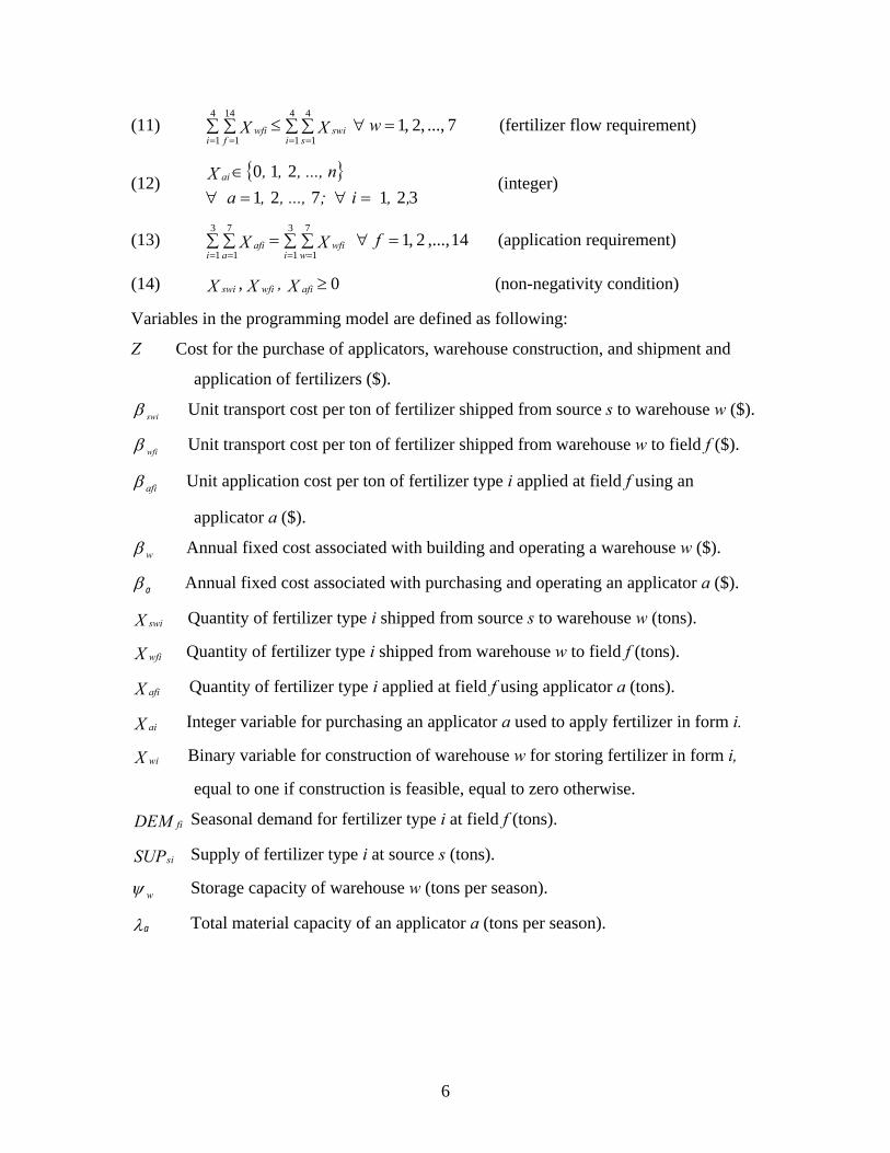
Variables in the programming model are defined as following:

Z Cost for the purchase of applicators, warehouse construction, and shipment and

application of fertilizers ($).

β swi Unit transport cost per ton of fertilizer shipped from source s to warehouse w ($).

β wfi Unit transport cost per ton of fertilizer shipped from warehouse w to field f ($).

β afi Unit application cost per ton of fertilizer type i applied at field f using an

applicator a ($).

β w Annual fixed cost associated with building and operating a warehouse w ($).

β a Annual fixed cost associated with purchasing and operating an applicator a ($).

X swi Quantity of fertilizer type i shipped from source s to warehouse w (tons).

X wfi Quantity of fertilizer type i shipped from warehouse w to field f (tons).

X afi Quantity of fertilizer type i applied at field f using applicator a (tons).

X ai Integer variable for purchasing an applicator a used to apply fertilizer in form i.

X wi Binary variable for construction of warehouse w for storing fertilizer in form i,

equal to one if construction is feasible, equal to zero otherwise.

DEM fi Seasonal demand for fertilizer type i at field f (tons).

SUPsi Supply of fertilizer type i at source s (tons).

ψ w Storage capacity of warehouse w (tons per season).

λa Total material capacity of an applicator a (tons per season).

7

Four distinct models were specified and estimated in this study. The first model

represented the application of anhydrous ammonium and DAP in fall followed by a “top

dressing” application of UAN in spring. Anhydrous ammonium was assumed to be

farmer applied with the DAP and UAN applied via the fertilizer supplier’s large-scale

applicators. This model can be considered the base-line scenario and represents historical

application practices. The second model involved a combined fall application of DAP

and Urea followed by a spring “top dressing” application of UAN. This model represents

a likely response to the elimination of anhydrous ammonium. The third model involved

application of a blend of urea and DAP in the fall. The fourth model involved an

application of DAP in the fall followed by an application of UAN in the spring. This

model relates to the latest recommendations of Oklahoma State University agronomists.

The basic premise is that fall nitrogen applications based on expected average yield

potential are likely to either under estimate or over estimate the nitrogen needs in each

particular growing season. Producers are being encouraged to delay nitrogen applications

until spring and to make applications (either variable rate or constant rate) based on the

crop condition and potential. While the results of this study do not address the possible

savings due to variable rate application, they do provide useful information in describing

how the costs of warehousing, transportation, and application would be affected by a shift

to spring nitrogen application.

A common assumption in these models is that fertilizers were applied to provide a

total of 95 pounds of nitrogen and 25 pounds of P2O5 per acre. These models were

solved using the GAMS CPLEX algorithm. The program is useful for solving different

types of mathematical models such as linear and non-linear programming, relaxed mixed

8

integer programming, mixed integer programming, relaxed mixed integer non-linear

programming with discontinuous derivatives, and mixed integer nonlinear programming

with discontinuous derivatives.

Data

Data for the models were obtained from an Oklahoma grain and farm supply

cooperative that operates nine fertilizer warehouses in a five county trade territory. The

case study situation provided a realistic configuration of transportation distances between

warehouses and fertilizer supply sources, and between warehouse and field locations.

The cooperative also provided information on fertilizer sales by type, available

application days, hours of operation, shipment costs, and equipment road and field speed.

Warehouse and equipment costs and capacity information were obtained from equipment

manufactures and warehouse construction contractors. Additional data such as interest

and insurance rates, fuel price, and wage rates were obtained from secondary sources.

The primary and secondary data were used to approximate the variables specified in the

empirical model. Detailed information regarding the estimation procedures is provided

below.

Machinery Cost Estimation

Variable and fixed costs associated with the use and ownership of fertilizer

applicators were estimated following the American Society of Agricultural Engineers

(ASAE) machinery standards. This method was adopted because it uses standardized

cost coefficients based on many years of observed engineering estimates. The method

9

gives best estimates when all necessary information needed to estimate machinery costs

are not available (Dumler, Burtons, and Kastens).

Machinery Variable costs was calculated as a sum of fuel cost, oil and filter cost,

repair cost, labor cost, and machinery transfer cost. However, Machinery transfer cost to

and from field is not part of the ASAE specification. The intuition behind the inclusion

of this variable is that the proposed model allows machines located in one region to be

used in another region, thus incurring machinery transfer costs. Fixed costs include

depreciation, interest cost, and insurance expense. Property tax is typically considered a

fixed cost. However, it is not included in this model based on the assumption that there is

no property tax on farm machinery (Kastens). Conventionally, these costs are estimated

on a cost-per-acre basis and account for field capacity of machinery, which is normally

calculated using width and speed of machinery, adjusted for field efficiency. In this

study the costs-per-acre were converted into costs-per-ton by dividing all fixed and

variable costs by their respective fertilizer application rates measured in tons per acre.

Field capacity used to estimate various machinery costs was calculated following

the ASAE Agricultural Machinery Management Standard 5.1. Fuel cost was calculated

using after-tax price of diesel, and fuel consumption rates following the ASAE

Agricultural Machinery Management Standard 6.3.2.1. Oil and filter cost was estimated

using the ASAE Agricultural Machinery Management Standard 6.3.3 and was calculated

as 15 percent of fuel cost. Repair cost was calculated based on accumulated hours of use

following ASAE Agricultural Machinery Management Standard 6.3.1. Labor cost was

calculated using pre-tax wage rate including all payroll benefits and machinery labor

hours that are estimated based on field capacity of machinery (Cross). Applicator

10

transfer cost was calculated as a sum of fuel cost, oil cost, and repair and maintenance

cost that would be incurred if applicators were allowed to cross from their locations to

other service regions.

Annual cost of economic depreciation of machinery was calculated as the

difference between the dollar values of machine at the beginning of a farming year and

the value at the end of the year. Depreciation cost was estimated using ASAE Machinery

Management Standard 6.1. Interest cost was estimated following an approach

recommended by Cross using a 5 percent rate suggested by Langemeier and Taylor.

Insurance cost was also calculated following Cross’s approach and was estimated using

initial cost of machinery and insurance rate. Insurance rate used was 0.25 percent

consistent with the ASAE recommendations.

Estimation of Fertilizer Demand

Fertilizer demand was estimated based on the acreage applied by case-study

firm’s custom and company’s rigs in 2001/2002 wheat production year. Fertilizer

tonnage was calculated by multiplying the nitrogen and phosphorous application rates for

Oklahoma wheat, which are 95 pounds of N and 25 pounds of OP 52 per acre by historical

acreage data (USDA, 2003). However, to meet the specified wheat nutrients

requirement, there are many fertilizer application options for producers to choose from.

Therefore, producers may demand unique mixes of fertilizers based on personal

preferences. However, such unique demands can only be modeled if preferences are

known with certainty. Since preferences are not known it was necessary to choose

among choices a base line application system and supportive systems that might replace

11

it when it is shocked by demand or supply factors. The base line application system is

defined as an application system that represents historical practice.

Estimation of Seasonal Material Capacities of Fertilizer Applicators

The mathematical model was also structured to identify optimal numbers of each

type of fertilizer applicator. To facilitate this choice, it was necessary to determine a

maximum quantity of fertilizer each of the applicators could apply per season. This

variable was calculated using material capacity and effective daily working hours.

Material capacity was computed following the ASAE formula presented in Equation (15).

(15) 25.8

100. ⎟

⎠⎞

⎜⎝⎛⋅

=

EFyWSCm

where Cm is material capacity (ton per acre), y is application rate (ton per acre).

Effective daily working hours of a machine is defined as maximum number of hours a

machine can work in one day, and was calculated by adjusting potential daily working

hours ( )H d for machinery round trip travel time to and from field ( )H t , as well as

potential time wastage due to machinery breakdown, also known as machine failure or

down time.

Adjustment for breakdown probability followed ASAE formula for accumulated

down time and is a function of accumulated hours of use ( )u . The down time ( )Dt for

diesel-fueled machines was calculated as:

(16) uDt4173.10003234.0 ⋅=

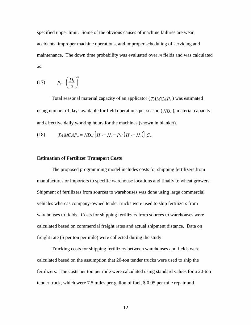
The breakdown probability ( )P b is formally defined as the probability of any

condition that prevents the operation of the machine or reduces its performance below a

12

specified upper limit. Some of the obvious causes of machine failures are wear,

accidents, improper machine operations, and improper scheduling of servicing and

maintenance. The down time probability was evaluated over m fields and was calculated

as:

(17) ⎟⎠⎞

⎜⎝⎛=

uDP t

m

b

Total seasonal material capacity of an applicator (TAMCAPa ) was estimated

using number of days available for field operations per season ( NDa ), material capacity,

and effective daily working hours for the machines (shown in blanket).

(18) ( )[ ] CHHPHHNDTAMCAP mtdbtdaa ⋅−⋅−−⋅=

Estimation of Fertilizer Transport Costs

The proposed programming model includes costs for shipping fertilizers from

manufactures or importers to specific warehouse locations and finally to wheat growers.

Shipment of fertilizers from sources to warehouses was done using large commercial

vehicles whereas company-owned tender trucks were used to ship fertilizers from

warehouses to fields. Costs for shipping fertilizers from sources to warehouses were

calculated based on commercial freight rates and actual shipment distance. Data on

freight rate ($ per ton per mile) were collected during the study.

Trucking costs for shipping fertilizers between warehouses and fields were

calculated based on the assumption that 20-ton tender trucks were used to ship the

fertilizers. The costs per ton per mile were calculated using standard values for a 20-ton

tender truck, which were 7.5 miles per gallon of fuel, $ 0.05 per mile repair and

13

maintenance cost, and $ 0.03 per mile tires cost (Dahl, Cobia, and Dooley).1 Therefore,

the tender truck cost per ton per mile was $ 0.27.

Estimation of Warehousing Costs and Storage Capacities

Data regarding warehouse construction costs and storage capacities were

collected when the study was conducted. Fixed costs included annual depreciation costs,

opportunity costs, maintenance costs, property values and insurance costs. Warehouse

annual depreciation costs were calculated using straight-line method expensed over a

period of 40 years, which is the life span of concrete/masonry buildings (South Carolina

State-Comptroller General’s Office). Other fixed costs were calculated as percentages of

warehouse construction value. Warehouse opportunity cost was estimated as 4% of the

value, maintenance as 3% of the value, and property value and insurance tax together as

2.5% of the value. Fixed cost for warehousing was calculated as a sum of all these costs

and was converted to cost per ton of fertilizer stored using storage capacities of the

warehouses.

Description of the Warehousing Structure

The structure of the analytical model also provided a basis for assessing

“economies of size” in fertilizer warehousing. To achieve this goal, two warehouse sizes

(big and small) for dry and UAN facilities were incorporated in the model. Big facilities

were five times the size of small facilities and were centrally located. The model

permitted construction of small warehouses at any location within the business area. The

1 The coefficients for repair and maintenance and tire costs were inflated from their year 1995 values. The inflation process was achieved through multiplying the ratio of year 2002 to year 1995 industry consumer price indices (CPIs) by the 1995 repair and maintenance value.

14

model did not require a central warehouse for anhydrous ammonia fertilizer because no

data on larger size facility was available. Costs for big facilities were $ 1.98/ton for dry,

and $ 2.27/ton for UAN. The costs per ton for small facilities were $ 5.67 for dry, $ 6.48

for UAN and $ 7.65 for anhydrous ammonia. In terms of storage cost, big facilities were

about 35% cheaper on a per ton basis.

Description of Application Equipment

Three different applicators, dry, liquid, and anhydrous were modeled in this study.

Dry applicators were used to apply DAP or a mix of DAP and urea. The working width

of dry applicators was 60 feet (Ft), and the field speed was 16.5 miles per hour (mph).

Liquid applicators were used to apply UAN, working width and field speed for these

applicators were 75 Ft and 19 mph, respectively. The dry and liquid applicators were

owned and operated by the case-study cooperatives. The working widths and field speed

specified above in conjunction with coefficients for self-propelled combine were used to

estimate costs for dry and liquid applicators.

With respect to anhydrous application, two types (big and small) applicators were

modeled. The working widths were 20 Ft for small, and 30 Ft for big applicators. The

field speed for both applicators was 5 mph, and their efficiency factor (EF) was 80.

These equipment were owned by the cooperatives and rented to wheat producers,

therefore, it was difficult to estimate variable costs associated with the use of farmer

operated applicators because farmer costs were not known. As a result, this study used $

5.82 per-acre anhydrous ammonia application cost suggested by Doye, Sahs, and Kletke.

Ownership costs for anhydrous applicators were estimated using secondary data.

Depreciation cost used was $ 1.94 per acre (Razarus and Selley). Insurance cost was

15

estimated using purchase price suggested by Langemier and Taylor and machinery hours

suggested by Harryman, Siemens, and Kirwan. Interest cost was approximated using

purchase price, machinery hours, and ASAE formula for computing remaining values of

field machine ( )RV as percent of purchase price at the end year n given in Equation (19)

below.

(19) )885.0(60 )(nRV ⋅=

Results and Discussion

In this study four alternative fertilization systems with the nitrogen component

involving fall anhydrous combined with a spring application of UAN, fall urea combined

with spring UAN, fall urea only, and spring UAN only were modeled. The first system

more closely reflects actual practices among Oklahoma’s wheat-growers. The second

system was adopted to assess the likely effects of eliminating anhydrous ammonia in the

supply chain following the overall decrease in domestic production and an increased role

of imported dry fertilizers. The third and fourth systems are not very common among

Oklahoma farmers and were included to analyze the extent to which combined costs of

satisfying nutrients demands could vary across different combinations of fertilizers. The

variation was useful in identifying a least-cost way of satisfying the demand. The

incorporation of the DAP and UAN combination in the analysis provided insights to the

feasibility of applying very little nitrogen in fall and supplementing the demand through

top dressed applications in spring which is advocated by agronomists (Gribble). Costs

for the modeled fertilization systems are summarized in Table 1. The cost for the

16

baseline-model excludes farmers’ cost of applying anhydrous ammonia. The estimated

costs are used to assess extents to which operating costs change from the baseline-case.

17

Table 1 Operating costs for different fertilizer application systems Costs ($)

Model

Fertilizer Transportation (From Sources to Warehouse)

Fertilizer Transportation (From Warehouses to Fields)

Fertilizer Application

Annual Warehousing

Applicator Ownership Total Cost

Base line-case (Model 1)

166,419.01

(0.79) 114,913.46 (0.55)

206,979.95 (0.99)

269,853.45

(1.29) 1,181,751.93

(5.63) 1,939,874.79

(9.24)

Model 2 282,592.85

(1.35) 138,894.11 (0.66)

206,979.94 (0.99)

302,128.83

(1.44) 1,171,352.06

(5.58) 2,101,947.80 (10.01)

Model 3 278,485.39

(1.33) 145,055.07

(0.69) 124,003.44

(0.59)

153,089.26

(0.73) 552,904.90

(2.63) 1,253,538.06 (5.97)

Model 4 324,880.19

(1.55) 226,105.48 (1.08)

206,979.95 (0.99)

334,528.83

(1.59) 1,171,352.06

(5.58) 2,263,846.51

(10.78)

( ) Represents per acre costs. Farmers apply anhydrous ammonia. When farmers’ cost was included, the application costs for the baseline-model was $

1,430,774.28 (6.82/acre) and the total cost was $ 3,163,712.12 (15.07/acre). Numbers does not add up exactly due to rounding. Source: GAMS output.

18

The model results provided interesting insights into costs of fertilizer warehousing

and application. The costs of transporting fertilizer from source to warehouse and

between the warehouse and fields accounted for almost 22% of the total system costs.

Warehouse ownership accounted for 14% and variable application costs were

approximately 10% of the total system costs. The largest cost components were the fixed

costs associated with applicator ownership, which were 54%. Cooperatives and other

agribusinesses recover fertilizer system costs through product margins and application

fees. Summaries of material and application costs are provided in Table 2.

19

Table 2 Material and Fertilizer Application Costs for the Modeled Systems Cost $

Model Description Material NH3 Application1 Fall Fertilizer Application2

Spring Fertilizer Application2 Total Cost

Baseline-case (Model 1)

23.66 5.82 3.00 3.00 35.47

Model 2 29.52 NA 3.00 3.00 35.52

Model 3 29.19 NA 3.00 32.19

Model 4 32.06 NA 3.00 3.00 38.06 Fertilizer prices used were $ 300 per ton of NH3, $ 256 per ton of DAP, $ 240 per ton of urea, and $ 165 per ton of UAN. 1 Represents estimated Farmers’ cost of applying NH3. 2 Represents estimated application fee charged by cooperatives.

20

The model results indicated that a product margin of $24/ton combined with a

$3.60/acre application fee was required to cover costs for the baseline-model. However,

results show that the product margin and application fees would need to increase to cover

costs for other models. The increases in product margins would be $ 5.86 for the second

model, $ 5.53 for the third model, and $ 8.40 for the fourth model whereas increases in

application fees would be $ 0.11 for the second, $ 0.14 for the third model, and $ 0.55 for

the forth model.

In summary model results presented in Tables 1 and 2 show that the cooperative’s

total transportation, warehousing and application cost did not vary substantially across

systems. While a shift away from anhydrous ammonia would obviously involve

transitional costs, the major impact would be the increase in material costs. However,

this impact need to be weighted against potential costs and advantages associated with

the timing of nitrogen application and opportunity costs associated with fertilizer applied

to crops that might be damaged by pests or bad weather.

The models were also structured to assess the feasibility of centralized

warehousing. Results indicated partial but not complete centralization of warehouses.

The feasibility of the observed centralization was evaluated through comparing costs

under partially centralized system with costs that would be incurred under non-

centralized storage and totally centralized storage.

In general, the models were constructed based on the assumption that

cooperatives would invest in new warehouse construction or analogously expansion of

storage capacities. However, the costs of existing warehouses were fixed and irrelevant

to the decision. Thus, direct comparisons of costs under partial centralized and non-

21

centralized warehousing would be misleading. To make results comparable only

transportation, application and equipment ownership costs were included in the

comparisons. The identified cost difference in transportation, application, and equipment

ownership could be considered by the agribusinesses and compared with the economies

of size in warehouse construction. Results for the comparisons are provided in Table 3.

22

Table 3 Comparison of transportation, application and equipment ownership costs for partially centralized and non-centralized business operations

Costs ($) Model Description Partial-Centralization Non-Centralized Base-line model 1,670,064.31

(7.96)

1,849,129.65 (8.81)

Model 2 1,799,818.97 (8.57)

2,136,563.19 (10.18)

Model 3 1,100,448.80 (5.24)

1,345,424.42 (6.41)

Model 4 1,929,317.68 (9.19)

2,311,713.82 (11.01)

Source: Own Computation.

23

Results indicated that partial centralization would decrease combined costs of

fertilizer transportation and application, and equipment ownership. The decreases were $

179,065.34 (0.85/acre) for the baseline-model, $ 336,744.22 (1.61/acre) for the second

model, $ 244,975.62 (1.17/acre) for the third model, and $ 382,396.14 (1.82/acre) for the

fourth model. The observed cost-savings were attributable to the benefits of economies

of size in warehousing and enhanced capacity utilization of the machines under partially

centralized arrangement.

Sensitivity evaluations were used to assess the feasibility of totally centralized

storage of fertilizers. The evaluation process was achieved through iterative reduction of

annual warehousing costs for the big facilities. These reductions reflected increased

economies of size for large warehouses. However, single warehousing never came into

the optimal solution. To illustrate the cost differential of a single warehouse, the models

were constrained to single large-scale dry and liquid warehouses. The cost disadvantage

of a central warehouse relative to the optimal solutions is provided in Table 4.

24

Table 4 The impact of single coordinated warehouse on operating cost Costs ($) Model

Change in Fertilizer Transportation (From Sources to Warehouse)

Change in Fertilizer Transportation (From Warehouses to Fields)

Change in Applicator Ownership Cost

Net Impact on Transportation and Application Cost

Model 2 -11,159.6 -(0.05)

+354,953.54 +(1.69)

+78,986.42 +(0.38)

+422,780.32

+(2.01)

Model 3 -6,035.24

-(0.03)

+321,600.83

+(1.53)

+78,986.41

+(0.38)

+394,552.00 +(1.88)

Model 4 -60,898.40

(0.29)

+472,432.41 +(2.25)

+157,972.83 +(0.75)

+569,506.84

+(2.71)

- Represents decrease in cost. + Represents increase in cost. The baseline-model is excluded from this analysis because data on large-scale storage of anhydrous ammonia was not available.

25

Results presented in Table 4 show that the adoption of a single coordinated

warehousing for dry and liquid fertilizers would increase operating costs and the number

of applicators. The increases in costs were $ 422,780.32 ($ 2.01/acre) for the second

model, $ 394,552.00 ($ 1.88/acre) for the third model, and $ 569,506.84 ($ 2.71/acre) for

the fourth model. These increases in costs offset the financial gains from economies of

size in warehousing, which are $ 239,760.00 ($1.14/acre) for the second model, $

113,400.00 ($ 0.54/acre) for the third model, and $ 272,160.00 ($ 1.30/acre) for the

fourth model.

In summary, this analysis indicates that in the supply and application of fertilizers,

fertilizer transportation and applicator ownership and fleet costs have much impact than

warehousing cost. These results suggest that cooperatives should carefully evaluate

warehouse-to-field transportation costs before consolidating warehouse locations.

Warehouse cost efficiencies were offset when fertilizer transportation cost increased and

machinery transportation time differences associated with centralization required the

purchase of additional applicators.

The empirical model was also used to examine how the optimal number of

applicators under the base-line model relates to current application equipment. This

comparison provided a qualitative assessment of efficiency of the case study

cooperative’s current compliment of application equipment. Results indicate that the

cooperatives would need seven dry applicators, ten liquid applicators, and fifty-three

anhydrous applicators. The current system has eight dry applicators, eight liquid

applicators and ninety anhydrous applicators. The least cost compliment of application

equipment was similar to the structure of case-study cooperative’s equipment suggesting

26

that the cooperative was operating its equipment near its engineered capacity. The

exception was anhydrous ammonia trailers. The number of trailers suggested by the

model was fewer than the number in use by the cooperative. This result validates

common complaints from cooperative managers on the inefficiencies in supplying

farmer-controlled equipment.

Summary and Conclusions

More recently, farm supply cooperatives in the U.S. have been striving to

coordinate businesses warehousing systems to keep pace with the changes in business

environment. The changes arise from growing global competition, increased regulations

in the industry for environmental and safety concerns, and changing demand. However,

as cooperatives attempt to consolidate warehousing activities they have to consider a

tradeoff between cost savings that arise from economies of size in warehousing and

increased warehouse-to-field fleet time and costs.

This study has developed mathematical models that are used to identify major

cost components of fertilizer warehousing, distribution, and application and

corresponding product margins and fees needed to cover costs for the studies

cooperatives. The models are also used to track the likely effects of eliminating

anhydrous ammonia in the supply chain as its production trend continues to decline, and

a shift from dry and anhydrous applications in fall towards spring applications of liquid

formulations. Additionally, the models also used to determine optimal level of

warehouse centralization and equipment complement. Scenario evaluation and

27

sensitivity analysis were incorporated in the models to assess the feasibility a single

location warehousing.

Results show that in fertilizer supply and application, fertilizer transportation and

applicator ownership costs have much impact than warehousing costs. Results show that

cooperatives would require product margins of $ 24, $ 30, $ 29, and $ 32 per ton and

application fees of $ 3.60, $ 3.71, $ 3.71, and $ 4.10 per acre for the baseline, second,

third, and fourth application systems, respectively. Overall, cooperative’s costs did not

vary substantially across the systems. Results suggest that the major impact of shifting

away from anhydrous ammonia would be the increase in producers’ material costs.

However, this impact need to be weighted against potential costs and advantages

associated with the timing of nitrogen application and opportunity costs associated with

fertilizer applied to crops that might be damaged by pests or bad weather.

Optimal solution indicated partial but not complete centralization of warehousing

and application activities. Costs under partial centralized system were lower than costs

under non-centralized and totally centralized system. Total centralization was infeasible

because increase in transportation costs outweighed gains from economies of size in

warehousing. Thus, cooperatives should carefully evaluate warehouse-to-field

transportation costs before consolidating warehouse locations.

The least cost compliment of application equipment was similar to the structure of

case-study cooperative’s equipment, which implies that the applicators are used near

engineered capacity. The exception was anhydrous ammonia trailers. The number of

trailers indicated in the model solution was fewer than the number in use by the

cooperative. This result validates common complaints from cooperative managers on the

28

inefficiencies in operating farmer-controlled equipment. Another reason for the high

number of anhydrous applicator is probably to accommodate peak demand, which might

arise due to unpredictable weather changes.

29

References

Agriliance “High Natural Gas Drives Ammonia Prices” Crop Nutrients Bulletin, Feb 11,

2003, http://www.agriliance.com/images/CropNutrientsbulletin.pdf.

Camarena, E. A., C. Gracia, and J. M. C. Sixto. “A Mixed Integer Programming Machinery Selection Model for Multifarm Systems.” Biosystems Engineering 87(2004): 145-154.

Chiang, W., and R. A. Russell. “Integrating purchasing and routing in propane gas

supply chain.” European Journal of Operational Research 154(2002): 710-729. Cross, T. “Machinery Cost Calculation Methods.” The University of Tennessee, Institute

of Agriculture, Agriculture Extension Service, AE&RD No. 13 E12-2015-00-032-98, 1998.

Dahl, L. B., D. W. Cobia, and F. J. Dooley. “Distribution Costs for Dry Fertilizer

Cooperatives.” Agricultural Economics Report No. 339, November 1995. Doye, D., R. Sahs, and D. Kletke. “Oklahoma Farm and Ranch Custom Rates, 2003-

2004.” Oklahoma Cooperative Extension Service, CR-205, 0404 Rev. Division of Agricultural Sciences and Natural Resources, Oklahoma State University.

Dumler, T. J., R. O. Burton, Jr., and T. L. Kastens. “Predicting Farm Tractor Values

through Alternative Depreciation Methods.” Review of Agricultural Economics 25(2003): 502-522.

Faminow, M. D. “The location of Fed Cattle Slaughtering and Processing: An

application of Mixed Integer Programming.” Ph.D. Dissertation, Department of Agricultural Economics, University of Illinois, Urbana, 1982.

Ghassam, A., A. K. Srivastava, T. H. Burkhardt, and J. D. Kelly. “Mixed-integer Linear

Programming (MILP) Machinery Selection Model for Navy bean Production Systems.” Transactions of the ASAE 29(1986): 81-89.

Harryman, W. R., J. C. Siemens, and B. Kirwan. “Machinery Cost Estimates: Field

Operations.” Farm Business Management handbook FBM-0101, University of Illinois, November, 1997.

Herer, Y. T., M Tzur, and E. Yücesan. “Transshipments: An Emerging Inventory

Recourse to Achieve Supply chain Leagility.” International Journal of Production Economics 80(2002): 201-212.

30

Kastens, T. “Farm Machinery Operation Cost Calculations.” MF-2244, Kansas State University Agricultural Experiment Station and Cooperative Extension Service, May 1997.

Köksalan, M., H. Süral, H., and Ö. Kirca. “A location-distribution application for a bear

company.” European Journal of Operational Research 80(1995): 16-24. Langemeir N. L., and R. K. Taylor. “A Look at Machinery Cost.” Kansas State

University Agricultural Experiment Station and Cooperative Extension Service, MF-842, 1998.

Lazarus, W. F., and R. A. Selley. “Farm Machinery Economic Cost Estimates for 2002.”

FO-6696, Department of Applied Economics, College of Agricultural, Food, and Environmental Sciences, University of Minnesota, September 2002.

Mason, J. S., P. M. Ribera, J. A. Farris, and R. G. Kirk. “Integrating warehousing and

transportation functions of the supply chain.” Transportation Research Part E 39(2003): 141-159.

Saadoun, T. “Agricultural Machinery selection and Scheduling of Farm Operations.”

PhD Thesis, University of Edinburgh, United Kingdom, 1989. South Carolina Comptroller General’s Office, “Useful Lives for Depreciation of Capital

Assets.” Unpublished Internet Resource available at web address: http://www.cg.state.sc.us/gasb34/training/segment2/handouts/AM1_Useful_Lives.pdf, State of Carolina, 2002.

Tembo, G. “Potential for Expansion of Wheat Processing Industry in Oklahoma.” MS

Thesis, Oklahoma State University, 1998. U.S. Geological Survey, Mineral Commodities Summaries, January 2004,

http://minerals.usgs.gov/minerals/pubs/mcs/. USDA, Rural Business-Cooperative Service (USDA/RB-CS). “Cooperative Historical

Statistics.” Cooperative Information Report 1, Section 26, April 1998. USDA, National Agricultural Statistics Services, Agricultural Statistics, 2003. USDA, National Agricultural Statistics Service “Farm Production Expense 2003

Summary.” July 2004.