Chapter 3 Optimal Filter Theory and Applications

References:

B.Widrow and S.D.Stearns, Adaptive Signal Processing, Prentice-Hall, 1985

S.M.Stearns and D.R.Hush Digital Signal Analysis, Prentice-Hall, 1990

P.M.Clarkson, Optimal and Adaptive Signal Processing, CRC Press, 1993

S.Haykin, Adaptive Filter Theory, Prentice-Hall, 2002

1

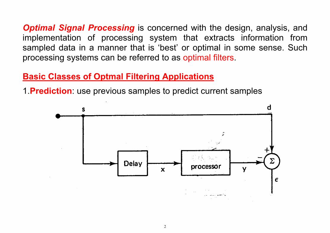
Optimal Signal Processing is concerned with the design, analysis, and implementation of processing system that extracts information from sampled data in a manner that is ‘best’ or optimal in some sense. Such processing systems can be referred to as optimal filters.

Basic Classes of Optmal Filtering Applications

1.Prediction: use previous samples to predict current samples

2

Speech Modeling using Linear Predictive Coding (LPC)

Since speech signals are highly correlated, a speech signal )(ns can be accurately modeled by a linear combination of its past samples:

)()(ˆ)(1

inswnsns iP

i−∑=≈

=

where }{ iw are known as the LPC coefficients. Techniques of optimal signal processing can be used to determine }{ iw in an optimal way.

2. Identification

3

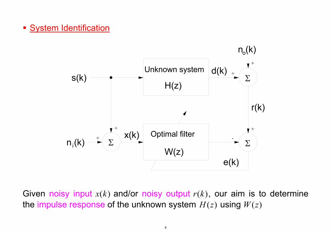
System Identification

Σ

ΣΣ

H(z)

Unknown system

Optimal filter

W(z)

+

++

+

+

-

s(k)

n (k)i

n (k)o

d(k)

r(k)

e(k)

x(k)

Given noisy input )(kx and/or noisy output )(kr , our aim is to determine the impulse response of the unknown system )(zH using )(zW

4

3. Inverse Filtering: find the inverse of the system

Signal Recovery

Given a noisy discrete-time signal:

)()()()( kwkhkskx +⊗=

where )(ks , )(kh and )(kw represent the signal of interest, unknown impulse response and noise, respectively. Optimal signal processing can be used to recover )(ks in an optimal way.

5

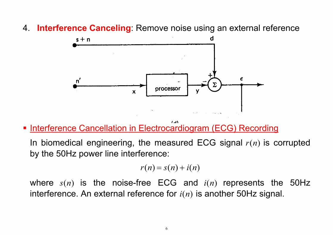
4. Interference Canceling: Remove noise using an external reference

Interference Cancellation in Electrocardiogram (ECG) Recording

In biomedical engineering, the measured ECG signal )(nr is corrupted by the 50Hz power line interference:

)()()( ninsnr +=

where )(ns is the noise-free ECG and represents the 50Hz interference. An external reference for )(ni is another 50Hz signal.

)(ni

6

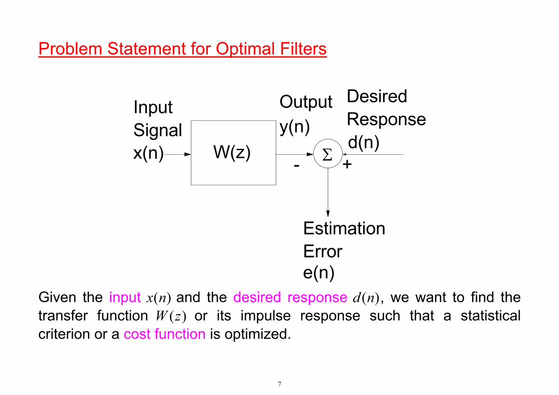
Problem Statement for Optimal Filters

W(z)x(n) Σ

y(n)d(n)

EstimationError

+-

InputSignal

Output

e(n)

DesiredResponse

Given the input and the desired response , we want to find the transfer function )

)(nx(

)(ndzW or its impulse response such that a statistical

criterion or a cost function is optimized.

7

Some common optimization criteria in the literature are: −1N

1.Least Squares : find )(zW that minimizes ∑=0

2 )(n

ne where N is the

number of samples available. This corresponds to least-squares filter design.

2.Minimum Mean Square Error : find )(zW that minimizes . This corresponds to Wiener filtering problem.

)}({ 2 neE

3.Least Absolute Sum : find )(zW that minimizes )(1

0ne

N

n∑−

=.

4.Minimum Mean Absolute Error : find )(zW that minimizes })({ neE .

5.Least Mean Fourth : find )(zW that minimizes . )}({ 4 neE

The first and second are two commonly used criteria because of their relatively small computation, ease of analysis and robust performance. In later sections it is shown that both viewpoints give rise to similar mathematical expression for )(zW .

Q.: An absolute optimization criterion does not exist? Why?

8

Least Squares Filtering For simplicity, we assume )(zW is a causal FIR filter of length so that L

∑=−

=

−1

0)(

L

i

ii zwzW (3.1)

The error function is thus given by )(ne )()()( nyndne −= (3.2) where

)()()(1

0nXWinxwny TL

ii =∑ −=

−

=,

T

TLL

LnxLnxnxnxnX

wwwwW

)]1()2()1()([)(

][ 1210

+−+−−=

= −−

L

L

9

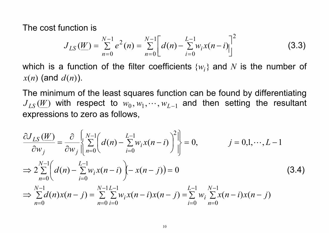
The cost function is

21

0

1

0

1

0

2 )()()()( ∑

∑ −−=∑=

−

=

−

=

−

=

N

n

L

ii

N

nLS inxwndneWJ (3.3)

which is a function of the filter coefficients }{ iw and N is the number of )(nx (and )(nd ).

The minimum of the least squares function can be found by differentiating )(WJLS with respect to ,,, 110 −Lwww L and then setting the resultant

expressions to zero as follows,

( )

∑ ∑ −−∑ =∑ −−=∑ −⇒

=−−∑

∑ −−⇒

−==

∑

∑ −−

∂∂

=∂

∂

−

=

−

=

−

=

−

=

−

=

−

=

−

=

−

=

−

=

1

0

1

0

1

0

1

0

1

0

1

0

1

0

1

0

21

0

)()()()()()(

0)()()(2

1,,1,0,0)()()(

L

i

N

ni

N

n

L

ii

N

n

N

n

L

ii

N

n

L

ii

jj

LS

jnxinxwjnxinxwjnxnd

jnxinxwnd

Ljinxwndww

WJL

(3.4)

10

Denote

Tdxdxdxdxdx LRLRRRR )]1(ˆ)2(ˆ)1(ˆ)0(ˆ[ˆ +−+−−= L (3.5)

where

1,,1,0,)()()(ˆ 1

0−=∑ −=−

−

=LjjnxndjR

N

ndx L

and

+−+−+−−+−+−

−+−+−−

=

)1,1(ˆ)1,1(ˆ)1,0(ˆ)2,0(ˆ

)1,0(ˆ)0,1(ˆ)0,2(ˆ)0,1(ˆ)0,0(ˆ

ˆ

LLRLRLRLR

RLRLRRR

R

xxxxxx

xx

xx

xxxxxxxx

xx

O

MOL

O

L

where

∑ −−=−−−

=

1

0)()(),(ˆ N

nxx jnxinxjiR

11

In practice, for stationary signals, we use

−−−

+−+−−

=

)0(ˆ)2(ˆ)1(ˆ)2(ˆ

)1(ˆ)1(ˆ)2(ˆ)1(ˆ)0(ˆ

ˆ

xxxxxx

xx

xx

xxxxxxxx

xx

RLRLRLR

RLRLRRR

RO

MOL

O

L

(3.6)

where

)(ˆ)()()(ˆ 1

0iRinxnxiR xx

iN

nxx −=+∑=

−−

=

As a result, we have

( ) dxxxLS

LSxxdx

RR

WRR

ˆ

ˆˆ1

⋅

⋅=−W ˆ=⇒

(3.7)

ˆprovided that xxR is nonsingular.

12

Example 3.1

Σ h zi=0

4

i-i

Σ w zi=0

4

i-i

Σ

x(n)

d(n)

y(n) e(n)

+

-

Unknown System

Σq(n)+

+

In this example least squares filtering is applied in determining the impulse response of an unknown system. Assume that the unknown impulse response is causal and {h }={1,2,3,2,1}. Given i N samples of )(nx and )(nd where )(nq is a measurement noise.

13

We can use MATLAB to simulate the least squares filter for impulse response estimation. The MATLAB source code is as follows,

%define the number of samples N=50;

%define the noise and signal powers noise_power = 0.0; signal_power = 5.0;

%define the unknown system impulse response h=[1 2 3 2 1];

%generate the input signal which is a Gaussian white noise with power 5 x=sqrt(signal_power).*randn(1,N);

14

%generate R_xx corr_xx=xcorr(x); for i=0:4 for j=0:4 R_xx(i+1,j+1)= corr_xx(N+i-j); end end

%generate the desired output plus noise d=conv(x,h); d=d(1:N)+sqrt(noise_power).*randn(1,N);

%generate R_dx corr_xd = xcorr(d,x); for i=0:4 R_dx(i+1) = corr_xd(N-i); end

%compute the estimate channel response W_ls = inv(R_xx)*(R_dx)'

15

−−

−−

=

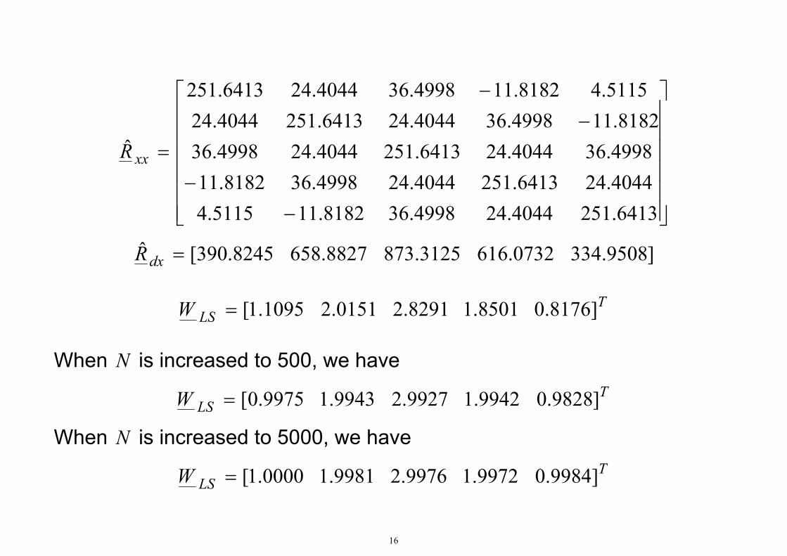
6413.2514044.244998.368182.115115.44044.246413.2514044.244998.368182.114998.364044.246413.2514044.244998.368182.114998.364044.246413.2514044.24

5115.48182.114998.364044.246413.251

ˆxxR

]9508.3340732.6163125.8738827.6588245.390[ˆ =dxR

TLSW ]8176.08501.18291.20151.21095.1[=

When N is increased to 500, we have

TLSW ]9828.09942.19927.29943.19975.0[=

When N is increased to 5000, we have

TLSW ]9984.09972.19976.29981.10000.1[=

16

When 500=N and the noise power is 0.5 (SNR=10 dB), we have

TLSW ]9925.09773.19728.29826.10158.1[=

When 500=N and the noise power is 5.0 (SNR=0 dB), we have

TLSW ]0591.10249.29484.20138.20900.1[=

It is observed that 1. The estimation accuracy improves as N increases. It is reasonable

because as N increases, the accuracy of xxR̂ and dxR̂ increases due to more samples are involved in their computation.

2. The estimation accuracy improves as the noise power decreases.

17

Example 3.2

Find the least squares filter of the following one-step predictor system:

s(n)

zz-1 Σ-b + b z-110

+

e(n)

d(n)

x(n)

where )12/2sin(2)( nns π=

−π

=−=12

)1(2sin2)1()( nnsnx

)()( nsnd =

18

Given , the aim is to find and in least squares sense. )(nd 0b 1b The MATLAB source code is as follows,

N=50; %define the number of samples

n=0:N-1; d=sin(2.*pi.*n./12); %generate d(n) x= d(2:N); %generate x(n) from d(n) d=d(1:N-1); %keep lengths of x(n) and d(n) equal corr_xx=xcorr(x,’unbiased’); %unbiased estimate of correlation for i=0:1

for j=0:1 R_xx(i+1,j+1)= corr_xx(N-1+i-j);

end end

19

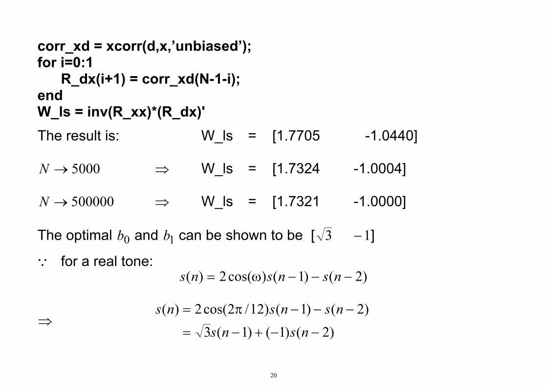
corr_xd = xcorr(d,x,’unbiased’); for i=0:1

R_dx(i+1) = corr_xd(N-1-i); end W_ls = inv(R_xx)*(R_dx)'

The result is: W_ls = [1.7705 -1.0440]

5000→N W_ls = [1.7324 -1.0004] ⇒

500000→N W_ls = [1.7321 -1.0000] ⇒ The optimal and can be shown to be [0b 1b 13 − ]

Q for a real tone:

)2()1()cos(2)( −−−ω= nsnsns

⇒ )2()1()1(3

)2()1()12/2cos(2)(−−+−=

−−−π=

nsnsnsnsns

20

Wiener Filtering The cost function to be minimized is )}({)( 2 neEWJMMSE (3.8) = Following the derivations in the least squares filter, the minimum of

)(WJMMSE is found by

( )

{ } { }∑ −−=

∑ −−=−⇒

=

−−

∑ −−⇒

−==

∑ −−

∂∂

=∂

∂

−

=

−

=

−

=

−

=

1

0

1

0

1

0

21

0

)()()()()()(

0)()()(2

1,,1,0,0)()()(

L

ii

L

ii

L

ii

L

ii

jj

MMSE

jnxinxEwjnxinxwEjnxndE

jnxinxwndE

LjinxwndEww

WJL

(3.9)

21

Assume and are jointly stationary, we have )(nd )(nx

1,,1,0,)()(1

0−=∑ −=−

−

=LjjiRwjR

L

ixxidx L (3.10)

Define

Tdxdxdxdxdx LRLRRRR )]1()2()1()0([ +−+−−= L (3.11)

and

−−−

−−−

=

)0()1()2()1()1()2(

)2()1()1()2()1()0(

xxxxxxxx

xxxx

xxxx

xxxxxxxx

xx

RRLRLRRLR

LRRLRLRRR

R

L

O

MOM

O

L

(3.12)

As a result,

( ) dxxxMMSE

MMSExxdx

RRW

WRR

⋅=⇒

⋅=−1 (3.13)

provided that xxR is nonsingular.

22

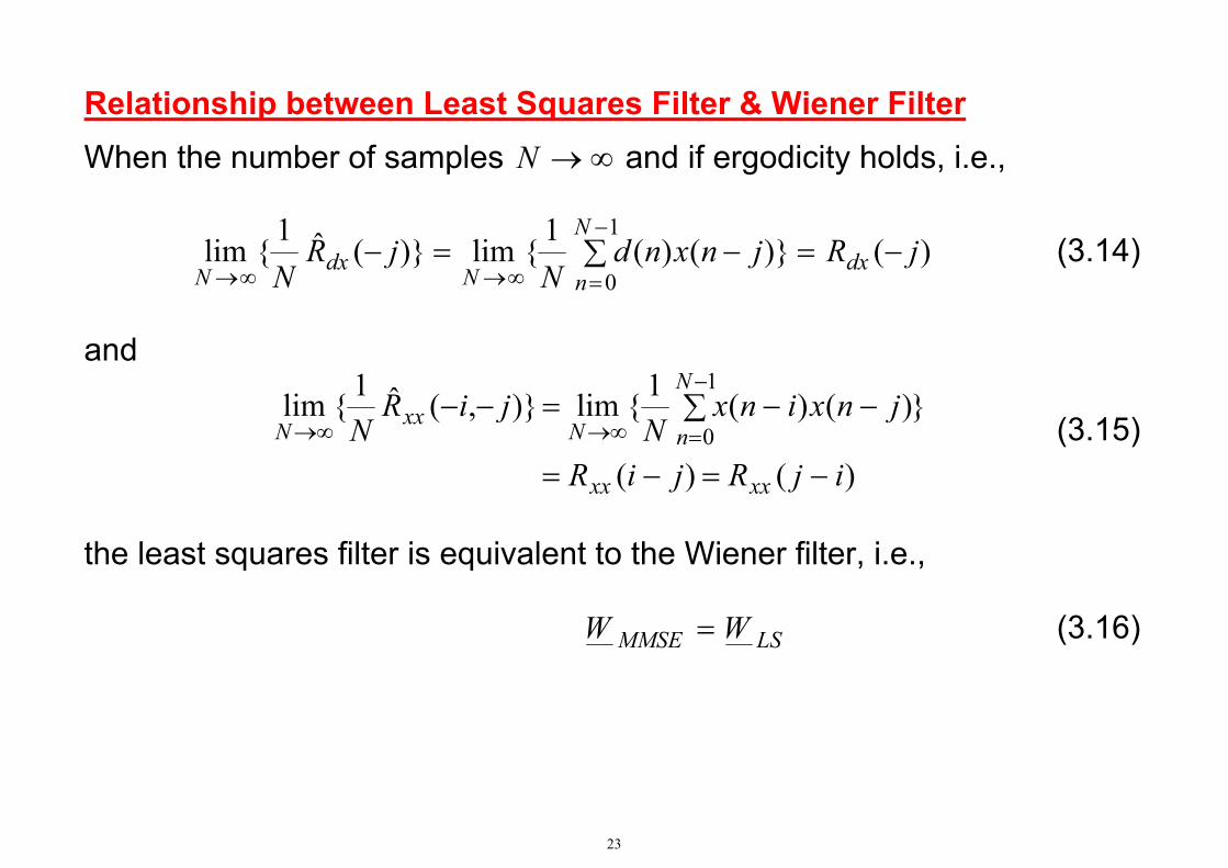
Relationship between Least Squares Filter & Wiener Filter

When the number of samples ∞→N and if ergodicity holds, i.e.,

∑ −=−=−−

=∞→∞→

1

0)()}()(

1{lim)}(ˆ1

{limN

ndx

Ndx

NjRjnxnd

NjR

N (3.14)

and

)()(

})()(1{lim)},(ˆ1{lim1

0

ijRjiR

jnxinxN

jiRN

xxxx

N

nNxx

N

−=−=

∑ −−=−−−

=∞→∞→ (3.15)

the least squares filter is equivalent to the Wiener filter, i.e., LSMMSE (3.16) WW =

23

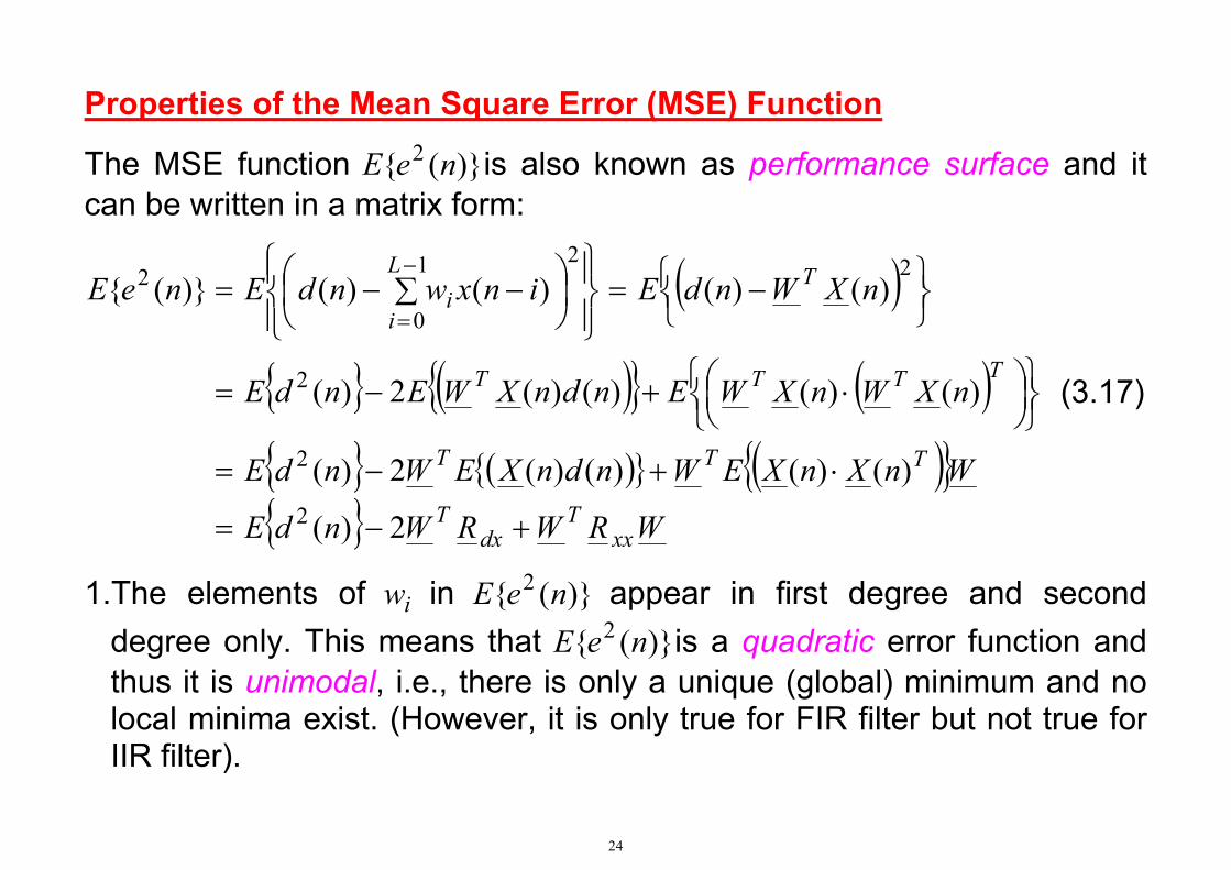
Properties of the Mean Square Error (MSE) Function

The MSE function is also known as performance surface and it can be written in a matrix form:

)}({ 2 neE

( )

{ } ( ){ } ( ){ } ( ){ } ( ){ }{ } WRWRWndE

WnXnXEWndnXEWndE

nXWnXWEndnXWEndE

nXWndEinxwndEneE

xxT

dxT

TTT

TTTT

TL

ii

+−=

⋅+−=

⋅+−=

−=

∑ −−=

−

=

2)(

)()()()(2)(

)()()()(2)(

)()()()()}({

2

2

2

221

0

2

(3.17)

1.The elements of in appear in first degree and second degree only. This means that 2 is a quadratic error function and thus it is unimodal, i.e., there is only a unique (global) minimum and no local minima exist. (However, it is only true for FIR filter but not true for IIR filter).

iw )}({ 2 neE{eE )}(n

24

An example for is shown below: 2=L

25

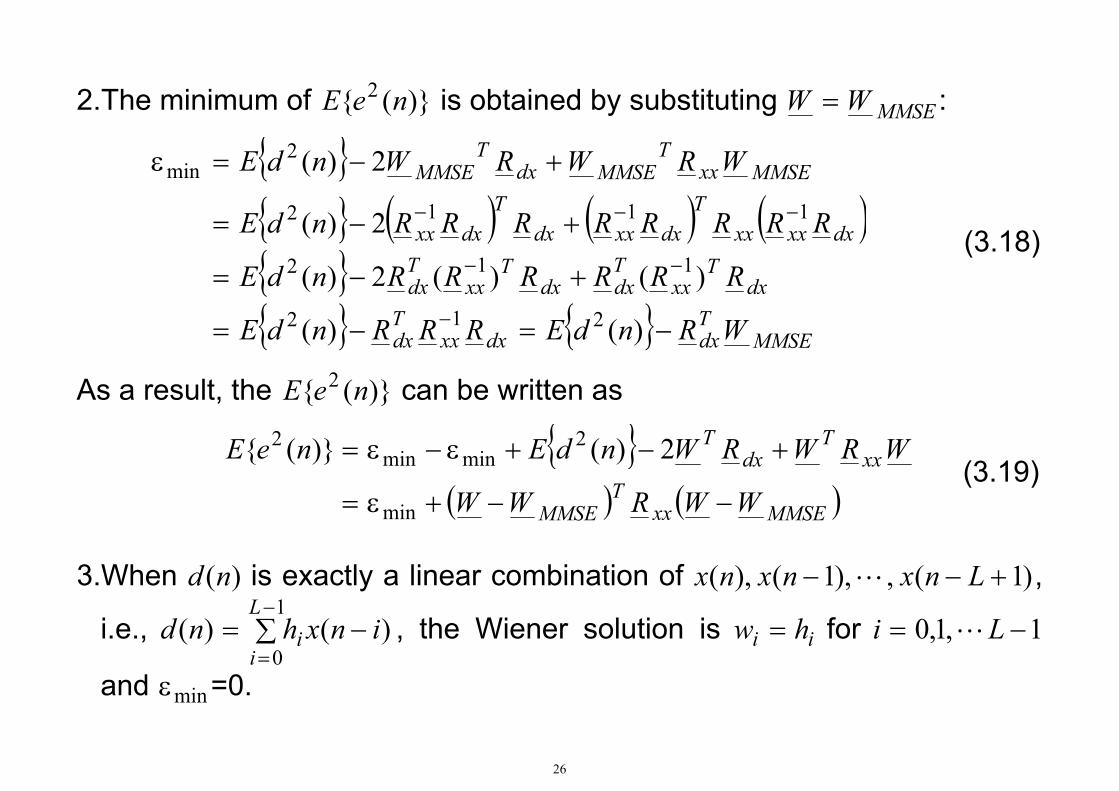
2.The minimum of is obtained by substituting )}({ 2 neE MMSEWW = :

{

}{ } ( ) ( ) ( ){ }{ } { } MMSE

Tdxdxxx

Tdx

dxT

xxTdxdx

Txx

Tdx

dxxxxxT

dxxxdxT

dxxx

MMSExxT

MMSEdxT

MMSE

WRndERRRndE

RRRRRRndE

RRRRRRRRndE

WRWRWndE

−=−=

+−=

+−=

+−=ε

−

−−

−−−

)()(

)()(2)(

2)(

2)(

212

112

1112

2min

(3.18)

As a result, the can be written as )}({ 2 neE

{

}

( ) ( )MMSExxT

MMSE

xxT

dxT

WWRWW

WRWRWndEneE

−−+ε=

+−+ε−ε=

min

2minmin

2 2)()}({ (3.19)

3.When is exactly a linear combination of )(nd )1(,),1(),( +−− Lnxnxnx L

ii hw

,

i.e., −1L

, the Wiener solution is ∑ −=0

)((i

i inxhd =)n = for 1,1,0 −= Li L

and =0. minε

26

Example 3.3 Determine the performance surface and the Wiener filter coefficients of the following system,

zz-1

Σ

w1w0

x(n)

d(n)-- +

where

=

==

87

,2112

,42)}({ 2dxxx RRndE

27

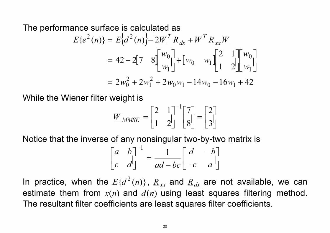
The performance surface is calculated as

{ } 2)()}({ 22 −= RWndEneE T

[ ] [ ]

421614222

2112

87242

101021

20

1

010

1

0

+−−++=

+

−=

+

wwwwww

ww

wwww

WRW xxT

dx

While the Wiener filter weight is

=

=

−

32

87

2112 1

MMSEW

Notice that the inverse of any nonsingular two-by-two matrix is

−1

−

−

−=

acbd

bcaddcba 1

In practice, when the )}({ 2 ndE , xxR and dxR are not available, we can estimate them from (x and (n using least squares filtering method. The resultant filter coefficients are least squares filter coefficients.

)n d )

28

Example 3.4

Find the Wiener filter of the following system:

s(n)

zz-1 Σ-b + b z-110

+

e(n)

d(n)

x(n)

where )12/2sin(2)( nns π= .

It can be seen that

−π

=12

)1(2sin2)(

nnx and

π

==122

sin2)()(n

nsnd .

The required statistics )0(xxR , )1(xxR , )0(dxR and )1(−dxR are computed as follows.

29

Using

2)2cos(1

)(sin 2 AA

−=

and

( ))cos()cos(21

)sin()sin( BABABA +−−=

then

( )

( ) 1})1(4{cos12

))1(2(2cos12

12)1(2sin2

12)1(2sin2)0(

=−π+=

−π−

=

−π

⋅

−π

=

nE

nE

nnERxx

30

23

122cos

122

12)1(2cos

122

12)1(2cos

122sin2

12)1(2sin2)1(

=

π−

=

π

+−π

−

π

−−π

=

π

⋅

−π

=

nnnnE

nnERxx

21

124

cos122

sin212

)2(2sin2)1(

23

122

sin212

)1(2sin2)0(

=

π−

=

π

⋅

−π

=−

=

π

⋅

−π

=

nnER

nnER

dx

dx

As a result,

−

=

=

−

13

2123

123

23

1~~

1

1

0

bb

31

The performance surface is given by

{ }

[ ]

133

123

23

1

21

23

21

2)()}({

101021

20

1

010

1

0

22

+−−++=

⋅

⋅+

⋅

−=

+−=

bbbbbb

bb

bbbb

WRWRWndEneE xxT

dxT

Notice that Moreover, the minimum MSE is computed as

.1)}({)}({ 22 == nxEndE

{ }0

21

23

113

21

23

1

)(2min

=+−=

−

⋅

−=

−=ε MMSETdxWRndE

This means that the optimal predictor is able to shift the phase of the delayed sine wave and achieve exact cancellation, resulting in 0min =ε

32

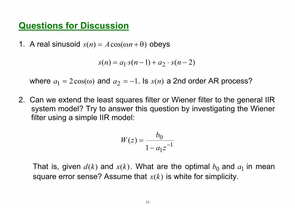
Questions for Discussion 1. A real sinusoid )cos()( θ+ω= nAns obeys

)2()1()( 21̀ −⋅+−= nsansans

where )cos(21 ω=a and 12 −=a . Is )(ns a 2nd order AR process? 2. Can we extend the least squares filter or Wiener filter to the general IIR

system model? Try to answer this question by investigating the Wiener filter using a simple IIR model:

11

0

1)(

−−=

za

bzW

That is, given )(kd and )(kx . What are the optimal and in mean square error sense? Assume that )(

0b 1akx is white for simplicity.

33

W(z)x(k) Σ

y(k)d(k)

EstimationError

+-

InputSignal

Output

e(k)

DesiredResponse

Steps:

(i) develop )(ke (ii) compute )}({ 2 keE in terms of xxR and dxR only. (iii) differentiate )}({ 2 keE w.r.t. and 0b 1a

34

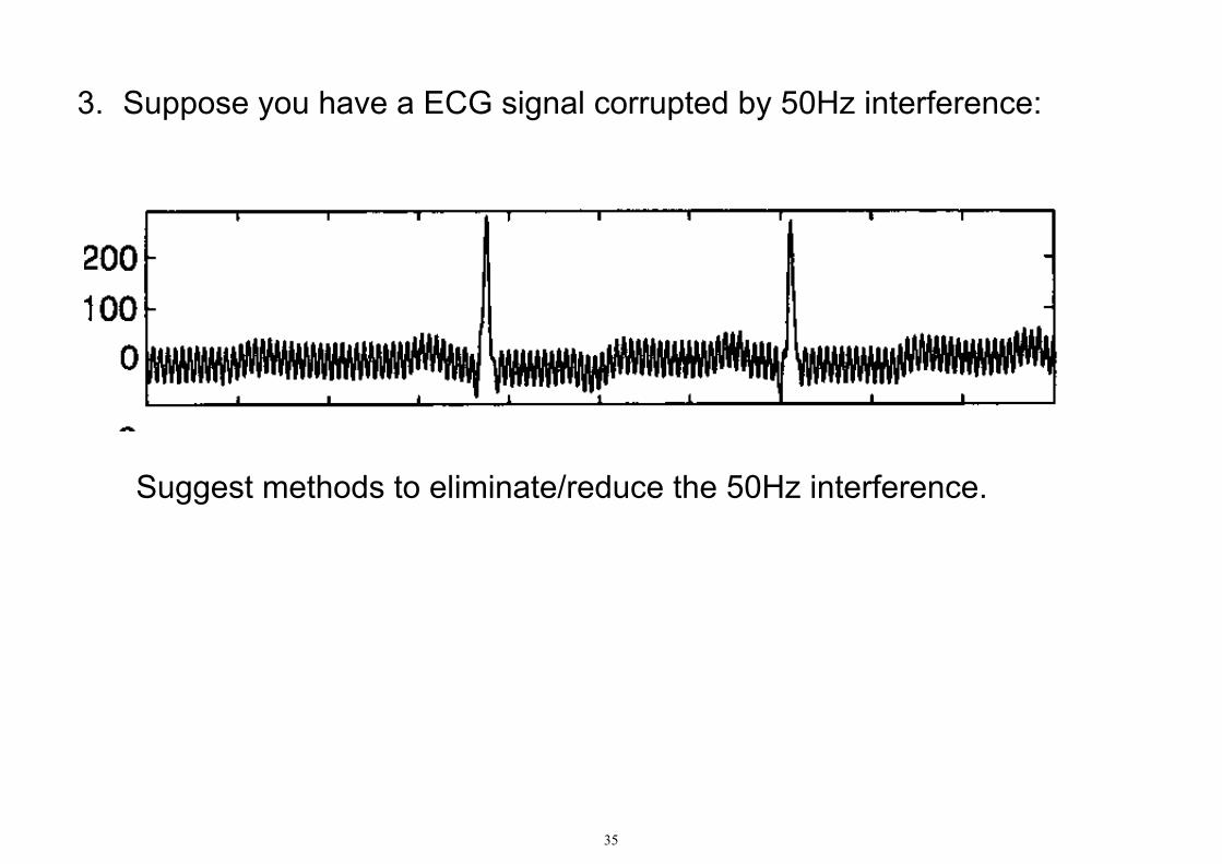
3. Suppose you have a ECG signal corrupted by 50Hz interference:

Suggest methods to eliminate/reduce the 50Hz interference.

35