Optimal Frequency for Wireless Power Transmission over

Dispersive Tissue

Ada S. Y. Poon∗, Stephen O’Driscoll†, and Teresa H. Meng‡

March 8, 2008

Abstract

Conventional wisdom in wireless power transmission over dispersive tissue tends to

operate at frequency less than 10 MHz due to tissue absorption loss. In the past half

century, analyses, circuit design techniques, and prototype implementation of wireless

power link for medical implants are developed entirely in this low-frequency range. This

paper re-examines the optimal frequency for the operation of these wireless interfaces.

It carries out full-wave analysis and shows that the optimal frequency is about 2 order

of magnitude higher than the conventional wisdom. Consequently, the efficiency can be

improved by 30 dB by operating at the optimal frequency. Alternatively, the receive

area can be reduced by 100 times for a given efficiency.

1 Introduction

Between 1960s and 1980s, several detailed studies of wireless power transmission for medical

implants were carried out [1–5]. They focused on the operation at frequencies below 20 MHz.

Transformer model and quasi-static analysis were therefore used in these studies. Based on

their results, circuit design techniques including tuning configurations [4,6–11] and geometry∗Ada S. Y. Poon is with the Department of Electrical and Computer Engineering, University of Illinois

at Urbana-Champaign, poon@uiuc.edu†Stephen O’Driscoll is with the Department of Electrical Engineering, Stanford University, stio-

fan@stanford.edu‡Teresa H. Meng is with the Department of Electrical Engineering, Stanford University, thm@stanford.edu

1

optimization [12] were developed in the late 1970s through 1990s. All these design techniques

were based on the transformer model and the principle of inductive coupling. In the past ten

years, some of these techniques have been applied to the implementation of highly integrated

implantable microsystems [13, 14]. Their transmission frequencies are all below 10 MHz.

Presumably, throughout the development of wireless power transmission over body tissue,

the optimal frequency range is below 10 MHz. However, we cannot find any vigorous proof

of this rule of thumb.

The choice of the transmission frequency is a trade-off between miniaturization and tis-

sue absorption. The amount of received power increases with increasing rate of change of

the transmitting field, that is, higher transmission frequency delivers more received power.

In other words, we can use a smaller receiver at higher frequency for a fixed received power.

However, body tissue is dispersive. Higher frequency incurs more tissue absorption. Con-

sequently, there is an optimal transmission frequency on the power transfer efficiency. Our

objectives are to find this optimal frequency, and to investigate how the optimal frequency

affects by the depth of the implant inside the body, the layered structure of tissue, and the

dimension of the transmitter.

To ensure our derivation on the power transfer efficiency is valid over a wide frequency

range, we need to devise the power transmission model that is not based on the transformer

model. Because the transformer model is a low-frequency approximation which is not

adequate to conclude the power transfer efficiency at higher frequencies. Indeed, we will

show that the conclusion draw from this low-frequency approximation does not favor the

operation at higher frequencies.

Based on the devised model, we will first consider a dispersive homogeneous medium.

We carry out full-wave analysis and show that the optimal transmission frequency is in

the GHz-range for typical biological tissue dielectric properties. The frequency is at least

2 order of magnitude higher than the conventional wisdom. Furthermore, we show that

the optimal power transfer efficiency is inversely proportional to the cube of the depth of

implant inside body. This implies that the regime for optimal power transmission is in

between the far field and the near field.

Our analysis in the homogeneous medium brings out that the dispersiveness of body

2

tissue is not as worse as conventional wisdom believed. Next, we will include the inhomoge-

neous nature of body tissue and investigate its effect on the optimal frequency. Scattering

from tissue interfaces reduces the optimal frequency. However, the optimal frequency re-

mains in the GHz-range. It is relatively invariant with the implant depth and the orientation

of the receiver. Scattering also reduces the optimal efficiency by almost an order of mag-

nitude. However, the efficiency remains inversely proportional to the cube of the implant

depth.

In our analyses, we consider the scenario where the dimension of the implantable device

is small relative to the depth of the implant inside the body, for example, a 2-mm width coil

at a depth of 2 cm. Therefore, we use point sources to model both the transmitter and the

receiver. Finally, we will verify this point-source approximation by full-wave electromagnetic

simulation using finite sized sources. We use Zeland IE3D [15] which is a solver based on

method of moment. The simulated results match well with the theoretical ones. In addition,

we also investigate how the transmitter dimension affects the optimal frequency. Larger

dimension reduces the optimal frequency. For a practical dimension of the transmitter, the

optimal frequency is in the sub-GHz range. Compared with the conventional wisdom, the

optimal frequency is about 2 order of magnitude higher. For a fixed received power, the

receive area can be reduced by 106 times. For a fixed receive area, the efficiency can be

improved by 30 dB including scattering loss. For a fixed efficiency, the receive area can be

reduced by 100 times.

The rest of the paper is organized as follows. Section 2 presents the power transmission

model. Section 3 derives the optimal transmission frequency in dispersive homogeneous

medium. Section 4 extends the analysis to inhomogeneous layered medium. Section 5

verifies the analytical results and the numerical examples by full-wave electromagnetic sim-

ulations. Finally, we will conclude this paper in Section 6.

In the following, we use boldface letters for vectors and boldface letters with a bar G

for matrices. For a vector v, v denotes its magnitude and v is a unit vector denoting

its direction. (·)∗ and (·)† denote the conjugate and the conjugate-transpose operations

respectively. For a complex number z, Re z and Im z denote the real and the imaginary

parts respectively. The relation f(x) ∼ g(x) means that limx→∞f(x)g(x) is a constant.

3

ZI AreaA

Figure 1: A receive current loop connected to a load Z.

2 Modeling of Power Transmission

As current loops are usually used in the wireless powering of implants, it is more convenient

to consider magnetic current density as sources. In addition, we assume that all fields and

sources have a time dependence e−iωt. Electromagnetic fields due to the transmit magnetic

current density Jm,1(r) and the receive magnetic current density Jm,2(r) in a medium of

relative permittivity εr and conductivity σ satisfy

∇×H = −iωε0εrE + σE (1a)

∇×E = iωµ0H− Jm,1 − Jm,2 (1b)

Substituting them into the Poynting vector yields

∇ · (E×H∗) = iωµ0|H|2 − iωε0εr|E|2 − σ|E|2 −H∗ · Jm,1 −H∗ · Jm,2 (2)

Rearranging terms, we relate the transmitted power to the received power plus losses:

−H∗ · Jm,1 = ∇ · (E×H∗) + iωµ0|H|2 − iωε0ε∗r |E|2 + σ|E|2 + H∗ · Jm,2 (3)

The term on the left is the complex transmitted power. On the right, ∇ · (E × H∗) is

the radiation loss; ωε0 Im εr|E|2 is the dielectric loss; σ|E|2 is the induced-current loss; and

H∗ · Jm,2 is the complex received power. We define the power transfer efficiency η as the

ratio of real received power to tissue absorption (dielectric loss plus induced-current loss),

that is,

η :=Pr

Pl=

Re∫

H∗(r) · Jm,2(r) dr∫ [ωε0 Im εr(r) + σ(r)

]∣∣E(r)∣∣2 dr

(4)

The integration in the numerator is over the received volume while the integration in the

denominator is over the tissue volume.

4

As Jm,2(r) is induced by H(r) over the received volume, we want to relate Jm,2(r) to

H(r). Consider the receive current loop shown in Fig. 1. The total magnetic flux incident

on the receive loop is µ0

∫rx loop H(r) · n ds where n denotes the orientation of the receive

loop. The rate of change of this total magnetic flux yields the induced emf. This induced

emf is the voltage across Z. The current is therefore given by

I =iωµ0

Z

∫rx loop

H(r) · n ds (5)

The direction of Jm,2(r) is n. From definition, its magnitude Jm,2(r) relates to the induced

magnetic moment density as

Jm,2(r) = −iωµ0IA (6a)

=ω2µ2

0A

Z

∫rx loop

H(r) · n ds (6b)

We consider area-constrained implantable devices so we model the receiver as a point source.

Thus, we have

Jm,2(r) =ω2µ2

0A2

ZH(−zd2) · n δ(r + zd) (7)

where −zd is the location of the receiver. Substituting it into (4) yields

η =ω2µ2

0A2/Z

∣∣H(−zd) · n∣∣2∫ [

ωε0 Im εr(r) + σ(r)]∣∣E(r)

∣∣2 dr(8)

The power transfer efficiency is now in terms of the incident magnetic field at −zd and

the electric field over the tissue volume. In the following, we will first derive these fields

due to a transmit vector point source in a dispersive homogeneous medium and study how

the efficiency varies with frequency. Then, we will replace the homogeneous medium with

a layered tissue model, and carry out the same study. Finally, we will replace the point

sources with finite coils, and carry out electromagnetic simulation to verify the analytical

results based on point sources.

5

3 Vector Point Source in Homogeneous Medium

We model the transmitter as a vector point source. The magnetic and the electric fields

can be represented by a basis set consisting of 6 vector elements:

M1m(r) = ∇×[rh(1)

n (kr)Ynm(θ, φ)], m = −1, 0, 1 (9a)

N1m(r) =1k∇×∇×

[rh(1)

n (kr)Ynm(θ, φ)], m = −1, 0, 1 (9b)

where k2 = ω2µ0ε0(εr + i σ

ωε0

). These basis elements correspond to the lowest order modes

in spherical multipole expansion of the daydic Green’s functions in homogeneous medium.

Specifically, N10(r) and M10(r) are the respective magnetic field and electric field due

to an infinitesimal current loop oriented along the z-axis; 1√2N1,−1(r) − 1√

2N1,1(r) and

1√2M1,−1(r)− 1√

2M1,1(r) are the respective magnetic field and electric field due to a current

loop oriented along the x-axis; and i√2N1,−1(r) + i√

2N1,1(r) and i√

2M1,−1(r) + i√

2M1,1(r)

are the respective magnetic field and electric field due to a current loop oriented along the

y-axis. As the scattered field due to Jm2(r) is much weaker than the incident field due to

Jm,1(r), the magnetic and the electric fields can be expressed as

H(r) = −k3[α−1N1,−1(r) + α0N1,0(r) + α1N1,1(r)

](10a)

E(r) = −iωµ0k2[α−1M1,−1(r) + α0M1,0(r) + α1M1,1(r)

](10b)

where (α−1, α0, α1) ∈ C3 denotes the orientation of the transmit coil.

Now, the received power and the tissue absorption can be written in terms of αm’s.

For a given orientation of the receive coil n, we will first derive the optimal power transfer

efficiency that maximizes over all possible orientations of the transmit coil, αm’s. Then,

we will analyze this optimal power transfer efficiency under different approximations and

dielectric models.

3.1 Optimal Power Transfer Efficiency

Suppose the transmitter is at the origin, the tissue volume spans z < −d1, and the receiver

is at −d2. Then, the tissue absorption is

Pl =ωµ0|k|4 Im k2

2

∫tissue

∣∣α−1M1,−1(r) + α0M1,0(r) + α1M1,1(r)∣∣2 dr (11)

6

The symmetry in φ of the tissue volume implies that the cross terms are zero. Therefore,

we have

Pl =ωµ0|k|4 Im k2

2

∫tissue

|α−1|2∣∣M(3)

1,−1(r)∣∣2 + |α0|2

∣∣M(3)1,0(r)

∣∣2 + |α1|2∣∣M(3)

1,1(r)∣∣2 dr (12)

For the received power, we expand the orientation of the receive coil as

n = β−1N1,−1(−zd2)|N1,−1(−zd2)|

+ β0N1,0(−zd2)|N1,0(−zd2)|

+ β1N1,1(−zd2)|N1,1(−zd2)|

(13)

for some βm’s satisfying |β−1|2 + |β0|2 + |β1|2 = 1. The directions of N1,−1(−zd2) and

N1,1(−zd2) are orthogonal and lie on the xy-plane, while the direction of N1,0(−zd2) is z.

The received power becomes

Pr =ω2µ2

0|k|6A2

2Z

∣∣∣α−1β∗−1

∣∣N1,−1(−zd2)∣∣ + α0β

∗0

∣∣N1,0(−zd2)∣∣ + α1β

∗1

∣∣N1,1(−zd2)∣∣∣∣∣2 (14)

Now, we maximize the power transfer efficiency over all possible orientations of the

transmit coil. The optimal power transfer efficiency is given by

ηopt =ωµ0|k|2A2

Z Im k2

[ ∣∣β−1N1,−1(−zd2)∣∣2∫

tissue

∣∣M1,−1(r)∣∣2 dr

+

∣∣β0N1,0(−zd2)∣∣2∫

tissue

∣∣M1,0(r)∣∣2 dr

+

∣∣β1N1,1(−zd2)∣∣2∫

tissue

∣∣M1,1(r)∣∣2 dr

](15)

and the corresponding orientation of the transmit coil is

αm =|N1,m(−zd2)

∣∣∫tissue

∣∣M1,m(r)∣∣2 dr

βm, m = −1, 0, 1 (16)

The proof is included in Appendix A. Furthermore, from definitions in (9), we obtain∫tissue

∣∣M1,−1(r)∣∣2 dr =

∫tissue

∣∣M1,1(r)∣∣2 dr

=e−2kId1

16|k|4d1

[9− 14kId1 + 2k2

Id21 − 4k3

Id31 + 8|k|2d2

1

( 1kId1

− 14

+kId1

2)]

+Ei(−2kId1)

4|k|4d1

[|k|2d2

1

(3 + 2k2

Id21

)− 2k2

Id21

(3 + k2

Id21

)](17a)∫

tissue

∣∣M1,0(r)∣∣2 dr =

e−2kId1

8|k|4d1

[3− 10kId1 − 2k2

Id21 + 4k3

Id31 + 4|k|2d2

1

( 1kId1

+12− kId1

)]+

Ei(−2kId1)2|k|4d1

[|k|2d2

1

(3− 2k2

Id21

)− 2k2

Id21

(3− k2

Id21

)](17b)

and ∣∣N1,−1(−zd2)∣∣2 =

∣∣N1,1(−zd2)∣∣2

=3e−2kId2

4π|k|6d62

[1− |k|2d2

2 + |k|4d42 + 2kId2

(1 + 2kId2 + |k|2d2

2

)](18a)

∣∣N1,0(−zd2)∣∣2 =

3e−2kId2

π|k|6d62

(1 + 2kId2 + |k|2d22) (18b)

7

where kI = Im k and Ei(·) is the exponential integral function.

From (16), it is not necessary to orient the transmit coil along the same direction as

the receive coil for maximum power delivery. There are certain directions where the tissue

absorption is less, while there are some directions where the received power is more. The

optimal orientation is a trade-off between them and this trade-off varies with frequency. This

is the reason why we study the variation of the efficiency with frequency that is optimized

over all possible transmit orientation.

3.2 Static and Quasi-static Approximations

At DC, ω = 0, and therefore |k| = kI = 0 and Im k2/(ωµ0) = σ. We have

|k|2∣∣N1,−1(−zd2)

∣∣2∫tissue

∣∣M1,−1(r)∣∣2 dr

=|k|2

∣∣N1,1(−zd2)∣∣2∫

tissue

∣∣M1,1(r)∣∣2 dr

=4d1

3πd62

(19a)

|k|2∣∣N1,0(−zd2)

∣∣2∫tissue

∣∣M1,0(r)∣∣2 dr

=8d1

πd62

(19b)

The static optimal power transfer efficiency is

ηopt,0 =4d1A

2/Z

3πσd62

(|β−1|2 + 6|β0|2 + |β1|2

)(20)

The optimal efficiency is independent of frequency. It is maximized when |β0| = 1 and

|β−1| = |β1| = 0, that is, the receive coil is oriented along z.

At low frequency, the displacement current −iωε0εrE is small. Quasi-static approxima-

tion neglects this current which is equivalent to setting εr equal to 0. The wavenumber is

then given by

k =√

ωµ0σ

2(1 + i) (21)

This yields

|k|2 = 2k2I = ωµ0σ

Suppose d1 is much smaller than the skin depth, that is, kId1 1. Then,

|k|2∣∣N1,−1(−zd2)

∣∣2∫tissue

∣∣M1,−1(r)∣∣2 dr

=|k|2

∣∣N1,1(−zd2)∣∣2∫

tissue

∣∣M1,1(r)∣∣2 dr

=4d1

3πd42

(|k|2d2

2 +√

2|k|d2 + 1)|k|2e−2kId2 + o

(|k|2e−2kId2

)(22a)

|k|2∣∣N1,0(−zd2)

∣∣2∫tissue

∣∣M1,0(r)∣∣2 dr

=8d1

πd42

|k|2e−2kId2 + o(|k|2e−2kId2

)(22b)

8

as ω →∞. The quasi-static optimal efficiency is

ηopt =4d1A

2/Z

3πσd42

[6|β0|2 +

(|k|2d2

2 +√

2|k|d2 + 1)(|β−1|2 + |β1|2

)]|k|2e−2kId2 (23)

+ o(|k|2e−2kId2

)In terms of the static optimal efficiency,

ηopt = ηopt,0 e−2kId2 · |k|2d22

[1 +

|β−1|2 + |β1|2

|β−1|2 + 6|β0|2 + |β1|2(|k|2d2

2 +√

2|k|d2

)](24)

+ o(|k|2e−2kId2

)As kI ∝

√ω, the optimal efficiency decreases exponentially with

√ω. Therefore, it is worse

to operate at higher frequencies than at DC. We believed that this is also the source for the

conventional wisdom of operating below 10 MHz.

3.3 Full-wave Analysis without Relaxation Loss

Including the displacement current, the wavenumber becomes

k = ω√

µ0ε0εr + iσ

2

õ0

ε0εr+ o(1) (25)

as ω →∞. This yields

kI =σ

2

õ0

ε0εr+ o(1) |k| = ω

√µ0ε0εr + o(ω) (26)

Now kI is asymptotically invariant with frequency. Similarly, we assume that d1 is much

smaller than the skin depth, that is, kId1 1. Then

|k|2∣∣N1,−1(−zd2)

∣∣2∫tissue

∣∣M1,−1(r)∣∣2 dr

=|k|2

∣∣N1,1(−zd2)∣∣2∫

tissue

∣∣M1,1(r)∣∣2 dr

=3kIe

−2kId2

2πd42

(|k|2d2

2 + 2kId2 − 1)

+ o(1) (27a)

|k|2∣∣N1,0(−zd2)

∣∣2∫tissue

∣∣M1,0(r)∣∣2 dr

=6kIe

−2kId2

πd42

+ o(1) (27b)

as ω →∞. The optimal efficiency is

ηopt =3kIe

−2kId2A2/Z

2πσd42

[4|β0|2 +

(|k|2d2

2 + 2kId2 − 1)(|β−1|2 + |β1|2

)]+ o(1) (28)

9

In contrast to the optimal efficiency obtained from quasi-static analysis, the efficiency from

full-wave analysis increases with frequency asymptotically. This difference in the conclusions

illustrates that current analysis techniques for wireless power transmission over body tissue

are not adequate.

3.4 Full-wave Analysis including Relaxation Loss

The efficiency would not increase indefinitely with frequency. At high frequency, there are

loss mechanisms other than induced current. The dominant mechanism is the relaxation

loss [16]. Consequently, there will be an optimal transmission frequency. We are interested

in finding where it is, in the MHz-range or in the GHz-range. If it is in the MHz-range,

quasi-static approximation would be sufficient. On the other hand, if it is in the GHz-

range, new analysis and new design techniques will be needed. To address this question, a

relaxation model is required.

From (3), the dielectric loss ωε0 Im εr|E|2 encapsulates the relaxation loss. As Im εr 6= 0,

Kramers-Kronig relations [17, Section 7.10] ensure that εr varies with frequency. Therefore,

dielectric relaxation is often modeled by a frequency-dependent relative permittivity. Debye

relaxation model and its variants are popular models for biological media. In this relaxation

model, the relative permittivity of the medium is expressed as [16]:

εr(ω) = ε∞ +εr0 − ε∞1− iωτ

+ iσ

ωε0(29)

The imaginary component of εr(ω) includes the static conductivity σ. That is, the dielectric

loss in this model includes both relaxation loss and induced-current loss. In the expression,

ε∞ is the relative permittivity at frequencies where ωτ 1, while εr0 is the relative per-

mittivity at ωτ 1. This model is valid for frequency much less than 1/τ . For example,

over the frequency range of 2.8 MHz f 140 GHz, the parameters for muscle are:

τ = 7.23 ps, ε∞ = 4, and εr0 = 54. Here, ε∞ is the relative permittivity at 140 GHz or

beyond, εr0 is the relative permittivity at 2.8 MHz, and the relaxation model is valid for

frequency much less than 1/τ = 140× 109 Hz.

In frequency region where ωτ 1, the relative permittivity is approximately equal to

εr(ω) ≈ εr0 +i

ωε0

(σ + ω2τε0∆ε

)(30)

10

where ∆ε = εr0 − ε∞. This yields

kI ≈σ + ω2τε0∆ε

2

õ0

ε0εr0|k| ≈ ω

√µ0ε0εr0 (31)

Now, kI increases slowly with frequency. The asymptotic efficiency can be obtained from

(28) by the following substitutions: εr → εr0 and σ → σ+ω2τε0∆ε. Defining kI0 = σ2

õ0

ε0εr0,

the asymptotic optimal efficiency can be written as

ηopt =3kI0e

−2kI0d2A2/Z

2πσd42

[(d22εr0

c2+

d2τ∆ε

c√

εr0

)(|β−1|2 + |β1|2

)ω2

+ 4|β0|2 − |β−1|2 − |β1|2 + 2kI0d2

(|β−1|2 + |β1|2

)]e− d2τ∆ε

c√

εr0ω2

+ o(1) (32a)

as ω →∞. The asymptotic term is maximized when

ωopt =

√√√√ c√

εr0

d2τ∆ε−

4|β0|2 − |β−1|2 − |β1|2 + 2kI0d2

(|β−1|2 + |β1|2

)(d22εr0

c2+ d2τ∆ε

c√

εr0

)(|β−1|2 + |β1|2

) (33)

If the transmit-receive separation is less than 2.5 times of the low-frequency skin depth,

that is, 2kI0d2 < 5, the asymptotic optimal frequency will be lower-bounded by

ωopt >

√√√√ c√

εr0

d2τ∆ε−

(|β−1|2 + |β1|2

)−1(d22εr0

c2+ d2τ∆ε

c√

εr0

) ≈

√c√

εr0

d2τ∆ε(34)

The approximation is due to d22εr0

c2 d2τ∆ε

c√

εr0in general. Gabriel et al. have experimentally

characterized dielectric properties of 17 different kinds of biological tissue [18]1. Table 1

lists the approximated lower bound for the 17 different tissues assuming d2 = 1 cm. All

lower bounds are in the GHz-range. Consequently, for any potential depth of implant inside

the body, the asymptotic optimal frequency is around the GHz-range for small transmit and

small receive sources.

As muscle is the most widely reported tissue, let us take muscle as an example. We

compute the exact optimal frequencies that maximize the efficiency given in (15) for different

transmit-receive separations, and compare them with the approximate lower bound in (34).

Fig. 2(a) shows these curves. The implant depth in the graph refers to d2 − d1. The1The parameters in [18] are for the 4-term Cole-Cole model which is a variant of the Debye relax-

ation model. Conversion to the Debye relaxation model is as follows: τ = τ1, εr0 = ∆ε1 + ε∞, and

σ =P4

n=2ε0∆εn

τn+ σs

11

Table 1: Summary of the approximate lower bound on the asymptotic optimal frequency

for 17 different kinds of biological tissue, assuming d2 = 1 cm.

Tissue type Approximate lower-bound

on fopt (GHz/cm−1/2)

Blood 3.54

Bone (cancellous) 3.80

Bone (cortical) 4.50

Brain (grey matter) 3.85

Brain (white matter) 4.23

Fat (infiltrated) 6.00

Fat (not infiltrated) 8.64

Heart 3.75

Kidney 3.81

Lens cortex 3.93

Liver 3.80

Lung 4.90

Muscle 3.93

Skin (dry) 4.44

Skin (wet) 4.01

Spleen 3.79

Tendon 3.17

12

ExactApprox. lower bound

1

3

4

Opt

imal

Fre

quen

cy (

GH

z)

2 3 4 5 6Implant Depth (cm)

2

6

8

10

ExactApprox. lower bound

10-5

10-3

10-2

10-1

Effi

cien

cy

2 3 4 5 6Implant Depth (cm)

10-4

(a) (b)

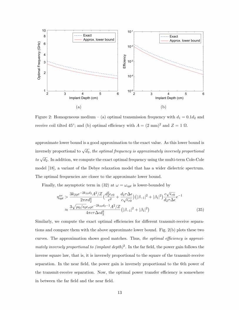
Figure 2: Homogeneous medium – (a) optimal transmission frequency with d1 = 0.1d2 and

receive coil tilted 45; and (b) optimal efficiency with A = (2 mm)2 and Z = 1 Ω.

approximate lower bound is a good approximation to the exact value. As this lower bound is

inversely proportional to√

d2, the optimal frequency is approximately inversely proportional

to√

d2. In addition, we compute the exact optimal frequency using the multi-term Cole-Cole

model [18], a variant of the Debye relaxation model that has a wider dielectric spectrum.

The optimal frequencies are closer to the approximate lower bound.

Finally, the asymptotic term in (32) at ω = ωopt is lower-bounded by

ηasopt >

3kI0e−2kI0d2A2/Z

2πσd42

(d22εr0

c2+

d2τ∆ε

c√

εr0

)(|β−1|2 + |β1|2

) c√

εr0

d2τ∆εe−1

≈3√

µ0/ε0εr0e−2kI0d2−1A2/Z

4πcτ∆εd32

(|β−1|2 + |β1|2

)(35)

Similarly, we compute the exact optimal efficiencies for different transmit-receive separa-

tions and compare them with the above approximate lower bound. Fig. 2(b) plots these two

curves. The approximation shows good matches. Thus, the optimal efficiency is approxi-

mately inversely proportional to (implant depth)3. In the far field, the power gain follows the

inverse square law, that is, it is inversely proportional to the square of the transmit-receive

separation. In the near field, the power gain is inversely proportional to the 6th power of

the transmit-receive separation. Now, the optimal power transfer efficiency is somewhere

in between the far field and the near field.

13

3.5 Trade-off between Receiver Miniaturization and Tissue Absorption

From (11) and (17), the tissue absorption can be written as

Pl =ωµ0|k|2 Im k2

2

|α0|2

[e−2kId1

4kI

(2 + kId1 − 2k2

Ik21

)+

d1Ei(−2kId1)2

(3− 2k2

Id21

)]+ (|α−1|2 + |α1|2)

[e−2kId1

8kI

(4− kId1 + 2k2

Id21

)+

d1Ei(−2kId1)4

(3 + 2k2

Id21

)]+ o(ω4) (36)

as ω → ∞. Therefore, Pl is approximately proportional to ω4. Similarly, from (14) and

(18), the received power can be written as

Pr =3ω2µ2

0|k|4A2 e−2kId2

8πd22Z

∣∣α−1β∗−1 + α1β

∗1

∣∣2 + o(ω6) (37)

as ω → ∞. Therefore, Pr is approximately proportional to ω6A2. Consequently, the

efficiency is approximately proportional to ω2A2. If the transmission frequency is increased

from 10 MHz to 1 GHz,

• the receive area will be reduced by 106 times for a fixed received power;

• the receive area will be reduced by 102 times for a fixed efficiency; and

• the efficiency will be increased by 104 times or 40 dB for a fixed receive area.

4 Point Source over Layered Medium

Conventional wisdom in wireless power transmission is to operate at lower frequency due

to tissue absorption loss. Our analyses over homogeneous medium, however, bring out that

the tissue absorption loss is not as worse as conventional wisdom believed. Next, we will

investigate the effect of scattering from the layered nature of tissue on the optimal frequency.

We consider planar interfaces and magnetic dipoles as sources (see Fig. 3). As the electric

and the magnetic fields are given in the form of Sommerfeld integrals [19, Sec. 2.3] and we

need to compute the fields near the sources, closed-form analyses as in the homogeneous

medium are not feasible. Alternately, we consider a multi-layer tissue model as illustrated in

Fig. 3 and numerically compute the Sommerfeld integrals. To accelerate the computation,

we follow [20] to deform the integration path. Furthermore, as the integrals involve Bessel

14

z

0

−d1

−d4

AirSkin

Fat

Muscle

−d2

−d3

Figure 3: A magnetic dipole on top of a multi-layer interface with the receive coil embedded

in the muscle layer.

functions which are oscillatory, we partition the revised integration path into sub-paths

with exponentially increasing length, and perform the integration over these sub-paths.

Fig. 4(a) plots the optimal frequency versus the implant depth for both air-muscle half

space and air-skin-fat-muscle multi-layer interface. In the latter case, the thickness of skin is

4.5 mm and the thickness of fat is 7.5 mm, that is, d2−d1 = 4.5 mm and d3−d2 = 7.5 mm.

The receive coil is tilted 45 with respect to the interface which is equivalent to setting

(β−1, β0, β1) = (1/2,√

1/2, 1/2). Note that in the previous section, the receiver is at −zd2

while in the multi-layer tissue model, it is at −zd4.

The optimal frequencies are less than those obtained assuming homogeneous medium.

This is due to the scattering from the interfaces. Optimal frequencies are relatively invariant

with implant depth, particularly in the multi-layer case. The optimal frequency for the

air-muscle half space is around 2 GHz and that for the multi-layer interface is around

1 GHz. That is, the optimal frequencies remain in the GHz-range. In addition, we compute

the optimal frequencies for various receive coil orientation, and find out that the optimal

frequencies are insensitive to the orientation which agrees with the prediction from (34).

Finally, we study how tissue interfaces affect the power transfer efficiency. Fig. 4(b)

plots the optimal efficiency versus the implant depth in the 3 different media. Scattering by

interfaces reduces the efficiency by almost an order of magnitude. The efficiency is slightly

better with more layers because scattering reduces tissue absorption more than received

power. The variation of the optimal efficiency with the implant depth, however, remains

15

0.5

1

2

3

4

10

6

0.8

2 3 4 5 6Implant Depth (cm)

Op

tim

al F

req

uen

cy (G

Hz)

Air-Muscle Air-Skin-Fat-Muscle

MuscleAir-Muscle Air-Skin-Fat-Muscle

Muscle

Effic

ien

cy

10−5

10−4

10−3

10−2

10−1

2 3 4 5 6Implant Depth (cm)

(a) (b)

Figure 4: Inhomogeneous medium – (a) optimal transmission frequency with d1 = 0.1d4

and receive coil tilted 45; and (b) optimal efficiency with A = (2 mm)2 and Z = 1 Ω.

approximately inversely proportional to (implant depth)3.

In conclusion, both received power and tissue absorption increase with frequency. At a

given frequency, tissue interfaces reduce both received power and tissue absorption; how-

ever, their ratio remains increasing with frequency initially. At the optimal frequency, the

dispersiveness of tissue dominates. The received power begins decreasing with increasing

frequency. Frequencies where tissue dispersiveness dominates, do not affect significantly by

the tissue interfaces. As a result, the conclusion on the optimal frequency for point sources

derived assuming homogeneous medium remains valid.

5 Finite Coil over Layered Medium

The analytical results and numerical examples presented are based on point sources. We

will verify the result using finite coils through electromagnetic simulations. To explain the

simulation results, we need to introduce the equivalent circuit for the power transmission

link first.

16

ZL

I1V2

I2V1

Figure 5: A single transmit and a single receive coil system

5.1 Equivalent Circuit Model

The mutual interaction between the two coils in Fig. 5 can be described by the impedance

equations:

V1 = Z11I1 + Z12I2

V2 = Z21I1 + Z22I2

When the load impedance ZL is conjugate matched to Z22,

I2 = − Z21

Z22 + ZL= − Z21

2R22I1

where Rnm is the real part of Znm for all n, m. In terms of the circuit parameters, the re-

ceived power Pr, the tissue absorption Pl, and the efficiency defined earlier can be expressed

as

Pr =12

Re ZL|I2|2 =|Z21|2

8R22|I1|2 Pl =

12(R11 −Rw)|I1|2 η =

|Z21|2

4(R11 −Rw)R22(38)

where Rw is the wire resistance of the transmit coil. The analytical results and numerical

examples presented in the previous two sections are based on point sources and therefore,

they do not include the ohmic loss in both coils. Furthermore, they do not take into account

the scattered field from the receive coil when deriving the electromagnetic fields in (10).

When we take into account both ohmic loss and scattered field from the receive coil, we

consider the input power to the system

Pin =12

Re(V1I∗1 ) =

12

Re(Z11 −

Z12Z21

Z22 + ZL

)|I1|2 =

12

[R11 −

Re(Z12Z21)2R22

]|I1|2 (39)

The difference Pin − Pr is the total dissipation power which includes tissue absorption due

to the sum of incident field from the transmit coil and the scattered field from the receive

17

coil, and ohmic loss in both coils. In the following, we will find the transmission frequency

that maximizes PrPin−Pr

. This is equivalent to maximize the power gain of the system

G =Pr

Pin=

|Z21|2

4R11R22 − 2 Re(Z12Z21)(40)

Comparing the efficiency define in (38) and the power gain in (40), they are the same when

Rw, Z12, Z21 → 0. This is equivalent to having negligible ohmic loss and negligible scattered

fields.

Finally, we relate the mutual impedance Z21 to the field quantities and obtain an ex-

pression for Z. From definition, we have

Z21I1 = iωµ0AH(−zd) · n (41)

Comparing the Pr given in (8) with that in (38), we obtain

Z = 4R22 (42)

The value of Z assumed in the numerical examples shown in Fig. 2 and 4 is equivalent

to a receive coil of self impedance 0.25 Ω. Next, we will obtain its actual value through

electromagnetic simulations.

5.2 Simulation Results

We use Zeland IE3D full-wave electromagnetic field solver [15] to obtain the S-parameters

of the 2-port system in Fig. 6. The frequency dependence of the tissue dielectric properties

are imported to the simulator according to the dielectric model in [18]. In the simulation,

both transmit and receive coils are single-turn, 2-mm side square copper loops with a trace

width of 0.20 mm and trace thickness of 0.04 mm. The transmit coil is in parallel with the

tissue interfaces while the receive coil is tilted. Both coils are axially aligned.

Fig. 7(a) plots the variation of optimal frequency with implant depth. The optimal

frequencies are slightly higher than those obtained assuming point sources, and remain

in the GHz-range. At the optimal frequencies, R22 takes the value of 3.65 Ω at implant

depth of 2 cm to 3 cm and 2.07 Ω at implant depth of 4 cm to 6 cm. Therefore, the

respective actual values of Z are 14.6 Ω and 8.28 Ω. Fig. 7(b) plots the optimal power gain

18

Figure 6: 3D view of the transmit coil, the receive coil, and the tissue model in IE3D

obtained from electromagnetic simulation as well as the optimal efficiency obtained from

point-source analysis using the actual values of Z. The curve obtained from point-source

analysis is slightly higher than the simulated one. This could be because the point-source

analysis does not include the scattered field from the receiver and the ohmic loss in both

coils. In conclusion, the point-source analysis is a good approximation when both transmit

and receive coils are small.

For a pair of single-turn 2 mm×2 mm transmit and receive coils with a separation of

2 cm, the optimal power gain is about -40 dB. The gain is seemingly low; however, when we

compare it with the normalized power gain2 derived in [5] based on inductive coupling and

shown in Table 2, the optimal power gain obtained from our full-wave analysis is far much

better. In our example system, the magnitude of the mutual impedance at the optimal

frequency is 0.0265 Ω which is equivalent to a mutual inductance of 0.0032 nH. Case 5

in Table 2 has similar mutual inductance where the power gain is -75 dB at 20 MHz and

-77 dB at 2 MHz. By operating at the optimal frequency in the GHz-range, the power gain2We normalize the power gain and the mutual inductance in [5] to a single-turn transmit and single-turn

receive coils. This is done by dividing the power gain by the square of the number of turns in the receive

coil, and dividing the mutual inductance by the product of the number of turns in the receive coil and that

in the transmit coil.

19

0.5

1

2

3

4

10

6

0.8

2 3 4 5 6Implant Depth (cm)

Op

tim

al F

req

uen

cy (G

Hz)

Point Source Finite Coil

Implant Depth (cm)

Effic

ien

cy

2 3 4 5 610−6

10−5

10−4

10−3

10−2

Point Source Finite Coil

(a) (b)

Figure 7: Electromagnetic simulation – (a) optimal transmission frequency versus implant

depth and (b) optimal power gain or efficiency versus implant depth with d1 = 0.1d4,

2 mm×2 mm transmit coil and receive coil, and receive coil tilted 45.

is improved by more than 30 dB. Finally, reference [5] is a widely cited article on wireless

powering of millimeter and sub-millimeter-sized implants. Our contribution in this paper

is to prove that wireless power transmission for area-constrained implants can be operated

at much higher frequency and can attain orders of magnitude improvement in the power

transfer efficiency.

5.3 Transmit Dimension

The analytical results and the numerical examples in the previous two sections are based

on point sources, and the dimension of the coils used in the electromagnetic simulations are

small as well. These are justified at the receiver due to its area constraint. This constraint

is lax at the transmitter. Using a larger transmit coil will shift the optimal frequency. Now,

we replace the 2-mm width transmit coil by a 1-cm width coil and repeat the simulation.

Fig. 8 plots the optimal frequency and the corresponding power gain versus the implant

depth for two different orientations of the receive coil. The solid lines correspond to when

the receive coil is in parallel with the transmit coil, and the dotted lines correspond to

when the receive coil is tilted 45 with respect to the transmit coil. The optimal frequency

20

Table 2: Summary of normalized power gain G and normalized mutual inductance M for

the five examples in [5].

Case Freq. At (mm2) At (mm2) M (nH) G (dB)

1a 2 MHz 6.36× 103 1.77 0.0250 -62.61

1b 20 MHz 6.36× 103 1.77 0.0247 -61.58

2a 2 MHz 6.36× 103 1.77 0.1238 -55.67

2b 20 MHz 6.36× 103 1.77 0.1233 -54.59

3a 2 MHz 80.43× 103 3.14 0.0167 -73.13

3b 20 MHz 80.43× 103 3.14 0.0167 -71.76

4a 2 MHz 15.39× 103 0.13 0.0008 -83.80

4b 20 MHz 15.39× 103 0.13 0.0008 -82.04

5a 2 MHz 15.39× 103 0.13 0.0041 -76.53

5b 20 MHz 15.39× 103 0.13 0.0042 -74.96

decreases and varies from 0.5 GHz to 0.7 GHz – the sub-GHz range. In the sub-GHz range,

the receiver remains not in the near field and therefore, we would expect the power gain

to be less sensitive to receive coil orientation. This is confirmed by the curves in Fig 8(b)

where the power gain is basically the same in both orientations. Finally, the power gain

increases to -27 dB (about 0.2% efficiency) at the implant depth of 2 cm.

6 Conclusions

Wireless interfaces provide a convenience means of contactless monitoring of physiological

processes. Its application to implantable medical devices is anticipated to be increasingly

significant. To fully integrate the wireless interface with the rest of the implant circuits

demands the use of small receive coils, for example, a millimeter-sized receive coil with

centimeter range. In contrast to existing solutions being exclusively operated in the MHz-

range, we show that the optimal transmission frequency is in the GHz-range for small

transmit coils and in the sub-GHz range for larger transmit coils. That is, the optimal

frequency is about 2 order of magnitude higher than existing solutions. For a fixed received

power, the receive area can be reduced by 106 times. For a fixed receive area, the efficiency

21

0.1

1

10

0.5

2 3 4 5 6Implant Depth (cm)

Op

tim

al F

req

uen

cy (G

Hz)

0.7

45ο 0ο

45ο 0ο

Implant Depth (cm)

Effic

ien

cy

2 3 4 5 610−6

10−5

10−4

10−3

10−2

(a) (b)

Figure 8: Electromagnetic simulation – (a) optimal transmission frequency versus implant

depth and (b) optimal power gain versus implant depth with d1 = 0.1d4, 1 cm×1 cm

transmit coil, and 2 mm×2 mm receive coil.

can be improved by 30 dB including the scattering loss from tissue interfaces. For a fixed

efficiency, the receive area can be reduced by 100 times. In addition, operating at higher

frequency desensitizes the effect of receive coil orientation as now it is no longer in the near

field of the transmitter. To exploit these advantages require new models and new circuit

design techniques which can be the directions for future research in this area.

Acknowledgment

The authors would like to thank Professor Weng-Cho Chew of the University of Illinois at

Urbana-Champaign for the useful discussions and valuable comments.

22

A Proof of (15)

Defining

A =

∣∣N1,−1(−zd2)

∣∣ 0 0

0∣∣N1,0(−zd2)

∣∣ 0

0 0∣∣N1,1(−zd2)

∣∣

B =

∫tissue

∣∣M(3)1,−1(r)

∣∣2 dr 0 0

0∫tissue

∣∣M(3)1,0(r)

∣∣2 dr 0

0 0∫tissue

∣∣M(3)1,1(r)

∣∣2 dr

and

α =

α−1

α0

α1

β =

β−1

β0

β1

the efficiency can be written as

η =|k|2A2/Z

Im k2/(ωµ0)

∣∣β†Aα∣∣2

α†Bα

Now we want to find α to maximize η. As B is positive definite, the optimal α is

αopt = B−1Aβ

which yields

ηopt =|k|2A2/Z

Im k2/(ωµ0)β†AB−1Aβ

References

[1] J. C. Schuder, H. E. Stephenson, Jr., and J. F. Townsend, “High-level electromagnetic

energy transfer through a closed chest wall,” IRE Intl. Conv. Rec, vol. 9, pp. 119–126,

1961.

[2] J. C. Schuder, J. H. Gold, H. Stoeckle, and J. A. Holland, “The relationship between

the electric field in a semi-infinite conductive region and the power input to a circular

coil on or above the surface,” Med. Biol. Eng., vol. 14, no. 2, pp. 227–234, Mar. 1976.

23

[3] F. C. Flack, E. D. James, and D. M. Schlapp, “Mutual inductance of air-cored coils:

effect on design of radio-frequency coupled implants,” Med. Biol. Eng., vol. 9, no. 2,

pp. 79–85, Mar. 1971.

[4] D. C. Galbraith, “An implantable multichannel neural stimulator,” Ph.D. dissertation,

Stanford University, Dec. 1984.

[5] W. J. Heetderks, “RF powering of millimeter- and submillimeter-sized neural prosthetic

implants,” IEEE Trans. Biomed. Eng., vol. 35, no. 5, pp. 323–327, May 1988.

[6] W. H. Ko, S. P. Liang, and C. D. Fung, “Design of radio-frequency powered coils for

implant instruments,” Med. Biol. Eng. Comp., vol. 15, pp. 634–640, 1977.

[7] I. C. Forster, “Theoretical design and implementation of transcutaneous multichannel

stimulator for neural prostheses applications,” J. Biomed. Eng., vol. 3, pp. 107–120,

April 1981.

[8] N. de N. Donaldson and T. A. Perkins, “Analysis of resonant coupled coils in the

design of radio-frequency transcutaneous links,” Med. Biol. Eng. Comput., vol. 21, pp.

612–627, Sept. 1983.

[9] E. S. Hochmair, “System optimization for improved accuracy in transcutaneous signal

and power transmission,” IEEE Trans. Biomed. Eng., vol. 31, pp. 177–186, Feb. 1984.

[10] P. E. K. Donaldson, “Frequency-hopping in R.F. energy-transfer links,” Electron. Wire-

less World, pp. 24–26, Aug. 1986.

[11] C. M. Zierhofer and E. S. Hochmair, “High-efficiency coupling-insensitive transcuta-

neous power and data transmission via an inductive link,” IEEE Trans. Biomed. Eng.,

vol. 37, no. 7, pp. 716–722, July 1990.

[12] ——, “Geometric approach for coupling enhancement of magnetically coupled coils,”

IEEE Trans. Biomed. Eng., vol. 43, no. 7, pp. 708–714, July 1996.

[13] T. Akin, K. Najafi, and R. M. Bradley, “A wireless implantable multichannel digital

neural recording system for a micromachined sieve electrode,” IEEE J. Solid-State

Circuits, vol. 33, no. 1, pp. 109–118, Jan. 1998.

24

[14] W. Liu, K. Vichienchom, M. Clements, S. C. DeMarco, C. Hughes, E. McGucken,

M. S. Humayun, E. de Juan, J. D. Weiland, and R. Greenberg, “A neuro-stimulus chip

with telemetry unit for retinal prosthetic device,” IEEE J. Solid-State Circuits, vol. 35,

no. 10, pp. 1487–1497, Oct. 2000.

[15] Zeland Software Inc., “IE3D version 12.2.”

[16] A. V. Vorst, A. Rosen, and Y. Kotsuka, RF/Microwave Interaction with Biological

Tissues. New Jersey, USA: Wiley-IEEE Press, 2006.

[17] J. D. Jackson, Classical Electrodynamics, 3rd ed. Wiley, 1998.

[18] S. Gabriel, R. W. Lau, and C. Gabriel, “The dielectric properties of biological tissues:

III. parametric models for the dielectric spectrum of tissues,” Phys. Med. Biol., vol. 41,

no. 11, pp. 2271–2293, Nov. 1996.

[19] W. C. Chew, Waves and Fields in Inhomogeneous Media. IEEE Press, 1995.

[20] T. J. Cui and W. C. Chew, “Fast evaluation of Sommerfeld integrals for EM scatter-

ing and radiation by three-dimensional buried objects,” IEEE Trans. Geosci. Remote

Sensing, vol. 37, no. 2, pp. 887–900, Mar. 1999.

25