optimal heating control in a passive solar … · used to identify some parameters that are likely...

Solar Energy Vol. 69(Suppl.), Nos. 1–6, pp. 103–116, 20002001 Elsevier Science Ltd

Pergamon PII: S0038 – 092X( 01 )00038 – X All rights reserved. Printed in Great Britain0038-092X/00/$ - see front matter

www.elsevier.com/ locate / solener

OPTIMAL HEATING CONTROL IN A PASSIVE SOLAR COMMERCIALBUILDING

¨ ´MICHAEL KUMMERT, PHILIPPE ANDRE† and JACQUES NICOLASFondation Universitaire Luxembourgeoise, Avenue de Longwy, 185, B 6700 Arlon, Belgium

Received 20 June 2000; revised version accepted 16 February 2001

Communicated by VOLKER WITTWER

Abstract—A smart heating controller has a twofold objective: to save as much energy as possible whilemaintaining an acceptable comfort level in the building. Due to very large time constants in the buildingresponse, it has to anticipate internal and external disturbances. In the case of a passive solar commercialbuilding, the need for anticipation is reinforced by important solar and internal gains. Indeed, large solar gainsincrease the energy savings potential but also the overheating risk. Optimal control theory presents an idealformalism to solve this problem: its principle is to anticipate the building behaviour using a model and aforecasting of the disturbances in order to compute the control sequence that minimises a given cost functionover the optimisation horizon. This cost function can combine comfort level and energy consumption. Thispaper presents the application of optimal control to auxiliary heating of a passive solar commercial building.Simulation-based and experimental results show that it can lead to significant energy savings whilemaintaining or improving the comfort level in this type of building. 2001 Elsevier Science Ltd. All rightsreserved.

1. INTRODUCTION substantial energy savings and comfort improve-´ment can be achieved. Later works of Andre and

Modern office buildings are often characterised byNicolas (1992) and Fulcheri et al. (1994) show

a high level of internal gains due to intensive usethat these gains are significantly reduced when

of electrical appliances. In the case of passivethey are evaluated on more complex models and a

solar buildings, but also for many recently de-fortiori on real buildings, if the internal model of

signed buildings, important solar gains also con-the controller is too simple.

tribute to lessen the heating load already reducedInterest for optimal control rose again in the

by a good thermal insulation. The share of heating1990s, mainly for cooling applications. Braun

cost in the total operation cost of this type of(1990) considers an entire cooling plant and one

building is usually very low. However, energybuilding zone, to study the possible energy and

savings can still be realised by a better controlcost savings of optimal control compared to

strategy. Furthermore, this high level of uncon-conventional night set-up control. A parametric

trolled gains can lead to uncomfortable overheat-study covering a wide range of conditions is made

ing periods, even during the heating season. Awith synthetic weather data and considering

‘‘smart’’ heating control strategy should take both‘‘steady periodic’’ solutions. Keeney and Braun

concerns into account in order to minimise occup-(1996) show that a large fraction of these energy

ants discomfort while keeping the energy con-cost savings can be obtained with a simplified

sumption as low as possible.control strategy. The optimisation of two control

Optimal control of auxiliary heating plant invariables (e.g. pre-cooling period and power),

solar buildings was considered by different au-combined with a classical comfort-based control-

thors in the 1980s (Winn and Winn, 1985; Rossetler with simple rules during building occupancy,

and Benard, 1986). These papers presentcan yield about 95% of possible cost savings

simulation-based results using simple models forusing optimal control. This solution drastically

the building and HVAC plant. They show thatreduces the computational load of the optimi-sation.

† In cooling applications, achievable cost savingsAuthor to whom correspondence should be addressed.are rather impressive, taking advantage of theTel.: 132-63-230-858; fax: 132-63-230-800;

e-mail: [email protected] time-of-day electricity rate. The real energy con-

103

104 M. Kummert et al.

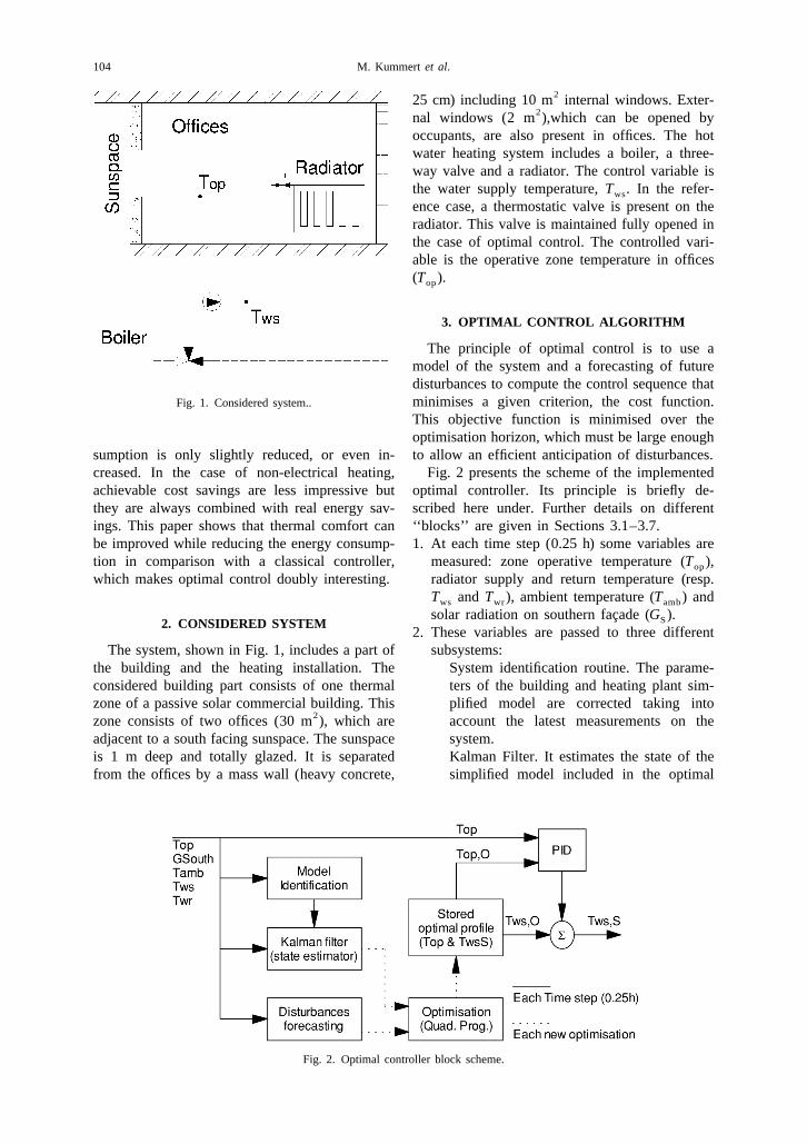
225 cm) including 10 m internal windows. Exter-2nal windows (2 m ),which can be opened by

occupants, are also present in offices. The hotwater heating system includes a boiler, a three-way valve and a radiator. The control variable isthe water supply temperature, T . In the refer-ws

ence case, a thermostatic valve is present on theradiator. This valve is maintained fully opened inthe case of optimal control. The controlled vari-able is the operative zone temperature in offices(T ).op

3. OPTIMAL CONTROL ALGORITHM

The principle of optimal control is to use amodel of the system and a forecasting of futuredisturbances to compute the control sequence thatminimises a given criterion, the cost function.Fig. 1. Considered system..

This objective function is minimised over theoptimisation horizon, which must be large enough

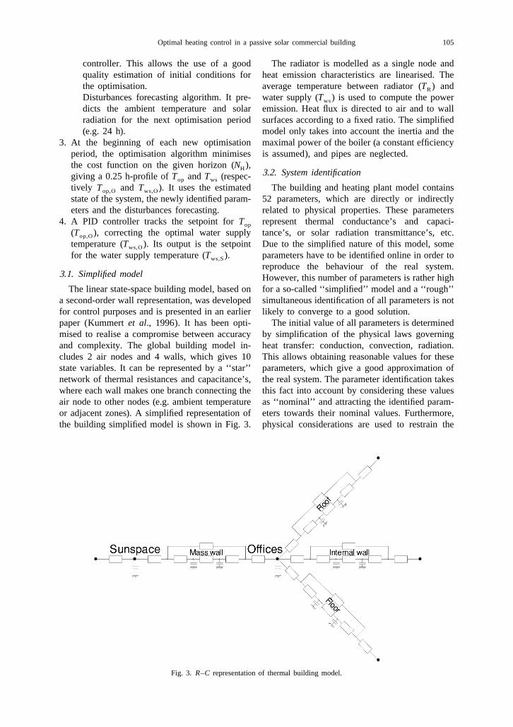
sumption is only slightly reduced, or even in- to allow an efficient anticipation of disturbances.creased. In the case of non-electrical heating, Fig. 2 presents the scheme of the implementedachievable cost savings are less impressive but optimal controller. Its principle is briefly de-they are always combined with real energy sav- scribed here under. Further details on differentings. This paper shows that thermal comfort can ‘‘blocks’’ are given in Sections 3.1–3.7.be improved while reducing the energy consump- 1. At each time step (0.25 h) some variables aretion in comparison with a classical controller, measured: zone operative temperature (T ),op

which makes optimal control doubly interesting. radiator supply and return temperature (resp.T and T ), ambient temperature (T ) andws wr amb

solar radiation on southern facade (G ).S2. CONSIDERED SYSTEM2. These variables are passed to three different

The system, shown in Fig. 1, includes a part of subsystems:the building and the heating installation. The System identification routine. The parame-considered building part consists of one thermal ters of the building and heating plant sim-zone of a passive solar commercial building. This plified model are corrected taking into

2zone consists of two offices (30 m ), which are account the latest measurements on theadjacent to a south facing sunspace. The sunspace system.is 1 m deep and totally glazed. It is separated Kalman Filter. It estimates the state of thefrom the offices by a mass wall (heavy concrete, simplified model included in the optimal

Fig. 2. Optimal controller block scheme.

Optimal heating control in a passive solar commercial building 105

controller. This allows the use of a good The radiator is modelled as a single node andquality estimation of initial conditions for heat emission characteristics are linearised. Thethe optimisation. average temperature between radiator (T ) andR

Disturbances forecasting algorithm. It pre- water supply (T ) is used to compute the powerws

dicts the ambient temperature and solar emission. Heat flux is directed to air and to wallradiation for the next optimisation period surfaces according to a fixed ratio. The simplified(e.g. 24 h). model only takes into account the inertia and the

3. At the beginning of each new optimisation maximal power of the boiler (a constant efficiencyperiod, the optimisation algorithm minimises is assumed), and pipes are neglected.the cost function on the given horizon (N ),H 3.2. System identificationgiving a 0.25 h-profile of T and T (respec-op ws

tively T and T ). It uses the estimated The building and heating plant model containsop,O ws,O

state of the system, the newly identified param- 52 parameters, which are directly or indirectlyeters and the disturbances forecasting. related to physical properties. These parameters

4. A PID controller tracks the setpoint for T represent thermal conductance’s and capaci-op

(T ), correcting the optimal water supply tance’s, or solar radiation transmittance’s, etc.op,O

temperature (T ). Its output is the setpoint Due to the simplified nature of this model, somews,O

for the water supply temperature (T ). parameters have to be identified online in order tows,S

reproduce the behaviour of the real system.3.1. Simplified model However, this number of parameters is rather high

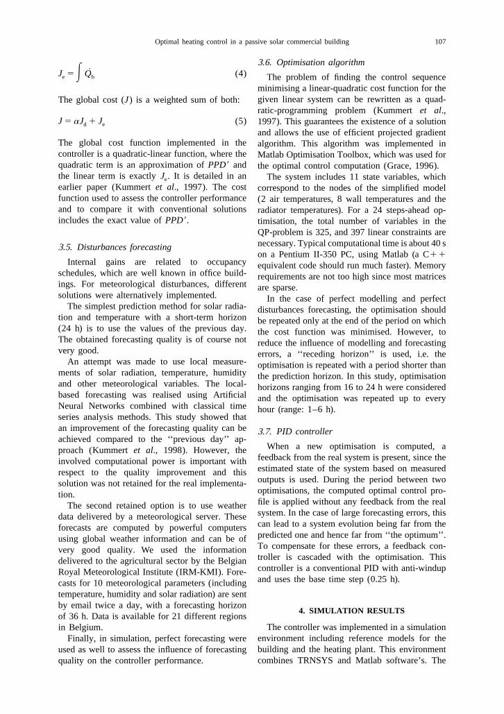
The linear state-space building model, based on for a so-called ‘‘simplified’’ model and a ‘‘rough’’a second-order wall representation, was developed simultaneous identification of all parameters is notfor control purposes and is presented in an earlier likely to converge to a good solution.paper (Kummert et al., 1996). It has been opti- The initial value of all parameters is determinedmised to realise a compromise between accuracy by simplification of the physical laws governingand complexity. The global building model in- heat transfer: conduction, convection, radiation.cludes 2 air nodes and 4 walls, which gives 10 This allows obtaining reasonable values for thesestate variables. It can be represented by a ‘‘star’’ parameters, which give a good approximation ofnetwork of thermal resistances and capacitance’s, the real system. The parameter identification takeswhere each wall makes one branch connecting the this fact into account by considering these valuesair node to other nodes (e.g. ambient temperature as ‘‘nominal’’ and attracting the identified param-or adjacent zones). A simplified representation of eters towards their nominal values. Furthermore,the building simplified model is shown in Fig. 3. physical considerations are used to restrain the

Fig. 3. R–C representation of thermal building model.


possible range of every parameter (e.g. a conduct- model must be known. These variables cannot beance must be positive). measured on a real system and the Kalman filter

The parametric identification uses a prediction is a simple and effective way to estimate themerror method. It is realised in two distinct steps: from the measured outputs.

First, the data measured over a long period (e.g. The state estimator uses the measured zone1–3 weeks) is used to identify a constant value for temperature (T ) and measured inputs and distur-op

each parameter, ‘‘attracting’’ the parameters to- bances: radiator supply and return water tempera-wards their nominal value. The minimised criter- ture (resp. T and T ), ambient conditions (Gws wr S

ion (Vl) is: and T ). The internal model of the Kalman filteramb

uses the latest parameters values obtained by theNpN2 system identification phase.2Vl 5O e (t ) 1O w G 2 1 (1)s di j R, j

i51 j51

3.4. Cost functionwith e model error on T (simulated – mea-op

sured); w weight of parameter j in the criterion;j The cost function must be an expression of theG normalised value of parameter j, defined byR, j trade-off between comfort and energy consump-

tion. The chosen indicator of thermal comfort isG 5 G /G (2)R, j j Nom, j Fanger’s PPD (Fanger, 1972), while energy costis considered to be proportional to the boilerwhere G is the nominal value for parameter j.Nom, j

energy consumption (Q ). In the discomfort cost,Secondly, the four last time steps (1 h data) are b

PPD is computed with default parameters forused to identify some parameters that are likely tonon-measured aspects (air velocity, humidity andvary with a small time constant due to a variationmetabolic activity). Furthermore, it is assumedin the real system (e.g. infiltration rate is depen-that occupants can adapt their clothing to the zonedent on windows opening) or due to simplifica-temperature. This method allows modelling ation hypothesises (e.g. incorrect evaluation ofcomfort range in which occupants are satisfied.glazing optical properties, linearisation of radia-With the chosen value for parameters, the comforttive heat fluxes).zone covers operative temperatures from 218C toIn this case, only some parameters are iden-248C. PPD is also shifted down by 5%, to give atified, the other ones being ‘‘frozen’’ to the valuesminimum value of 0. This modified PPD indexobtained during the first identification process.will be referred to as PPD9. Discomfort costThe minimised criterion is simply the predictionfunction is represented Fig. 4.error criterion (first term of Eq. (1)).

This gives, respectively for discomfort cost and3.3. State estimator energy cost (J and J ):d e

The model initial state must be estimated at thebeginning of each optimisation period. The initial J 5E PPD[%] 2 5 (3)s ddvalues of all state variables in the simplified

Fig. 4. Discomfort cost function.


3.6. Optimisation algorithm~J 5E Q (4)e b The problem of finding the control sequence

minimising a linear-quadratic cost function for thegiven linear system can be rewritten as a quad-The global cost (J) is a weighted sum of both:ratic-programming problem (Kummert et al.,

J 5 aJ 1 J (5) 1997). This guarantees the existence of a solutiond e

and allows the use of efficient projected gradientThe global cost function implemented in the algorithm. This algorithm was implemented incontroller is a quadratic-linear function, where the Matlab Optimisation Toolbox, which was used forquadratic term is an approximation of PPD9 and the optimal control computation (Grace, 1996).the linear term is exactly J . It is detailed in an The system includes 11 state variables, whiche

earlier paper (Kummert et al., 1997). The cost correspond to the nodes of the simplified modelfunction used to assess the controller performance (2 air temperatures, 8 wall temperatures and theand to compare it with conventional solutions radiator temperatures). For a 24 steps-ahead op-includes the exact value of PPD9. timisation, the total number of variables in the

QP-problem is 325, and 397 linear constraints arenecessary. Typical computational time is about 40 s3.5. Disturbances forecastingon a Pentium II-350 PC, using Matlab (a C11

Internal gains are related to occupancy equivalent code should run much faster). Memoryschedules, which are well known in office build- requirements are not too high since most matricesings. For meteorological disturbances, different are sparse.solutions were alternatively implemented. In the case of perfect modelling and perfect

The simplest prediction method for solar radia- disturbances forecasting, the optimisation shouldtion and temperature with a short-term horizon be repeated only at the end of the period on which(24 h) is to use the values of the previous day. the cost function was minimised. However, toThe obtained forecasting quality is of course not reduce the influence of modelling and forecastingvery good. errors, a ‘‘receding horizon’’ is used, i.e. the

An attempt was made to use local measure- optimisation is repeated with a period shorter thanments of solar radiation, temperature, humidity the prediction horizon. In this study, optimisationand other meteorological variables. The local- horizons ranging from 16 to 24 h were consideredbased forecasting was realised using Artificial and the optimisation was repeated up to everyNeural Networks combined with classical time hour (range: 1–6 h).series analysis methods. This study showed thatan improvement of the forecasting quality can be 3.7. PID controllerachieved compared to the ‘‘previous day’’ ap-

When a new optimisation is computed, aproach (Kummert et al., 1998). However, thefeedback from the real system is present, since theinvolved computational power is important withestimated state of the system based on measuredrespect to the quality improvement and thisoutputs is used. During the period between twosolution was not retained for the real implementa-optimisations, the computed optimal control pro-tion.file is applied without any feedback from the realThe second retained option is to use weathersystem. In the case of large forecasting errors, thisdata delivered by a meteorological server. Thesecan lead to a system evolution being far from theforecasts are computed by powerful computerspredicted one and hence far from ‘‘the optimum’’.using global weather information and can be ofTo compensate for these errors, a feedback con-very good quality. We used the informationtroller is cascaded with the optimisation. Thisdelivered to the agricultural sector by the Belgiancontroller is a conventional PID with anti-windupRoyal Meteorological Institute (IRM-KMI). Fore-and uses the base time step (0.25 h).casts for 10 meteorological parameters (including

temperature, humidity and solar radiation) are sentby email twice a day, with a forecasting horizon

4. SIMULATION RESULTSof 36 h. Data is available for 21 different regions

The controller was implemented in a simulationin Belgium.environment including reference models for theFinally, in simulation, perfect forecasting werebuilding and the heating plant. This environmentused as well to assess the influence of forecastingcombines TRNSYS and Matlab software’s. Thequality on the controller performance.


role of the real system is played by differentmodels implemented in TRNSYS. The optimalcontroller is implemented in Matlab. The com-munication between TRNSYS and Matlab isrealised by a special TRNSYS TYPE calling theMatlab Engine Library. This simulation environ-ment is described in an earlier paper (Kummert

´and Andre, 1999). These simulations tests al-lowed to tune some parameters of the controllerand to assess its performance in comparison witha conventional control strategy. All simulationsconcerned a passive solar building characterisedby an important south-facing glazed area and by ahigh thermal inertia. Some significant results arepresented here under.

4.1. Comfort /Energy trade-off

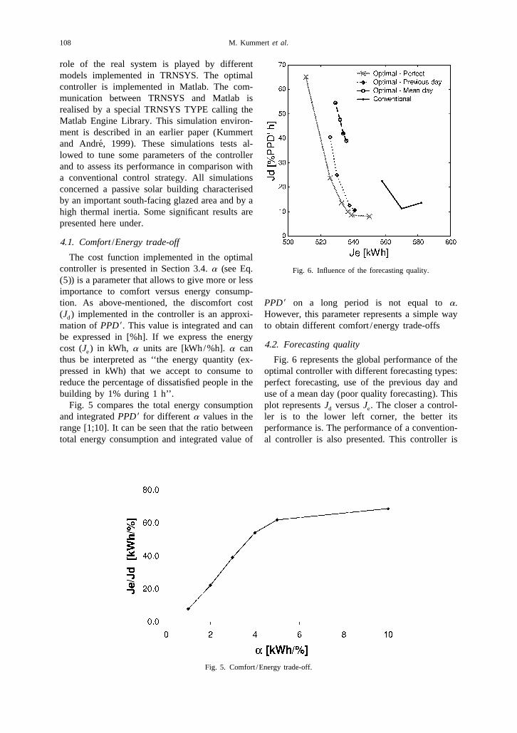
The cost function implemented in the optimalcontroller is presented in Section 3.4. a (see Eq. Fig. 6. Influence of the forecasting quality.(5)) is a parameter that allows to give more or lessimportance to comfort versus energy consump-tion. As above-mentioned, the discomfort cost PPD9 on a long period is not equal to a.(J ) implemented in the controller is an approxi- However, this parameter represents a simple wayd

mation of PPD9. This value is integrated and can to obtain different comfort /energy trade-offsbe expressed in [%h]. If we express the energy

4.2. Forecasting qualitycost (J ) in kWh, a units are [kWh/%h]. a cane

thus be interpreted as ‘‘the energy quantity (ex- Fig. 6 represents the global performance of thepressed in kWh) that we accept to consume to optimal controller with different forecasting types:reduce the percentage of dissatisfied people in the perfect forecasting, use of the previous day andbuilding by 1% during 1 h’’. use of a mean day (poor quality forecasting). This

Fig. 5 compares the total energy consumption plot represents J versus J . The closer a control-d e

and integrated PPD9 for different a values in the ler is to the lower left corner, the better itsrange [1;10]. It can be seen that the ratio between performance is. The performance of a convention-total energy consumption and integrated value of al controller is also presented. This controller is

Fig. 5. Comfort /Energy trade-off.


based on a combination of a heating curve with ‘‘day’’ curve in order to allow a quicker warm-upthermostatic valves and makes use of a simple of the building, leaving to the thermostatic valvesoptimal start algorithm (Seem et al., 1989). the role to maintain indoor temperature below

Different values of a are used (1 to 5) for each their setpoint. The night heating curve can beforecasting case. The performance decrease re- slightly underestimated since the building willsulting from the use of ‘‘previous day’’ forecast- almost never meet steady-state ‘‘night’’ condi-ing is not too important: for a discomfort about tions, but this is not often done.12, the energy consumption rises from 533 to 538,

5.1.2. Reference controller. This controllerwhich represents a 1% increase. The differencerealises a purely thermostatic control acting on theincreases for lower a values (higher part of thewater supply temperature to maintain the desiredplot). This can be explained by the greatertemperature in the reference room. The thermo-freedom left to the controller for small a values:static valves are removed in this room. A fixedachievable gains are more important in this case,schedule is used to allow a pre-heating timebut the optimal zone temperature profile is verybefore occupancy.dependent on meteo conditions. In this case, a

The main advantage of this controller, com-forecasting error has a larger influence. Thepared to the conventional one, is that it does notcomparison with the conventional controllerassume a steady-state of the building. This willshows that the optimal controller still gives aresult in the maximum usage of boiler power forbetter performance despite imperfect forecasting.pre-heating, which allows for a less conservativeIn the case of ‘‘mean day’’ forecasting, thefixed schedule, and this will effectively switch thecontroller performance is quite poor, and lowheating off during night, as long as the nightdiscomfort cost values cannot be attained.setpoint is exceeded. Combining a more efficientThis comparison shows that the quality ofnight setback and a later start of the heating, thismeteorological forecasting is an important factorcontroller can lead to significant energy savingsfor the controller but it also shows that the use ofcompared to the conventional one, without requir-the previous day seems to be a satisfying solution.ing much intelligence in the algorithm. In prac-tice, the thermostatic control is realised by a PIDalgorithm acting on Tws.5. EXPERIMENTAL RESULTS

The optimal controller was implemented in a 5.1.3. Optimal controller. This controller hasreal building on the university campus. Two been described in details in previous sections. Aoffices were selected to play the role of the mid-range comfort level (a 56–7 in Eq. (5)) wasreference zone. All system’s variable (internal, applied most of the time. Some tests were madeexternal and water temperatures, flow-rates, solar with higher values, but no significant differenceradiation) were recorded during two heating was noted. Lower comfort settings values wereseasons. The operative temperature of each room not implemented to maintain the temperature inwas measured by a special sensor presenting a an acceptable range for building occupants, whorelative sensitivity to radiation and convection considered the retained ‘‘comfort temperature’’close to the one of a human body. (218C) as ‘‘rather cold’’.

Meteorological forecasts provided by IRM5.1. Compared controllers (Royal Meteorological Institute of Belgium) were

used during half of the optimal controller testing5.1.1. Conventional controller. The im- period instead of local-based forecasting. The

plemented algorithm mimics the existing heating latter was actually reduced to the use of previouscontrol scheme in the building. The water supply day data as forecasts, as the neural networktemperature is controlled by a heating curve approach did not give satisfying results.varying according to a fixed schedule. The heatingcurve is designed to maintain 218C during day

5.2. Typical daily profilesand 158C during night (or week-ends). Thermo-static valves are placed on each radiator and set The next figures (Figs. 7–11) represent typicalby building occupants according to their prefer- profiles of the following variables: T : operativeop

ences. temperature in reference offices; T : Water sup-ws

The good practice when choosing the heating ply temperature; T : Water return temperature;wr

curve in such installations is to overestimate the Q : Radiator emission power; T : Ambientr amb


Fig. 7. Sunny days, conventional controller.

temperature; G : Solar radiation on southern ture range (21–248C) when building is occupiedsouth

facade (from 8 AM to 6 PM). The discomfort cost isGrey rectangles represent the comfort tempera- zero in this temperature range. Light grey rectan-

Fig. 8. Sunny days, reference controller.


Fig. 9. Typical Monday and Tuesday, optimal controller.

gles next to them indicate the zone where comfort T and T are represented for the referencews wr

is still very low (i.e. 0.58C below the lower limit and optimal controller because they show theand 0.58C above the upper limit). controlled variable (T ), while Q is used for thews r

Fig. 10. Cold and cloudy days, optimal controller.


Fig. 11. Sunny mid-season days, optimal controller.

conventional controller. Thermostatic valves con- temperature is already outside the comfort range,in other words when it is too late.trol the flowrate in radiators, so this power would

not be accurately represented by the temperature5.2.2. Reference controller. Fig. 8 presents twoprofile alone.

sunny mid-season days, when the reference con-troller was implemented.5.2.1. Conventional controller. Fig. 7 shows

The applied heating schedule is not too con-that important overheating can occur in the build-servative for the concerned period, which can being when the conventional controller is im-seen the first day: the desired temperature isplemented.reached just after the theoretical occupation start.The fixed heating schedule cannot be adapted

However, after this sunny day, the buildingto all conditions and is too conservative if thestructure is significantly warmer and the requiredbuilding has been submitted to high solar radia-pre-heating time is far less important during thetion during some successive days. It is the casesecond day. The temperature is at the desired

for this period: heating is started at 3AM, which islevel at occupancy start, but increases immedi-

a good compromise for this time of the year ately after and overheating occurs in the after-(February). However, the building is very warm noon.already. The thermostatic valves close quite This phenomenon is less important than for thequickly (reacting not only to the zone temperature conventional controller (for which the thermo-but also to the radiator temperature itself), but the static valve proportional band causes the heatingzone is nevertheless heated to about 218C before to stop later), but it is still present.occupants arrive. It can be seen again that the occupants open the

During the day, internal and solar gains lead to windows when the temperature reaches the upperoverheating and to discomfort. Note that overheat- comfort limit, interrupting the temperature raise,ing occurs even if the windows are open. It can be but too late.seen on the graph that the increase of temperatureis suddenly slowed down around 13:00 or 14:00, 5.2.3. Optimal controller. Fig. 9 shows tem-due to windows opening. It is also very interesting perature profiles for two typical winter daysto note that users open the windows when the (Monday and Tuesday). It can be seen that the


optimal controller starts heating at the latest Different controllers were alternatively im-moment to reach an acceptable temperature when plemented in the same building, during twooccupants are supposed to enter the building. heating seasons (1998–2000). The global per-During occupation, the heating is reduced earlier formance of different controllers cannot be com-than in the case of conventional heating (thermo- pared directly, as meteorological and user be-static valves or PID) because internal and solar haviour characteristics were different for each ofgains are anticipated. them. The performance comparison will be based

Fig. 8 shows Temperature profiles for two cold on two different techniques:and cloudy days. The first day shows an influence • consideration of ‘‘short’’ periods (2–4 weeks)of the PID correction. If the forecasted zone presenting similar weather and occupancy con-temperature is not maintained with the foreseen ditionswater supply temperature, a correction is applied • use of simulation to compute the performanceto maintain the desired zone temperature. To of controllers that were not implementedprevent unnecessary overheating, this correction is

6.1. Comparison on short periodsnot applied if the temperature lies between com-fort bounds. During this day, the foreseen tem- The first comparison concerns the conventionalperature was higher than the real one, because of and optimal controllers, for which two similaroverestimated solar radiation forecasts. The PID 2-weeks periods are considered.does not track this temperature if the real tem- Table 1 shows the summary of relevantperature lies within the comfort range, but well if meteorological parameters and of both controllersit lies outside. This can lead to oscillations in the performance during the retained period. Thewater supply temperature if the zone temperature weather conditions are representative of ratheris close to the lower comfort bound. warm and sunny mid season periods. These

The second day of Fig. 10 shows a typical ‘‘end results are obtained on relatively short periods,of day’’ profile: the radiator temperature drops but can still give a good idea of the relativesince 12 PM and the zone temperature falls just performance of both controllers.below the comfort level at the end of the occupa- The conventional controller uses a fixedtion period. This allows to save heating energy, schedule. During relatively warm periods, thisbut it is sometimes not appreciated by buildings schedule is too conservative, which leads to wasteoccupants (see the ‘‘users point of view’’ section). energy to pre-heat the building too long in

Finally, the building behaviour during relative- advance. Furthermore, this warm building is morely warm and sunny days is presented Fig. 11. This subject to overheating. This last point is stillfigure can be compared to Figs. 7 and 8. The reinforced by the proportional band of the thermo-optimal controller allows to save both energy and static valves, which reduce the power when thediscomfort in the case of high solar gains leading temperature reaches the setpoint but do not reallyto overheating. The two means that can be used to stop the heating until the temperature is aboutobtain this result are: 0.58C above this setpoint.

Delay the heating start to reach the comfort In this kind of situation, the optimal controllertemperature at the latest moment or even just after is able to reduce the energy consumption whiledue time, to maintain a colder building structure. reducing the discomfort. Energy savings on the

Maintain the temperature slightly below the considered period reach 13%, for a significantlycomfort range during the early morning in orderto decrease the maximum temperature reached inthe afternoon.

Table 1. Weather, comfort and energy parameters, optimaland conventional controllers, sunny mid season period

6. PERFORMANCE COMPARISON Conventional Optimal

T [8C] Min 2.0 3.5The available experimental facility did not amb

Max 18.7 17.2allow the simultaneous implementation of differ-Avg 10.0 9.3

2ent controllers. Furthermore, it would have been G [W/m ] Avg 67 62S

J [%PPD9] Max 3.8 2.4almost impossible to obtain a similar user be- d

Avg 0.25 0.07haviour in two different reference rooms, andPMV 9 [–] Min 20.13 20.34

users have a strong influence on the thermal Max 0.43 0Avg 0.04 20.02behaviour of the building by opening or closing

P [kW] Avg 0.175 0.152heatthe windows.


reduced discomfort (‘‘optimal’’ discomfort cost is parison between different controllers implemented28% from ‘‘conventional’’ cost). on one single building.

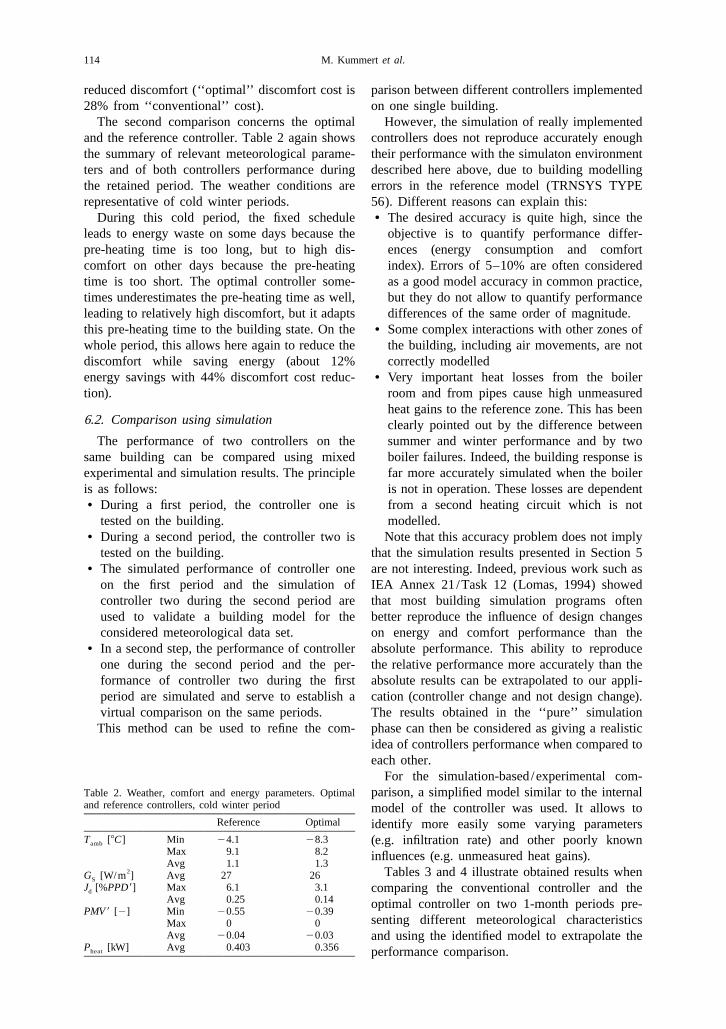
The second comparison concerns the optimal However, the simulation of really implementedand the reference controller. Table 2 again shows controllers does not reproduce accurately enoughthe summary of relevant meteorological parame- their performance with the simulaton environmentters and of both controllers performance during described here above, due to building modellingthe retained period. The weather conditions are errors in the reference model (TRNSYS TYPErepresentative of cold winter periods. 56). Different reasons can explain this:

During this cold period, the fixed schedule • The desired accuracy is quite high, since theleads to energy waste on some days because the objective is to quantify performance differ-pre-heating time is too long, but to high dis- ences (energy consumption and comfortcomfort on other days because the pre-heating index). Errors of 5–10% are often consideredtime is too short. The optimal controller some- as a good model accuracy in common practice,times underestimates the pre-heating time as well, but they do not allow to quantify performanceleading to relatively high discomfort, but it adapts differences of the same order of magnitude.this pre-heating time to the building state. On the • Some complex interactions with other zones ofwhole period, this allows here again to reduce the the building, including air movements, are notdiscomfort while saving energy (about 12% correctly modelledenergy savings with 44% discomfort cost reduc- • Very important heat losses from the boilertion). room and from pipes cause high unmeasured

heat gains to the reference zone. This has been6.2. Comparison using simulation clearly pointed out by the difference between

The performance of two controllers on the summer and winter performance and by twosame building can be compared using mixed boiler failures. Indeed, the building response isexperimental and simulation results. The principle far more accurately simulated when the boileris as follows: is not in operation. These losses are dependent• During a first period, the controller one is from a second heating circuit which is not

tested on the building. modelled.• During a second period, the controller two is Note that this accuracy problem does not imply

tested on the building. that the simulation results presented in Section 5• The simulated performance of controller one are not interesting. Indeed, previous work such as

on the first period and the simulation of IEA Annex 21/Task 12 (Lomas, 1994) showedcontroller two during the second period are that most building simulation programs oftenused to validate a building model for the better reproduce the influence of design changesconsidered meteorological data set. on energy and comfort performance than the

• In a second step, the performance of controller absolute performance. This ability to reproduceone during the second period and the per- the relative performance more accurately than theformance of controller two during the first absolute results can be extrapolated to our appli-period are simulated and serve to establish a cation (controller change and not design change).virtual comparison on the same periods. The results obtained in the ‘‘pure’’ simulationThis method can be used to refine the com- phase can then be considered as giving a realistic

idea of controllers performance when compared toeach other.

For the simulation-based/experimental com-Table 2. Weather, comfort and energy parameters. Optimal parison, a simplified model similar to the internaland reference controllers, cold winter period model of the controller was used. It allows to

Reference Optimal identify more easily some varying parametersT [8C] Min 24.1 28.3 (e.g. infiltration rate) and other poorly knownamb

Max 9.1 8.2 influences (e.g. unmeasured heat gains).Avg 1.1 1.3

2 Tables 3 and 4 illustrate obtained results whenG [W/m ] Avg 27 26S

J [%PPD9] Max 6.1 3.1 comparing the conventional controller and thed

Avg 0.25 0.14 optimal controller on two 1-month periods pre-PMV 9 [2] Min 20.55 20.39

senting different meteorological characteristicsMax 0 0Avg 20.04 20.03 and using the identified model to extrapolate the

P [kW] Avg 0.403 0.356heat performance comparison.


Table 3. Weather, comfort and energy parameters. Period 1

Conventional Conventional Optimalmeasured simulated simulated

T [8C] 21.4 21.4 21.4amb min

T [8C] 18.7 18.7 18.7amb max

T [8C] 7.0 7.0 7.0amb avg2G [W/m ] 111 111 111south avg

J [%PPD9] 13.0 10.2 5.4d max

J [%PPD9 h] 280.5 262.6 215.0d tot

J [kWh] 130.5 135.0 111.6e tot

The first part of each table sums up the However, the two regular occupants of referencemeteorological parameters of the considered offices were given survey forms where they couldperiod. Comfort and energy parameters are given: write their complaints when they felt uncomfort-

18 as measured on the real building (with able. They were also surveyed on a regular basisconventional controller for period 1, with to give their opinion on the thermal and generaloptimal controller for period 2) comfort in the building. Some information can be28 as simulated for the controller that was gained from these surveys and from the fewreally applied (model validation) complaints that occurred. Note that these occup-38 as simulated for the other controller ants were not at all involved in the project nor

The results show a very good agreement between working in the field of building energy manage-simulation and experiments: the energy perform- ment.ance is reproduced within 3.5%. The larger error The first conclusion of this small survey is thaton the discomfort cost (6% on total, 27% on the comfort feeling is not always directly relatedmaximum value for 0.25 h) is due to the non- to the temperature that is measured by the control-linear shape of the cost function, which amplifies ler. Many objective and subjective factors canthe error on operative temperature (see Fig. 2). have an influence: humidity, draughts, occupants

The comparison shows that energy savings of mental /physical state, . . .20% can be achieved during the first period In this respect, a controller achieving perfect(sunny mid season) while improving the thermal thermal comfort for all occupants is not realistic.comfort by 18%. During the cold period 2, energy However, some typical user behaviours couldsavings of 7% can be achieved with a maintained be considered in the development of a commercialthermal comfort (small increase of discomfort: controller:2%). • If building occupants feel uncomfortable, their

Simulations on the entire heating season show first reaction is to verify that the radiators areimportant energy savings (15–20%) for an im- cold /warm according to what they desire. It isproved thermal comfort. Furthermore, energy also very often the case that they verify if thesavings in the range of 10% can be achieved as radiators are warm when they arrive in thewell compared to the ‘‘reference controller’’, with building on a cold winter morning. In thisa similar thermal comfort. respect, the optimal controller was appreciated

because the heating is started as late as pos-6.3. User’s point of view sible and the water temperature is very often

A real user survey about the comfort in the test high when the occupants arrive.building was out of the scope of this work. • On the other hand, it happened quite often that

Table 4. Weather, comfort and energy parameters. Period 2

Optimal Optimal Conventionalmeasured simulated simulated

T [8C] 27.3 27.3 27.3amb min

T [8C] 17.2 17.2 17.2amb max

T [8C] 4.6 4.6 4.6amb avg2G [W/m ] 51 51 51south avg

J [%PPD9] 6.7 4.9 3.02d max

J [%PPD9 h] 199.5 194.2 190.1d tot

J [kWh] 190.5 196.6 211.2e tot


Acknowledgements—This research work was partly funded bythe occupants were feeling cold on a cloudythe European Commission, in the framework of the non-

afternoon and did not appreciate the fact that nuclear energy programme JOULE III (Contract JOE3-CT97-0076).radiators were cool. With a conventional heat-

The authors also wish to thank the Belgian Royaling curve control associated with thermostaticMeteorological Institute (IRM-KMI) for providing weather

valves, they always have the possibility to forecasting data.increase the radiator temperature and the lackof such a possibility was probably the major

REFERENCESdisadvantage of the optimal controller. The´ Ándre Ph. and Nicolas J. (1992) Application de la theorie descomfort temperature setting does not play

` ` ˆ ` ´systemes a la thermique du batiment. Problemes de modeli-exactly the same role, as the real desire of the ˆ ´ ´sation, d’identification, de controle. Revue Generale deoccupants often is to feel the warmth from the Thermique 371, 600–615.

Braun J. E. (1990) Reducing energy cost and peak electricalradiator rather than to have a warmer office.demand through optimal control of building thermal storage.Concerning the overheating problem, the opti- ASHRAE Trans. 96(2), 876–888.

mal controller showed a very good behaviour. European Commission (1999). Energy, environment and sus-tainable development. Programme for Research, TechnologyMoreover, simulation results confirm that thisDevelopment and Demonstration under the Fifth Framework

controller could be suitable even during very Programme. Available on http: / /www.cordis.lu / fp5 /src / t-warm mid-season periods (when no heating is 4.htm.

Fanger P. O. (1972). Thermal comfort analysis and applicationreally needed), while the conventional controllerin environmental design, McGraw Hill.

would probably always heat the building in the Fulcheri L., Neirac F. P., Le Mouel A. and Fabron C. (1994)ˆ ´morning. The need for user adjustment of the Chauffage des batiments. Intermittence et lois de regulation

´ én boucle ouverte. Revue Generale de Thermique 387,heating curve is completely suppressed.181–189.

Grace A. (1996). Optimisation toolbox for use with Matlab 5.The MathWorks Inc, Natick MA.

Keeney K. and Braun J.E. (1996). A simplified method fordetermining optimal cooling control strategies for thermalstorage in building mass. HVAC&R Research, 2(1).7. CONCLUSIONS

´Kummert M., Andre Ph. and Nicolas J. (1996) Developmentof simplified models for solar buildings optimal control. InExperiments on a passive solar commercialProceedings of ISES Eurosun 96 Congress, Freiburg,

building have confirmed the simulation-based Germany.´study and show that the optimal controller can Kummert M., Andre Ph. and Nicolas J. (1997) Optimised

thermal zone controller for integration within a Buildingachieve significant energy savings compared toEnergy Management System. In Proceedings of CLIMA

conventional controller with thermostatic valves 2000 conference. (CD-ROM), Brussels.ánd also compared to a perfect thermostatic Kummert M., Andre Ph., Guiot J. and Nicolas J. (1998)

Short-term weather forecasting for solar buildings optimalcontrol, while maintaining or improving the ther-control: an application of neural networks. In Proceedings

mal comfort. Furthermore, choice is given to of EUFIT 98 congress, 7 –10 Sept., Aachen, Germany, Volbuilding users to privilege either the comfort or 2, Zimmermann H. J. (Ed.), pp. 868–872, Verlag, Mainz,

Aachen.energy savings thanks to a simple parameter.´Kummert M. and Andre Ph. (1999) Building and HVAC

Obtained energy savings for a maintained or optimal control simulation. Application to an office build-improved thermal comfort are about 9%, which ing. In Proceedings of the 3rd Symposium on Heating,

Ventilation and Air Conditioning (ISHVAC 99) conference,fulfills the objective mentioned in the ‘‘Energy,17 –20 Nov., Shenzen, China,II, pp. 857–868, Tsinghua

Environment and sustainable development’’ work University & Hong Kong Polytechnical University.programme of the EC Fifth Framework Pro- Lomas, K. J (Ed.). (1994). Empirical validation of thermal

building simulation programs using test room data. IEAgramme (European Commission, 1999).Task 12 & Annex 21 Final report, International Energy

Practical limitations have also been enlighted, Agency.mainly concerning the required computational Rosset M. M. and Benard C. (1986) Optimisation de la

`conduite du chauffage d’appoint d’un habitat solaire a gainpower and the a priori knowledge which is´ ´direct. Revue Generale de Thermique 291, 145–159.

necessary to give suitable initial values for the Seem J. E., Armstrong P. R. and Hancock C. E. (1989)parameters of the internal building model. These Algorithms for predicting recovery time from night setback.

ASHRAE Trans. 95(2), 439–446.aspects have to be considered carefully in order toWinn R. C. and Winn C. B. (1985) Optimal control for

make this algorithm suitable for commercial auxiliary heating of passive-solar-heated buildings. Solarapplications. Energy 35(5), 419–442.

optimal heating control in a passive solar … · used to identify some parameters that are likely...

Documents