M. A. Kutay and H. M. Ozaktas Vol. 15, No. 4 /April 1998 /J. Opt. Soc. Am. A 825

Optimal image restoration with the fractionalFourier transform

M. Alper Kutay and Haldun M. Ozaktas

Department of Electrical Engineering, Bilkent University, 06533 Bilkent, Ankara, Turkey

Received August 29, 1997; accepted September 29, 1997; revised manuscript received November 7, 1997

The classical Wiener filter, which can be implemented in O(N log N) time, is suited best for space-invariantdegradation models and space-invariant signal and noise characteristics. For space-varying degradations andnonstationary processes, however, the optimal linear estimate requires O(N2) time for implementation. Op-timal filtering in fractional Fourier domains permits reduction of the error compared with ordinary Fourierdomain Wiener filtering for certain types of degradation and noise while requiring only O(N log N) implemen-tation time. The amount of reduction in error depends on the signal and noise statistics as well as on thedegradation model. The largest improvements are typically obtained for chirplike degradations and noise, butother types of degradation and noise may also benefit substantially from the method (e.g., nonconstant velocitymotion blur and degradation by inhomegeneous atmospheric turbulence). In any event, these reductions areachieved at no additional cost. © 1998 Optical Society of America [S0740-3232(98)00604-8]

OCIS codes: 070.2590, 100.3020.

1. INTRODUCTIONRestoration of degraded or distorted and noisy images is abasic problem in image and optical processing, with manyapplications. The objective is to reduce or eliminate thedegradations or distortions that are introduced typicallyby the transmission channel and the sensing environ-ment. A variety of approaches to degradation removalhave been proposed (for instance, see Ref. 1). The effec-tiveness of these methods depends on the observationmodel and the design criteria used as well as on the priorknowledge available about the desired signal, degrada-tion process, and noise. One of the most popular obser-vation models is of the form

o 5 H~f ! 1 n, (1)

where o is the observed signal, f is the signal we wish torecover, n is an additive and possibly nonstationary noisesignal, and H is the system representing undesired lineartime-varying distortion. A frequently used design crite-rion is the mean-square error (MSE), and we usually con-sider a linear estimation of the form

f 5 G ~o!. (2)

Then the problem is to find the operator G opt that mini-mizes the MSE.

The well-known classical Wiener filtering presents asolution to the above problem under the assumption thatthe signals involved are stationary and H is a time-invariant system. This filter turns out to be a time-invariant one that corresponds to a multiplicative filter inthe Fourier domain and thus can be implemented inO(N log N) time, where N is the space–bandwidth prod-uct of the images, i.e., the number of pixels in the image.The general solution when the above assumptions do nothold is also known.2 However, since the resulting linearoperator is not time-invariant and thus cannot be ex-pressed as a convolution, obtaining this most general lin-

0740-3232/98/040825-09$15.00 ©

ear estimate requires computational time of O(N2) as op-posed to O(N log N) for the time-invariant case. We canstill seek the optimal ordinary Fourier domain Wiener fil-ter, but this filter is not as satisfactory as the general lin-ear estimator.

The possibility of realizing various time-varying opera-tions by filtering in fractional Fourier domains was sug-gested in Ref. 3. An exact analytical solution for the op-timal filtering problem (analogous to the Wiener filteringproblem) in fractional domains for one-dimensional (1D)signals was given in Ref. 4. Filtering in a fractional Fou-rier domain can be implemented as efficiently as filteringin the conventional Fourier domain, since the fractionalFourier transformation has a fast digital algorithm4,5 andcan also be optically realized much like the usual Fouriertransform.6–10 Thus any improvement obtained with thefractional Fourier transformation comes at no additionalcost.

In this paper the concept of filtering in fractional Fou-rier domains is applied to the problem of estimating im-ages [or other two-dimensional (2D) signals] with space-varying statistics in the presence of space-varyingdegradation and noise. Expressions for the 2D optimalfilter function in fractional domains will be given fortransform domains characterized by the two-order pa-rameters of the 2D fractional Fourier transform. Thenwe will seek the optimal values of these parameters, thusachieving the smallest possible error with the proposedmethod. Since the class of fractional Fourier domain fil-ters is a subclass of the class of all linear operators, forthe arbitrary time-varying degradation model the MSEobtained by the proposed method will still not be as smallas the one obtained by the general linear estimator.However, the class of proposed filters is a much broaderclass than ordinary Fourier domain filters, and it is pos-sible to obtain smaller MSE’s in comparison with ordi-nary Fourier domain filters. It will be shown in the ex-

1998 Optical Society of America

826 J. Opt. Soc. Am. A/Vol. 15, No. 4 /April 1998 M. A. Kutay and H. M. Ozaktas

amples that the method is very effective, especially whenthe noise and degradations are of chirped nature. It willalso be shown that substantial reduction in error can beachieved for other interesting types of degradation andnoise that are encountered in practice. We expect theproposed method to be applicable to other degradation-and-noise models not discussed in this paper.

2. TWO-DIMENSIONAL FRACTIONALFOURIER TRANSFORMATIONIn this section we give the definition of the 2D fractionalFourier transformation. The fractional Fourier trans-form is the generalization of the ordinary Fouriertransform.6,11–14 The fractional Fourier transform hasbeen found to have several applications in fields includingthe solution of differential equations, quantum mechan-ics, diffraction theory and optical propagation, optical sys-tems and signal processing, swept-frequency filters,space-variant filtering and multiplexing, and the study oftime- and space-frequency distributions.3,6,9,12–24 Itsanalog optical implementation was discussed in Refs. 6, 9,and 15, and its digital implementation was discussed inRef. 5.

One of the most important properties of the fractionalFourier transform is its relation to time- and space-frequency representations.9,14,25,26 This property statesthat the fractional Fourier transformation corresponds toa rotation in the time- and space-frequency plane for cer-tain members of Cohen’s class. It leads us to the conceptof fractional Fourier domains27 and also suggests a way ofperforming certain time-varying operations by employingthe fractional Fourier transform.3,4

The ath-order fractional Fourier transform of a 1Dfunction f(x) may be defined for 0 , uau , 2 as

@F a~f !#~x ! 5 fa~x !

5 E Ba~x, x8!f~x8!dx8,

Ba~x, x8! 5 Af exp@ip~x2 cot f

2 2xx8 csc f 1 x82 cot f!#,

Af 5 ~ usin fu!21/2 exp@ip sgn~sin f!/4 2 if/2#,(3)

where f [ ap/2. The kernel Ba(x, x8) approaches d (x2 x8) or d (x 1 x8) when a approaches 0 or 62, respec-tively. The definition is easily extended outside the in-terval @22, 2# since F 4 is the identity operation.

A direct generalization of the above definition to 2D sig-nals is given by

fax, ay~x, y ! 5 $F ax, ayf %~x, y !

5 EE Bax, ay~x, y; x8, y8!f~x8, y8!dx8dy8,

Bax, ay~x, y; x8, y8!

5 Bax~x, x8!Bay

~y, y8!.

The 2D transform kernel is the product of two 1D kernelsas in the case of the ordinary Fourier transform, but we

allow different orders ax and ay for the two coordinates.Efficient analog optical implementations of such anamor-phic 2D transforms has been demonstrated.10,28,29 Digi-tal computation is also possible with direct modificationsto the algorithm developed for 1D signals5 since 2D trans-formation is defined as separable so that the associatedkernel is just the product of two 1D kernels.

3. FILTERING IN FRACTIONAL FOURIERDOMAINSIn this section the mathematical definition of the problemis given, and our approach to its solution is formulated.The solution for the case of a linear space-invariant deg-radation model with stationary processes is the well-known optimal Wiener filter, which can be implementedefficiently with the fast Fourier transform. For space-varying degradation models and nonstationary signalsand noise, the optimal recovery operator is also knownbut in general requires O(N2) time for implementation,where N is the space–bandwidth product of the signal,i.e., the number of pixels in the image.

First, we briefly review the general linear filteringproblem. Our signal observation model can be written as

o~x, y ! 5 EE h~x, y; x8, y8!f~x8, y8!dx8dy8 1 n~x, y !,

(4)

where h(x, y; x8, y8) is the kernel of the degradationmodel and n(x, y) is the additive noise term. (All inte-grals are from minus infinity to plus infinity unless oth-erwise stated.) We assume that as prior knowledge weknow the correlation functions Rff (x, y; x8, y8)5 E@ f(x, y)f * (x8, y8)#, Rnn(x, y; x8, y8) 5 E@n(x, y)

3 n* (x8, y8)# of the input signal (desired signal) f andthe noise. We further assume that the noise is indepen-dent of the input f and is zero mean, i.e., E@n(x, y)#5 0 for all x and y, and that we know the degradation

model. Under these assumptions we can also find thecross-correlation function Rfo(x, y; x8, y8) 5 E@ f(x, y)3 o* (x8, y8)# of the processes f and o and the correlationfunction Roo(x, y; x8, y8) 5 E@o(x, y)o* (x8, y8)# by us-ing Eq. (4).

Consider the most general linear estimate of the form

f~x, y ! 5 EE g~x, y; x8, y8!f~x8, y8!dx8dy8. (5)

Our design criteria is the MSE, which is defined as

se2 5 E~ if 2 f i2!, (6)

where E( • ) denotes the expectation operator and i•i de-notes the norm

if i2 5 EE u f~x, y !u2dxdy. (7)

This definition [Eq. (6)] of the MSE with the norm definedin Eq. (7) is appropriate for nonstationary signals whosefunctional representations are square integrable (of finiteenergy). [For stationary processes, the MSE may bedefined as the expected value of the magnitude squaredof the difference term.2] The problem is then to findthe optimal recovery operator kernel, denoted by

M. A. Kutay and H. M. Ozaktas Vol. 15, No. 4 /April 1998 /J. Opt. Soc. Am. A 827

Fig. 1. (a) Original (desired) plane image; (b) corrupted image (SNR ' 1), (c) estimated image obtained by filtering in optimum frac-tional Fourier domain (ax 5 0.4, ay 5 20.6), (d) image restored by filtering in ordinary Fourier domain.

gopt(x, y; x8, y8), which minimizes the MSE. The solu-tion to this problem, with the linear estimate defined inEq. (5), is known, and gopt(x, y; x8, y8) is the kernel thatsatisfies the following equation2:

Rfo~x, y; x8, y8!

5 EE gopt~x, y; x9, y9!Roo~x9, y9; x8, y8!dx9dy9

(8)

Equation (8) can be solved numerically to yield the kernelof the optimal linear recovery operator. However, appli-cation of this estimation operator [see Eq. (5)] on a givendistorted and noisy signal would require O(N2) time,where N is the space–bandwidth product of the signals(the number of pixels for images). In this paper we re-strict our estimate so that it corresponds to a multiplica-tion by a filter function in the fractional Fourier domain.This estimate can be written as

f~x, y ! 5 F 2ax, 2ay$m~x, y !F ax ,ay@o~x, y !#%, (9)

where F ax ,ay is the 2D fractional Fourier transformationoperator with different-order parameters for eachdimension10 and m(x, y) is the multiplicative filter. Ac-cording to Eq. (9), we first take the 2D fractional Fouriertransform of the observed signal o(x, y) with orders axand ay and then multiply the transformed signal with thefilter m(x, y) and take the inverse 2D fractional Fouriertransform of the resulting signal. Thus the filter m(x, y)has been applied in the fractional Fourier domain of or-ders ax and ay . We note that for ax 5 ay 5 1 this esti-mate corresponds to filtering in the conventional Fourierdomain. With this form of estimation operator the mini-mization problem considered in this paper is to find theoptimal filter function, denoted by mopt(x, y), that mini-mizes the MSE defined in Eq. (6) with the estimatef(x, y) given by Eq. (9). The class of fractional Fourierdomain filters is a subclass of the class of all linear opera-tors, so the linear filter we find is not the most optimalamong all linear operators. However, it is a much

828 J. Opt. Soc. Am. A/Vol. 15, No. 4 /April 1998 M. A. Kutay and H. M. Ozaktas

broader class than (time-invariant) Fourier domain fil-ters, and in many problems involving time-varying degra-dation models and nonstationary processes, it is possibleto obtain smaller MSE’s in comparison with filtering inthe conventional Fourier domain. This reduction in MSEcomes at no additional cost, because the resulting filtercan be implemented digitally in O(N log N) time just likethe ordinary Fourier transform,5 or can be implementedoptically with the same kind of hardware as that of theordinary Fourier transform.6–9

We finally note that although beyond the scope of thepresent paper, various extensions and refinements of theclassical filtering problem (for instance, see Refs. 34–36and the references therein) can also be applied to the frac-tional Fourier domain filtering problem that we have con-sidered.

4. OPTIMAL FRACTIONAL FOURIERDOMAIN FILTERThe solutions of the 2D and 1D problems are similar.Our estimate is given by

which is nothing but the well-known orthogonalitycondition.30,31 The above equation states that the bestlinear MSE fax, ay

(x, y) is an orthogonal projection of thesignal fax, ay

(x, y) onto the space of observations.The optimum filter function mopt( • , • ) can be solved

from Eq. (11) by use of the definition of fax, ay(x, y),

mopt~x, y ! 5

Rfax, ay,oax, ay

~x, y; x, y !

Roax, ay,oax, ay

~x, y; x, y !,

where

Rfax, ay,oax, ay

~x, y; x8, y8!, Roax, ay,oax, ay

~x, y; x8, y8!

are the correlation functions in the transform domain(ax , ay). These correlation functions can easily be cal-culated from the correlation functions in the spatial do-main so that the filter function is given by

f~x, y ! 5 F 2ax, 2ay$m~x, y !F ax, ay@o~x, y !#%,

5 EE B2ax, 2ay~x, y; x9, y9!m~x9, y9!

3 EE Bax, ay~x9, y9; x8, y8!o~x8, y8!

3 dx8dy8dx9dy9, (10)

and the error is

se2 5 E~ if 2 f i2!

5 E(i f~x, y ! 2 F 2ax,2ay$m~x, y !F ax, ay@o~x, y !#%i2).

Since the 2D fractional Fourier transformation is unitary,this MSE is equal to the error in the transform domain:

se2 5 E~ ifax, ay

2 fax, ayi2!

5 E@ ifax, ay~x, y ! 2 m~x, y !oax, ay

~x, y !i2#.

For particular values of ax and ay , the optimal filter func-tion that minimizes the above error can be shown to sat-isfy the following equation:

E$@ fax, ay~x, y ! 2 fax, ay

~x, y !#oax, ay* ~x, y !% 5 0, (11)

mopt~x, y ! 5EEEE Bax, ay

~x, y; x8, y8!B2ax, 2ay~x, y; x9, y9!Rf,o~x8, y8; x9, y9!dx8dy8dx9dy9

EEEE Bax, ay~x, y; x8, y8!B2ax, 2ay

~x, y; x9, y9!Ro,o~x8, y8; x9, y9!dx8dy8dx9dy9

. (12)

Fig. 2. (a) MSE versus ay for ax 5 0.4, (b) MSE versus ax foray 5 20.6.

M. A. Kutay and H. M. Ozaktas Vol. 15, No. 4 /April 1998 /J. Opt. Soc. Am. A 829

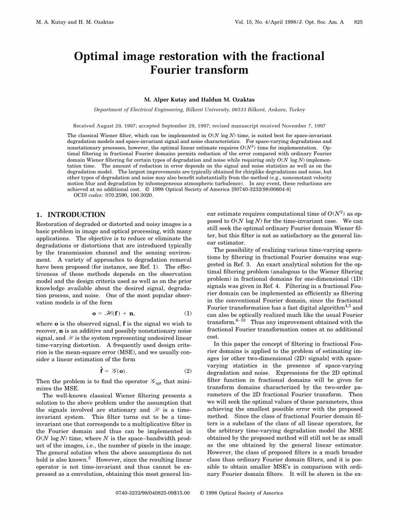
Fig. 3. (a) Original (desired) plane image, (b) corrupted image (SNR ' 0.1), (c) estimated image obtained by filtering in optimum frac-tional Fourier domain (ax 5 0.4, ay 5 20.6), (d) image restored by filtering in ordinary Fourier domain.

Equation (12) provides us the optimal multiplicative fil-ter function in the fractional domain defined by the pa-rameters ax, ay . To find the optimal values of ax anday—that is, the domain in which the smallest error isobtained—we plug the optimum filter function into theMSE expression,

se,o2 5 E H EE @ fax, ay

~x, y ! 2 fax ,ay~x, y !#

3 @fax, ay~x, y ! 2 fax, ay

~x, y !#* dxdyJ5 E $Rfax, ay

,fax ,ay~x, y; x, y ! 2 2 Re@mopt* ~x, y !

3 Rfax, ay,oax ,ay

~x, y; x, y !#

1 umopt~x, y !u2Roax, ay,oax, ay

~x, y; x, y !%dxdy,

(13)

and then choose the values of ax P @21 1# and ayP @21 1# that minimize se,o

2. (Note that MSE is peri-

odic with respect to ax and ay with period 2.) These val-ues may be found analytically in certain special cases.But these cases are exceptional. In general, we can findthe optimal values of ax and ay numerically by simply cal-culating the MSE for sufficiently closely spaced discretevalues of ax and ay (for example, with a step size of 0.1)and choosing the values that minimize the MSE. We canalso find the optimal values by employing a standard mul-tivariate optimization routine.32

Overall, the procedure can be outlined as follows:Given the autocorrelation functions of the input (f ) andnoise (n) processes, along with the degradation (H ), wecan find the correlation function between the input andoutput (o) processes and the autocorrelation function ofthe output process. Then, using these, we can find theoptimal filter function in the fractional domain character-ized by ax and ay by using Eq. (12). The optimal choicesof ax and ay are then those that minimize Eq. (13). Oncethese are determined for the given signal and noise sta-tistics and for distortion model, implementation of thefractional Fourier domain filter requires O(N log N) timefor an image with N pixels. It is important to emphasize

830 J. Opt. Soc. Am. A/Vol. 15, No. 4 /April 1998 M. A. Kutay and H. M. Ozaktas

that both the digital computation of the fractional Fouriertransform and its optical implementation are nearly as ef-ficient as the ordinary Fourier transform, so that the im-provements in performance come at essentially no cost.

5. EXAMPLESIn this section we apply our method to degraded images toillustrate the applications and performance of fractionalFourier domain filtering. In the first two examples weapply the method to images corrupted by chirplike noisesand show that the method is very effective and permitssignificant reduction in error in comparison with ordinaryFourier domain filtering for this kind of degradation.The last two examples show the performance of themethod for other types of degradation, particularly fortwo different space-varying blur models with additivewhite Gaussian noise. The reduction is less spectacularfor these examples.

Figure 1(a) shows the original image used. In Fig. 1(b)this image has been corrupted by the presence of twochirp waveforms with amplitudes selected so that thenoise energy is comparable with that of the image, mak-

ing the signal-to-noise ratio approximately one. The op-timally estimated image is shown in Fig. 1(c), for whichthe optimal-order parameters are found to be ax 5 0.4and ay 5 20.6. The minimum MSE is ;0.003 [in thissection, MSE’s are normalized by the energy of the origi-nal image E(i f i2).] For comparison, we display in Fig.1(d) the result of optimal restoration by ordinary Fourierdomain filtering (corresponding to the order parametersax 5 ay 5 1), which is less satisfactory, with MSE equalto 0.035.

We plot the profiles of the MSE along the individual or-der parameters (ax and ay) around the optimal point inFigs. 2(a) and 2(b). (We recall that MSE is periodic withrespect to the parameters ax and ay with period 2.) Theseplots show the behavior of the MSE around the optimalpoint where minimum MSE is achieved.

The above example is repeated with a signal-to-noiseratio '0.1. The corresponding images are presented inFig. 3. The benefit obtained by use of fractional Fourierdomain filtering (MSE 0.006) instead of ordinary Fourierdomain filtering (MSE 0.10) is much greater for this valueof signal-to-noise ratio.

In the following two examples we apply the method to

Fig. 4. (a) Original (desired) plane image, (b) degraded image, (c) estimated image obtained by filtering in optimum fractional Fourierdomain (ax 5 0.7, ay 5 0.8), (d) image restored by filtering in ordinary Fourier domain.

M. A. Kutay and H. M. Ozaktas Vol. 15, No. 4 /April 1998 /J. Opt. Soc. Am. A 831

Fig. 5. (a) Original (desired) plane image, (b) degraded image, (c) estimated image obtained by filtering in optimum fractional Fourierdomain (ax 5 0.4, ay 5 0.7), (d) image restored by filtering in ordinary Fourier domain.

images degraded with different space-varying blur mod-els together with an additive white Gaussian noise.These examples illustrate the performance of the methodfor degradation and noise that are not of a chirped nature.

In this example we consider nonconstant-velocity mo-tion blur. This blur corresponds to the degradation thatis the result of accelerated linear motion (in which veloc-ity is increasing linearly) between the object and the cam-era during exposure. [We should note that in the case ofconstant-velocity motion the degradation is time-invariant so that the optimal filtering domain turns out tobe the ordinary Fourier domain (ax 5 ay 5 1)]. For thistype of degradation the kernel [see Eq. (4)] is given by

h~x, y; x8, y8! 51

ax 1 a0rectS x 2 x8

ax 1 a02

12 D d~ y 2 y8!,

where a and a0 are the parameters of the distortionmodel and correspond to acceleration and initial velocity,respectively. The additive noise is white Gaussian noisewhose energy is equal to one fourth of the signal energy

(input SNR of 4). Figure 4(a) shows the original (desired)image, and Fig. 4(b) shows the distorted image (a5 0.01 and a0 5 0.3). The optimally estimated image isshown in Fig. 4(c), for which the optimal order param-eters are found to be ax 5 0.7 and ay 5 0.8. The mini-mum MSE is '0.0097. For comparison we have dis-played in Fig. 4(d) the result of optimal restoration usingordinary Fourier domain filtering (corresponding to theorder parameters ax 5 ay 5 1), which is less satisfactory,with a MSE equal to 0.0382.

In the last example we consider degradation that cor-responds to space-varying atmospheric turbulence. Thisdegradation is the result of inhomogeneous statisticalproperties of the turbulent media33 and occurs when animage covers several isoplanatic patches (regions wherestatistical properties of the turbulent media can be takento be constant). The kernel of the degradation is given by

h~x, y; x8, y8! 5 exp$2pa2~x, y !

3 @~x 2 x8!2 1 ~ y 2 y8!2#%,

832 J. Opt. Soc. Am. A/Vol. 15, No. 4 /April 1998 M. A. Kutay and H. M. Ozaktas

where a(x, y) is a function of x and y, which makes thedegradation space varying. In our example, a(x, y)5 a0 1 b(x, y), where b(x, y) represents the fluctua-tion around a0 (50.1) and is a slowly varying functionthat is obtained by low-pass filtering the white Gaussiannoise. (When an image consists of a single isoplanaticpatch, the function a(x, y) reduces to a constant a0 , andin this case the degradation becomes time invariant andcan be optimally eliminated in ordinary Fourier domain.)The additive noise is again white Gaussian noise whoseenergy is equal to half of the energy of the signal, and ittakes into account the electrical noise encountered in thecamera. The desired and the distorted images are shownin Figs. 5(a) and 5(b), respectively. Figures 5(c) and 5(d)show the optimally estimated image in the optimal do-main (ax 5 0.4 and ay 5 0.7) and in the conventionalFourier domain. The minimum MSE is ;0.021 for Fig.5(c), whereas it is 0.052 for Fig. 5(d).

The above examples show that filtering with the frac-tional Fourier transform permits a significant reductionin MSE for chirplike degradations and at least a substan-tial reduction for certain other interesting types of degra-dation. We believe that there should exist other ex-amples that benefit from the proposed method to varyingdegrees.

6. CONCLUSIONSIn this paper we have shown that optimal filtering in frac-tional Fourier domains is effective in restoring imagescorrupted by certain types of distortion and noise and of-fers significant improvement in comparison with restoredimages in ordinary Fourier domains. In particular, wehave seen that the method is very effective in eliminatingchirplike noises, and the MSE can be improved by signifi-cant factors in comparison with ordinary Fourier domainfiltering. The method is also shown to be useful for othertypes of degradation and noise with moderate reductionin MSE. These improvements come at no additional cost.

We expect fractional Fourier domain image-restorationtechniques to find broad application in optical systems.This is because the types of distortion and noise for whichthe greatest benefits are obtained with respect to ordi-nary Fourier domain filtering arise naturally in opticalsystems in the form of scattering from point and line de-fects and twin images in holography, etc. Also, the 2Dfiltering process described in this paper is effectively andeasily implemented with optical systems.

The examples given in this paper by no means exhaustthe signal and noise characteristics for which the methodis beneficial. Further characterization of the strengthsand limitations of the proposed method requires furtherresearch.

M. Alper Kutay can be reached by telephone: 90-312-266-4307, by fax: 90-312-266-4126, and by e-mail:kutay@ee.bilkent.edu.tr.

REFERENCES1. J. S. Lim, Two-Dimensional Signal and Image Processing

(Prentice-Hall, Englewood Cliffs, N.J., 1990).

2. F. L. Lewis, Optimal Estimation (Wiley, New York, 1986).3. H. M. Ozaktas, B. Barshan, D. Mendlovic, and L. Onural,

‘‘Convolution, filtering, and multiplexing in fractional Fou-rier domains and their relation to chirp and wavelet trans-forms,’’ J. Opt. Soc. Am. A 11, 547–559 (1994).

4. M. A. Kutay, H. M. Ozaktas, O. Arikan, and L. Onural, ‘‘Op-timal filtering in fractional Fourier domains,’’ IEEE Trans.Signal Process. 45, 1129–1143 (1997).

5. H. M. Ozaktas, O. Arikan, M. A. Kutay, and G. Bozdagi,‘‘Digital computation of the fractional Fourier transform,’’IEEE Trans. Signal Process. 44, 2141–2150 (1996).

6. H. M. Ozaktas and D. Mendlovic, ‘‘Fourier transforms offractional order and their optical interpretation,’’ Opt. Com-mun. 101, 163–169 (1993).

7. D. Mendlovic and H. M. Ozaktas, ‘‘Fractional Fourier trans-formations and their optical implementation: part I,’’ J.Opt. Soc. Am. A 10, 1875–1881 (1993).

8. H. M. Ozaktas and D. Mendlovic, ‘‘Fractional Fourier trans-formations and their optical implementation: part II,’’ J.Opt. Soc. Am. A 10, 2522–2531 (1993).

9. A. W. Lohmann, ‘‘Image rotation, Wigner rotation, and thefractional Fourier transform,’’ J. Opt. Soc. Am. A 10, 2181–2186 (1993).

10. A. Sahin, H. M. Ozaktas, and D. Mendlovic, ‘‘Optical imple-mentation of the two-dimensional fractional Fourier trans-form with different orders in two dimensions,’’ Opt. Com-mun. 120, 134–138 (1995).

11. E. U. Condon, ‘‘Immersion of the Fourier transform in acontinuous group of functional transformations,’’ Proc.Natl. Acad. Sci. USA 23, 158–164 (1937).

12. V. Namias, ‘‘The fractional Fourier transform and its appli-cation in quantum mechanics,’’ J. Inst. Math. Appl. 25,241–245 (1980).

13. A. C. McBride and F. H. Kerr, ‘‘On Namias’s fractional Fou-rier transform,’’ IMA J. Appl. Math. 39, 159–175 (1987).

14. L. M. Almeida, ‘‘The fractional Fourier transform and time-frequency representations,’’ IEEE Trans. Signal Process.42, 3084–3091 (1994).

15. H. M. Ozaktas and D. Mendlovic, ‘‘Fractional Fourier op-tics,’’ J. Opt. Soc. Am. A 12, 743–751 (1995).

16. H. M. Ozaktas and D. Mendlovic, ‘‘Fractional Fourier trans-form as a tool for analyzing beam propagation and sphericalmirror resonators,’’ Opt. Lett. 19, 1678–1680 (1994).

17. P. Pellat-Finet, ‘‘Fresnel diffraction and the fractional-orderFourier transform,’’ Opt. Lett. 19, 1388–1390 (1994).

18. P. Pellat-Finet and G. Bonnet, ‘‘Fractional-order Fouriertransform and Fourier optics,’’ Opt. Commun. 111, 141–154(1994).

19. L. M. Bernardo and O. D. D. Soares, ‘‘Fractional Fouriertransforms and optical systems,’’ Opt. Commun. 110, 517–522 (1994).

20. T. Alieva, V. Lopez, F. Agullo-Lopez, and L. B. Almeida,‘‘The angular Fourier transform in optical propagationproblems,’’ J. Mod. Opt. 41, 1037–1044 (1994).

21. T. Alieva and F. Agullo-Lopez, ‘‘Optical wave propagation offractal fields,’’ Opt. Commun. 125, 267–274 (1996).

22. D. T. Smithey, M. Beck, M. G. Raymer, and A. Faridanil,‘‘Measurement of the Wigner distribution and the densitymatrix of a light mode using optical homodyne tomography:application to squeezed states and the vacuum,’’ Phys. Rev.Lett. 70, 1244–1247 (1993).

23. J. R. Fonollosa and C. L. Nikias, ‘‘A new positive time-frequency distribution,’’ in Proceedings of the IEEE Interna-tional Conference on Acoustic Speech and SignalProcessing (Institute of Electrical and Electronics Engi-neers, Piscataway, N.J., 1994), pp. IV-301–IV-304.

24. J. Wood and D. T. Barry, ‘‘Radon transformation of time-frequency distributions for analysis of multicomponent sig-nals,’’ IEEE Trans. Signal Process. 42, 3166–3177 (1994).

25. A. W. Lohmann and B. H. Soffer, ‘‘Relationships betweenthe Radon-Wigner and fractional Fourier transforms,’’ J.Opt. Soc. Am. A 11, 1798–1801 (1994).

26. H. M. Ozaktas, N. Erkaya, and M. A. Kutay, ‘‘Effect of frac-tional Fourier transformation on time-frequency distribu-tions belonging to the Cohen class,’’ IEEE Signal Process.Lett. 3(2), 40–41 (1996).

M. A. Kutay and H. M. Ozaktas Vol. 15, No. 4 /April 1998 /J. Opt. Soc. Am. A 833

27. H. M. Ozaktas and O. Aytur, ‘‘Fractional Fourier domains,’’Signal Process. 46, 119–124 (1995).

28. A. Sahin, ‘‘Two-dimensional fractional Fourier transforma-tion and its optical implementation,’’ Master’s thesis (Bilk-ent University, Ankara, Turkey, 1996).

29. M. F. Erden, H. M. Ozaktas, and A. Sahin, ‘‘Design of dy-namically adjustable anamorphic fractional Fourier trans-former,’’ Opt. Commun. 136, 52–60 (1997).

30. B. D. O. Anderson and J. B. Moore, Optimal Filtering(Prentice-Hall, New York, 1979).

31. A. Jazwinski, Stochastic Processes and Filtering Theory(Academic, New York, 1970).

32. W. H. Press, B. P. Flannery, S. A. Teukolsky and W. T.

Wetterling, Numerical Recipes in Pascal (Cambridge U.Press, Cambridge, 1989), pp. 574–579.

33. J. H. Shapiro, ‘‘Diffraction-limited atmospheric imaging ofextended objects,’’ J. Opt. Soc. Am. 66, 469–477 (1976).

34. J. Zhang, ‘‘The mean field theory in EM procedures forblind Markov random field image restoration,’’ IEEE Trans.Image Process. 2, 27–40 (1993).

35. M. R. Banham and A. K. Katsaggelos, ‘‘Spatially adaptivewavelet-based multiscale image restoration,’’ IEEE Trans.Image Process. 5, 619–634 (1996).

36. M. R. Banham and A. K. Katsaggelos, ‘‘Digital image resto-ration,’’ IEEE Trans. Signal Process. 14(2), 24–41 (1997).