optimal life histories with age dependent tradeoff curves i

J. theor. Biol. (1991) 148, 33-48

Optimal Life Histories with Age Dependent Tradeoff Curves

PETER T A Y L O R

Department of Mathematics and Statistics, Queen's University, Kingston, Ontario K 7 L 3N6, Canada

(Received on 20 December 1989, Accepted in revised form on 20 June 1990)

Following the approach of Schaffer (1974, Ecology 55, 291-303.) and Charlesworth & Leon (1976, Am. Nat. 110, 449-459.) the tradeott between fecundity and survival/growth is investigated in an age-structured population with density independent life history parameters. The results of the above authors are generalized by allowing the tradeofI curve to vary with age; the life cycle is assumed to have two stages: an initial stage during which the organism generally improves in her capacity to reproduce, grow and survive, and a final stage during which her general performance remains constant or declines. The principal result is that, during the final stage, RV per unit size should decrease and over the course of the entire life, should either decrease, or increase at first and then decrease. With the additional assumption that the tradeoff curves at different ages are similar in shape, it is shown that unit fecundity should increase throughout the reproductive life of the organism.

I. Introduction

A basic question in the study of age-structured populations is how life history parameters should vary with age. Here this question is addressed with what has been called the "cost of reproduction model" (Bell, 1980) or the "reproductive effort model" (Charlesworth & Leon, 1976), which, at each age i, focuses attention on the tradeoff between fecundity on the one hand, and survival and growth on the other. Schaffer (1974) and Taylor et al. (1974) made the first serious analytical studies of this question, and their work was extended by Charlesworth & Leon (1976), Schaffer (1979), and Bell (1980). Necessary and sufficient conditions are obtained for unit reproductive value (RV per unit size) to decrease with age which generalize those obtained by Charlesworth & Leon (1976). These are applied to a life cycle in which there are two stages, an initial stage I, during which survival and growth, for a fixed value of the fecundity, increase with age, and a final stage II, during which survival and growth, with fecundity fixed, remain constant or decrease with age.

A number of important assumptions are made. One is that the life history parameters are density independent. Another is that, at each age, if there is some variation in individual size, then fecundity is proportional to size. A third assumption is that the tradeoff between fecundity per unit size and survival and growth operates only within each age class. That is, changes in unit fecundity at one age have no effect on the functional dependence of survival and growth on fecundity at another age. Charlesworth & Leon (1976) deal separately with density independence and dependence, and make the last two assumptions.

33

0022-5193/91/010033 + 16 $03.00/0 © 1991 Academic Press Limited

34 r,. TAYLOR

The results of section 3 concern the pattern of change with age in unit RV and fecundity. It is shown that unit RV should either decrease over the entire life of the organism, or increase at first and then decrease. In any event, unit RV should decrease during stage II. To get a general result on the change in fecundity with age, it is necessary to make some additional assumptions on the relation between tradeoff curves at different ages. The assumption made is that the tradeoff curves all have the same basic concave-down shape, and differ only in vertical scale. With this rather strong assumption, fecundity is expected to increase and unit RV to decrease throughout the reproductive life of the organism. These results generalize the findings of Charlesworth & Leon (1976) who assumed that the tradeoff curves remain constant throughout the period of reproductive maturity.

2. Notation, Definitions and Assumptions

The approach of Charlesworth & Leon (1976) is followed which in turn is based on the work of Schaffer (1974). There are certain general assumptions that apply to the whole paper. One is that the life history parameters are density independent. Fecundity and survivorship will depend on maternal reproductive effort but not on properties of the population such as its size and density, nor on the strategies chosen by other individuals. It is assumed also that the population has a uniform life history and is in a stable age distribution. This assumption is needed to enable us to define the annual population growth increment h. It is assumed that age classes are discrete, and are indexed by i or j. It is mathematically convenient to allow an infinite set of age classes, even though it will be assumed that the optimum behaviour for the population will be to achieve maximum fecundity (and zero survival) at some terminal age n. The reason one needs at least one age class past n is that, when formulating the conditions for optimal behaviour, one needs to know the fitness of alternative strategies, and in particular, one needs to know the possible fecundities and survival probabilities of an individual who decides to live past age n.

The following life history parameters are now defined. As is usual in these studies, attention is restricted to the female subpopulation. e; is the reproductive effort of a female at age i. s; is the size of a female at age i, normalized so that sl = 1. B; is the fecundity of a female at age i, defined as the expected number of daughters

who attain age 1, and assumed to be proportional to maternal size s~ (Schaffer, 1974 calls this the effective fecundity).

b; = B ; / s ; is the fecundity per unit size at age i. g; = s;+,/s~ is the growth increment at age i defined as the factor by which size is

multiplied. P~ is the probability of survival of a female from age i to age i+ 1. P~ = Pig; is the product of survival and growth increment at age i, which, for want

of a better name, shall be called the survival/growth. L; = I-Ij-'t P~ ( i > 1) is the survivorship to age i, with L~ = 1. l~ = l - I j -~ pj = L;s~ is the expected size at age i, if size is set equal to zero at death,

with l~ = 1. It is useful to note that B~L~ = b;l;.

T R A D E O F F C U R V E S I N L I F E H I S T O R Y 35

A is the geometric growth rate of the population, that is, the ratio of population size in one year to that of the previous year. For a uniform population in a stable age distribution, A is defined by the equation

c~ co

E L~B,A-' = ~ l;b;Z - ' = 1. (1) i = 1 i - - I

V~ is the reproductive value (RV) of a female at age i, defined as the "present value'" of all daughters from age i onwards:

V~ = B~A - i + piBi+lX-2 + P;Pi+~B~+2A - 3 + . . .

/ ~ i - - I ~x~

- E LjBjA-J. Li j= 1

v~ is the unit RV defined as the RV per unit size. (This is Schaffer's 1974 modified RV, but unit RV is a better name.)

)~ i - - I oc

vi = V, /s i = ~ - i E l;b; A-j- j = i

Note that vl = 1, from eqn (1). Note also that the v~ satisfy the recursion

v, = b_,+~ v,÷l . (2) A A

The reader will have noticed the duality between the upper case symbols B~, P~, Li and V~ and the lower case b~, p~, I~ and v~. The upper case latters are the parameters in the classical formalism of life tables and Leslie matrices, but here the lower case parameters are used for the following reasons. When the tradeoff curve between survival and fecundity at one age is affected by fecundity decisions made at another age, the optimality condition is difficult to analyse. A common example of such an effect is found in organisms which are able to grow during reproductive maturity. In this case, reduced fecundity at one age can allow a higher growth rate at that age, providing increased size and consequently increased fecundity at later ages. Schaffer (1974) provided a clever way to handle this problem, and that is to treat growth as an aspect of survival. In this formalism p~ = Pigi is the product of survival and unit growth increment, and is a generalized measure of "survival/growth". Thus an individual who has probability P~ = ~ of surviving from age i to age i+ 1, but will double in size if she does survive, has a p~ of 5. With these parameters, we do not distinguish (reproductively) between two individuals of unit size and one individual of size two, and this requires the assumption that fecundity is proportional to size. This device is used by Charlesworth & Leon (1976), and discussed further there, but note that their use of upper and lower case for P and p is reversed.

With this set-up, we can do the life history analysis entirely in terms of p~, l~, and the unit fecundity b~. The current strategy is allowed to affect future size (through the growth increment), but if we assume that there is no other effect on the form of future (or past) b - p tradeoff curves, we can restrict attention to the tradeoff between survival/growth p~ and unit fecundity b~, at each age.

36 P. TAYLOR

Indeed, let us make this assumption formally. Following Schaffer (1974) and Charlesworth & Leon (1976), the b~ are regarded as the independent variables, determined by choosing the level of reproductive effort at each age, and the pi as the resulting dependent variables. Imagine a female with a fixed schedule of b~. The following assumption concerns the effect of changes in a single b~ on the set of values of pj.

ASSUMPTION OF THE INDEPENDENCE OF AGES

An alteration in a single b~ does not affect

nor the value of any previous

the value of any future

p~(j < i) (3a)

Pi(J > i). (3b)

These are listed as two separate conditions because they have quite different biological and mathematical significance. Assumption (3a) is biologically quite reasonable for a large class of organisms. The only common exception mentioned in the literature is the phenomenon of parental care: if such care is sustained over more than one year, increased fecundity at one age could affect the survival of earlier offspring, and thereby reduce the effective fecundity of the parent at an earlier age. Assumption (3b) is less likely to hold. It permits increased unit fecundity bi at one age to decrease total fecundity Bj at a later age because of decreased size at age j, but does not permit any effect of variation in current unit fecundity on the future tradeoff between unit fecundity and survival/growth. One important con- sequence of (3b) is that the unit RV, vi, of a female at age i depends only on her choices of bj f rom age i onwards. This is shown by using eqn (2) inductively.

The assumption that fecundity is proport ional to size is rather strong, but can be made less restrictive by letting the growth increment gi measure increases in reproductive effectiveness as well as body mass. This also makes assumption (3b) less restrictive. Indeed, bearing in mind that growth rate should be lower when unit fecundity is increased, gi could serve to measure any type of growth in reproductive effectiveness which is bought at the expense of current reproduction. For example, g~ might measure the development of more effective reproductive organs, but should not be used to measure increases in brood-rearing ability which are derived from current parental experience, and are more likely to be increasing functions of bi.

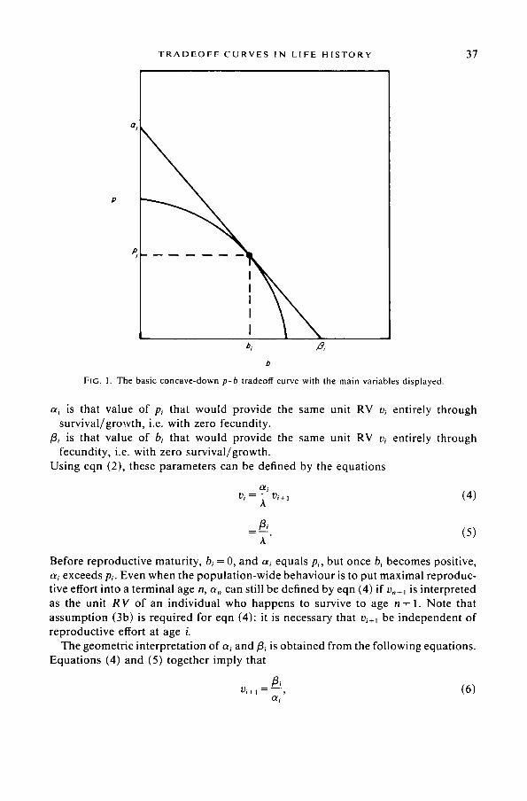
The tradeoff at each age between fecundity and survival /growth is modelled by making pi a decreasing function of b~. It is assumed that at some age m of reproductive maturity, b~ becomes positive for the first time, and stays positive from that point on, and it is assumed that at all ages i -> m, the graph ofp~ against b~ is concave-down (Fig. 1).

Now two artificial life history parameters are defined which are mathematical ly very useful, and have important geometric interpretations.


a

P

I

I

b

FIG, 1. The b a s i c c o n c a v e - d o w n p-b t r a d e o f t cu rve wi th the m a i n va r i ab l e s d i s p l a y e d .

ai is that value of Pi that would provide the same unit RV vi entirely through survival/growth, i.e. with zero fecundity.

/3i is that value of b~ that would provide the same unit RV v~ entirely through fecundity, i.e. with zero survival/growth.

Using eqn (2), these parameters can be defined by the equations

v, = ~- v,+, (4)

t3, - ( 5 )

A"

Before reproductive maturity, b~ = 0, and a~ equals p~, but once b~ becomes positive, ai exceeds p~. Even when the populat ion-wide behaviour is to put maximal reproductive effort into a terminal age n, a,, can still be defined by eqn (4) if v,+~ is interpreted as the unit R V of an individual who happens to survive to age n + 1. Note that assumption (3b) is required for eqn (4): it is necessary that v~+t be independent of reproductive effort at age i.

The geometric interpretation of ai and/3~ is obtained from the following equations. Equations (4) and (5) together imply that

13, vi+, = - - , (6)

O/i

38

and eqns (2) and (4) give us

P. T A Y L O R

bi v i + l - ( 7 )

ai - P i '

whenever b i > 0 (so that a~>pi) . It follows from (6) and (7) that a~ and fl~ are the intercepts on the p- and b-axes respectively of the line of slope -1/vi+~ through the point (b~, p~) on the tradeoff curve. In case a~ =pi , this follows from (6) alone. This interpretation will be important in our discussion of optimality conditions.

An interesting relationship is found by applying eqn (4) repeatedly over the first k age classes:

O~10~ 2. . . Olk~k+ I 1 = v~ - ;~k+~ ( 8 )

Equation (8) says that the geometric mean of the k + 1 terms in the numerator is the populat ion growth rate A. In a sense, a~ is a " 'survival-growth" measure and fl~ is a "fecundi ty" measure of how well the organism does, relative to the population growth rate A, in its ith year.

A S S U M P T I O N O N T H E A G E - D E P E N D E N T N A T U R E O F T H E p-b C U R V E S

Finally, an assumption about the change in the pi-bi curves with age is made. It is assumed that the life of the organism is divided into two stages: stage I during which pi increases with age or is constant for each fixed b, and stage II during which pi decreases with age or is constant for fixed b. Let t denote the transitional age between the stages. Thus:

Stage I (i<t) pi<--pi+l at each b ( 9 )

Stage II ( i > t) P~->Pi+~ at each b.

As an example, consider a long-lived organism whose life cycle consists of a period of physical and reproductive growth, a steady-state period of constant size and reproductive output, and a period of senescence. During the growth phase, the survival P~ increases with age at each fixed b, but at a decreasing rate, and the growth increment gi decreases at each fixed b, at an increasing rate at first, when the organism is small, and then at a decreasing rate as steady-state is approached (corresponding to a logistic type growth curve). The effect of this on the product p~ is uncertain, but it will certainly increase at the beginning and will likely start to decrease as the steady-state is approached. During the steady-state, the survival P~ and the growth increment g~ do not change with age, and hence neither will their product p~. During senescence, P~ and pi, and possibly g~ decrease with age. With this life history pattern, stage I will occupy a good part of the growth phase, and stage II will occupy the last part of this phase, and the remainder of the life.

This simple assumption of two stages may not exactly describe many organisms, but my purpose in the next section is really to develop the mathematical tools that are appropr ia te for analysing changes in life history parameters under similar assumptions.

3. The Optimality Condition: Changes in Unit RV and Fecundity with Age

T H E O P T I M A L I T Y C O N D I T I O N

The principal evolutionary problem is to find the schedule of reproductive effort which maximizes fitness. When the b - p tradeoff curves at each age are density independent, as is our assumption, then the answer to this problem is that the b~ should be chosen to maximize A given by eqn (1) (Gadgil & Bossert, 1970; Schaffer, 1974; Taylor et al. , 1974). An important general result, first proposed by Williams (1966), and demonstrated by Schaffer (1974), Taylor et al . , (1974), Schaffer (1979), Charlesworth (1980), and Caswell (1989: 176) asserts that this is the same as choosing b~ at each age to maximize v;. It is interesting to note (Schaffer, 1979) that this result requires assumption (3a) but not assumption (3b). To see this, write eqn (1) as

cc i - I

1 = ~. ljbjA - j = ~, ljbjA - j + liv,A ' - ; j = l j = l

and multiply by A ~ ~ to get

i - I

- ljbjA - = l,v,. (10) j = l

The expression on the left is a polynomial in A with leading coefficient 1, and under assumption (3a), changes in b; do not affect its coefficients. Since A is the largest root of the equation, it must increase with the right-hand side of the equation. Since l; is also unaffected by changes in b~, again by assumption (3a), the right-hand side is maximized by maximizing v~.

Differentiating eqn (2) with respect to bi:

a 13 i Opi 0 l) i + I A-~i=l+-~ivi+'+Pi Ob--'-/- (11)

Now assumption (3b) implies that v~+j is unaffected by changes in b;, and it follows that the last term of eqn (11) is zero. Hence:

O?.)i A ~-~i = 1 + ~ vi+,. (12)

If b~ denotes the value which maximizes v;, then the left-hand side of (12) must be negative when bi = 0, positive when b~ = b m~, and zero when b; is intermediate. This gives us the optimality condition

f b ~ = 0 m a x

w h e n J 0 < b i < b i , (13)

which was first formulated by Charlesworth & Leon (1976). Geometrically, this implies that the line of slope - 1 / v i + ~ through the optimum point ( b ; , p~ ) on the

40 P. TAYLOR

age-/ tradeoff curve must lie above the curve except at the opt imum point. Since we have noted that this line has p- and b-intercepts a~ and fli, we deduce that

the line with p-intercept c~ and b-intercept fl~ lies above the age i tradeoff curve except at the opt imum point. (14)

In particular, this line is tangent to the curve at the opt imum point when the opt imum fecundity is intermediate.

With this analysis, we can obtain the two conditions for the optimal value of v~ to decrease, one sufficient and one necessary, obtained by Charlesworth & Leon (1976). Their sufficient condition is

ifpmaX>h then v~>vi+l

and this follows from eqn (4) by noting that ag-> p~X. Their necessary condition, at any age i of intermediate fecundity, is

if vi > v~+t then k~bm~x> A,

where k~ is the magnitude of the slope of the p~-b~ curve where it meets the b~-axis (at bi = b~"~x). This follows from the fact that since b~ < b~ 'aX, then

max kibi > a~.

since the left-hand side is the p-intercept of the tangent line to the p-b curve at b~ = b~ 'ax, and, by (14), the right-hand side is the p-intercept of the tangent to the curve at b~, and since the curve is concave-down, the latter must be below the former.

C H A N G E S I N U N I T RV A N D F E C U N D I T Y W I T H A G E

The question of how unit RV and fecundity should change during the life cycle is now addressed, assuming optimal fecundity at each age. Two results are obtained which are proved in the Appendix. The second result requires some additional assumptions.

Theorem 1. Change in unit RV with age. For an optimal life history schedule, under the above assumptions, the vi either decrease during the entire life of the organism, or increase during the first part of the life, possibly staying constant for some period, and decrease thereafter. In either case, vi must decrease during stage II.

In particular, during any steady-state period of stage II (in which the pi-bi curves remain constant with age), unit RV will decrease.

What can we say about changes in fecundity b;? The answer is that very little can be said without further assumptions on the relation between the p~-b~ curves belonging to different ages. It 's not enough to know whether the curve at age i lies above or below the curve at age i + 1 : we have to know something about their relative shape. Of course, if there is a steady-state period in stage II, during which the p~-b~ curves remain the same, then since the curves are concave-down, changes in v~+~ from one age to the next will correspond to changes in b~ in the opposite direction, by condition (13), and hence, during any steady-state period, fecundity should increase.

An additional assumption is now made about the life history, which is strong enough to allow us to conclude that fecundity should increase during the entire reproductive life of the organism. The assumption is the strongest one possible that allows the maximum value pm,~ of the survival/growth to change with age. It is assumed that b~ ax = b m~x is independent of i, and that all the p~-b~ curves have the same "shape" , and differ only in the scaling along the p-axis. That is, it is assumed there are constants ri, such that at each fixed b,

Pi+~ = ripi. (15)

and in terms of the two stages defined in the last section [condition (9)]

stage I ( i < t ) r ,->l and ri+~<-r~ (16)

stage II ( i ->t) r~-~l.

The additional assumption that the r~ decrease or stay constant during stage I is made. That is, the factor by which the curves increase is greater earlier in life.

These new assumptions (15) and (16) on the shape of the tradeoff curves provide the following result, proved in the Appendix, about the change in fecundity and RV with age.

Theorem 2. Change in fecundity and RV. With assumptions (15) and (16), whether reproductive maturity occurs during stage I or stage II, unit fecundity bi increases and unit RV v~ decreases throughout the reproductive life of the organism.

The result we obtain here on the change in unit reproductive value is stronger than that of Theorem 1.

4. Discussion

The traditional approach to life history analysis works with the fecundity Bi and the survival P~, and, indeed, these are the usual variables that appear in the Leslie matrix. The objective of the ESS theory is to find the B - P schedule which maximizes individual fitness. However, in general, the ESS equations are not easy to analyse. A major source of difficulty comes from the effect of changes in fecundity at one age on survival or fecundity at another age. The equations are a lot simpler if changes in Bi are allowed to affect only the survival P~ at the same age. Of course, such an assumption must usually be quite unrealistic, certainly in those cases in which changes in current fecundity can affect current growth rate, and hence future size, and hence future fecundity.

In fact, this particular effect can be allowed for by treating growth rate and survival as two components of a generalized survival/growth p~ = Pg~, where g~ is the growth increment at age i. With the assumptions that fecundity is proportional to size, the ESS analysis can be done in terms of the pi and the unit fecundity b~, and the assumption that changes in current unit fecundity have no effect on the functional dependence of p~ on b~ at other ages, is not so unreasonable, in that it does allow an effect on future fecundity Bi through a change in future size. These " lower case" variables can be regarded as the entries of a generalized Leslie matrix,

42 P. TAYLOR

and the ESS analysis in terms of these is tractable when attention is restricted to tradeoffs between unit fecundity and growth/survival within each age class.

Previous studies (Schaffer, 1974; Charlesworth & Leon, 1976) have assumed that the b-p tradeoff curves remain constant, at least over the period of reproductive maturity, but the analysis here allows these curves to vary with age. It is assumed that there is an initial stage I during which the individual's performance in the game of life (surviving, growing and /o r reproducing) generally gets better, and a final stage II during which individual performance stays the same, or deteriorates. With this quite general assumption, we conclude (Theorem 1) that unit RV will either decrease during the entire life of the organism, or increase at the beginning, reach a maximum, and decrease thereafter.

The question of how unit fecundity is expected to change is more difficult, and seems to require stronger assumptions on the relation between tradeoff curves at different ages. The assumptions (15) and (16), that all the p~-bi curves are similar in shape, allow us to conclude that unit fecundity increases (and unit RV decreases) throughout the reproductive life of the organism.

The model can be made more general by letting growth increment gi represent, not only changes in size, but also changes in reproductive efficiency, such as the development of more effective reproductive mechanisms. But if the idea of a tradeoff between p and b is to continue to have any meaning, it should be the case that increases in p~ can only be obtained at the expense of b~, and so the model should only pretend to describe those improvements in reproductive efficiency which have a cost in present fecundity.

P A R E N T A L E X P E R I E N C E

Of course, there are situations in which present fecundity can actually enhance future reproductive effectiveness. One example of this is +'helping at the nest": the possibility that today's offspring will help raise those of tomorrow. Another example is parental experience: the possibility that parental effectiveness improves with practice, so that today's reproductive efforts increase tomorrow's fecundity. Such phenomena, which contribute negatively towards the correlation between present survival/growth and future fecundity, seem quite difficult to model in the framework of this paper. For example, it is not at all easy to see what effect they might have on the form of the p-b tradeoff curve. On the whole it must be difficult to predict in general how quantities such as reproductive value are expected to change early in the reproductive life, when the effects of parental experience might be significant.

C H A N G E IN R E P R O D U C T I V E V A L U E

One of the disadvantages of the p-b approach is that the RV results are actually about changes in RV per unit size. To translate these into results about changes in overall RV, we have to know how size changes with age, and this may not be so easy to describe, especially if, to make the model more general, we use si to describe a generalized notion of size, which includes increases in reproductive efficiency

TRADEOFF CURVES IN LIFE HISTORY 43

obtained at the expense of current fecundity. Of course, once the organism has attained full size, if there are not subsequent changes in (generalized) size, then RV will show the same pattern of change as unit RV, and the results of section 3 will predict changes in RV.

As an example, suppose the organism has attained full size s by the age m of reproductive maturity. What can Theorem 1 tell us? If we know that the organism has also attained full annual survival by this age, then m will belong to stage II, and we know that unit RV must decrease throughout the reproductive life. Since size is no longer increasing, we can deduce that RV itself decreases. And if we are prepared to accept the assumptions (15) and (16), that the p - b curves have a uniform shape, we can reach the same conclusion even without the condition that full annual survival be attained.

It has been empirically observed (Fisher, 1930; Hamilton, 1966) that RV tends to increase early in life, and then, close to the age of reproductive maturity, starts to decrease, and continues this decrease for the rest of the life. Because of the difficulties of modelling generalized growth, it does not seem easy to construct a realistic model which can predict this pattern over the entire life.

C H A N G E S I N P A R E N T A L I N V E S T M E N T

Another question of interest is how parental investment (PI) should change with age. Recall that PI is defined as the loss in residual RV due to present reproductive effort. First, note that eqn (2) partitions unit RV into a component bJA due to current reproduction and a residual component p~v~+j/A due to future expected fecundity. If b~ were zero, this residual component would be p~aXv~÷j/A. The difference between these is the loss in unit residual RV:

Absolute unit PI = p~X v~+ ~/A - piv~+l] A.

Note that vi+~ is the same in both occurances because it is independent of fecundity at age i [assumption (3b)]. It is actually more meaningful to work with the relative loss, which is obtained by dividing absolute unit PI by unit RV for b~ = 0. Then, the v~+~/A cancel and we are left with

m a x

Relative PI =p~ -P~ m a x Pi

and this can be interpreted on the p~-bi graph. Note that relative PI and relative unit PI are the same.

The result of Theorem 1 on the change in unit RV, does not allow us to deduce how relative PI is expected to change with age, except in the steady-state, when the p-b curves remain the same. In this case, since v~ decreases with age, and the p-b curve is concave-down, we deduce from condition (13) that the p~ decrease with age, and relative PI must increase.

Under the stronger assumptions (15) and (16), we can do better than this. Since the functions p~ = p~(b) are all proportional, relative PI is a fixed monotone-increasing function of b, the same function at all ages. Hence, when b~ increases, so does

44 p. TAYLOR

relative PI, and we deduce from Theorem 2 that relative PI is expected to increase throughout the period of reproductive maturity.

T H E M A X I M I Z A T I O N O F A

Under our assumption of density independence, a set of life history parameters which maximizes A [given by eqn (1)] will be an ESS in the sense that an alternative set of parameters which has a smaller value of A will be selectively eliminated, provided the mutant individuals are rare or deviate in behaviour by a small amount. The point of the proviso, is that the geometric growth rate A defined by eqn (1) assumes a uniform population. In a mixed populat ion, the equations for the growth rates of each of the component strategies are more complicated.

There is another proviso, and that is that the above result uses a deterministic condition for the spread of the mutant gene, whereas a stochastic analysis of its survival probabili ty would be more appropriate. According to Charlesworth & Williamson (1975) the results in the two cases are closely related.

In the density dependent case, the analogous result maximizes the carrying capacity of the environment, which is given as a function of the life history parameters, and an analogous theory to the one presented here requires a specification of the form this functional dependence might take. Further discussion of this case is found in Charlesworth & Leon (1976) and Hastings (1978).

R E P R O D U C T I V E E F F O R T

The model used here has been referred to as the reproductive effort (RE) model (Charlesworth & Leon, 1976) but in fact reproductive effort is rarely very well defined, and, in this paper, it simply serves to provide an interpretation for the underlying parameter e~ for the tradeoff between fecundity and survival/growth. Mathematically, we regard survival /growth as a function of unit fecundity, and bypass RE altogether. What ecologists mean by RE is often closely associated with time and energy budgets and risk taking, and the relation between that and fecundity or PI is often not clear, and is certainly expected to change with age. However, these same ecologists are interested in the question of when RE is expected to increase or decrease with age. To get theorems of this nature requires an assumption on how RE at each age relates to the unit fecundity bi, and I am not certain at this point what kind of patterns are appropriate. There seems to be little work done on this question.

ASSUMPTIONS ON THE SHAPE OF THE p-b CURVES

The assumptions on the form of the tradeoff curves may not be unreasonable, but it is difficult to get good evidence on this matter. It is even difficult to get evidence that the tradeoff curves are concave-down (Charlesworth, 1980: 5.3), although the theory predicts that if this is not the case, the optimal strategy must have either zero fecundity, or zero survival. In fact there is even a scarcity of evidence

T R A D E O F F C U R V E S IN LIFE H I S T O R Y 45

fo r t he r e p r o d u c t i v e cos t m o d e l i tself . C h a r l e s w o r t h (1980: 5.3) a n d Bell &

K o u f o p a n o u (1986) s u m m a r i z e s o m e o f the e v i d e n c e tha t is ava i l ab l e . O n e b ig

p r o b l e m , o f cou r se , is t ha t any a t t e m p t to l o o k for a n e g a t i v e c o r r e l a t i o n b e t w e e n

f e c u n d i t y a n d su rv iva l w i t h i n a p o p u l a t i o n , will be s w a m p e d by the pos i t i ve co r re l a -

t i on b e t w e e n t he se v a r i a b l e s g e n e r a t e d by the e x i s t e n c e o f i n d i v i d u a l s o f v a r i a b l e

na tu r a l p r o w e s s o r v igou r . O n e mus t resor t e i t h e r to an e x p e r i m e n t a l a p p r o a c h , o r

to c o m p a r i s o n s b e t w e e n spec i e s (Bel l & K o u f o p a n o u , 1986).

I am grateful to Bob Montgomer ie for his col laborat ion in our attempts to understand the biological significance of the mathematical results. This work was supported by a grant from the Natural Sciences and Engineering Research Council of Canada.

R E F E R E N C E S

BELL, G. (1980). The cost of reproduction and their consequences. Am. Nat. 116, 45-76. BELL, G. & KOUFOPANOU, V. (1986). The cost of reproduction. Oxford Surveys Evol. Biol. 3, 83-131. CASWELL, H. (1989). Matrix" Population Models. Sunderland, MA: Sinauer. CHARLESWORTH, B. (1980). Evolution in Age-structured Populations. Cambridge: Cambridge Studies in

Mathematical Biology. CHARLESWORTH, B. & LEON, J. A. (1976). The relation of reproductive effort to age. Am. Nat. II0,

449-459. CHARLESWORTH, B. & WILLIAMSON, J. A. (1975). The probability of survival of a mutant gene in an

age-structured population and implications for the evolution of life histories. Genet. Res. 26, 1-10. FISHER, R. A. (1930). The Genetical Theo o, of Natural Selection. Oxford: Clarendon Press (Reprinted

and revised, 1958). GADGIL, M. & BOSSERT, W. H. (1970). Life historical consequences of natural selection. Am. Nat. 104,

1-24. HAMILTON, W. U. (1966). The moulding of senescence by natural selection. J. theor. Biol. 12, 12-45. HASTINGS, A. (1978). Evolutionarily stable strategies and the evolution of life history strategies: I.

density dependent models. J. theor. Biol. 75, 527-536. SCHAFEER, W. M. (1974). Selection for optimal life histories: the effects of age structure. Ecology 55,

291-303. S(.'HAFFER, W. M. (1979). Equivalence of maximizing reproductive value and fitness in the case of

reproductive strategies. Proc. HatH. Acad. Sci. U.S.A. 76, 3567-3569. TAYLOR, H. M., GOURLEY, R. S. & LAWRENCE, C. E. (1974). Natural selection of life-history attributes:

an analytical approach. Theor. pop. Biol. 5, 104-122. WILLIAMS, G. C. (1966). Natural selection, the costs of reproduction, and a refinement of Lack's

principle. Am. Nat. 100, 687-690.

A P P E N D I X

P r o o f o f T h e o r e m 1

T h e T h e o r e m is p r o v e d by w o r k i n g b a c k w a r d s s t a r t ing at the t e r m i n a l age n at

w h i c h b, = b,m, ~x. It is s h o w n first tha t

a, ,_l > A. (A.1)

It is t h e n s h o w n tha t d u r i n g s tage II ( t A ==~ cei_l > A , (A.2)

a n d d u r i n g s tage I (1 Ot'i_l ( A. (A.4)

46 p. TAYLOR

These three conditions imply that t~, > )t during stage II, and that the entire life can be divided into three chronological phases, the first when ai < )t, the second when t~ = )t, and the third, when a~ > A, except that one or both of the first two phases may be absent. Theorem 1 then follows from eqn (4).

I begin with (A.1). Since b,_~ is intermediate, and the tradeoff curve is concave- down,

fl,,_,> bm~>__b max,

where the second inequality comes from the defining assumption (9) of stage II. Thus, from eqn (6),

ft._, b ~ "~X V n ~- ~ - - .

O l n - I Oln 1

Since v, = b~X/A [eqn (2)], we conclude that c~,,_~ > A. Condit ions (A.2-A.4) are proved by establishing a pair of stronger conditions:

stage II ( t ai_l ~ a , _ t > A (A.5)

stage I ( l A but a~_~ <-A. It follows that a, > ai_t , and (A.5) implies that a~_~ > A which is a contradiction. The arguments for (A.3) and (A.4) are similar.

The demonstrat ions of (A.5) and (A.6) are completely parallel, and (A.5) is demonstrated. A useful piece of terminology is to call the line with b- and p-intercepts fl~ and a~ the i line, and the p-b tradeoff curve at age i the i curve.

Suppose a~ > a~_~. It follows from this that /3~ </3i_t. Otherwise, /3~->/3~_~, and it follows that the i - 1 line lies below the i line at b~, the optimal fecundity at age i. (Here, b , < b ~ a~ is needed, which holds since i < n.) But the i - 1 line lies above the i - 1 curve, and the i line touches the i curve at b~ [condition (14)] and it follows that the i - 1 curve lies below the i curve at bi, contradicting (9) for stage II. It follows that/3i </3~_~. To complete the argument, note that, by eqns (5) and (6),

/3, /3,_, - - - ( A . 7 )

A °ti I '

and it follows that a , _ t > h.

P r o o f o f T h e o r e m 2

We begin with a technical result which lists a number of equivalents to the condition that fecundity increase from age i - 1 to age i.

I f 0 < bi bi-i

(ii) cei> ri_toq_t

(iii) vi>ri tv/+~

(iv) a i > ri-lh.

(A.S)

To see that (i) is equivalent to (ii) and (iii), refer to Fig. A1. Since bi is an interior op t imum, the tangent to the /-curve at bi has slope -1/vi+, and p-intercept ai. I f we mult iply all heights by 1/r~_~ we get the i - 1 curve and a line which is tangent to it at b~ with slope -1/r i - ,v i+, , and p- intercept a~/r~_~. Since the i - 1 curve is concave-down, b~_~ will be less than bi precisely when the tangent to the i - 1 curve at b~_, has a lower p- intercept and is less steep than the tangent (to the i - 1 curve) at b~. And that 's condi t ions (ii) and (iii).

To show that (iii) and (iv) are equivalent, (iii) can be written

ri-t vi+t < vi = bi+p/vi+1, A A

using eqn (2), and this can be written as

bi l')i+l <" r i - lA --Pi

Equation (7) tells us that this is equivalent to (iv). Now we turn to the proof of T h e o r e m 2. Looking first at stage II, the result of

T h e o r e m 1 is that unit RV decreases during this stage: v~ > vi+~ f o r i >- t. Since r~_~ -< 1 f o r i > t, it follows that v~> r~_lV~+, f o r i > t. But this is condit ion (A.8ii i) above, and it follows that b~ > b~_~ for t b,_~ since b, is maximal, but b,_~ is not.

a i

r i _ , S l o p e - I / r , . _ r v i ÷ ,

Slope - I /v i+ ,

FIG. AI. An illustration of the equivalences of (A.8). The picture has been drawn with the ( i - 1 )-curve above the /-curve, but the argument works when they are reversed.

48 P. TAYLOR

N o w look at stage I, assuming reproduct ive life commences dur ing this stage, that is, m < t. Since b,,_l = 0, we certainly have that b,, > b,~_j and hence, by (A.8iv), a , , > rm_lA. Since r,,_l -> 1, we deduce that a, , > A. It follows from (the contraposi t ive of) (A.6), with m = i - l , that am+~>-am and hence that a m + l > A. Cont inuing inductively, using (A.6), we find that ai > A for m <- i--< t, and that ai is constant or increasing. Since ri is constant or decreasing dur ing this same period, the inequali ty cti>r~_iA must cont inue to hold for m<-i<-t . It follows from (A.8) that the b~ increase dur ing this period. Along the way we have seen that c~ > A during the reproduct ive port ion o f stage I, and hence, by eqn (4), the v~ decrease.

optimal life histories with age dependent tradeoff curves i

Documents