optimal lot size in a manufacturing system with imperfect

Scientia Iranica E (2019) 26(4), 2561{2578

Sharif University of TechnologyScientia Iranica

Transactions E: Industrial Engineeringhttp://scientiairanica.sharif.edu

Optimal lot size in a manufacturing system withimperfect raw materials and defective �nished products

H. Mokhtari�

Department of Industrial Engineering, Faculty of Engineering, University of Kashan, Kashan, P.O. Box 8731753153, Iran.

Received 14 December 2017; received in revised form 10 April 2018; accepted 5 May 2018

KEYWORDSManufacturingsystems;Manufacturingplanning;Imperfect rawmaterial;Defective �nishedproduct;Reworking process.

Abstract. In real-world manufacturing systems, it is inevitable to encounter imperfectraw materials and generate defective �nished products. In order to cope with these practicalproblems, this paper studies a manufacturer that orders raw materials from an externalsource (supplier) and, then, produces a �nished product. The raw materials containimperfect quality items; in addition, the production system is defective. The imperfectraw materials are sold after the screening process, while the defective �nished products gounder a further rework process. It is also assumed that the defective rate of a machine is arandom variable, resulting in three possible cases regarding the occurrence of backorderingshortage. The aim is to determine economic order/production lot sizes for each case in sucha way that the total cost of the system is minimized. The optimal closed-form solution isderived for each case separately. Moreover, the applicability of the proposed manufacturingmodel is illustrated via a numerical example.

© 2019 Sharif University of Technology. All rights reserved.

1. Introduction

One of the basic and useful production-inventory plan-ning models is the Economic Order Quantity (EOQ).The aim of EOQ is to �nd economic lot size of materialsto order from external sources so as to minimizethe total cost of a system composed of holding andordering costs. The classic EOQ was customizedfor manufacturing settings through economic pro-duction/manufacturing quantity (EPQ/EMQ) models.The traditional models of EOQ/EPQ are based onsome simple assumptions such as:

(i) Demand rate for an item is pre-known andconstant;

*. Tel.: +98 031 55912476E-mail address: mokhtari [email protected]

doi: 10.24200/sci.2018.50013.1464

(ii) All order quantities are received instantaneous-lyfor EOQ and, gradually, for EPQ;

(iii) Items are entirely consumed when the next orderis received;

(iv) Shortage is not permitted and no safety stock isallowed;

((v) There is no quantity discount;

(vi) Ordering/setup cost is �xed per order/produc-tion;

(vii) All parameters are deterministic;

(viii) All received/produced items are of perfect qual-ity.

Since holding and ordering costs behave inversely in ba-sic EOQ/EPQ models, the total cost function is convexand, then, an intermediate amount of lot size is opti-mal. Based on the above assumptions, closed-form lotsizing can be simply calculated for the basic EOQ/EPQ

2562 H. Mokhtari/Scientia Iranica, Transactions E: Industrial Engineering 26 (2019) 2561{2578

models. The above assumptions are far from realconditions to justify the use of basic EOQ/EPQ modelsin practice. Therefore, a large body of literature hasbeen allocated to relaxing these assumptions.

One of the assumptions in the manufacturingplanning models, such as EPQ which is unrealistic, isthat all items (raw materials received from externalsources and �nished products by own manufacturer)are of perfect quality and conform to all requiredcharacteristics perfectly. However, in reality, thisassumption is not necessarily true and is a crucialweakness of traditional manufacturing models. Forthis reason, the problem of imperfect quality itemshas received the attention of researchers during recentyears. Porteus [1] analyzed production lines in theout-of-control state when products are of imperfectquality and the rate of defective items is dependenton lot size. Moreover, Rosenblatt and Lee [2] studiedthe EPQ model with an imperfect process. Salamehand Jaber [3] did a great improvement in imperfectquality context by proposing an EOQ model consid-ering a 100% inspection process upon receiving theproducts to identify defective products. The researchof Salameh and Jaber [3] was modi�ed by C�ardenas-Barr�on [4] and Maddah and Jaber [5]. Rezaei [6]developed an inventory model with imperfect qualityof items and fully backordered shortage. In addition,Yu et al. [7] extended the inventory model, which isimperfect with mixed partial backordering shortageand lost sales. Then, Wee et al. [8] studied theEPQ model with an imperfect quality alongside therate of deterioration and partial backordering short-age. In addition, Papachristos and Konstantaras [9]proposed an inventory model with a constraint toavoid shortages. Moreover, Wee et al. [10] proposedan inventory model with fully backordering shortage.Khan et al. [11] presented a review of imperfect qualityinventory models. At the same time, Wahab et al. [12]derived a coordinated level supply with shortages andenvironmental e�ects considering imperfect quality ofitems. Afterward, Konstantaras et al. [13] studied theimpact of learning e�ect on the number of imperfectproducts and lot size. Liu and Zheng [14] suggesteda fuzzy model with inspection errors in imperfectproducts. Moreover, Hsu and Hsu [15] proposed ageneral model for imperfect products with inspectionerrors, backordering shortage, and sales returns. Inaddition, Rad et al. [16] derived a price-dependentdemand model for an integrated supply chain withan imperfect process and allowed shortage. Skouriet al. [17] developed an EOQ inventory model withimperfect products in the received lot and rejection ofimperfect items to a supplier. In another work, Paulet al. [18] presented a joint replenishment problem todetermine the lot size for products with defective items.Hlioui et al. [19] investigated a supply chain model with

defective items with 100% screening. Shari� et al. [20]studied the e�ect of inspection errors on inventorymodels with imperfect items and partial backorderingshortage. Alamri et al. [21] evaluated the impactof learning on the inventory model with imperfectitems. Chang et al. [22] developed an extension tothe inventory model with imperfect items consideringpermissible delays in payments and inspection errors.Rezaei [23] proposed using sample inspection insteadof full inspection in inventory models with imper-fect items. Yu and Hsu [24] proposed an unequalsized shipment for a production-inventory problemwith 100% inspection and item return. Sarkar andSaren [25] investigated warranty cost through the EPQmodel considering defective items along with inspectionerror. Ongkunaruk et al. [26] proposed consider-ing some constraints, such as shipment, budget, andtransportation capacity constraints, in an inventorymodel with defective items. Taleizadeh et al. [27]proposed an imperfect EPQ manufacturing model withbackordering allowed and trade credits. Cheikhrouhouet al. [28] proposed joint optimization of sample sizeand order size considering lot inspection policy andthe withdrawing of defective batches. Taleizadeh andZamani Dehkordi [29] considered an economic orderquantity model with partial backordering and samplinginspection. Mokhtari and Rezvan [30] discussed aproduction-inventory system under VMI condition andpartial backordering. Jaber et al. [31] extended thework of Salameh and Jaber [3] by proposing economicorder quantity models considering imperfect items andbuy and repair options when encountering a distantsupplier. In addition to the above literature, a newdirection of researches appears that considers random-ness in the production system of the EPQ model.Chiu et al. [32] extended the economic productionquantity model with nonconforming items for a casewith random machine breakdown. Bouslah et al. [33]proposed joint lot sizing and production policy in anunreliable manufacturing system with random failureand repair. Mokhtari et al. [34] proposed the economicproduction quantity model for perishable productswith stock-dependent demand and shortage backo-rdered. Moreover, Tayyab and Sarkar [35] proposed amulti-stage production system with a random defectiverate. Mokhtari [36] suggested a joint decision problemconsisting of internal production replenishment and lot-sizing optimization with supplier selection, consideringdefective manufacturing and rework option.

This paper proposes a production-inventorymodel where a manufacturer orders raw materials froman external source (supplier) and produces a �nishedproduct via a �nite production rate. The raw materialscontain imperfect quality items; hence, a 100% screen-ing process is implemented on lot-size receipt. On theother hand, the production system is also defective,

H. Mokhtari/Scientia Iranica, Transactions E: Industrial Engineering 26 (2019) 2561{2578 2563

and a fraction of �nished products is imperfect. Theimperfect raw materials are sold after the screeningprocess, while the defective �nished products go undera further rework process on the same machine. Anumber of defective products are reworkable and havethe potential to become perfect after the reworkingprocess, while others are scrapped items and sold ata lower price. It is also assumed that the defectiverate of a machine is a random variable, resultingin three possible cases regarding the occurrence ofbackordering shortage. Here, two scenarios for eachcase are designed, resulting in six total states. The aimis to determine economic order/production lot sizes foreach case in order to minimize the total cost of thesystem.

The rest of this paper is structured as follows.Section 2 presents the overall description of the prob-lem and introduces the proposed manufacturing modelsvia three possible cases. Then, Section 3 discussesnumerical experiments. Finally, Section 4 presentsconclusions.

2. Manufacturing system modeling

2.1. Overall description and notationsA new manufacturing model is proposed based onwhich a manufacturer produces a product to satisfyan external demand, D. The demand is assumed tobe constant over a time horizon. The manufacturerproduces the product via a �nite production rate, P1,under EPQ setting. In addition, the shortage is notallowed and purchase cost is �xed. In contrast tothe standard models, it is assumed that the produc-tion system is defective and produces a percentageof imperfect items, �. The imperfect items are alsounder a rework process to become perfect and return tothe consumption cycle. In general, an inventory cycleis composed of production, reworking, and depletionperiods. After a production period, a percentage ofdefective items, �, which are reworkable, go under therework process with rework rate, P2. In real-worldsituations, many environmental features a�ect the pro-duction system and cause a uctuation in the qualityof produced items. Hence, as a realistic assumption,it is considered that the percentage of defective items,�, is a random variable. At the end of the reworkperiod, the stored inventory is consumed until reachingzero during the depletion period. The production iscarried out via production rate, P1, within productionperiod, tp. Once the production ends, there existimperfect items, �Q. Among them, the reworkableitems, ��Q, go under the reworking process, andthe scrapped items, (1 � �)�Q, are disposed fromthe system. During the rework period tR, all thereworkable items, ��Q, become perfect with the rateof P2 and return to the system. At the end of the

rework period, the stored inventory is consumed duringdepletion period, tD, until reaching zero. The nextcycles repeat this process continuously. The aim is todetermine optimal/economic production quantity, Q,such that the total pro�t is maximized. The total pro�tper cycle, TP , is obtained as the total revenue per cycleTR minus the total cost per cycle, TC.

Herein, three possible cases (I, II, III) regardingthe occurrence of shortage in the proposed system areanalyzed. In Case I, shortage does not occur; therefore,the initial condition is considered as Imax � �Q � 0.Since Imax = Q(1�D=P1), this condition is simpli�edto:

0 � � � 1� DP1: (1)

In Case II, shortage occurs, yet is backordered fully.In this case, a shortage is encountered due to (1 �D=P1) � � < 0; however, it is backordered becausethe number of reworked items minus demand duringthe rework period is greater than that of shortage, i.e.,(1�D=P1)� � +��(1�D=P2) > 0. These conditionsare summarized as follows:

1� DP1

< � <1�D=P1

1� �(1�D=P2): (2)

Finally, in Case III, not only shortage occurs, but alsothe number of reworked items is not su�cient to coverall shortages occurred. In this case, there will be anamount of unsatis�ed demand. To prevent lost sale, aspecial order is used at the end of the rework period(will be discussed later). The condition for this case isas follows:

1�D=P1

1� �(1�D=P2)� � � 1: (3)

A famous condition in an EPQ model is that produc-tion rate P should be greater than demand rate, D,in the classic EPQ model (P > D). This conditionensures model feasibility and prevents severe shortagein all planning horizons. Conditions I-III play sucha role in our model and should be checked beforestarting to solve the problem. Of course, the expectedvalue of defective items should be considered in theseconstraints, since it is a random variable.

Before formulating the problem, the notationsused throughout the paper are summarized as follows:

D The demand rate of �nished products;P1 The production rate of �nished

products;P2 The rework rate of �nished products;A1 The �xed order cost of raw materials;


A2 The �xed setup cost of �nishedproducts;

h1 The holding cost of raw materials peritem per unit time;

h2 The holding cost of �nished productsper item per unit time;

C1 The purchase cost of raw materials peritem;

C2 The production cost of �nishedproducts per item;

d1 The screening cost of raw materials peritem;

d2 The screening cost of �nished productsper item;

r The rework cost of �nished productsper item;

p The selling price of imperfect rawmaterials per item;

v The selling price of perfect �nishedproducts per item;

s The selling price of scrapped �nishedproducts per item;

x The screening rate of raw materials;� The defective rate of �nished products;� The reworkable rate of defective

�nished products;q The imperfect rate of raw materials;tS The duration of screening period of

raw materials;tP The duration of the production period

of �nished products;tR The duration of the rework period of

�nished products;tD The duration of the depletion period of

�nished products;E[:] The expected value of random variable;Y The order quantity of raw materials;Q The production quantity of �nished

products;b The backorder quantity of �nished

products.

2.2. Case I: When shortage does not occurFigure 1 shows one cycle of the proposed manufac-turing system in Case I. To encounter the complexityof modeling a procedure gradually, two scenarios ofthis case in the sequel are considered. In the �rstscenario, the �nished product cycle is only consid-ered, while the raw material cycle is not considered.However, in the second scenario, both raw materialsand �nished product cycles are considered, simultane-ously.

Figure 1. The inventory level for manufacturing systemin Case I.

In the �rst scenario, production quantity, Q,is assumed to be a decision variable, independently.Hence, the total revenue per cycle, TRI , involves salesof perfect and scrapped items given as TRI = vfQ ��Q + ��Qg + sf(1 � �)�Qg, where v and s representthe unit selling prices of perfect and scrapped �nishedproducts, respectively. Note that the unit selling priceof perfect products is greater than that of scrappeditems (v > s). The total cost in this case involvesproduction, setup, holding, screening, and reworkingcosts. The production cost per cycle, PCI , is calculatedas PCI = C2Q. In addition, setup cost SCI isincurred per production cycle by SCI = A2. Moreover,in order to formulate the holding cost, the area atthe inventory level in three periods, i.e., productionperiod, S1, rework period, S2, and depletion period,S3, is �rst calculated. The �rst area is calculatedas S1 = Imax:tp=2. Since Imax = Q(1 � D=P1) andtp = Q=P1, S1 is re-written as S1 = Q2

2P1(1 � D=P1).

To calculate S2, the inventory level at the start ofrework period, I2, and that at the end of rework period,I3, as in I2 = Q(1 � D=P1) � �Q and I3 = Q(1 �D=P1) � �Q + (P2 �D)tR should be �rst formulated.During rework period tR, reworkable items, ��Q, arein the reworking process. Hence, tR in terms of modelparameters can be calculated as in tR = ��Q=P2.Therefore, inventory level I3 can be simpli�ed as inI3 = Q(1�D=P1)� �Q+��Q(1�D=P2). Therefore,the area at the inventory level in the rework period iscalculated as in S2 = tR(I2 + I3)=2, which can be re-written as S2 = ��Q

2P2f2Q(1�D=P1)� 2�Q+��Q(1�

D=P2)g. Moreover, the area at the inventory level inthe depletion period is formulated as S3 = I3tD=2where the depletion period is tD = I3=D; hence, wehave S3 = I2

3=2D which is re-written as follows:

S3 =1

2D

�Q(1�D=P1)��Q+��Q(1�D=P2)

�2

:

By utilizing S1, S2, and S3, the holding cost isformulated by h2fS1 + S2 + S3g as follows:


HCI =h2Q2�G2

2D+

12P1

�1� D

P1

�+��2P2

��1� D

P1

�� +G

��; (4)

where h2 is the holding cost per item per unit time andG = (1�D=P1)��+��(1�D=P2). The screening costper cycle WCI is computed as WCI = d2Q in which d2represents the screening cost of �nished products peritem. Moreover, the reworking cost per cycle, RCI , isobtained through RCI = r��Q, where r denotes therework cost per item.

Therefore, the total cost per cycle is obtainedthrough PCI + SCI +HCI +WCI +RCI as follows:

TCI =C2Q+A2 + h2Q2�G2

2D+

12P1

�1� D

P1

�+��2P2

��1� D

P1

��+G

��+d2Q+r��Q:(5)

Here, the total pro�t per cycle in the �rst scenario ofCase I, TPI , can be calculated by TRI�TCI as follows:

TPI =vfQ� �Q+ ��Qg+ sf(1� �)�Qg � C2Q

�A2 � h2Q2�G2

2D+

12P1

�1� D

P1

�+��2P2

��1� D

P1

��+G

��d2Q�r��Q: (6)

Since � is random variable, it should be replaced withexpected value E[�] in TPI to calculate expected totalpro�t, E[TPI ], as follows:

E[TPI ] = vfQ�E[�]Q+�E[�]Qg+sf(1��)E[�]Qg

� C2Q�A2 � h2Q2�

E[G]2

2D+

12P1

�1� D

P1

�+�E[�]2P2

��1� D

P1

�� E[�] + E[G]

�� d2Q

� r�E[�]Q; (7)

where E[G] = (1 � D=P1) � E[�] + �E[�](1 � D=P2).Moreover, cycle time TI is also a random variable,

which can be obtained by TI = tP + tR + tD as TI =QD (�(�� 1) + 1), whose expected value is calculated asfollows:

E[TI ] =QD

(E[�](�� 1) + 1):

Hence, the expected total pro�t per unit time is givenas follows:

E[TPUI ] =E[TPI ]E[TI ]

: (8)

By simplifying the expressions in Eq. (8), we obtain:

E[TPUI ] =D

E[�](�� 1) + 1fvf1� E[�] + �E[�]g

+ sf(1� �)E[�]g � C2 � A2

Q

� h2Q�

E[G]2

2D+

12P1

�1� D

P1

�+�E[�]2P2

��1� D

P1

�� E[�] + E[G]

�� d2 � r�E[�]g: (9)

The above expected total pro�t per unit time E[TPUI ]is concave, because:

@2E[TPUI ]@Q2 =

�2A2DQ3fE[�](�� 1) + 1g � 0: (10)

Therefore, the �rst derivative of E[TPUI ] can be set tozero so as to reach the economic lot size by Eq. (11)as shown in Box I. Here, the second scenario with bothraw material and �nished product cycles is considered.In this scenario, order quantity of raw material, Y ,is the decision variable, and production quantity of�nished product, Q, is the dependent variable. Sincea fraction of raw material, q, is imperfect, then therelationship between order and production quantities isgiven as Q = (1�q)Y . After receiving many raw mate-rials from an external source, a 100% screening processstarts; simultaneously, the perfect raw materials goto production system under rate of P1. This processcontinues until all of raw materials are inspected. Sincethe screening rate is constant, x, the duration of the

Q�I =

24 2A2D

h2

nE[G]2 + D

P1

�1� D

P1

�+ �DE[�]

P2

n�1� D

P1

�� E[�] + E[G]oo35 1

2

: (11)

Box I


screening period is calculated, tS = Y=x. Moreover, thequantity of produced items during the screening periodis tSP1. In addition, the inventory level after disposal(selling) of imperfect raw materials is obtained throughI1 = Y �tSP1�qY , which is simpli�ed, by substitutingtS , to I1 = (1 � q � P1=x)Y . The production period,tp, is the time interval at which production quantity,Q = (1 � q)Y , is processed. Therefore, it is computedas tp = Q=P1 or equivalently tp = (1 � q)Y=P1. Inthis scenario, the total revenue per cycle, TRI , involvessales of perfect and scrapped �nished products andimperfect raw materials given as:

TRI =vf(1� q)Y � �(1� q)Y + ��(1� q)Y g+ sf(1� �)�(1� q)Y g+ pqY:

The total cost, in this scenario, is associated with twocycles, i.e., �nished product cycle and raw materialcycles. The total cost of �nished product, TCfp,similar to that of the �rst scenario, involves production,setup, holding, screening, and reworking costs. Hence,it can be simply obtained by substituting Q = (1�q)Yinto the total cost of the �rst scenario as follows:

TCfp =C2(1� q)Y +A2

+ h2(1� q)2Y 2�G2

2D+

12P1

�1� D

P1

�+��2P2

��1� D

P1

�� +G

��+ d2(1� q)Y + r��(1� q)Y: (12)

The total cost of raw material cycle, TCrm, involvespurchasing, ordering, holding, and screening costs. Thepurchasing cost of raw material per cycle is calculatedas C1Y . In addition, the ordering cost is incurredper cycle as A1. Moreover, in order to formulate theholding cost, the area at the inventory level in twoperiods, i.e., screening period S1 and after screeningperiod (till end of production period) S2, is �rstcalculated. The �rst area is calculated as in S1 =fY +(qY +I1)gtS=2. By substituting I1 and tS into S1,it is simpli�ed to Y 2(2 � P1=x)=(2x). In addition, thesecond area, S2, is formulated as S2 = I2

1=(2P1), whichis simpli�ed to S2 = Y 2(1� q � P1=x)2=(2P1). Hence,the total area as in S1 +S2 = Y 2f(1�q)2=(2P1)+q=xgcan be calculated. Therefore, the holding cost of rawmaterial is formulated as follows:

HCrm = h1Y 2�

(1� q)2

2P1+qx

�: (13)

Now, the screening cost of raw material is calculatedby d1Y . Thus, the total cost of raw material cycle isobtained as follows:

TCrm=C1Y +A1+h1Y 2�

(1� q)2

2P1+qx

�+ d1Y:

(14)

Therefore, the total cost per cycle in the secondscenario is obtained by TCfp + TCrm as follows:

TCI =fC1 + C2(1� q)gY +A1 +A2

+ h1Y 2�

(1� q)2

2P1+qx

�+ h2(1� q)2Y 2

�G2

2D+

12P1

�1� D

P1

�+��2P2

��1� D

P1

�� +G

��+ d1Y + d2(1� q)Y + r��(1� q)Y: (15)

Then, the total pro�t per cycle in the second scenarioof Case I can be calculated by TRI � TCI as follows:TPI =vf(1� q)Y � �(1� q)Y + ��(1� q)Y g

+ sf(1� �)�(1� q)Y g+ pqY

� fC1 + C2(1� q)gY �A1 �A2

� h1Y 2�

(1� q)2

2P1+qx

�� h2(1� q)2Y 2

�G2

2D+

12P1

�1� D

P1

�+��2P2

��1� D

P1

�� +G

�� d1Y � d2(1� q)Y � r��(1� q)Y: (16)

Since � is a random variable, it should be replaced withexpected value E[�] in TPI to calculate expected totalpro�t, E[TPI ], as follows:TPI =vf(1� q)Y � E[�](1� q)Y + �E[�](1� q)Y g

+ sf(1� �)E[�](1� q)Y g+ pqY

� fC1 + C2(1� q)gY �A1 �A2

� h1Y 2�

(1� q)2

2P1+qx

�� h2(1� q)2Y 2

�E[G]2

2D+

12P1

�1� D

P1

�+�E[�]2P2

��1� D

P1

�� E[�] + E[G]

�� d1Y �d2(1� q)Y �r�E[�](1� q)Y: (17)


Moreover, cycle time TI , similar to that of the �rstscenario, is calculated as in TI = Q

D (E[�](� � 1) + 1)where Q = (1 � q)Y . Hence, the expected total pro�tper unit time is given as follows:

E[TPUI ] =E[TPI ]E[TI ]

: (18)


E[TPUI ] =D

E[�](�� 1) + 1

(vf1� E[�] + �E[�]g

+sf(1��)E[�]g+ pq1�q�

C1

1�q�C2� A1+A2

(1�q)Y

� h1

1� q Y�

(1� q)2

2P1+qx

�h2(1� q)Y

�E[G]2

2D

+1

2P1

�1� D

P1

�+�E[�]2P2

��1� D

P1

�� E[�]

+E[G]gg � d1

1� q � d2 � r�E[�]

): (19)

The above expected total pro�t per unit time,E[TPUI ], is concave, because:

@2E[TPUI ]@Y 2 =

�2(A1 +A2)D(1� q)Y 3 fE[�](�� 1) + 1g � 0:(20)

Thus, the �rst derivative of E[TPUI ] can be set to zeroso as to reach the economic lot size by Eq. (21) as shownin Box II.

2.3. Case II: When shortage occurs and isfully backordered

In addition, Figure 2 depicts the inventory level inCase II. Similar to the previous case, two scenariosof this case in the sequel are considered. In the �rstscenario, the �nished product cycle is only consideredand the raw material cycle is not considered, while,in the second scenario, both raw material and �nishedproduct cycles are considered, simultaneously.

Herein, the �rst scenario of Case II is addressed.Note that tR1 and tR2 represent the rework periodswhen inventory level is less than and greater than zero,respectively (tR = tR1 + tR2). The total revenue per

Figure 2. The inventory level for manufacturing systemin Case II.

cycle in this case TRII is similar to that of Case I, i.e.,the sum of sales of perfect and reworked items and salesof scrapped items, given by TRII = vfQ��Q+��Qg+sf(1 � �)�Qg. The total cost in this case involvesproduction, setup, holding, shortage, screening, andreworking costs. The production and setup costs percycle are calculated as in PCII = C2Q and SCII = A2.The area at the inventory level is classi�ed into threeperiods, i.e., production period, S1, rework periodwhen inventory level is positive, S2, and depletionperiod, S3. The �rst area calculated as S1 is similarto that of Case I which is given as S1 = Q2

2P1(1�D=P1).

To calculate S2, the inventory level at the end of therework period (start of the depletion period) via I2 =Q(1�D=P1)��Q+(P2�D)tR should be �rst obtained.By substituting tR = ��Q=P2 into I2, it is simpli�ed toI2 = Q(1�D=P1)� �Q+��Q(1�D=P2). Therefore,the area at the inventory level in the rework period iscalculated as in S2 = I2:tR2=2. Since tR1 is the timeat which shortage quantity, b = �Q�Q(1�D=P1), isfully covered by reworked items, it can be calculatedas in tR1 = b=(P2 � D), which can be re-written astR1 = f�Q �Q(1 �D=P1)g=(P2 �D). Therefore, tR2can be attained by tR � tR1, which is summarized astR2 = ��Q=P2�f�Q�Q(1�D=P1)g=(P2�D). Hence,S2 can be expressed as follows:

S2 =Q2

2(P2 �D)

��1� D

P1

�� + ��

�1� D

P2

��P2� � +

�1� D

P1

��: (22)

Y �I =

24 2(A1 +A2)D

h1Dn

(1�q)2

P1+ 2q

x

o+ h2(1� q)2

nE[G]2 + D

P1

�1� D

P1

�+ �DE[�]

P2

n�1� D

P1

�� E[�] + E[G]oo35 1

2

: (21)

Box II


Moreover, the area at the inventory level of the de-pletion period is formulated as S3 = I2:tD=2 wheredepletion period tD is I2=D; hence, we have S3 =I22=(2D). By substituting I2 into S3, it can be re-

written as:

S3 =1

2DfQ(1�D=P1)��Q+��Q(1�D=P2)g2:

By using S1, S2, and S3, the holding cost is formulatedas follows:

HCII =h2Q2�

12P1

�1� D

P1

�+

G2(P2 �D)�

��P2� � +

�1� D

P1

��+G2

2D

�: (23)

In addition, the shortage cost is calculated as inKCII =�:b:tR1=2 where � denotes the shortage cost per unittime per item. It can be re-expressed as follows:

KCII = �Q2

P2 �D��

�1� D

P1

��2

: (24)

The screening and reworking costs per cycle are com-puted as in WCII = d2Q and RCI = r��Q, similar tothose of Case I.

Therefore, the total cost per cycle in Case II isattained by PCII +SCII +HCII +KCII +WCII +RCIIas follows:

TCII =C2Q+A2 + h2Q2�

12P1

�1� D

P1

�+

G2(P2�D)

��P2�� +

�1� D

P1

��+G2

2D

�+ �

Q2

P2�D��

1� DP1

��2

+d2Q+r��Q:(25)

Here, the total pro�t per cycle in Case II is calculatedas follows:

TPII =vfQ� �Q+ ��Qg+ sf(1� �)�Qg

� C2Q�A2 � h2Q2�

12P1

�1� D

P1

�+

G2(P2�D)

��P2��+

�1� D

P1

��+G2

2D

�� Q2

P2�D��

1� DP1

��2

�d2Q�r��Q:(26)

Since � is the random variable, it should be replaced byexpected value E[�] in TPII to calculate the expectedtotal pro�t, E[TPII], as follows:

E[TPII] =vfQ� E[�]Q+ �E[�]Qg+ sf(1� �)E[�]Qg � C2Q�A2

� h2Q2�

12P1

�1� D

P1

�+

E[G]2(P2�D)

��E[�]P2�E[�]+

�1� D

P1

��+

E[G]2

2D

�� Q2

P2�D�

E[�]��

1� DP1

��2

� d2Q� r�E[�]Q: (27)

The cycle time TII in this case is obtained similar tothat in Case I as TII = Q

D (�(��1)+1), whose expectedvalue is calculated as follows:

E[TII] =QD

(E[�](�� 1) + 1):

Hence, the expected total pro�t per unit time iscalculated as follows:

E[TPUII] =E[TPII]E[TII]

: (28)


E[TPUII] =D

E[�](��1)+1

(vf1�E[�]+�E[�]g

+sf(1��)E[�]g�C2�A2

Q�h2Q

�1

2P1

�1� D

P1

�+

E[G]2(P2�D)

��E[�]P2�E[�]+

�1� D

P1

��+

E[G]2

2D

�� Q

P2�D�

E[�]��

1� DP1

��2

�d2�r�E[�]

): (29)

This is also a concave function because:

@2E[TPUII]@Q2 =

�2A2DQ3fE[�](�� 1) + 1g � 0: (30)

Thus, the �rst derivative of E[TPUII] is set to zero soas to obtain the economic lot size by Eq. (31) as shownin Box III. Now, the second scenario of Case II isconsidered. Similar to the second scenario of Case I,the order quantity of raw material, Y , is the decisionvariable, and production quantity of �nished product,Q, is the dependent variable calculated by Q = (1 �q)Y . The total revenue per cycle, TRII, is given as:

TRII =vf(1� q)Y � �(1� q)Y + ��(1� q)Y g+ sf(1� �)�(1� q)Y g+ pqY:


Q�II =

264 2A2D

h2

nDP1

�1� D

P1

�+ DE[G]

(P2�D)

n�E[�]P2� E[�] +

�1� D

P1

�o+ E[G]2

2D

o+ 2�D

P2�Dn

E[�]� �1� DP1

�o2

37512

: (31)

Box III

The total cost of raw material, TCrm, is similar to thatof the second scenario of the �rst case. The total costof �nished product, TCfp, is similar to that of the �rstscenario of this case, where order quantity is replacedwith Q = (1� q)Y as follows:

TCfp =C2(1� q)Y +A2

+ h2(1� q)2Y 2�

12P1

�1� D

P1

�+

G2(P2�D)

��P2��+

�1� D

P1

��+G2

2D

�+ �

(1� q)2Y 2

P2 �D��

�1� D

P1

��2

+ d2(1� q)Y + r��(1� q)Y: (32)

Therefore, the total cost per cycle of the secondscenario is obtained by TCfp + TCrm as follows:

TCII =fC1 + C2(1� q)gY +A1 +A2

+ h1Y 2�

(1� q)2

2P1+qx

�+ h2(1� q2)Y 2

�1

2P1

�1� D

P1

�+

G2(P2�D)

��P2��+

�1� D

P1

��+G2

2D

�+ �

(1� q)2Y 2

P2 �D��

�1� D

P1

��2

+ d1Y + d2(1� q)Y + r��(1� q)Y: (33)

Then, the total pro�t per cycle in the second scenarioof Case II can be calculated by TRII�TCII as follows:

TPII =vf(1� q)Y � �(1� q)Y + ��(1� q)Y g+ sf(1� �)�(1� q)Y g+ pqY

� fC1 + C2(1� q)gY �A1 �A2

� h1Y 2�

(1� q)2

2P1+qx

�� h2(1� q)2Y 2

�1

2P1

�1� D

P1

�+

G2(P2�D)

��P2��+

�1� D

P1

��+G2

2D

�� (1� q)2Y 2

P2 �D��

�1� D

P1

��2

� d1Y � d2(1� q)Y � r��(1� q)Y: (34)

Since � is the random variable, it should be replacedwith expected value E[�] in TPII to calculate theexpected total pro�t, E[TPII], as follows:

E[TPII] = vf(1� q)Y � E[�](1� q)Y+ �E[�](1�q)Y g+sf(1��)E[�](1�q)Y g+pqY� fC1 + C2(1� q)gY �A1 �A2

� h1Y 2�

(1� q)2

2P1+qx

�� h2(1� q)2Y 2

�1

2P1

�1� D

P1

�+

E[G]2(P2 �D)

��E[�]P2

� E[�] +�

1� DP1

��+E[G]2

2D

�� (1� q)2Y 2

P2 �D�E[�]�

�1� D

P1

��2

� d1Y � d2(1� q)Y � r�E[�](1� q)Y: (35)

Moreover, the expected cycle time, E[TII], similar tothat of the �rst scenario, is E[TII] = Q

D (E[�](��1)+1)where Q = (1 � q)Y . Hence, the expected total pro�tper unit time is given as follows:

E[TPUII] =E[TPII]E[TII]

: (36)



E[TPUII] =D

E[�](�� 1) + 1

(vf1� E[�] + �E[�]g

+ sf(1� �)E[�]g+pq

1� q �C1

1� q � C2

� A1 +A2

(1� q)Y �h1

1� q Y�

(1� q)2

2P1+qx

�� h2(1� q)Y

�1

2P1

�1� D

P1

�+

E[G]2(P2 �D)

��E[�]P2

� E[�] +�

1� DP1

��+

E[G]2

2D

�� (1�q)Y

P2 �D�

E[�]��

1� DP1

��2

� d1

1� q � d2 � r�E[�]:(37)

The above expected total pro�t per unit time,E[TPUI], is concave because:

@2E[TPUII]@Y 2 =

�2(A1 +A2)D(1� q)Y 3fE[�](��1)+1g � 0: (38)

Thus, the �rst derivative of E[TPUII] is set to zero soas to attain the economic lot size by Eq. (39) as shownin Box IV.

2.4. Case III: When shortage occurs and ispartially backordered

Here, Case III as shown by Figure 3 is analyzed.Similar to the previous cases, two scenarios of this casein this section are considered. In the �rst scenario, the�nished product cycle is only considered, and the rawmaterial cycle is not considered, while, in the secondscenario, both raw material and �nished product cyclesare considered, simultaneously.

First, the �rst scenario of this case will be dis-

Figure 3. The inventory level for manufacturing systemin Case III.

cussed. As can be seen, all of the shortages cannotbe backordered by reworked items in this case and,hence, some amount of shortage is backordered (b)and others are not satis�ed at this moment (l). Toavoid lost sale, a special order of products at theend of the rework period is used whenever this caseoccurs. Indeed, the manufacturer uses a service froman external producer to ful�ll the unsatis�ed demand.This special order is received gradually within intervaltSP . In this case, the total revenue per cycle in thiscase, TRIII, equals the sum of sales of perfect andreworked items and sales of scrapped items, given byTRIII = vfQ � �Q + ��Qg + sf(1 � �)�Qg. Thetotal cost involves production, setup, holding, shortage,screening, and reworking costs. The production andsetup costs per cycle are calculated as in PCIII = C2Qand SCIII = A2. The area at the inventory level inproduction period, S1, is similar to those of Cases Iand II, which is given as S1 = Q2

2P1(1 � D=P1). Then,

the holding cost is calculated as follows:

Y �II =

266666666666666642(A1 +A2)D

h1D�

(1� q)2

P1+

2qx

�+ h2(1� q)2

�DP1

�1� D

P1

�+

DE[G](P2 �D)

��E[�]P2

� E[�] +�

1� DP1

��+ E[G]2

�+ 2�D

(1� q)2

P2 �D�

E[�]��

1� DP1

��2

37777777777777775

12

:(39)

Box IV


HCIII = h2Q2

2P1

�1� D

P1

�: (40)

In addition, the shortage cost is calculated as KCIII =�fS2 + S3g, where S2 and S3 represent the reworkand special order periods, respectively. To calculateS2, the backordered and unsatis�ed demand quantitiesshould be �rst obtained. As can be seen in Figure 3,the sum of backordered and unsatis�ed demands isb + l = �Q � Imax, which is simpli�ed to �Q � Q(1 �D=P1). On the other hand, b equals (P2 � D)tRwhich is simpli�ed by substituting tR = ��Q=P2 tob = ��Q(1�D=P2). Therefore, the unsatis�ed demandat the end of the rework period is attained as inl = Q(1 � D=P1) � �Q + ��Q(1 � D=P2). Here,the shortage area at the inventory level in the reworkperiod as S2 = (b + 2l):tR=2 can be calculated. Bysubstituting b, l, and tR into S2, it can be expressed asfollows:

S2 =��Q2P2

��Q

�1� D

P2

�� 2GQ

�: (41)

In addition, the third area under curve is calculated asS3 = l:tSP =2, where special order period tSP is l=D;hence, we reach S3 = l2=(2D). By substituting l intoS3, it can be re-written as follows:

S3 =G2Q2

2D: (42)

By using S2 and S3, the shortage cost is calculated asfollows:

KCIII =�Q2��2P2

��

1� DP2

��2G

�+G2

2D

�:(43)

The screening and reworking costs per cycle are com-puted as in WCIII = d2Q and RCIII = r��Q similarto those of Cases I and II.

Therefore, the total cost per cycle in Case III iscalculated by PCIII +SCIII +HCIII +KCIII +WCIII +RCIII as follows:

TCIII =C2Q+A2 + h2Q2

2P1

�1� D

P1

�+�Q2

��2P2

��

1� DP2

��2G

�+G2

2D

�+ d2Q+ r��Q: (44)

Furthermore, the total pro�t per cycle in Case III isattained as follows:

TPIII =vfQ� �Q+ ��Qg+ sf(1� �)�Qg

� C2Q�A2 � h2Q2

2P1

�1� D

P1

�

��Q2��2P2

��

1� DP2

��2G

�+G2

2D

�� d2Q� r��Q: (45)

The defective rate is replaced with expected value E[�]to calculate expected total pro�t, E[TPIII], as follows:

E[TPIII]=vfQ�E[�]Q+�E[�]Qg+sf(1��)E[�]Qg

� C2Q�A2 � h2Q2

2P1

�1� D

P1

��Q2

��E[�]2P2

��E[�]

�1� D

P2

��2E[G]

�+

E[G]2

2D

�� d2Q� r�E[�]Q: (46)

Cycle time TIII is obtained by TIII = tP + tR + tSP asfollows:

TIII =QD

(�(�� 1) + 1): (47)

Note that TIII � 0. The expected total pro�t per unittime is given as follows:

E[TPUIII] =E[TPIII]E[TIII]

: (48)


E[TPUIII] =D

E[�](�� 1) + 1

(vf1� E[�] + �E[�]g

+ sf(1� �)E[�]g � C2 � A2

Q� h2

Q2P1

�1� D

P1

�� Q

��E[�]2P2

��E[�]

�1� D

P2

�� 2E[G]

�+

E[G]2

2D

�� d2 � r�E[�]

): (49)

This is a concave function because:

@2E[TPUIII]@Q2 =

�2A2DQ3fE[�](�� 1) + 1g � 0: (50)

Thus, the �rst derivative of E[TPUIII] can be set to zeroso as to calculate the economic lot size by Eq. (51) asshown in Box V. Now, the second scenario of Case IIIis considered. Similar to the second scenario of theprevious cases, the order quantity of raw material Y isthe decision variable, and production quantity of �n-ished product, Q, is the dependent variable calculatedby Q = (1 � q)Y . The total revenue per cycle, TRIII,


Q�III =

24 2A2D

h2

nDP1

�1� D

P1

�o+ �

n�DE[�]P2

n�E[�]

�1� D

P2

�� 2E[G]o

+ E[G]2o35 1

2

: (51)

Box V

and the total cost of raw material, TCrm, are similar tothose of the second scenario of the previous cases. Thetotal cost of �nished product, TCfp, is similar to thatof the �rst scenario of the current case, where orderquantity is replaced with Q = (1� q)Y as follows:

TCfp =C2(1�q)Y +A2+h2(1�q)2Y 2

2P1

�1� D

P1

�+ �(1�q)2Y 2

��2P2

��

1� DP2

��2G

�+G2

2D

�+ d2(1� q)Y + r��(1� q)Y: (52)

Therefore, the total cost per cycle of the secondscenario is obtained by TCfp + TCrm as follows:

TCIII =fC1 + C2(1� q)gY +A1 +A2

+ h1Y 2�

(1� q)2

2P1+qx

�+ h2

(1� q)2Y 2

2P1

�1� D

P1

�+ �(1�q)2Y 2

��2P2

��

1� DP2

��2G

�+G2

2D

�+d1Y +d2(1�q)Y +r��(1�q)Y: (53)

Then, the total pro�t per cycle in the second scenario ofCase III can be calculated by TRIII� TCIII as follows:

TPIII =vf(1� q)Y � �(1� q)Y + ��(1� q)Y g+ sf(1� �)�(1� q)Y g+ pqY

� fC1 + C2(1� q)gY �A1 �A2

� h1Y 2�

(1� q)2

2P1+qx

�� h2

(1� q)2Y 2

2P1

�1� D

P1

�

� �(1�q)2Y 2��2P2

��

1� DP2

��2G

�+G2

2D

��d1Y �d2(1�q)Y �r��(1�q)Y: (54)

The expected total pro�t, E[TPIII], is calculated asfollows:

E[TP ]III =vf(1�q)Y�E[�](1�q)Y+�E[�](1�q)Y g+ sf(1� �)E[�](1� q)Y g+ pqY

� fC1 + C2(1� q)gY �A1 �A2

� h1Y 2�

(1� q)2

2P1+qx

�� h2

(1� q)2Y 2

2P1

�1� D

P1

�� (1�q)2Y 2

��E[�]2P2

��E[�]

�1� D

P2

��2G

�+E[G]2

2D

��d1Y �d2(1�q)Y �r�E[�](1�q)Y: (55)

Moreover, the cycle time is similar to that of the �rstscenario where Q = (1�q)Y . Hence, the expected totalpro�t per unit time is given as follows:

E[TPUIII] =E[TPIII]E[TIII]

: (56)


E[TPUIII] =D

E[�](��1) + 1

(vf1�E[�] + �E[�]g

+ sf(1��)E[�]g+ pq1�q�

C1

1�q

�C2� A1+A2

(1�q)Y �h1

1�q Y�

(1�q)2

2P1+qx

��h2

(1�q)Y2P1

�1� D

P1

��(1�q)Y


��E[�]2P2

��E[�]

�1� D

P2

��2E[G]

�+

E[G]2

2D

�� d1

1� q � d2 � r�E[�]

): (57)

The above expected total pro�t per unit time,E[TPUIII], is concave because:

@2E[TPUIII]@Y 2 =

�2(A1 +A2)D(1� q)Y 3fE[�](�� 1) + 1g � 0:

(58)

Therefore, the �rst derivative of E[TPUIII] can be setto zero so as to gain the economic lot size by Eq. (59)as shown in Box VI.

3. Illustrative experiments

We are going to present and discuss a numericalexample in this section. Let us consider a manufacturerthat orders raw materials from an external supplierwith purchase cost, C1 = 10, units of money per itemand ordering cost, A1 = 250, units of money per order.Then, the manufacturer produces �nished products viaa �nite production rate, P1 = 200, units per monthwith production cost, C2 = 20, units of money peritem. The demand rate for this product is D = 100units per month. In addition, assume that the machinesetup cost is A2 = 150 units of money per productioncycle. Moreover, the holding costs of raw materials and�nished products are h1 = 2 and h2 = 5 units of moneyper item per unit time. The raw materials containimperfect quality items with the rate of q = 0:12, and a100% screening process is carried out on lot-size receiptwith the rate of x = 100 units per month. On the otherhand, the production system is also defective and afraction of �nished products is imperfect. It is assumedthat the defective rate follows a uniform distributionat an interval of 0.08-0.12 (� � Unifom (0:08; 0:12)).

Therefore, the expected value of defective rate � iscalculated as follows:

E[�] =bZa

�f(�)d� =bZa

�1

b� ad� =a+ b

2

=0:08 + 0:12

2= 0:10:

The screening costs for raw materials and �nishedproducts are d1 = 5 and d2 = 10 units of money peritem. The perfect �nished products are sold at pricev = 50 units of money per item. The imperfect rawmaterials are sold after the screening process with pricep = 2 units of money per item, while the defective�nished products go under a further rework processwith rework rate P2 = 250 units per month and reworkcost r = 5 units of money. The number of defectiveproducts is reworkable (� = 0:8) and has the potentialto become perfect after the reworking process, whileothers are scrapped items and sold at a lower price,s = 8. Moreover, the backorder shortage cost is� = 4 units of money per item per unit time. Sincethe defective rate of a machine is a random variable,three cases are possible regarding the occurrence ofbackordering shortage. Table 1 presents the optimalresults for decision variables and total pro�ts.

To select the optimal solution for this example,the optimal case should be selected. As discussedbefore, if the defective rate falls within 0 and 1 �D=P1 (0.50), the �rst case is satis�ed; else, if thedefective rate falls within 1 � D=P1 (0.50) and (1 �D=P1)=f1� �(1�D=P2)g (0.9615), the second case istrue; otherwise, the third case is selected. Since theexpected value of the defective rate is 0.1 which fallswithin the �rst interval, the optimal solution is that ofthe �rst one. To further analyze the obtained results,three cases are compared together, here. As can beseen, the optimal cycle time (T ) decreases from the�rst case to the third one. The third case has higher

Y �III =

24 2(A1 +A2)D

h1Dn

(1�q)2

P1+ 2q

x

o+h2D (1�q)2

P1

�1� D

P1

�+�(1�q)2

n�DE[�]P2

n�E[�]

�1� D

P2

��2E[G]o

+E[G]2o35 1

2

: (59)

Box VI

Table 1. Optimal decision variables and total pro�ts for numerical example.

Case T Y Q TP TPU

I 1.3844 160.5249 141.2619 13324.3935 9624.9013II 1.2012 139.2910 122.5760 11456.0446 9536.8074III 1.4682 170.2499 149.8199 15992.9981 10892.6655


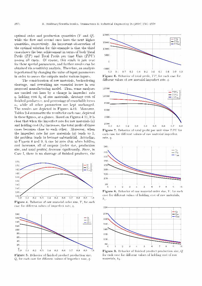
optimal order and production quantities (Y and Q),while the �rst and second ones have the next higherquantities, respectively. An important observation ofthe optimal solution for this example is that the thirdcase shows the best achievement in terms of both TotalPro�t (TP ) and Total Pro�t per time Unit (TPU)among all cases. Of course, this result is just truefor these special parameters, and further results can beobtained via sensitivity analysis. Therefore, an analysisis performed by changing the value of input parametersin order to assess the outputs under various inputs.

The consideration of raw materials, backorderingshortage, and reworking are essential issues in ourproposed manufacturing model. Thus, some analysesare carried out here by a change in imperfect rateq, holding cost h1 of raw materials, shortage cost of�nished products �, and percentage of reworkable items�, while all other parameters are kept unchanged.The results are depicted in Figures 4-19. Moreover,Tables 2-4 summarize the results for each case, depictedin these �gures, at a glance. Based on Figures 4-11, it isclear that when the imperfect rate for raw materials (q)and holding cost (h1) increases, the total pro�t of threecases becomes close to each other. Moreover, whenthe imperfect rate for raw materials (q) tends to 1,the problem tends to become unbene�cial. Accordingto Figures 8 and 9, it can be seen that when holdingcost increases, all of outputs (order size, productionsize, and total pro�ts) decrease signi�cantly. Since, inCase I, there is no shortage of �nished products, the

Figure 4. Behavior of raw material order size, Y , for eachcase for di�erent values of imperfect rate, q.

Figure 5. Behavior of �nished product production size,Q, for each case for di�erent values of imperfect rate, q.

Figure 6. Behavior of total pro�t, TP , for each case fordi�erent values of raw material imperfect rate, q.

Figure 7. Behavior of total pro�t per unit time TPU foreach case for di�erent values of raw material imperfectrate, q.

Figure 8. Behavior of raw material order size, Y , for eachcase for di�erent values of holding cost of raw materials,h1.

Figure 9. Behavior of �nished product production size, Qfor each case for di�erent values of holding cost of rawmaterials, h1.


Figure 10. Behavior of total pro�t, TP , for each case fordi�erent values of holding cost of raw materials, h1.

Figure 11. Behavior of total pro�t per unit time, TPU ,for each case for di�erent values of holding cost of rawmaterials, h1.

Figure 12. Behavior of raw material order size, Y , foreach case for di�erent values of shortage cost, � .

Figure 13. Behavior of �nished product production size,Q, for each case for di�erent values of shortage cost, �.

Figure 14. Behavior of total pro�t, TP , for each case fordi�erent values of shortage cost, �.

Figure 15. Behavior of total pro�t per unit time, TPU ,for each case for di�erent values of shortage cost, �.

Figure 16. Behavior of raw material order size, Y , foreach case for di�erent values of percentage of reworkableitems, �.

Figure 17. Behavior of �nished product production size,Q, for each case for di�erent values of percentage ofreworkable items, �.


Table 2. Results of sensitivity analysis for Case I.

Increase inparameter

Impact on variables and objective functionsY Q TP TPU

q Increases and decreases Decreases Decreases Decreasesh1 Decreases Decreases Decreases Decreases� Unchanged Unchanged Unchanged Unchanged� Decreases Decreases Increases Increases

Table 3. Results of sensitivity analysis for Case II.



q Increases and decreases Decreases Decreases Decreasesh1 Decreases Decreases Decreases Decreases� Decreases Decreases Decreases Decreases� Decreases Decreases Increases Increases

Table 4. Results of sensitivity analysis for Case III.



q Increases and decreases Decreases Decreases Decreasesh1 Decreases Decreases Decreases Decreases� Decreases Decreases Increases and decreases Increases� Decreases Decreases Increases Increases

Figure 18. Behavior of total pro�t, TP , for each case fordi�erent values of percentage of reworkable items, �.

order size, production size, and total pro�ts do notchange in this case. For this case, the raw materialorder size is �xed at YI = 160:5249 (Figure 12), the�nished product production size QI is �xed at 141.2619(Figure 13), the total pro�t TPI is �xed at 13324.3934(Figure 14), and the total pro�t per unit time TPUI is�xed at 9624.9014. Moreover, the total pro�ts in thiscase (TPI and TPUI) are less than those of Case III andgreater than those of Case II. The total pro�t of thesecond case, TPII, starts from 12574.5545 and, then,decreases ultimately, while that of the third case, TPIII,starts from 15894.0332, increases to 16029.0845, andthen decreases. In addition, the total pro�t per unitof the second case, TPUII, starts from 9592.5027 and,then, decreases, while that of the third case, TPUIII,starts from 9713.8521 and, then, increases. According

Figure 19. Behavior of total pro�t per unit time, TPU ,for each case for di�erent values of percentage ofreworkable items, �.

to Figures 16-19, it is clear that when the imperfectrate for raw materials percentage of reworkable items� increases, the total pro�t of the three cases exceedsthe pro�t of each separate case. Generally, the thirdcase is more bene�cial among all the presented cases interms of total pro�t and total pro�t per unit time.

4. Conclusions

In real-world manufacturing systems, there exist im-perfect raw materials and defective products. In orderto address these issues, this paper proposed a manufac-turer system in which raw materials are supplied froman external source, and a �nished product is produced.The structure of this manufacturing planning problem


is based on an EPQ framework. The demand ratefor an item is pre-known and constant; all orderquantities are received instantaneously and all productsare produced gradually via a �nite production rate.Products are entirely consumed when the next orderis commenced. No safety stock is allowed, there is noquantity discount, and ordering/setup cost is �xed perorder/production. In addition to basic assumptions,the existence of a fraction of imperfect raw materialsas well as a defective rate of production system isconsidered. A 100% screening process is carried outupon receiving raw materials, and imperfect items aresold at a discounted price. A number of defectiveproducts are reworkable and have the potential tobecome perfect after the reworking process, whileothers are scrapped items and sold at a lower price.The reworkable �nished products go under a reworkingprocess on the same machine. The defective rate isassumed to be a random variable, resulting in threepossible cases regarding the occurrence of backorderingshortage. Two scenarios for each case are designed,resulting in six total states. The concavity of totalpro�t per unit times is derived for each case separately.Then, the optimal closed-form solution is derived foreach case separately. The proposed manufacturingmodel is illustrated via a numerical example. Anextensive sensitivity analysis is done to assess theimpact of input changes on the outputs variations.

An interesting opportunity for future research isto adopt the proposed model for a more general situa-tion where partial backordering shortage is permitted.Moreover, one may consider a sampling inspectioninstead of 100% inspection, the learning and forgettinge�ects in inspection, or quantity discount as futureresearches of this study.

References

1. Porteus, E. \Optimal lot sizing, process quality im-provement and setup cost reduction", Oper. Res.,34(1), pp. 137-144 (1986).

2. Rosenblatt, M.J. and Lee, H.L. \Economic produc-tion cycles with imperfect production processes", IIETrans., 18(1), pp. 48-55 (1986).

3. Salameh, M.K. and Jaber, M.Y. \Economic produc-tion quantity model for items with imperfect quality",Int. J. Prod. Econ., 64(1-3), pp. 59-64 (2000).

4. C�ardenas-Barr�on, L. \Observation on: economic pro-duction quantity model for items with imperfect qual-ity", Int. J. Prod. Econ., 67(2), p. 201 (2000).

5. Maddah, B. and Jaber, M.Y. \Economic order quan-tity for items with imperfect quality: revisited", Int.J. Prod. Econ., 112(2), pp. 808-815 (2008).

6. Rezaei, J. \Economic order quantity model with back-order for imperfect items", In Proceedings of IEEEinternational Engineering Management Conference,,

11-13 September. St. John's, Newfoundland, Canada,pp. 466-470 (2005).

7. Yu, J.C.P., Wee, H.M., and Chen, J.M. \Optimalordering policy for a deteriorating item with imperfectquality and partial backordering", J. Chin. Inst. Ind.Eng., 22(6), pp. 509-520 (2005).

8. Wee, H.M., Yu, J.C.P., and Wang, K.J. \An integratedproduction-inventory model for deteriorating itemswith imperfect quality and shortage backordering con-siderations", Lect. Notes Comput. Sci. LNCS 3982, pp.885-897 (2006).

9. Papachristos, S. and Konstantaras, I. \Economic or-dering quantity models for items with imperfect qual-ity", Int. J. Prod. Econ., 100(1), pp. 148-154 (2006).

10. Wee, H.M., Yu, J., and Chen, M.C. \Optimal inven-tory model for items with imperfect quality and short-age backordering", Omega, 35(1), pp. 7-11 (2007).

11. Khan, M., Jaber, M.Y., Gui�rida, A.L., andZolfaghari, S. \A review of the extensions of a modi�edEOQ model for imperfect quality items", Int. J. Prod.Econ., 132(1), pp. 1-12 (2011).

12. Wahab, M.I.M., Mamun, S.M.H., and Ongkunaruk, P.\EOQ models for a coordinated two-level internationalsupply chain", Int. J. Prod. Econ., 134(1), pp. 151-158(2011).

13. Konstantaras, I., Skouri, K., and Jaber, M.Y. \Inven-tory models for imperfect quality items with short-ages and learning in inspection", Appl. Math. Model.,36(11), pp. 5334-5343 (2012).

14. Liu, J. and Zheng, H. \Fuzzy economic order quantitymodel with imperfect items, shortages and inspectionerrors", Syst. Eng. Procedia, 4(1), pp. 282-289 (2012).

15. Hsu, J.T. and Hsu, L.F. \An EOQ model withimperfect quality items, inspection errors, shortagebackordering, and sales returns", Int. J. Prod. Econ.,143(1), pp. 162-170 (2013).

16. Rad, M.A., Khoshalhan, F., and Glock, C.H. \Op-timizing inventory and sales decisions in a two-stagesupply chain with imperfect", Comput. Ind. Eng.,74(1), pp. 219-227 (2014).

17. Skouri, K., Konstantaras, I., Lagodimos, A.G., andPapachristos, S. \An EOQ model with backorders andrejection of defective supply batches", Int. J. Prod.Econ., 155(1), pp. 148-154 (2014).

18. Paul, S., Wahab, M.I.M., and Ongkunaruk, P. \Jointreplenishment with imperfect items and price dis-count", Comput. Ind. Eng., 74(1), pp. 179-185 (2014).

19. Hlioui, A., Gharbi, A., and Hajji, A. \Replenishment,production and quality control strategies in three-stagesupply chain", Int. J. Prod. Econ., 166(1), pp. 90-102(2015).

20. Shari�, E., Sobhanallahi, M.A., and Mirzazadeh, A.\An EOQ model for imperfect quality items withpartial backordering under screening errors", CogentEng., 2(1), Article: 994258 (2015).


21. Alamri, A.A., Harris, I., and Syntetos, A.A. \E�cientinventory control for imperfect quality items", Eur. J.Oper. Res., 254(1), pp. 92-104 (2016).

22. Chang, C.T., Cheng, M.C., and Soong, P.Y. \Impactsof inspection errors and trade credits on the economicorder quantity model for items with imperfect quality",Int. J. Syst. Sci.: Oper. Logist., 3(1), pp. 34-48 2016.

23. Rezaei, J. \Economic order quantity and samplinginspection plans for imperfect items", Comput. Ind.Eng., 96(1), pp. 1-7 (2016).

24. Yu, H.F., and Hsu, W.K. \An integrated inventorymodel with immediate return for defective items underunequal-sized shipments", J. Ind. Prod. Eng., 34(1)pp. 70-77 (2017).

25. Sarkar, B. and Saren, S. \Product inspection policy foran imperfect production system with inspection errorsand warranty cost", Eur. J. Oper. Res., 248(1), pp.263-271 (2016).

26. Ongkunaruk, P., Wahab, M.I.M., and Chenc, Y. \Agenetic algorithm for a joint replenishment problemwith resource and shipment constraints and defectiveitems", Int. J. Prod. Econ.m 175(1), pp. 142-152(2016).

27. Taleizadeh, A., Lashgari, M., Akram, R., and Heydari,J. \Imperfect economic production quantity modelwith upstream trade credit periods linked to rawmaterial order quantity and downstream trade creditperiods", Appl. Math. Model., 40(19-20), pp. 8777-8793 (2016).

28. Cheikhrouhou, N., Sarkar, B., Ganguly, B., Malik,A.I., Batista, R., and Lee, Y.H. \Optimization ofsample size and order size in an inventory modelwith quality inspection and return of defective items",Annals of Operations Research, pp. 1-23 (2017) (InPress).

29. Taleizadeh, A.A., and Zamani Dehkordi, N. \Economicorder quantity with partial backordering and samplinginspection", J. of Ind. Eng. Inter., 13(3), pp. 331-345(2017).

30. Mokhtari, H. and Rezvan, M.T. \A single-supplier,multi-buyer, multi-product VMI production-inventorysystem under partial backordering", Operational Re-search, pp. 1-21 (2017) (In Press).

31. Jaber, M.Y., Zanoni, S., and Zavanella, L.E. \Eco-nomic order quantity models for imperfect items withbuy and repair options", Int. J. Prod. Econ., 155(1),pp. 126-131 (2014).

32. Chiu, S.W., Chou, C.L., and Wu, W.K. \Optimizingreplenishment policy in an EPQ based inventory modelwith nonconforming items and breakdown", Econ.Model., 35(1), pp. 330-337 (2013).

33. Bouslah, B., Gharbi, A., and Pellerin, R. \Jointoptimal lot sizing and production control policy in anunreliable and imperfect manufacturing system", Int.J. Prod. Econ., 144(1), pp. 143-156 (2013).

34. Mokhtari, H., Naimi-Sadigh, A., and Salmasnia, A. \Acomputational approach to economic production quan-tity model for perishable products with backorderingshortage and stock-dependent demand", Scientia Iran-ica, 24(4), pp. 2138-2151 (2017).

35. Tayyab, M., and Sarkar, B. \Optimal batch quantityin a cleaner multi-stage lean production system withrandom defective rate", J. of Cleaner Prod., 139(1),pp. 922-934 (2016).

36. Mokhtari, H. \A joint internal production and externalsupplier order lot size optimization under defectivemanufacturing and rework", The International Journalof Advanced Manufacturing Technology, 95(1-4), pp.1039-1058 (2018).

Biography

Hadi Mokhtari is currently an Assistant Professor ofIndustrial Engineering in University of Kashan, Iran.His current research interests include the applicationof operations research and arti�cial intelligence tech-niques to the areas of project scheduling, productionscheduling, and manufacturing supply chains. He alsopublished several papers in international journals suchas Computers and Operations Research, InternationalJournal of Production Research, Applied Soft Com-puting, Neurocomputing, International Journal of Ad-vanced Manufacturing Technology, IEEE Transactionson Engineering Management, and Expert Systems withApplications.

optimal lot size in a manufacturing system with imperfect

Documents