Linköping University Post Print

Optimal placement of UV-based

communications relay nodes

Oleg Burdakov, Patrick Doherty, Kaj Holmberg and Per-Magnus Olsson

N.B.: When citing this work, cite the original article.

The original publication is available at www.springerlink.com:

Oleg Burdakov, Patrick Doherty, Kaj Holmberg and Per-Magnus Olsson, Optimal placement

of UV-based communications relay nodes, 2010, Journal of Global Optimization, (48), 4,

511-531.

http://dx.doi.org/10.1007/s10898-010-9526-8

Copyright: Springer Science Business Media

http://www.springerlink.com/

Postprint available at: Linköping University Electronic Press

http://urn.kb.se/resolve?urn=urn:nbn:se:liu:diva-60067

Optimal placement of UV-based communications relay nodes

Oleg Burdakova,1, Patrick Dohertyb, Kaj Holmberga, Per-Magnus Olssonb

a Department of Mathematics, Linkoping University, SE-581 83 Linkoping, Swedenb Department of Computer and Information Science, Linkoping University, Sweden

Abstract

We consider a constrained optimization problem with mixed integer and realvariables. It models optimal placement of communications relay nodes in the pres-ence of obstacles. This problem is widely encountered, for instance, in robotics,where it is required to survey some target located in one point and convey thegathered information back to a base station located in another point. One or moreunmanned aerial or ground vehicles (UAVs or UGVs) can be used for this purposeas communications relays. The decision variables are the number of unmanned ve-hicles (UVs) and the UV positions. The objective function is assumed to access theplacement quality. We suggest one instance of such a function which is more suitablefor accessing UAV placement. The constraints are determined by, firstly, a free lineof sight requirement for every consecutive pair in the chain and, secondly, a limitedcommunication range. Because of these requirements, our constrained optimizationproblem is a difficult multi-extremal problem for any fixed number of UVs. More-over, the feasible set of real variables is typically disjoint. We present an approachthat allows us to efficiently find a practically acceptable approximation to a globalminimum in the problem of optimal placement of communications relay nodes. Itis based on a spatial discretization with a subsequent reduction to a shortest pathproblem. The case of a restricted number of available UVs is also considered here.We introduce two label correcting algorithms which are able to take advantage ofusing some peculiarities of the resulting restricted shortest path problem. The al-gorithms produce a Pareto solution to the two-objective problem of minimizing thepath cost and the number of hops. We justify their correctness. The presentedresults of numerical 3D experiments show that our algorithms are superior to theconventional Bellman-Ford algorithm tailored to solving this problem.

Keywords: Unmanned vehicles; Global optimization; Hop-restricted shortest paths; Pareto solution; Label

correcting algorithms

1 Introduction

In this paper, we consider the following optimization problem originating from optimalplacement of communications relay nodes.

Given a set X ⊂ Rn and two points s and t in X. One must choose an optimalnumber of points, say k, in the ordered sequence point 1, point 2, . . . , point k. We consider

1Corresponding author. Tel.: +46 13 281473. E-mail address: olbur@mai.liu.se

1

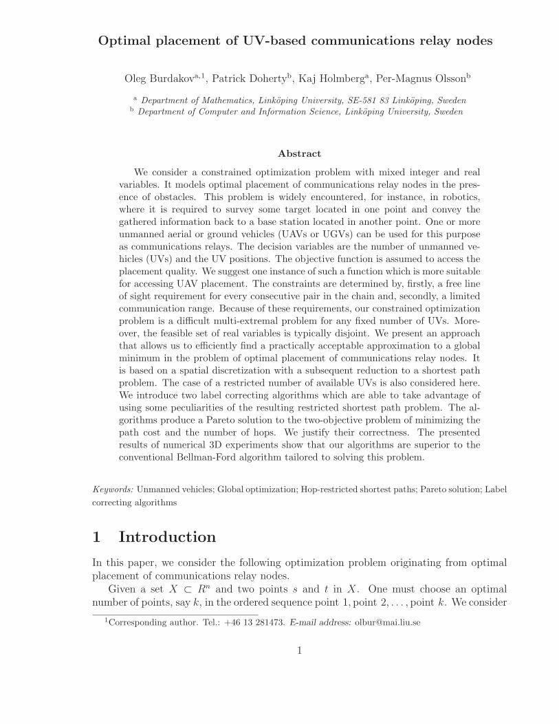
Figure 1: Communications relay

separately the two cases: unrestricted and restricted k. The points are to be placed in Xin an optimal way subject to some constraints. The position of point i, denoted as xi, isassessed by a merit function f(xi), and the sum f(x1) + . . . + f(xk) is to be minimized.The point placement should meet the following requirements, in which we denote x0 = sand xk+1 = t. Any consecutive pair (i, i + 1) in the sequence of points should be placedso that all points of the linear segment

[xi, xi+1] = {x ∈ Rn : x = αxi + (1− α)xi+1, α ∈ [0, 1]}

belong to the set X. Moreover, it is required that the Euclidean distance ‖xi+1−xi‖ doesnot exceed a given radius r > 0.

The described optimization problem can be formulated as follows.

mink∈{0,1,2,...}

F (k), (1)

where the objective function

F (k) = minx1,...,xk∈Rn

k∑

i=1

f(xi)

subject to: [xi, xi+1] ⊂ X, i = 0, 1, . . . , k,‖xi+1 − xi‖ ≤ r, i = 0, 1, . . . , k,x0 = s, xk+1 = t.

(2)

Our interest in this problem is motivated by the communications relay problems com-mon, for instance, in robotics [2, 3, 4, 15, 16, 18, 21, 27, 30, 31, 32, 34], where it is requiredto survey some target located in t and convey the gathered information back to a basestation located in s. One or more unmanned aerial or ground vehicles (UAVs or UGVs)are used as relays. The set X is defined by the terrain within the area of interest. In thecase of UAVs, it is typically the area of interest with removed obstacles which could be,e.g., buildings, hills or mountains. In Fig. 1, X is the white area. It is assumed that theavailable unmanned vehicles (UVs) are equipped with appropriate sensors to survey thetarget and also with means to communicate with each other and the base station. Weconsider here the case when UVs form a chain over which the communication is relayed.

2

The optimal number of UVs, k, and their optimal positions, x1, . . . , xk, are to bedetermined subject to constraints of the following two types.

First, the communication between any consecutive pair of UVs in the chain can onlytake place if there is a free line of sight between them (see Fig. 1). This requirement ismodeled in (2) as [xi, xi+1] ⊂ X.

Second, in any consecutive pair, the UVs are not further away from each other thanthe range of the communication equipment which is characterized by the communicationradius r > 0. As the range of the equipment is limited, it forces the use of intermediaryrelay UVs to convey the information back to the base station if the distance betweenthe target and the base station is longer than the communication range. It is assumed,for simplicity, that the range of the base station communications equipment is the sameas the UAV communication range. The second requirement justifies the presence of theinequality ‖xi+1 − xi‖ ≤ r in (2).

The function f(xi) assessing the UV position xi can be defined in various ways. InSection 2, we suggest to use an obstructed volume as a merit function, whose valueis determined by the local terrain around xi. This is just an example, and it is themerit function which was used in our numerical experiments. In Section 7, we consideralternative forms of the objective function in (2).

Mixed integer programming problems, like (1)–(2), are known to be very difficult tosolve [8, 25]. In our case, the difficulties originate not only from the presence of an integervariable, but mainly because of the multi-extremal nature of the continuous optimizationsub-problem (2). Moreover, the feasible set in (2) is typically disjoint, in which case thereexists at least one couple of feasible points x = (x1, . . . , xk) and x′ = (x′

1, . . . , x′k) in

the kn-dimensional space Rn × . . . × Rn such that any continuous path between themcontains infeasible points. The number of disjoint subsets of the feasible set is in practiceextremely large, and in theory, it may grow exponentially with the number of obstacles.This feature is illustrated in Fig. 1. One can see that there is no feasible continuousvariation of variables that would be able to transform the feasible sequence of pointsx = (x1, . . . , x4) to x′ = (x′

1, . . . , x′4). In this example, there exist a large number of

feasible sequences x = (x1, . . . , x4) which are pair-wise disjoint in this sense.The aim of this paper is to develop an approach that would allow us to efficiently

find a reasonably accurate approximation to a global minimum in the problem of optimalplacement of communications relay nodes. Some practical aspects of using this approachfor positioning UAVs as communication relays for surveillance tasks are discussed in [11].

The main practical significance of our approach is that it allows for finding sucha placement in real time mode almost immediately after the target position becomesavailable. This is achieved by splitting the solution process into the following two stages.

At the presolving stage, an a priori available information about the terrain and thelocation of the base station is processed as completely as possible. Thus, the major com-putational efforts are associated with this stage. This makes vanishing the computationalcost of the second stage, at which the information about the target position is used.

Our approach is based on a discretization of the set X and a reformulation of ourproblem as a shortest path problem (see, e.g., [1]) which is known to be solved in apolynomial time of the number of discretization nodes. To avoid confusion, we shall callit a cheapest path problem, because both path cost and its length (number of hops) will

3

be considered. We introduce a spatial discretization and present a network formulationin Section 3. The discretization as well as the network problem generation and its solvingfor every possible discrete target position can all be done at the presolving stage.

We should emphasize the distinction between our problem and the vehicle path plan-ning problems [13, 24] because one can find some similarities between them. The optimalsolution to problem (1)–(2) can be viewed as a piecewise linear path from s to t. Optimalpaths are of the same shape in some vehicle path planning problems, for instance, inthe Euclidean shortest path problem in polyhedral environment. The principle differenceis that the optimal solution to (1)–(2) has a finite number of jog points. This numberremains bounded from above by a constant with refining the discretization in X, wherethe constant is related to the optimal k in (1). By contrast, the number of jog points inEuclidean shortest paths tends to infinity when the polyhedral approximation of obstaclesis successively refined. Moreover, these jog points belong to the edges of the polyhedra,while in our problem, the jog points located too close to obstacles are not of preferablechoice for placing UAVs.

In practice, the number of communications relay nodes to be optimally placed is oftenrestricted by some number K > 0. This requirement leads to the following reformulationof problem (1)

mink∈{0,1,...,K}

F (k). (3)

In our network formulation considered in Section 4, this problem corresponds to acheapest path problem with restricted number of hops. In practice, it may be necessaryto solve this problem repeatedly for every new target position and number of availableUVs. Therefore, in Section 4, we address also the more general problem of finding optimalplacement of a limited number of communications relay nodes for every possible discretetarget position. It is reduced to the all hops optimal path (AHOP) problem [23]. Theconsideration of this more general problem allows us to move the major computationalburden on the mentioned presolving stage.

The conventional Bellman-Ford algorithm is widely used for finding a tree of unre-stricted cheapest paths. It has been noticed, e.g., in [1, 25] that the labels generated bythis algorithm contain all AHOP solutions. In Section 5, we present the Bellman-Fordalgorithm tailored in [25] to solving AHOP problems. We then introduce two new andconsiderably more efficient label correcting algorithms for solving the same problems andprove their correctness. They can be viewed as modifications of the algorithm of [25].Their efficiency results from using some peculiarities of the UV-based communicationsrelay problem. The important feature of these algorithms is that for each possible targetposition they produce a Pareto solution. It is an optimal solution to the multi-criteriaproblem of minimizing both the path cost and the number of hops. We are interested inminimizing the number of hops because this minimizes the number of UVs required formaintaining the communications relay.

Results of our numerical experiments are presented in Section 6. The consideredtest problems originate from UAV applications with various 3D terrain topologies. Thenumber of discretization points varies from medium to very large. The experiments showthat our algorithms are superior to the Bellman-Ford-type algorithm of [25].

In Section 7, we draw conclusions and discuss future work.

4

Figure 2: The 500-gram LinkMAV Micro Aerial Vehicle.

Figure 3: Visible and invisible parts of a ball centered in xi

2 Use of obstructed volume for assessing UAV

position

In the applications that the authors are dealing with, UAVs are used as communicationrelays. Some of them are very light, like the one in Fig. 2. It is important to position theUAVs safely far away from obstacles for many reasons. For instance, the positions of UAVsmay be affected by strong winds or by a necessity to make limited moves caused by limitedpurposeful moves of the surveying UAV. In all these cases, uninterrupted communicationshould be maintained. This requires a sufficiently large free-of-obstacles room aroundeach of the UAVs. In a sense, this means that the UAVs should be better centered withrespect to the surrounding obstacles. Moreover, the better centered positions are oftenrelated to the better communication quality. The same position property is important forthe surveying UAV also because the target is typically not located in the correspondinggrid point.

In the line of this, we suggest to define the function f(xi) assessing the UAV positionxi, for example, as the volume of obstacles and their ‘shade’ within the ball {x ∈ R3 :‖x − xi‖ ≤ r′}. Here the radius r′ may be either the same as, or different from, thecommunication radius r. In other words, f(xi) is the volume of the part of the ball whichis invisible from the point xi (see Fig. 3). Obviously, f(xi) = 0 means that there is noobstructed volume within the ball, and the maximal value of f(xi) is equal to the volume

5

Figure 4: Obstructed volume for three UAV positions

of the ball. Our desire to find a UAV location xi, which makes the obstructed volumef(xi) as small as possible, implies maximization of the visible volume of the sphere.

Our choice of f(xi) is closely related to the concept of an isovist introduced in [39]. Anisovist, or viewshed, is the area in a spatial environment directly visible from a given point.In our applications this area is restricted by a ball. Isovist is widely used in architecturalstudies, geoinformation science, computational geometry and computer graphics. It issuccessfully applied in the problems of line of sight communication, VLSI circuits design,robot and sensor network design, motion planning, architectural and urban planning,computer games etc. Since some of them admit problem formulations similar to (1)–(2),they can be viewed as potential areas for extending the approach presented in this paper.

There exist efficient algorithms that can be used in our applications for computing theobstructed volume f(xi) (see, e.g., [7, 19, 28, 36, 40]).

With our suggested choice of f(xi), positions xi well distant from obstacles are favoredover those which are closer to obstacles. This ensures that the better centered points are ofpreferable choice for placing UAVs. Fig. 4 presents an example in which f(xi) > f(x′

i) >f(x′′

i ), and therefore, the position x′′i is the most preferable among the considered three

alternatives. In what follows, we do not use any specific feature of f(xi) and assume thatit is just a given function.

3 Spatial discretization and network formulation

For the purpose of solving problem (1)–(2) approximately, let us restrict our choice ofplacing x1, . . . , xk by a discrete set of points D ⊂ Rn. This can be done, for instance, byintroducing a grid in the area of interest. Then the minimization in (2) is performed overx1, . . . , xk ∈ D.

The introduced discretization, in itself, does not make any considerable simplificationof problem (1)–(2). Since it still looks intractable, we will construct a network by takingadvantage of using such characteristic features of problem (2) as the additive objectivefunction and chain-type constraints. Our network, i.e. a weighted directed graph, will beconstructed on the base of an undirected graph.

To formalize our network problem, let us regard the discrete points D ∩X as nodes.We denote the set of nodes by N . For simplicity, the same notation will sometimes beused for both points and nodes.

6

Figure 5: Spatial discretization (the set D ∩ X is presented by the dots ◦ and •). Thepoints x′ and x′′ are intervisible and meet the limited distance requirement. Nodes • areadjacent to x′ in the visibility graph.

Let the set E ⊂ N × N be composed of the couples x′, x′′ ∈ D ∩ X which both areintervisible, i.e. [x′, x′′] ⊂ X, and meet the limited distance requirement ‖x′ − x′′‖ ≤ r.The set of nodes N and the set of undirected edges E define the visibility graph G = (N,E)(see Fig. 5).

Using the available visibility graph G, one can easily answer the practical questionabout the minimal number of UVs required to establish a relay-type communication linkbetween the base and the terminal UV for the given target location. The breadth-firstsearch [14] is ideally suited for this purpose, because its computational complexity growslinearly with the number of edges.

Visibility graphs are widely used in the areas listed in Section 1 in connection withthe notion of isovist and viewshed. For constructing visibility graphs, there exist notonly efficient computational algorithms [7, 19, 22, 28, 36, 40] and software [29], but alsohardware accelerators [35].

Note that the number of uniformly distributed grid points, which are within the dis-tance r′ from xi and invisible for xi, is proportional to the obstructed volume. Therefore,this number can be used instead of the obstructed volume to define f(xi). It can be cal-culated for a given visibility graph G by subtracting the corresponding node degree, i.e.the number of nodes adjacent to xi, from the maximum possible number of grid pointsin a sphere of the radius r′. This way of defining f(xi) can be extended to the case ofnonuniformly distributed grid points.

Assuming that s, t ∈ N , the optimal placing of communications relay nodes is thenreduced to finding in this graph a path between the nodes s and t which minimizes thesum f(x1)+. . .+f(xk). Notice that each term in this objective function is associated withthe corresponding node. Since this observation does not allow us yet to apply directlyany of the conventional network optimization methods [1, 9] to solving this problem, wewill introduce directed edges and define their costs.

We suggest to change from the undirected graph G to a directed one G as follows.

7

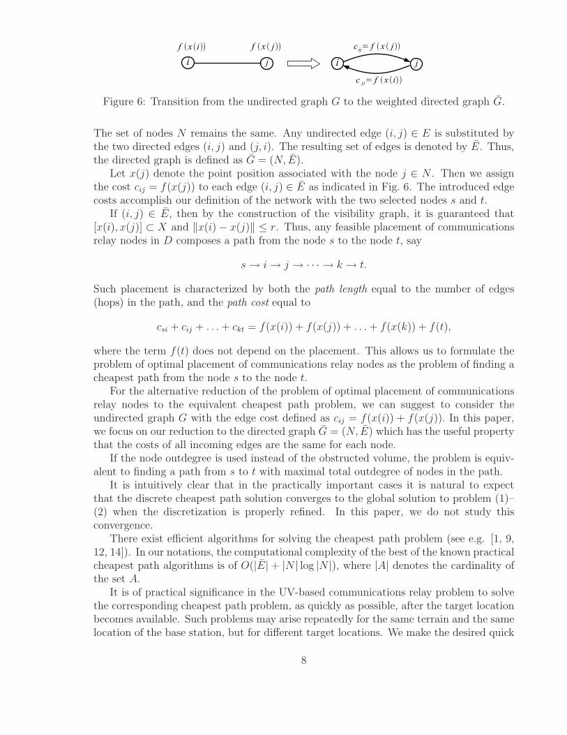
Figure 6: Transition from the undirected graph G to the weighted directed graph G.

The set of nodes N remains the same. Any undirected edge (i, j) ∈ E is substituted bythe two directed edges (i, j) and (j, i). The resulting set of edges is denoted by E. Thus,the directed graph is defined as G = (N, E).

Let x(j) denote the point position associated with the node j ∈ N . Then we assignthe cost cij = f(x(j)) to each edge (i, j) ∈ E as indicated in Fig. 6. The introduced edgecosts accomplish our definition of the network with the two selected nodes s and t.

If (i, j) ∈ E, then by the construction of the visibility graph, it is guaranteed that[x(i), x(j)] ⊂ X and ‖x(i)− x(j)‖ ≤ r. Thus, any feasible placement of communicationsrelay nodes in D composes a path from the node s to the node t, say

s→ i→ j → · · · → k → t.

Such placement is characterized by both the path length equal to the number of edges(hops) in the path, and the path cost equal to

csi + cij + . . . + ckt = f(x(i)) + f(x(j)) + . . . + f(x(k)) + f(t),

where the term f(t) does not depend on the placement. This allows us to formulate theproblem of optimal placement of communications relay nodes as the problem of finding acheapest path from the node s to the node t.

For the alternative reduction of the problem of optimal placement of communicationsrelay nodes to the equivalent cheapest path problem, we can suggest to consider theundirected graph G with the edge cost defined as cij = f(x(i)) + f(x(j)). In this paper,we focus on our reduction to the directed graph G = (N, E) which has the useful propertythat the costs of all incoming edges are the same for each node.

If the node outdegree is used instead of the obstructed volume, the problem is equiv-alent to finding a path from s to t with maximal total outdegree of nodes in the path.

It is intuitively clear that in the practically important cases it is natural to expectthat the discrete cheapest path solution converges to the global solution to problem (1)–(2) when the discretization is properly refined. In this paper, we do not study thisconvergence.

There exist efficient algorithms for solving the cheapest path problem (see e.g. [1, 9,12, 14]). In our notations, the computational complexity of the best of the known practicalcheapest path algorithms is of O(|E| + |N | log |N |), where |A| denotes the cardinality ofthe set A.

It is of practical significance in the UV-based communications relay problem to solvethe corresponding cheapest path problem, as quickly as possible, after the target locationbecomes available. Such problems may arise repeatedly for the same terrain and the samelocation of the base station, but for different target locations. We make the desired quick

8

solving achievable by presolving the problem in advance. For this purpose, we take intoaccount as much of the a priori available information as possible.

At the presolving stage, we suggest to discretize the area of interest, construct thevisibility graph, and then solve the resulting single-source cheapest path problem [1, 9, 14],whose solution is a tree of cheapest paths from s to each node in N . The cheapest pathtree composes a special kind of communication map which for each node contains thelocation of its immediate predecessor in a cheapest path from s to this node.

At the stage when the location of the target becomes available, an optimal placementof relay nodes can be very quickly retrieved from the communication map. The numberof required arithmetic operations is proportional to the optimal number of relay nodes.It is vanishing in comparison with O(|E|+ |N | log |N |), the best known complexity of thealgorithms that can be used at the presolving stage.

4 Restricted number of relay nodes

In this section, we consider problem (2)–(3) assuming that the maximal number of relaynodes K is given. After generating the network as described in Section 3, this problemis reduced to the cheapest path problem with a restricted number of nodes in path, orequivalently, with a restricted number of edges (hops). In the latter problem, K + 1 isthe maximal number of edges in the optimal path to be found.

In relation to the hop-restricted cheapest path problem, we should mention here theweight-restricted cheapest path problem [17], which can be formulated as follows. Givena directed graph with edge costs cij, edge weights wij and the upper limit K for the pathweight, find a cheapest path from s to t whose weight does not exceed K. It is knownto be an NP-hard problem, however it can be solved in pseudopolynomial time. In [17],one can find an overview of the existing algorithms. Our hop-restricted cheapest pathproblem is a special case in which wij = 1 for all edges, and it can be solved in polynomialtime.

We call a path k-restricted if it consists of at most k edges. We will consider herethe all hops optimal path (AHOP) problem [23]. It consists in finding a k-restrictedcheapest path from a selected node s to all j ∈ N for each k = 1, 2, . . .. Note that in thementioned hop-restricted cheapest path problem the value of k is fixed. The reasoning inthis section does not take into account any information about the UV origination of thegraph G = (N, E). The only assumption is that G has no cycle of negative cost.

Let d(j) stand for the depth of node j with respect to node s, i.e. d(j) is the minimalnumber of edges over all paths from s to j. If there is no path from s to j, we defined(j) =∞. We denote the maximal depth over all j ∈ N reachable from s by

kmax = max{d(j) : j ∈ N, d(j) <∞}.

The value kmax − 1 can be interpreted as the minimal number of UVs which would bedefinitely sufficient to survey a target at any discrete position, not necessarily in theoptimal way.

The notation d∗(j) will be used for the minimal number of edges (hops) over allcheapest paths from s to j. We call a cheapest path tree least-hops if, for each j ∈ N , the

9

length of the path in this tree from s to each j is minimal, i.e. it is equal to d∗(j). Letk∗

max denote the height of a least-hops cheapest path tree, which means that

k∗max = max{d∗(j) : j ∈ N, d∗(j) <∞}.

The value k∗max − 1 can be interpreted as the minimal number of UVs sufficient for the

optimal surveillance of a target at any discrete position.Since the set of cheapest paths is a subset of all paths, we have

d(j) ≤ d∗(j), ∀j ∈ N,

and kmax ≤ k∗max.

We say that an AHOP problem admits a trivial solution if

d(j) = d∗(j), ∀j ∈ N.

Then kmax = k∗max. In our UV applications, this case means that, for each target position,

there exists an optimal placement of the relay nodes with the minimum possible numberof UVs. In [10], we present a sufficient condition for the AHOP problem to admit a trivialsolution. This condition is formulated in terms of the edge costs cij.

The notations g∗k(j) and g∗(j) will be used for the cost of, respectively, a k-restricted

and standard (unrestricted) cheapest path from s to j. If 0 ≤ k < d(j), there is nok-restricted path from s to j, and in this case we define g∗

k(j) = +∞.Obviously,

g∗0(j) ≥ g∗

1(j) ≥ . . . ≥ g∗k(j) ≥ g∗

k+1(j) ≥ . . . (4)

Moreover, g∗k(j) ≥ g∗(j) for all k ≥ 0. More detailed relations between g∗

k(j) and g∗(j)are presented below by Lemma 1.

Letj− = {i ∈ N : (i, j) ∈ E}, j+ = {i ∈ N : (j, i) ∈ E}

denote the sets of all immediate predecessors and successors of node j ∈ N , respectively.In this notation, the optimality conditions for the AHOP problem can be written (see,e.g. [25]) in the form of the recursion relation

g∗k(j) = min{g∗

k−1(j), mini∈j−{g∗

k−1(i) + cij}} (5)

valid for any j ∈ N and k ≥ 0. It can be viewed as a Bellman-type recurrence equation[1, 6, 9, 20].

The optimality conditions allows us to formulate the following lemma. It will be usedfor proving the correctness of the algorithms presented in the next section.

Lemma 1 Let a weighted directed graph G = (N, E) with source s contain no negativecycles. Then the optimal solution to the AHOP problem has the following structure.

a) If, for some i, j ∈ N and k such that (i, j) ∈ E and 2 ≤ k ≤ k∗max, the relations

g∗k−2(i) = g∗

k−1(i) and g∗k−1(j) > g∗

k(j) hold, then g∗k−1(i) + cij > g∗

k(j).

b) g∗k(j) > g∗(j) iff k < d∗(j).

10

c) g∗k(j) = g∗(j) iff k ≥ d∗(j).

Proof. By optimality conditions (5) and the assumptions in a), we obtain the relations

g∗k(j) < g∗

k−1(j) ≤ g∗k−2(i) + cij = g∗

k−1(i) + cij,

which prove statement a).Statements b) and c) simply follow from the fact that d∗(j) is the minimal number of

edges for all unrestricted cheapest paths from s to j, and g∗(j) is the cost of such paths.Indeed, if the number of edges in a path is less than d∗(j), the path cost must be largerthan g∗(j). Moreover, it is obvious that for k ≥ d∗(j) there is no k-restricted path whichis cheaper than g∗(j), while there exists a path of the cost g∗(j) and the length d∗(j).

If an AHOP problem admits a trivial solution, then for all j ∈ N and k ≥ 0, byLemma 1, we have

gk(j) =

{

+∞, if 0 ≤ k < d∗(j)g∗(j), if k ≥ d∗(j)

.

5 AHOP algorithms

The following successive approximation algorithm introduced by Lawler [25] is based onthe recursion relation (5), and it extracts the AHOP solutions from the labels generatedby the conventional Bellman-Ford algorithm.

Algorithm 1.

1 for each i ∈ N \ {s} do

2 g0(i)← +∞3 g0(s)← 04 for k = 1, 2, . . . , |N | − 1 do

5 for each j ∈ N do

6 gk(j)← gk−1(j)7 for each i ∈ N do

8 for each j ∈ i+ do

9 if gk−1(i) + cij < gk(j) then

10 gk(j)← gk−1(i) + cij

At iteration k, Algorithm 1 produces implicitly, for each node j ∈ N , a k-restrictedpath from s to j of the cost gk(j), which is an upper estimate for g∗

k(j). Whenever the labelgk(j) is improved, the path is updated. At the end of the k-th iteration, the algorithmgenerates

gk(j) = g∗k(j), ∀j ∈ N. (6)

This statement is justified, e.g., in [1, p. 142].We introduce here two modifications of Algorithm 1 which are able to take advantage

of using some characteristic features of the AHOP problems originating from our UV-based applications. The modifications are built upon the properties of the optimal AHOPsolutions presented by Lemma 1.

11

The computational complexity of Algorithm 1 is O(|N ||E|) (see e.g. [1]). This estimateis justified by the necessity of performing |N | − 1 iterations of the for loop in lines 4-10,which contains the for loop in lines 7-10 to be performed for all edges.

We observe that iteration k = k∗max results in gk(j) = g∗(j) for all j ∈ N . This

means that gk(j) has attained its minimal value and would not change at the subsequentiterations. Therefore, Algorithm 1 can be terminated after this iteration.

Clearly k∗max < |N |. It should be emphasized that, in the practical placement of

communications relay nodes, the value of k∗max mostly depends on the terrain topology.

For given area of interest, k∗max does not change much with the increasing number of

discrete points |N |, if it changes at all. It is natural to expect for properly refiningdiscretization that k∗

max−1 tends to the maximal value of k(t) over all possible continuoustarget positions t, where k(t) is an optimal solution to problem (1)–(2). In other words,k∗

max tends to the minimal number of UVs which would be definitely sufficient for theoptimal surveillance of a target at any position. For our applications, it is typical that

k∗max << |N |. (7)

This observation is taken into account in Algorithm 2 (presented below), which can beviewed as a modification of Algorithm 1.

Another observation is based on Lemma 1a). It states that if gk−1(i) did not changeat iteration k − 1, then gk−1(i) + cij is not able to improve the value of gk(j), i.e. in thiscase, line 10 of Algorithm 1 is not performed for node i at iteration k. Therefore, the for

loop in lines 8-10 can be restricted to only those edges (i, j) ∈ E which begin in nodes ithat compose the set

Vk = {i ∈ N : gk−1(i) 6= gk−2(i)}.

Algorithm 2 gains the most benefit from using this observation.In Algorithm 2, the label g(j) takes the same values at iteration k as gk(j) in Algo-

rithm 1. If g(j) changes at the k-th iteration, we set gk(j) ← g(j), and if not, no labelgk(j) is assigned to node j at iteration k.

Algorithm 2 has an extra feature. At iteration k, it produces for each node j ∈ N itsimmediate predecessor p(j) in the k-restricted path from s to j. The cost of this pathg(j) gives an upper estimate for g∗

k(j). At the end of the k-th iteration of Algorithm 2,the equality

g(j) = g∗k(j), ∀j ∈ N (8)

similar to (6) holds, and p(j) is the immediate predecessor of node j in the implicitlyproduced k-restricted cheapest path from s to j. The cost of this path is equal to g∗

k(j).It will be explained below how to retrieve this path from the available list of predecessorsp1(·), . . . , pk(·). The mentioned feature was not introduced in Algorithm 1, because wewish to simplify its formal presentation and to focus on its modifications.

As a result of the k-th iteration of Algorithm 2, the set Vk+1 is composed of thosenodes j ∈ N for which a cheaper path from s to j has been found at this iteration, i.e.g∗

k(j) < g∗k−1(j). Only these nodes are used at the next iteration to possibly improve the

value of gk+1 for their immediate successors. This allows Algorithm 2 to reduce in practicethe total number of elementary operations, although the worst-case estimate remains thesame as for Algorithm 1, namely, O(|N | |E|).

12

The outlined algorithm can be formally presented as follows.

Algorithm 2.

1 for each i ∈ N \ {s} do

2 g(i)← +∞3 g(s)← 0, g0(s)← g(s), p0(s)← nil, V1 ← {s}4 for k = 1, 2, . . . while |Vk| 6= 0 do

5 Vk+1 ← ∅6 for each i ∈ Vk do

7 for each j ∈ i+ do

8 if gk−1(i) + cij < g(j) then

9 g(j)← gk−1(i) + cij, p(j)← i, Vk+1 ← Vk+1 ∪ {j}10 for each j ∈ Vk+1 do

11 gk(j)← g(j), pk(j)← p(j)

Algorithm 2 returns a collection of triples {k, gk(j), pk(j)} produced for each nodej ∈ N . We call them kgp-triples. The output of Algorithm 2 for node j may not containkgp-triples for some values of k. In fact, in our applications, such collections are typicallyvery sparse - just one or a few kgp-triples per one node. Recall that, in (4), the sequenceof non-increasing values of g∗

k(j) may remain the same for some number of the consecutivevalues of k. The kgp-triples are produced by Algorithm 2 only for those values of k whichare minimal in such series of equal values of g∗

k(j). Therefore, in order to find the valueof a, possibly, missing triple {k, gk(j), pk(j)}, it is necessary to find the largest k′ ≤ k forwhich a kgp-triple {k′, gk′(j), pk′(j)} exists. Then the desired values are gk(j) = gk′(j) andpk(j) = pk′(j). If such k′ does not exist, then gk(j) = +∞ and pk(j) = nil. A k-restrictedcheapest path from s to j can be retrieved from the available kgp-triples as follows. Weset jk′ = j, and then recursively find

jk′−1 = pk′(jk′), jk′−2 = pk′−1(jk′−1), . . . , j0 = p1(j1), (9)

where j0 = s.The main properties of Algorithm 2 are summarized in the following theorem.

Theorem 2 Let Algorithm 2 be run on a weighted directed graph G = (N, E) with sources. Assume that this graph contains no negative cycles. Then after k iterations of thefor loop in lines 4-11, equation (8) holds. Moreover, the generated kgp-triples correctlydefine, for each node j ∈ N , a path of the optimal cost g∗

k(j). The length of this path isminimal over all cheapest k-restricted paths from s to j, if such paths exist, and it is equalto the largest k′ ≤ k for which a triple {k′, gk′(j), pk′(j)} exists. Algorithm 2 terminatesin k = k∗

max + 1 iterations.

Proof. Denote V ∗1 = {s} and

V ∗k = {i ∈ N : g∗

k−1(i) 6= g∗k−2(i)} (10)

for k ≥ 2. By Lemma 1, the optimality conditions (5) can be written as

g∗k(j) = min{g∗

k−1(j), mini∈j−∩V ∗

k

{g∗k−1(i) + cij}}. (11)

13

Then it can be easily shown, by induction in k = 1, 2, . . . , k∗max, that after iteration k,

equation (8) holds and Vk = V ∗k . By the definition of k∗

max, V ∗k 6= ∅ for these values of k.

Therefore, Algorithm 2 can not terminate before iteration k = k∗max + 1. By Lemma 1

and equation (8), at the end of iteration k = k∗max we have

g(j) = g∗(j), ∀j ∈ N.

At the next iteration, none of these values of g(j) can be decreased. Therefore, Vk∗

max+2 = ∅and Algorithm 2 terminates after iteration k = k∗

max + 1.By the assumption of the theorem, a triple

{k′, gk′(jk′), pk′(jk′)}

was generated by Algorithm 2 for jk′ = j. Then pk′(jk′) ∈ V ∗k′ . This, by definition (10),

ensures that the triple

{k′ − 1, gk′−1(pk′(jk′)), pk′−1(pk(jk′))}

exists. By reasoning recursively in the same way, we can prove the correctness of therecursive procedure defined by (9). Since V ∗

1 = {s}, we have j0 = s. Thus, (9) defines apath from s to j with the path cost g∗

k(j). Then it can be easily shown, by induction ink, that the length of this path is minimal over all cheapest k-restricted paths from s toj.

Consider the two-criteria optimization problem in which both the path cost and itslength (the number of hops) are to be minimized for each node. Theorem 2 implies thatAlgorithm 2 generates a Pareto optimal solution to this problem. Algorithm 1 could alsoproduce a Pareto optimal solution if to modify it properly.

Observe that the major computational burden of Algorithms 1 and 2 is associatedwith the execution of lines 9-10 and 8-9, respectively.

In Algorithm 1, lines 9-10 are executed approximately |E| |N | times, because eachedge (i, j) is used only once for each k.

Similar calculations show that lines 8-9 of Algorithm 2 are executed at most k∗max|E|

times. In the problems for which (7) holds, this very rough estimate is much better than|N | |E|. To continue with a more refined analysis of the computational burden, we denote:

Ek = {(i, j) ∈ E : i ∈ Vk, j ∈ i+},

|Emax| = max{|Ek| : 1 ≤ k ≤ k∗max}.

Then it is not difficult to verify that the number of elementary operations of Algorithm 2grows in proportion to the value

k∗

max∑

k=1

|Ek|.

Since this estimate is bounded above by k∗max|Emax|, it is typically well below k∗

max|E| forour applied problems, in which |Ek| is far less than |E|.

14

Our further progress in reducing the number of elementary operations is related withthe use of the cheapest path tree. If the edge costs are non-negative, this tree can beproduced, for instance, by Dijkstra’s algorithm. Its computational complexity is O(|E|+|N | log |N |). We need the cheapest path tree to possess the least-hops property. This extraproperty can be assured by a simple modification of the algorithms producing cheapestpath trees. For this purpose, not only a path cost should be associated with each node,but also the length of this path. The currently best path can be improved not only whena candidate path has a smaller cost, but also when its length is smaller while the cost isthe same as the currently best one (for the formal presentation of this modification, see[10]).

Let p∗(j) denote the immediate predecessor of node j ∈ N in a given least-hopscheapest path tree. Hereafter we assume that such a tree is available. More specifically,not only the number k∗

max and the kgp-triples

{d∗(j), g∗(j), p∗(j)}, j ∈ N, (12)

are assumed to be available, but also the sets

N∗k = {j ∈ N : d∗(j) = k}, k = 0, 1, . . . , k∗

max. (13)

All these sets can be generated for a given tree in a linear time of the number of nodes|N |.

We observe that, for any node j ∈ N , the inequality in line 9 of Algorithm 2 obviouslyholds at each iteration k > d∗(j). Therefore, it is not necessary to check this inequalityat any of these iterations. Moreover, if the value of g∗(j) is available for a node j, it isnatural to skip the execution of lines 9-10 for this node at the iteration k = d∗(j).

For any node j ∈ N , we can avoid the unnecessary execution of these lines at iterationsk ≥ d∗(j) by excluding at iteration k = d∗(j) node j from all the sets i+ such that i ∈ j−.This is the key observation which allows us to efficiently exploit the available least-hopscheapest path tree. It is implemented in the following algorithm.

Algorithm 3.

1 for each i ∈ N \ {s} do

2 g(i)← +∞3 V0 ← ∅4 for k = 0, 1, . . . , k∗

max − 1 do

5 for each j ∈ N∗k do

6 for each i ∈ j− do

7 i+ ← i+ \ {j}8 Vk+1 ← ∅9 for each i ∈ Vk do

10 for each j ∈ i+ do

11 if gk−1(i) + cij < g(j) then

12 g(j)← gk−1(i) + cij, p(j)← i, Vk+1 ← Vk+1 ∪ {j}13 for each j ∈ Vk+1 do

14 gk(j)← g(j), pk(j)← p(j)15 Vk+1 ← Vk+1 ∪N∗

k

15

Before this algorithm is executed, the sets N∗k and a least-hops cheapest path tree

must be determined.The main properties of Algorithm 3 can be summarized in the same way as it has

been done in Theorem 2 for Algorithm 2. We skip it, because the difference in theirformulations and proofs are pretty obvious. It can be easily seen also that the totalnumber of elementary operations is less for Algorithm 3 than for Algorithm 2. Thisderives from the fact that i+ in the set of edges associated with the for loops in lines6-7 and 10-12 of Algorithm 3 is a subset of the set of edges which are used at the sameiteration of Algorithm 2.

Line 7 of Algorithm 3 is equivalent to the exclusion of the edge (i, j) from the setE. Since this operation is done at most once for each edge, the computational burdenassociated with lines 5-7 grows linearly with the number of edges |E|.

If in our UV applications the terrain topology is not too complicated, the correspondingAHOP problem may admit a trivial solution. In this case, at each iteration of Algorithm 3we have i+ = ∅ in line 7, Vk+1 = ∅ in line 13, and Vk+1 = N∗

k in line 15. It is themost favorable case for Algorithm 3, because the total number of elementary operationsassociated with lines 8-15 grows linearly with |N |.

In general, the smaller the difference is between the node distances d∗k(j) and dk(j),

the lower the computational burden of Algorithm 3.

6 Implementation issues and numerical experiments

Here we consider test problems originating from optimal placement of UAV-based commu-nications relay nodes. Such problems are characterized by relation (7). Another featureof these problems is that the edge costs are non-negative.

Our test problems cover various 3D terrain topologies. Each row in Table 1 refers toone test case. The first five columns present some features of the generated directed graphG = (N, E). Column ‘outdegree’ specifies the min/max/average node outdegree.

In column ‘%kgp > 1’, the percentage of nodes j with d∗(j) > d(j) is indicated.Such nodes have more than one kgp-triple. Zero value means that the corresponding testproblem admits a trivial solution. To increase the portion of nodes with d∗(j) > d(j),we modified some of the test problems by artificially increasing f(x(i)) for one arbitraryselected node i which was a successor of node s in the original cheapest path tree. Theartificially modified problems are marked by star in the first column of Table 1.

One can see that the number of discretization points varies from medium to very large.In the largest test problem, the area of interest is of the size 1000m× 1000m× 60m, thediscretization step is 10m, and the communication radius r = 100m. The obstacles inthis problem model an urban environment.

In the previous section, it was mentioned that Algorithm 1 can be terminated afteriteration k = k∗

max. Since the value of k∗max is not available, one can terminate Algorithm 1

as soon asgk(j) = gk−1(j), ∀j ∈ N,

results from iteration k.

16

This idea is widely used in implementations of the Bellman-Ford algorithm. Here itwas implemented by setting flag ← true at the very beginning of iteration k, and if theinequality in line 9 of Algorithm 1 holds at least once, we set flag ← false. Then thefor loop in lines 4-10 is terminated as soon as flag = true at the very end of iteration k.We shall refer to this modification as Algorithm 1′.

This simple idea provides a speedup factor of about |N |/k∗max, which is approximately

103 in the largest of the test examples considered below. Due to (7), the speedup factorgrows linearly with |N |. One should bear this in mind, when we compare our Algorithms2 and 3 with Algorithm 1′, which is actually the conventional Bellman-Ford algorithmtailored to solving our UV-related problems.

We were using C++ for implementing our algorithms. Algorithm 2 was implementedwith no change.

Our implementation of Algorithm 3 was based on the following observation. One canskip the for loop in lines 5-7 of Algorithm 3 if line 10 is changed as follows

10 for each j ∈ i+ such that d∗(j) > k do

We shall refer to this implementation as Algorithm 3′. More sophisticated implemen-tations of our algorithms and their detailed comparison will be the main subject of aseparate paper.

Algorithm 3′ requires that k∗max and the part of kgp-triples presented by (12) are

available. They are produced by Dijkstra’s algorithm modified in the way outlined in theprevious section. Dijkstra’s algorithm was implemented with the use of the standard heapalgorithms available in the C++ template library.

The sets N∗k (13) are also required to be available for Algorithm 3′. They are produced

at the preprocessing stage by sorting the nodes j ∈ N in the increasing order of d∗(j) withsubsequent identification of the segments N∗

1 , N∗2 , . . . in the obtained sequence of sorted

nodes.The numerical results presented here were produced on a PC running under Windows

Vista with an Intel Core 2 Duo processor (2.4 GHz, 2GB RAM). Only one core wasinvolved in the computational process. The CPU time was measured in millisecondsaveraged over 1000 runs. We used the O2 optimization flag in the Microsoft VisualStudio 2008 C++ compiler.

The CPU time of running Algorithms 1′, 2, 3′ and Dijkstra’s algorithm are presented bythe corresponding columns in Table 1. We shall refer to the combination of Algorithm 3′,Dijkstra’s and preprocessing algorithms as the combined Algorithm 3′. The run time ofthe preprocessing algorithm is not reported here because it was less than 1% of the runtime of the combined Algorithm 3′ presented by the last column.

17

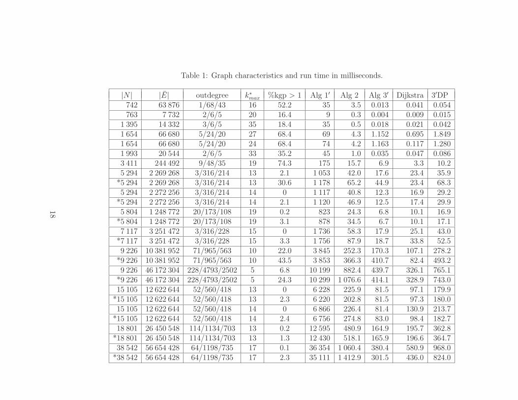
Table 1: Graph characteristics and run time in milliseconds.

|N | |E| outdegree k∗max %kgp > 1 Alg 1′ Alg 2 Alg 3′ Dijkstra 3′DP

742 63 876 1/68/43 16 52.2 35 3.5 0.013 0.041 0.054763 7 732 2/6/5 20 16.4 9 0.3 0.004 0.009 0.015

1 395 14 332 3/6/5 35 18.4 35 0.5 0.018 0.021 0.0421 654 66 680 5/24/20 27 68.4 69 4.3 1.152 0.695 1.8491 654 66 680 5/24/20 24 68.4 74 4.2 1.163 0.117 1.2801 993 20 544 2/6/5 33 35.2 45 1.0 0.035 0.047 0.0863 411 244 492 9/48/35 19 74.3 175 15.7 6.9 3.3 10.25 294 2 269 268 3/316/214 13 2.1 1 053 42.0 17.6 23.4 35.9

*5 294 2 269 268 3/316/214 13 30.6 1 178 65.2 44.9 23.4 68.35 294 2 272 256 3/316/214 14 0 1 117 40.8 12.3 16.9 29.2

*5 294 2 272 256 3/316/214 14 2.1 1 120 46.9 12.5 17.4 29.95 804 1 248 772 20/173/108 19 0.2 823 24.3 6.8 10.1 16.9

*5 804 1 248 772 20/173/108 19 3.1 878 34.5 6.7 10.1 17.17 117 3 251 472 3/316/228 15 0 1 736 58.3 17.9 25.1 43.0

*7 117 3 251 472 3/316/228 15 3.3 1 756 87.9 18.7 33.8 52.59 226 10 381 952 71/965/563 10 22.0 3 845 252.3 170.3 107.1 278.2

*9 226 10 381 952 71/965/563 10 43.5 3 853 366.3 410.7 82.4 493.29 226 46 172 304 228/4793/2502 5 6.8 10 199 882.4 439.7 326.1 765.1

*9 226 46 172 304 228/4793/2502 5 24.3 10 299 1 076.6 414.1 328.9 743.015 105 12 622 644 52/560/418 13 0 6 228 225.9 81.5 97.1 179.9

*15 105 12 622 644 52/560/418 13 2.3 6 220 202.8 81.5 97.3 180.015 105 12 622 644 52/560/418 14 0 6 866 226.4 81.4 130.9 213.7

*15 105 12 622 644 52/560/418 14 2.4 6 756 274.8 83.0 98.4 182.718 801 26 450 548 114/1134/703 13 0.2 12 595 480.9 164.9 195.7 362.8

*18 801 26 450 548 114/1134/703 13 1.3 12 430 518.1 165.9 196.6 364.738 542 56 654 428 64/1198/735 17 0.1 36 354 1 060.4 380.4 580.9 968.0

*38 542 56 654 428 64/1198/735 17 2.3 35 111 1 412.9 301.5 436.0 824.0

18

Table 1 allows us to compare the run time of Algorithms 2 and the combined Al-gorithm 3′ vs the run time of Algorithms 1′. One can see that the speedup factor ofAlgorithm 2 ranges from 10 to 63. The combined Algorithm 3′ is, in general, faster thanAlgorithm 2, especially in the cases of large scale problems. The combined Algorithm 3′

provides a speedup with the factor ranging from 10 to a few hundreds. It should beemphasized that the run time of this combination is, in the most cases, less than twicethe time of running Dijkstra’s algorithm. The results presented by Table 1 show the highefficiency of the new algorithms.

7 Conclusions and future work

The two main results of this paper are the following.First, the multiextremal problem (1)–(2), for which it is intractable to directly calcu-

late any optimal solution, has been reduced to an easy-to-solve cheapest path problem,which yields a reasonably accurate global optimum for a properly refined discretization.The practical importance of this approach is that the major computational burden fallson the presolving stage, owing to which a real-time decision on the optimal placementof the relay nodes can be made almost immediately after the target position becomesavailable.

Second, new algorithms for finding hop-restricted cheapest paths have been developed.The important property of these algorithms is that for each possible target position theyproduce a Pareto solution. It is an optimal solution to the multi-criteria problem of min-imizing the path cost and the number of hops. The practical efficiency of our algorithmsoriginates from their ability to take into account some peculiarities of the considered UVsplacement problem. Our numerical experiments show that the new algorithms are rea-sonably fast in solving the single source restricted cheapest path problem AHOP. Theircomputational time is a small multiple of the time required by Dijkstra’s algorithm to solvethe single source unrestricted cheapest path problem. The new algorithms are superiorto the conventional Bellman-Ford algorithm tailored to solving AHOP problems.

As an alternative approach, we develop separately a dual ascent algorithm. It isapplied to finding a restricted cheapest path for given initial and terminal nodes. It isbased on the Lagrangian relaxation of the constraint which limits the number of hops.Preliminary results are encouraging. They are reported in [10].

We plan to extend our approach to the case of nonuniform UVs with an individualrange of the communication equipment. In this case the inequality constraints in (2) takethe form

‖xi−1 − xi‖ ≤ ri, ‖xi+1 − xi‖ ≤ ri.

The approach presented in this paper can be easily modified if it is necessary to incor-porate some other type of constraints of practical importance. For instance, the visibilitygraph can take into account the presence of areas where any placement of autonomousvehicles is prohibited, while intersections of the communication lines with such areas areadmitted. Moreover, the extra requirement, that the autonomous vehicles can not beplaced too close to each other, can also without difficulty be taken into account in theprocess of generating the visibility graph.

19

If it is required to avoid any placement of UVs too close to obstacles, this can beimplemented, for instance, by introducing weights in computing the obstructed volume.Those parts of the ball which are more close to its center should have higher weights.Alternatively, one can add to the standard obstructed volume a term which somehowpenalizes the presence of obstacles in the immediate vicinity of the UV.

Note that our approach can be evidently extended to the case where each term of theobjective function in (2) depends not only on xi, but also on the position of the previouspoint in the sequence of relay nodes. This refers to the objective function of the form:

k+1∑

i=1

f(xi−1, xi), (14)

for which the edge cost can be defined as cij = f(x(i), x(j)).For UV applications, we plan to consider objective functions of a more general type.

The objective functions of the form presented by (14) provide a possibility of assessingnot only the UV positions, but also the communication and surveillance quality.

Our intention is also to address the optimal placement of communications relay nodesin the case of multiple targets and restricted number of UVs. We plan to consider bothstatic and dynamic settings.

It should be emphasized that there are some other applied problems, different fromthose considered here, which could gain from applying our approach either directly or in amodified form. These problems are characterized by the necessity to restrict the numberof turns in optimal piecewise linear paths [37]. One can find such problems, for instance,in automated VLSI circuit design [26, 38] and in robotic motion planning [13, 24].

In the network design and related areas, it is sometimes required to solve hop-constrainedcheapest path problems. Lawler’s successive approximation algorithm [25] or its truncatedversion is often used for this purpose (see, e.g., [5, 23, 33]). Our new algorithms are muchfaster than Algorithm 1’ which is actually an improved version of Lawler’s algorithm.They provide a speedup factor of about 40 in the large scale cases. All this allows us toconclude that our algorithms can be successively used for solving the mentioned problems.

Acknowledgments

This work is partially supported by grants from the Swedish Foundation for Strategic Re-search (SSF) Strategic Research Center MOVIII, the Swedish Research Council LinnaeusCenter CADICS, LinkLab and the Linkoping University Center for Industrial Informa-tion Technology (CENIIT). The authors would like to thank Jonas Kvarnstrom for hisvaluable comments and suggestions helped to improve the presentation of their results.

References

[1] R.K. Ahuja, T.L. Magnanti, and J.B. Orlin. Network Flows: Theory, Algorithms,and Applications. Prentice-Hall, 1993.

20

[2] S.O. Anderson, R. Simmons, and D. Goldberg. Maintaining Line of Sight Commu-nications Network between Planetary Rovers. In Proceedings of the 2003 IEEE/RSJInternational Conference of Intelligent Robots and Systems, pages 2266–2272. IEEE,2003.

[3] D.A. Anisi, P. Ogren, and X. Hu. Communication constrained multi-UGV surveil-

lance. In Proc. of the 17th IFAC World Congress, Seoul, South Korea, 6-11 Jul.2008.

[4] R.C. Arkin and J. Diaz. Line-of-Sight Constrained Exploration For Reactive Multi-agent Robotic Teams. In 7th International Workshop on Advanced Motion Control,pages 455–461, 2002.

[5] A. Balakrishnan and K. Altinkemer. Using a hop-constrained model to generatealternative communication network design. ORSA J. Comput., 4(2): 192-205, 1992.

[6] R. Bellman. On a Routing Problem. Quarterly of Applied Mathematics, 16(1):87–90,1958.

[7] B. Ben-Moshe, P. Carmi, and M.J. Katz. Approximating the Visible Region of aPoint on a Terrain. GeoInformatica, 12(1):21–36, 2008.

[8] D.P. Bertsekas. Dynamic Programming and Optimal Control. Athena Scientific, 1995.

[9] D.P. Bertsekas. Network Optimization: Continuous and Discrete Models. AthenaScientific, 1998.

[10] O. Burdakov, K. Holmberg, and P.-M. Olsson. A dual ascent method for the hop-constrained shortest path problem with application to positioning of unmannedaerial vehicles. Technical Report LiTH-MAT-R-2008-07, Department of Mathemat-ics, Linkoping University, 2008.

[11] O. Burdakov, P. Doherty, K. Holmberg, J. Kvarnstrom and P.-M. Olsson. Positioningunmanned aerial vehicles as communication relays for surveillance tasks. In Proceed-ings of Robotics: Science and Systems, Seattle, USA, 2009.

[12] B.V. Cherkassky, A.V. Goldberg, and T. Radzik. Shortest paths algorithms: Theoryand experimental evaluation. Mathematical Programming, 73(2):129–174, 1996.

[13] H. Choset, K.M. Lynch, S. Hutchinson, G. Kantor, W. Burgard, L.E. Kavraki, andS. Thrun. Principles of Robot Motion: Theory, Algorithms, and Implementations.MIT Press, 2005.

[14] T.H. Cormen, C.E. Leiserson, R.L. Rivest, and C. Stein. Introduction to Algorithms,2nd Edition. MIT Press and McGraw-Hill, 2001.

[15] P. Doherty. Advanced research with autonomous unmanned aerial vehicles. In Pro-ceedings on the 9th International Conference on Principles of Knowledge Represen-tation and Reasoning, 2004.

[16] P. Doherty and P. Rudol. A UAV search and rescue scenario with human bodydetection and geolocalization. In 20th Australian Joint Conference on Artificial In-telligence (AI07), 2007.

21

[17] I. Dumitrescu and N. Boland. Improved preprocessing, labeling and scaling algo-rithms for the weight-constrained shortest path problem. Networks, 42(3):135–153,2003.

[18] M. Dynia, J. Kutylowski, F.M. auf der Heide, and J. Schrieb. Local strategies formaintaining a chain of relay stations between an explorer and a base station. In SPAA’07: Proceedings of the nineteenth annual ACM symposium on Parallel algorithmsand architectures, pages 260–269, New York, NY, USA, 1 January 2007. ACM Press,New York, NY, USA.

[19] L. De Floriani and P. Magillo. Algorithms for visibility computation on terrains: asurvey. Environment and Planning B: Planning and Design, 30(5):709 728, 2003.

[20] L.R. Ford, Jr., and D.R. Fulkerson. Flows in Networks. Princeton University Press,1962.

[21] A. Fridman, J. Modi, S. Weber, and M. Kam. Communication-based Motion Plan-ning. In Proc. of 41st Annual Conference on Information Sciences and Systems,pages 382–387. IEEE, 2007.

[22] S.K. Ghosh. Visibility Algorithms in the Plane. Cambridge University Press, 2007.

[23] R. Guerin and A. Orda. Computing shortest paths for any number of hops.IEEE/ACM Transactions on Networking, 10(5):613–620, 2002.

[24] S.M. LaValle. Planning Algorithms. Cambridge University Press, 2006.

[25] E.L. Lawler. Combinatorial Optimization: Networks and Matroids. Holt, Rinehartand Winston, 1976.

[26] F.T. Leighton and A.L. Rosenberg. Three-dimensional circuit layouts. SIAM Journalon Computing, 15(3):793–813, 1986.

[27] A. Moitra, R.M. Mattheyses, V.A. DiDomizio, L.J. Hoebel, R.J. Szczerba, andB. Yamrom. Multivehicle reconnaissance route and sensor planning. IEEE Transac-tions on Aerospace and Electronic Systems, 39(3):799–812, July 2003.

[28] G. Nagy. Terrain visibility. Computers & graphics, 18(6):763–773, 1994.

[29] Karl J. Obermeyer. The VisiLibity library. http://www.VisiLibity.org, 2008.

[30] G.A.S. Pereira, A.K. Das, V. Kumar, and M.F.M. Campos. Decentralized motionplanning for multiple robots subject to sensing and communication constraints. InProc. of the Second Multi-Robot Systems Workshop, pages 267–278. Kluwer AcademicPress, 2003.

[31] N. Pezeshkian, H.G. Nguyen, and A. Burmeister. Unmanned Ground Vehicle RadioRelay Deployment System for Non-line-of-sight Operations. In Proc. IASTED Int.Conf. on Robotics and Applications. ACTA Press, 2007.

[32] M.F.J. Pinkney, D. Hampel, and S. DiPierro. Unmanned aerial vehicle (uav) com-munications relay. In Military Communications Conference MILCOM’96, volume 1,pages 45–51. IEEE, 1996.

[33] H. Pirkul, and S. Soni. New formulations and solution procedures for the hop con-strained network design problem. European J. of Operational Research, 148(1):126-140, 2003.

22

[34] T. Schouwenaars, A. Stubbs, J. Paduano, and E. Feron. Multivehicle path planningfor nonline-of-sight communication. Journal of Field Robotics, 23(3-4):269–290, 2006.

[35] K. Sridharan and T.K. Priya. A hardware accelerator and fpga realization for reducedvisibility graph construction using efficient bit representations. IEEE Transactionson Industrial Electronics, 54(3):1800–1804, June 2007.

[36] A.J. Stewart. Fast horizon computation at all points of a terrain with visibility andshading applications. IEEE Transactions on Visualization and Computer Graphics,4(1):82–93, Jan-Mar 1998.

[37] R.J. Szczerba, D.Z. Chen, and K.S Klenk. Minimum turns/shortest path problems: aframed-subspace approach. In Proceedings of the 1997 IEEE International Conferenceon Systems, Man, and Cybernetics, volume 1, pages 398–403. IEEE, 1997.

[38] D. Szeszler. Combinatorial Algorithms in VLSI Routing. PhD thesis, BudapestUniversity of Technology and Economics, 2005.

[39] C.R.V. Tandy. The isovist method of landscape survey. In H.C. Murray, editor, Sym-posium on Methods of Landscape Analysis, pages 9–10. Landscape Research Group,London, 1967.

[40] A. Turner, M. Doxa, D. O’Sullivan, and A. Penn. From isovists to visibility graphs:a methodology for the analysis of architectural space. Environment and Planning B:Planning and Design, 28:103–121, 2001.

23